Wheel–rail dynamics with closely conformal contact …jw12/JW PDFs/Rails1.pdf · Wheel–rail...

Wheel±rail dynamics with closely conformal contactPart 1: dynamic modelling and stability analysis

A Bhaskar, K L Johnson, G D Wood and J Woodhouse

Engineering Department, Cambridge University

Abstract: Observations on the Vancouver mass transit system suggest that noise, vibration and corrugation

of the rail appear to be associated with close conformity between the transverse profiles of the wheel and

rail. To investigate this, a dynamic model of the wheel and rail under conditions of close conformity has

been developed. Previous work has suggested that motion of the wheel could be neglected, so the model

comprises two subsystems: (a) the rail and its supports, and (b) the contact between wheel and rail. A

dynamic model of a continuously supported rail is presented, which is consistent with similar models in the

literature. Conformal contact has been represented in two ways: (a) as a single highly eccentric elliptical

contact, and (b) as a two-point contact. Novel `rolling contact mechanics' have been incorporated in both

these models. The complete system is closed: oscillations of the rail give rise to fluctuating contact forces,

which in turn excite the rail. A linear stability analysis of the system shows it to be stable under all

conditions examined, thus precluding the possibility of self-excited oscillations occurring on a perfectly

smooth rail. The model can then be used to investigate the forced response to existing roughness on the

railhead, which is the subject of a companion paper (1).

Keywords: wheel±rail, contact, corrugation, conformity

NOTATION

The convention is used throughout that any quantity X may

be expressed as X 0 � X 9, denoting respectively the steady

component and the harmonically fluctuating component.

a, b, c semi-axes of contact ellipse, c � p(ab)

A see equation (14)

B see equation (12)

c see equation (25)

Cij creep coefficients

D see equation (28)

e see equation (28)

F see equation (30)

g see equation (30)

G shear modulus

HR rail receptance matrix

H1, H2 general transfer function matrices

j see equation (28)

k wave number

kH `Hertz' spring stiffness

K conformity factor � r=(rÿ r)

K rail stiffness matrix

M rail moment

M rail mass matrix

M z spin moment

N normal rail force

P normal contact force

Qx, Qy components of tangential contact force Q

r rail profile radius

r1, r2 see Appendix 2

R1 wheel radius

R2 � Kr; Re � p(R1 R2)

s spin pole position

s see equation (20)

S see equation (20)

T tangential rail force

u vector of generalized coordinates

U rail potential energy

vx, v y, vz velocity components of rail relative to wheel at

contact point

V train speed

w2, w3 rail displacement components

W frictional power dissipation

x, y, z contact coordinates

á contact angle (see Figs 5 and 9)

äx, ä y, äz components of contact displacement

Ä input displacement

ç see equation (15)

è angular displacement of contact point

11

The MS was received on 18 December 1996 and was accepted forpublication on 14 April 1997.

F01596 # IMechE 1997 Proc Instn Mech Engrs Vol 211 Part F

ë conicity angle

ì coefficient of friction

v Poisson's ratio

îx, î y, îz components of creepage

r wheel profile radius

ö rail rotation

ø input rotation

ù angular frequency

ùz spin angular velocity

1 INTRODUCTION

1.1 The Intercity scene

The propensity of railway rails to develop corrugations or

ripples on the running surface through the action of the

wheels has been observed throughout railway history. The

nature and wavelength of the ripples are varied. Grassie

and Kalousek (2) have recently presented a detailed review

of their different characteristics, causes and treatments. The

short-pitch (30±60 mm) corrugations found on the passen-

ger railways of Europe have been particularly resistant to

explanation and modelling. The most satisfactory theory at

the present time is that presented by Hempelmann and

Knothe (3), which is based on a hypothesis advanced by

Frederick (4) and Valdivia (5). In outline, the hypothesis is

that the dynamic characteristics of the wheel±rail system,

in response to excitation by random roughness of the

running surface of the rail, acts as a filter such that the

dynamic contact force is amplified in one or more narrow

bands of frequency. A `damage mechanism', in this case

wear, then gives rise to a slow progressive modification to

the initial random profile in those distinct frequency bands.

If the phase of the periodic wear is appropriate, the random

profile will develop into a regular wave which deepens

progressively with time.

For Intercity track, in which the rail is supported by

concrete sleepers in ballast through a soft rail pad, two such

frequencies have been identified: one at an anti-resonance

associated with the so-called `pinned-pinned resonance',

when the rail bends into a half-wavelength between

adjacent sleeper supports (occurring in the range 800±

1100 Hz depending on sleeper spacing); the other in which

the sleeper acts as a dynamic vibration absorber attached to

the rail through the elastic rail pad (occurring in the range

300±500 Hz). With fixed critical frequency bands it would

be expected that the corrugation pitch would vary in direct

proportion to the vehicle speed, whereas the wavelengths

observed in practice vary little with train speed. This

paradox is explained in Hempelmann's theory by his

finding that at wavelengths less than 1.5 times the contact

patch length (i.e. about 20 mm) the phase of the incre-

mental wear is such as to attenuate any incipient corruga-

tion. Thus, it is argued, with high-speed passenger trains

the `pinned-pinned' frequency is dominant, producing

corrugations of about the observed wavelength (40±

50 mm). With lower speed (freight) traffic this frequency

band is inactive since it would produce corrugations of

wavelength less than 20 mm. The 300±400 Hz band is then

active, again producing corrugations of the observed wave-

length. In this way mixed traffic can reinforce waves of

roughly the same pitch.

1.2 The urban mass transit scene

More recently, new mass transit systems in the large cities

of the world have frequently developed short-pitch corruga-

tions soon after opening, which has led to a heightened

awareness of the problem. In Vancouver, six months after

the opening in 1986 of the `Skytrain', 85 per cent of the

track was corrugated and the noise level was very high.

This led to an in-depth investigation of the problem

reported by Kalousek and Johnson (6), which gave rise to

the present project. The most important conclusions of that

investigation for the purpose of the present study may be

summarized as follows:

1. Vehicles are driven and braked by linear induction

motors, so that no driving or braking forces are exerted

at the wheel treads.

2. Examination by scanning electron microscope of repli-

cas of the running surface revealed periodic scratch

marks, of typical length 100 ìm, suggestive of roll±slip

oscillations at the wheel contacts.

3. The application of a solid lubricant to the wheel treads

reduced the noise level.

4. Steered trucks (bogies) and unusually accurate control

of the track gauge promoted rapid wear of the wheel

treads to a profile which was closely conformal with the

transverse profile of the rail.

5. Grinding sections of the system to different rail profiles,

such that contact was made at different locations on the

wheel treads, prevented wear to close conformity and

was found to slow down drastically the formation of

corrugations.

6. Remote control of the trains ensures that they travel over

any prescribed location at the same known speed. This

enabled the variation of corrugation wavelength with

speed to be obtained more precisely than hitherto. It is

shown in Fig. 1. The wavelength increased from about

30 mm at 20 km=h to about 45 mm at 85 km=h. This

corresponds to a variation in vibration frequency from

200 to 550 Hz. The results are in good agreement with

such results as are available for British Rail track, also

shown in Fig. 1.

7. The spacing of the track supports changed by a factor of

two between straight and curved track, but the pattern of

corrugation wavelength was unaffected.

These observations suggest that wear of the wheel treads

into close conformity with the rail somehow promoted

oscillatory behaviour and periodic slip. The variation of

wavelength with vehicle speed in Fig. 1 is suggestive of a

roll±slip oscillation in which the roll phase corresponds to

Proc Instn Mech Engrs Vol 211 Part F F01596 # IMechE 1997

12 A BHASKAR, K L JOHNSON, G D WOOD AND J WOODHOUSE

a fixed distance along the rail (about 30 mm) and the slip

phase to a fixed time (about 0.55 ms). Accordingly, the

present investigation was started with the object of

modelling the dynamic behaviour of conformal wheel±rail

contacts.

1.3 Outline of the present investigation

As a necessary prelude to direct non-linear modelling of

`roll±slip' oscillations, a linear dynamic model of wheel±

rail contact has been developed. This enables the stability

of the system to be assessed, so as to discover whether

close conformity could lead to self-excited oscillations,

perhaps analogous to those occurring during bogie hunting.

It also permits an economical parametric survey of the

sensitivity of a conformal contact to excitation by rail

roughness. Finally, it allows an assessment to be made of

whether predictions of the (linearized) Hempelmann±

Knothe theory are significantly altered by close conformity

between wheel and rail.

The system comprises two subsystems: (a) the rail and

its supports; and (b) the contact of the wheel with the rail.

Relative motion between the wheel and the rail gives rise to

dynamic normal and tangential (creep) forces at the point

(or points) of contact. Contact forces acting on the rail

excite bending and torsional oscillations of the rail which,

in turn, influence the contact motion, resulting in a closed-

loop system. External forcing is provided by surface

irregularities on the wheel or rail. Energy is supplied by

forward motion of the wheel through the action of steady

longitudinal and=or lateral creepage, so that the possibility

exists for dynamic instability. The two subsystems, `rail

dynamics' and `contact mechanics', will be modelled

separately and subsequently brought together under condi-

tions of close conformity between the transverse profiles of

the rail and the wheel tread.

On the basis of earlier work (7) it was concluded that the

impedance of the wheel rim compared with that of the rail

was sufficiently high to neglect motion of the wheel except

in a few very narrow frequency bands. In the work reported

here the wheel has been taken to be rigid.

2 THE RAIL MODEL

For the purpose of studying the effect of close conformity

it was essential to have a rail model capable of accurately

predicting the lateral and rotational motion of the rail in the

frequency range 0±2000 Hz. There are in the literature two

styles of model which, in principle, satisfy this condition,

one by Thompson (8) based on finite element computa-

tions, and the other by Ripke and Knothe (9) in which the

rail section is built up by separately representing the head

by a beam in bending and torsion, and the web and foot by

plates. The approach followed here is a development of the

latter, and is illustrated in Fig. 2.

A variational model has been developed for harmonic

waves on an infinite rail, which is assumed to be

continuously supported by uniformly distributed rail pads,

sleeper mass and ballast. Although it would have been

possible to incorporate discrete supports into the model, the

observation on the Vancouver mass transit that the corruga-

tion wavelength was independent of a change in spacing of

the supports encouraged the authors to take advantage of

the simplicity of a continuous support model. Motion of the

railhead in the cross-sectional plane may be characterized

by two independent in-plane displacements and an in-plane

rotation. The deformation of the plates AB, BC and BD

perpendicular to their planes (see Fig. 2) is approximated

in each case by a cubic function, while in the plane they are

allowed uniform displacement only. Thus each plate contri-

butes five additional degrees of freedom. This number is

Fig. 1 Variation of mean corrugation wavelength with train speed (2, 6)


WHEEL±RAIL DYNAMICS. PART 1 13

reduced when continuity conditions are allowed for: both

components of displacement and also the rotation must be

continuous at the points B9 and D9, so that nine conditions

must be imposed. Thus the remaining number of indepen-

dent degrees of freedom contributed by this motion of the

three plates is just six. Finally, axial motion is allowed for:

uniform axial motion is associated with compressional

waves in the rail, and differential motion in the axial

direction is associated with bending waves in the rail.

The railpads and ballast are represented by linear springs

with hysteretic damping. Separate sets of springs act

vertically and laterally. The spacing of the points of

attachment to the base plates is set equal to the width of the

rail foot divided byp

3 so that the correct moment

impedance is obtained, once the vertical and lateral spring

stiffnesses have been adjusted to conform with previously

measured values (7). When modelling the Vancouver track,

the pads are attached to a rigid slab. For European Intercity

track the pads are attached to sleepers supported in ballast,

with the sleeper mass distributed uniformly along the track.

In this latter case, an additional degree of freedom to

describe the vertical displacement of the sleeper mass is

needed.

Expressions may then be derived for the kinetic and

potential energies per unit length of rail under the assumed

deformation when a harmonic travelling wave ei(kxÿù t) is

imposed. Although the details are somewhat complicated,

these formulae are made up entirely from standard expres-

sions. For the railhead, the strain energy expressions

involve deformations as a beam in bending, a bar in axial

compression and a shaft in torsion. The strain energy

expressions used for the web and base plates allow for out-

of-plane bending and twisting deformations, and axial

compression. Finally, the potential energy in the foundation

springs must be added. The kinetic energy expression is

obtained more straightforwardly, by considering the motion

of each point of the rail section, and of the sleeper mass,

during the assumed deformation.

Assuming that all displacements are small, both kinetic

and potential energy expressions can be approximated by

quadratic forms in the assumed generalized coordinates, as

usual: writing U (k) for the potential energy, T (ù) for the

kinetic energy and u for the vector of generalized

coordinates

U (k) � 12utK(k)u

T (ù) � ÿ12ù2utMu

(1)

where K(k) and M are the stiffness and mass matrices, k is

the wave number of the assumed travelling wave, and ù is

the angular frequency. Because of the orders of derivatives

which are included in the various expressions for strain

energy, the matrix K(k) takes the form of a quadratic

expression in k2.

Applying Hamilton's principle, or equivalently by mak-

ing the Rayleigh quotient stationary, the dispersion relation

is obtained from the condition for non-trivial solutions

D(k, ù) � det [K(k)ÿ ù2M] � 0 (2)

Roots of this equation, most conveniently expressed as a

family of solutions k(ù), describe the behaviour of possible

propagating and evanescent waves on the rail. Dispersion

curves for the propagating waves for a BS113A rail are

shown in Fig. 3. The various branches of the dispersion

relation are associated with different kinds of motion of the

rail section and its supporting sleeper mass. Five wave

types can propagate from low cut-on frequencies. Three of

these, associated with lateral bending, vertical bending and

torsion, are particularly important to this study. The other

Fig. 2 Cross-sectional details of the rail model, showing

the continuous support, and the skeleton of the rail

section showing (at exaggerated scale) the allowed

cross-sectional deformation

Fig. 3 Dispersion curves for wave propagation on BR

track (BS113A) using the continuous support

model developed here



two are (a) a steeply rising line representing axial compres-

sional waves in the rail, and (b) a line which tends towards

the horizontal at high wave numbers, associated with

bouncing of the sleeper mass beneath an immobile rail.

The details of the picture at low frequencies and wave

numbers are quite complicated, as the various types of

motion couple together there. A sixth wave type (involving

web bending in the rail section) appears above a cut-on

frequency which is about 1700 Hz in the results of this

study. At frequencies below this cut-on the associated rail

motion is evanescent.

It is necessary to calculate the response of the rail in the

cross-sectional plane to harmonic loading applied at a

reference point on the railhead. It is convenient to choose

the mid-point O, since the rail sections and supports are

symmetrical about the centre line of the section. The rail

response can then be written in terms of a Fourier integral,

from which the matrix of receptances can be extracted

H(x, iù) � 1

2ð

�1ÿ1

[K(k)ÿ ù2M]ÿ1 eÿikx dk (3)

The integral can be evaluated by contour integration, taking

advantage of the known analytic dependence on wave num-

ber k to evaluate the residues at the poles of the integrand.

The symmetry about O means that the normal receptance

H33 is independent of lateral and rotational motion,

governed by receptances H22, H44 and H24. Thus the rail-

head motions w2, w3 and ö are related to the harmonically

fluctuating components of applied lateral force T 9, normal

force N 9 and moment M9 by the matrix relation

w2

w3

ö

24 35 � H22 0 H24

0 H33 0

H24 0 H44

24 35 T 9N 9M9

24 35 � HR

T 9N 9M9

24 35(4)

(The slightly curious index convention is used because the

axial motion w1 plays no part here.) Driving-point recep-

tances Hij to harmonic excitation at the mid-point O of the

railhead are shown in amplitude and phase in Fig. 4a to d,

for Intercity track comprising BS113A rail together with

sleepers and ballast as shown in Fig. 2. Good agreement is

found with the predictions of Ripke's model, shown super-

imposed on the figures. The only regions of significant

disagreement are narrow bands of enhanced or reduced

response associated with discrete sleeper supports, allowed

for in Ripke's model and absent in that of the authors.

3 CONTACT MECHANICS

3.1 Low-spin model

3.1.1 Steady creepage

The contact of a wheel tread (profile radius r) with a rail

(profile radius r) is shown in Fig. 5. The contact point

subtends an angle á with the centre line of the rail cross-

section, which in turn lies at an angle ë to the vertical.

Based on the analysis by Johnson ((10), pp. 260±262) the

following relationships are proposed for interactive steady

state creepage (involving creepage components in both x

and y directions):

C11îx � 3ìP

Gc2

Qx

Q1ÿ 1ÿ Q

ìP

� �1=3" #

(5a)

and

C22î y � C23

c sin (ë� á)

R1

� 3ìP

Gc2

Qy

Q1ÿ 1ÿ Q

ìP

� �1=3" #

(5b)

where îx and î y are longitudinal and lateral creepages; Qx

and Qy are corresponding tangential creep forces; C11, C22

and C23 are Kalker's creep coefficients (11); R1 is the

rolling radius of the wheel; P is the normal load; ì is the

coefficient of friction; c � (ab)1=2, where a and b are the

semi-axes of the contact area; and

Q � (Q2x � Q2

y)1=2 (6)

To remove a minor inconsistency at saturated creepage, it is

convenient to replace C11 and C22 (which are of similar

magnitude) by their average C00 � (C11 � C22)=2.

The relative radius of curvature between the wheel and

the rail is given by

R2 � rr

rÿ r� Kr (7)

where K � r=(rÿ r) characterizes the degree of confor-

mity. Following Johnson ((10), pp. 96±97), the Hertz

theory for mildly elliptical contacts gives

b

a� R2

R1

� �2=3

� Kr

R1

� �2=3

(8)

and

c � (ab)1=2 � 3(1ÿ í)Re P

4G

� �1=3

(9)

where G is the shear modulus, í is Poisson's ratio, and

Re � (R1 R2)1=2

The compression äz of the contact is expressed by

äz � 9(1ÿ í)2 P2

16G2 Re

� �1=3

(10)



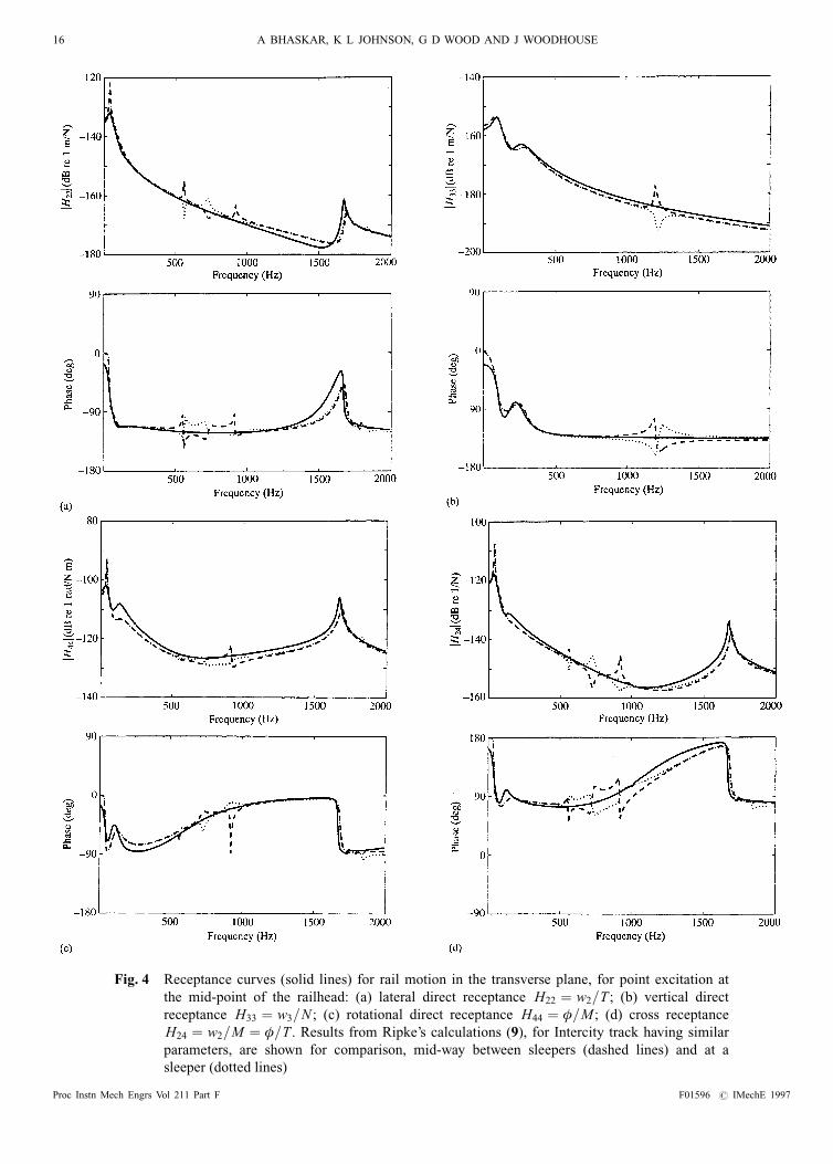
Fig. 4 Receptance curves (solid lines) for rail motion in the transverse plane, for point excitation at

the mid-point of the railhead: (a) lateral direct receptance H22 � w2=T ; (b) vertical direct

receptance H33 � w3=N ; (c) rotational direct receptance H44 � ö=M ; (d) cross receptance

H24 � w2=M � ö=T . Results from Ripke's calculations (9), for Intercity track having similar

parameters, are shown for comparison, mid-way between sleepers (dashed lines) and at a

sleeper (dotted lines)



which gives the linearized stiffness of the `Hertz spring' at

P � P0:

kH � dP

däz

� �0

� 6G2 P0 Re

(1ÿ í)2

" #1=3

(11)

The effect on steady state creepages of small changes in

force, Q9x, Q9y, P9, from a reference state Qx0, Qy0, P0, is

given by differentiation of equations (5a and b):

î9x

î9y

î9z

24 35 �@îx

@Qx

@îx

@Qy

@îx

@P

@î y

@Qx

@î y

@Qy

@î y

@P

0 0 0

266664377775

Q9x

Q9y

P9

24 35 (12)

where îx � îx0 � î9x and î y � î y0 � î9y. The vertical

`creepage' îz is also included for compatibility with later

matrix equations, but it is uninfluenced by the lateral

creepage and is determined only by the Hertz spring

stiffness, to be allowed for in the next subsection. The

matrix in equation (12) is denoted by B; expressions for the

derivatives are quoted in Appendix 1.

3.1.2 Transient creepage

With rapid changes in force, the creepage experiences a

transient delay in reaching the steady state. This effect has

been analysed in detail by Gross-Thebing (12). A simpli-

fied treatment of transient creepage in closed form is used

here, based on the notion of `tangential contact springs'

acting in series with the `creepage dashpots' which

represent the velocity-dependent behaviour of equation

(12). Details of the model are presented in Appendix 1.

It is required to calculate the response to small harmonic

variations in force Q9x, Q9y and P9 from a steady reference

state in which the steady creepages are îx0 and î y0 and the

forces are Qx0, Qy0 and P0. It is shown in Appendix 1 that

in response to harmonic variations in force of angular

frequency ù, there are harmonic variations in velocity v9x,v9y, v9z of the rail relative to the wheel at the point of

contact, given by

1

V

v9xv9yv9z

24 35 � iù

VA� B

� � Q9xQ9yP9

24 35 (13)

where V is the vehicle speed. The matrix A allows for the

elastic transient effects, as well as the vertical Hertz spring.

It can be written

A �a11 0 0

0 a22 0

0 0 a33

24 35 (14)

where the coefficients a11 and a22 are given in Appendix 1;

a33 is the compliance of the Hertz spring 1=kH, given by

equation (11). The matrix B is that of the derivatives of

steady creepage, expressed by equation (12).

3.2 High-spin model

Under conditions of close conformity the ellipse of contact

becomes long and thin (b� a), so that the theory under-

lying equation (5a and b) becomes a poor approximation

and a `strip theory' becomes more appropriate [see

reference (10), p. 268]. If the spin creep is high, as a result

of the large values of b, an approximation to the contact

mechanics can be obtained in closed form by neglecting

tangential compliance compared with the slip [see refer-

ence (10), p. 259]. In this simplification there is a point,

labelled C in Fig. 6, where, in the absence of lateral slip,

there would be no relative velocity between the surfaces.

This point C is known as the `spin pole'. Let it be a

distance sb from the centre of the contact O. The long-

itudinal creepage î 0x experienced by a strip at location y is

then given by

î 0x � îx ÿ yùz

V� îx ÿ ùzb

V

� �ç (15)

where ç � y=b and ùz is the angular velocity of spin. In

the wheel±rail contact of Fig. 5

Fig. 5 Wheel±rail contact geometry for a single contact

point: ë is the nominal conicity of the wheel



ùzb

V� b

R1

� �sin (ë� á)

at the spin pole î 0x � 0, so that s � (îxV=ùzb)

Now the longitudinal traction force per unit width acting

on the strip is

Q 0 � ìP 0 � 3ìP

4b

� �(1ÿ ç2) (16)

The traction force Qx1 acting to the right of the spin pole in

Fig. 6 is thus given by

Qx1 ��b

sb

Q 0 dy � 14ìP(2ÿ 3s� s3) (17a)

and that to the left of C by

Qx2 � ÿ� sb

ÿb

Q 0 dy � ÿ14ìP(2� 3sÿ s3) (17b)

whereupon

Qx � Qx1 � Qx2 � ÿ12ìP(3sÿ s3) (17c)

The spin moment M z is given by the sum of the moments

of Qx1 and Qx2 about O, i.e.

M z � M z1 � M z2

where the two components turn out to be equal

M z1 � ÿ 3ìPb

4

�1

s

(1ÿ ç2)ç dç

� M z2 � 3ìPb

4

� s

ÿ1

(1ÿ ç2)ç dç

� ÿ 3ìPb

16(1ÿ s2)2

(18)

It is now necessary to incorporate lateral creepage î y,

and its interaction with longitudinal and spin creepage.

This is done in Appendix 2, where the relationships

between the creep forces and moment and the creepages

are shown to be

Qx � ìP

4

(1ÿ s)

r1

(2ÿ 3s� s3)ÿ (1� s)

r2

(2� 3sÿ s3)

� �(19a)

Qy � ÿ ìP

4

t

r1

(2ÿ 3s� s3)� t

r2

(2� 3sÿ s3)

� �(19b)

and

M z �

ÿ 3ìPb

16

(1ÿ s)

r1

(2ÿ 3s� s3)� (1� s)

r2

(2� 3sÿ s3)

� �(19c)

in terms of dimensionless ratios t, r1 and r2 defined in

Appendix 2.

In this treatment, where the elastic strains are neglected

compared with the slip, the transient creep effect contained

in matrix A in Appendix 1 does not arise. The linear

contact mechanics model for harmonically oscillating

creepage then becomes

Q9x

Q9y

P9

2666437775 �

S11 S12 S13

S21 S22 S23

0 0 S33

2666437775

î9x

î9y

î9z

2666437775

� îs cot (ë� á)

b1

b2

0

2666437775è � S

î9x

î9y

î9z

2666437775� sè

(20)

where Sij are the derivatives of equations (19a) and (19b)

with respect to îx, î y and îz after P has been expressed in

terms of î9z via the Hertz spring relation

S33 � ÿ VkH

iù(21)

Fig. 6 Strip theory analysis used to obtain the high-spin

contact model for the case of close conformity

(b� a)



where kH is given by equation (11). The second term in

equation (20) involves the quantities b1 � @Qx=@îs,

b2 � @Qy=@îs and è(� á9), which is the angle subtended

by the displacement of the contact point from its reference

position.

The fluctuations in spin moment are found from

M9z � [ p1 p2 p3]

î9xî9yî9z

24 35 (22)

where pi are the derivatives of equation (19) with respect

to îx, î y and îz. The fluctuating power dissipation W 9,including the spin loss, is given by

W 9

V�ÿ Qx0î9x � Qy0î9y � M z0

R1

cos (ë� á)è

� Q9xîx0 � Q9yî y0 � M9zR1

sin (ë� á)

(23)

The question arises: under what conditions is the high-

spin model appropriate? The relevant parameter is

[b sin (ë� á)=ìa]; the model becomes a reasonable ap-

proximation when the value of this parameter exceeds 1.0.

Clearly its value increases with conformity as the ratio b=a

for the contact ellipse increases. The reference conditions

examined below and in the companion paper (1) corre-

spond to a value of approximately 1.5.

4 CONFORMAL CONTACT

4.1 Single moving point of contact

A significant feature of a closely conforming contact is that

small lateral and rotational displacements of the rail

relative to the wheel can cause a relatively large movement

of the contact point across the railhead. The geometry is

shown in Fig. 7. In the steady reference state the contact

point is located at A0. Oscillating rail displacements w2, w3

and ö are assumed to be excited by a ripple on the wheel or

rail surface which imposes a normal displacement Ä eiù t at

A0 and a rotation ø eiù t. The combination of the imposed

ripple and the rail motion causes an oscillatory lateral

motion rè of the point of contact where, in the context of a

linear theory, è must be assumed small. From the geometry

of Fig. 7, it follows that the shift of the point of contact

from A0 to A is given by

A0A � rè � K[rø� (w2 ÿ rö) cosá� w3 siná] (24)

so that è may be written in the form

è � K ø� ctw2

w3

ö

24 350@ 1A with

ct � (1=r)[cosá siná ÿ r cosá] (25)

The compression of the Hertz spring at A is given by

äz � Äÿ w3 cosá� (w2 ÿ rö) siná (26)

If the rolling radius at A0 is R1 and that at A is (R1 � R91)

R91 � r sin (ë� á)è

which introduces a fluctuating longitudinal velocity

v 0x � ÿ�rV

R1

�sin (ë� á)è (27)

The motion of the contact point is related to the displace-

ments of the wheel and rail by

Fig. 7 Geometry of a single moving point of contact

between closely conforming surfaces



v9x

v9y

v9z

2666437775�

ÿv 0x

0

iùÄ

2666437775 � iù

0 0 0

cosá siná 0

ÿsiná cosá r siná

2666437775

w2

w3

ö

2666437775

so that

1

V

v9xv9yv9z

24 35 � D

w2

w3

ö

24 35� jè� eÄ

with

j �ÿr sin (ë� á)=R1

0

0

24 35, e �0

0

ÿiù=V

24 35 (28)

The contact forces, Qx � Qx0 � Q9x etc. acting at A exert

tangential and normal forces (T0 � T 9) and (N0 � N 9)acting at O, together with a moment (M0 � M9), according

to

T 9

N 9

M9

2666437775 �

0 cosá ÿsiná

0 siná cosá

0 r(1ÿ cosá) r siná

2666437775

Q9x

Q9y

P9

2666437775

� è

ÿP0 cosáÿ Qy0 siná

ÿP0 siná� Qy0 cosá

P0 r cosá� Qy0 r siná

2666437775

(29)

i.e.

T 9N 9M9

24 35 � F

Q9xQ9yP9

24 35� èg (30)

The dynamic model of the rail may now be coupled to

one of the contact mechanics models described in the

previous section to obtain a complete model. For the case

of the high-spin model, the result is as shown in the block

diagram of Fig. 8. Static input comes in the form of the

steady reference state: îx0, î y0 and P0. Dynamic input is

provided by sinusoidal irregularities on the wheel or rail

surface in the form of a normal displacement Ä eiù t at A0

and a rotation ø eiù t about A0. The various vectors and

matrices S, s, c, D, e, F, g and j have all been defined in

the text, while the box labelled K denotes scalar multi-

plication by the conformity factor and HR is the matrix of

receptances from the rail model. A very similar diagram

can be constructed for the low-spin model, but it is not

reproduced here. It differs simply in that the box labelled s

is absent, and the matrix S from equation (20) must be

replaced by the matrix

iù

VA� B

� �ÿ1

from equation (13).

4.2 Two-point contact

If the situation occurs that the radius of curvature of the

wheel tread is locally less than that of the rail, two-point

contact will take place. This is an extreme case of

`conformal contact', and it is of some interest to analyse in

its own right. The detailed form of the wheel and rail

profiles determine the positions of the two contact points,

A and B, which will not change significantly in response to

motion of the rail (see Fig. 9). Since in this case there is no

lateral motion of the contact points, è � 0 in the equations

of the previous subsection. A complete model based on

two-point contact can be assembled on similar lines to that

for moving single-point contact. The input is now naturally

expressed as separate vertical `ripples' of displacement

ÄA eiù t at point A and ÄB eiù t at point B. The resultant

forces acting on the rail are obtained by adding the contact

forces arising at A and B

T 9N 9M9

24 35 � FA

Q9xQ9yP9

24 35A

�FB

Q9xQ9yP9

24 35B

(31)

where the matrices FA and FB are given by the expression

in equation (29), with á � áA and á � áB respectively.

Fig. 8 Block diagram for the complete (linearized) sys-

tem combining a single moving point of contact

(using the high-spin model) with the dynamic

response of the rail. Input is provided by the

assumed ripple characterized by Ä and ø, and

various output quantities are shown at the appro-

priate points on the network. Positive signs are

assumed at all summing junctions



Since the ellipticity of each contact patch is relatively

small, the low-spin contact model is appropriate in this

case. The resulting block diagram for the complete two-

point contact model is shown in Fig. 10.

5 STABILITY

The next step is to investigate whether the complete closed-

loop models described in the previous section exhibit linear

instability. If instability were found, it could be hypothe-

sized that small-amplitude oscillators might in fact grow

until roll±slip oscillation was occurring. To investigate

further would then require a non-linear treatment of the

problem, probably via numerical time-marching simula-

tion.

The somewhat complex interconnected loops of Fig. 8

require rather careful stability analysis. The approach is to

decompose the system into smaller units, each having the

form of the simple two-block feedback system of Fig. 11.

For any such system, standard control theory gives a

criterion for stability. The requirement is that for any input

signals w1(t) and w2(t) with finite energy (in other words,

a finite value of the integrated square of the functions over

all time), the internal signals e1(t) and e2(t) must have

finite energy and satisfy the condition of causality. This

requirement can be tested using the extended Nyquist

theorem (13): in terms of the Laplace transfer function

matrices H1(s) and H2(s) the system of Fig. 11 is internally

stable if and only if

(a) det (IÿH1(1)H2(1)) 6� 0;

(b) the number of right half-plane poles of the product

H1(iù)H2(iù) is equal to n1 � n2, where n1 and n2

are respectively the number of right half-plane poles

(counting multiplicities) of H1 and H2; and

(c) det (IÿH1(s)H2(s)) is non-zero and encircles the

origin n1 � n2 times as s traverses a contour which

passes down the imaginary axis from infinity, inden-

ting to the left of any imaginary axis poles, then

closes around an arbitrarily large semicircle in the

right half-plane.

The particular aim here is to investigate the influence on

stability of the conformity factor K. To this end, it is useful

to consider first the system with K � 0. This leaves the

loop shown in Fig. 12a, which has the form of Fig. 11. If

this subsystem can be shown to be stable, then it remains to

investigate whether the whole system can be destabilized

by introducing a non-zero value of K. For this, the

Fig. 9 Geometry of two-point contact, at the points A

and B

Fig. 10 Block diagram corresponding to Fig. 8, for the

complete system assuming two-point contact.

Positive signs are assumed at all summing junc-

tions

Fig. 11 Block diagram of canonical feedback network

Fig. 12a Block diagram of the system of Fig. 8 when

K � 0



contribution of K can be isolated in the form shown in Fig.

12b, where the box labelled H is simply the whole of the

rest of the system apart from the block K. In terms of the

matrices defined in the previous section, this transfer

function is found by straightforward algebraic manipulation

to be given by

H � ct(IÿHRFSD)ÿ1HR(g � Fs� FS j) (32)

Again, this system has the form of Fig. 11 so that the

Nyquist criterion can be applied directly.

To apply this stability test, the rail model and contact

model must be run with particular parameter values. The

values selected were those used in a survey of the forced

response behaviour of these models to be discussed in the

companion paper (1), and they are listed in Tables 1 and 2

of that reference. The Nyquist plot for the outer loop

representing the case K � 0 is shown in Fig. 13a. Figure

13b shows a close-up view of the region near the origin. It

is clear that there are no encirclements of the origin, and it

follows that the outer loop is internally stable. Two facts

must be noted in this connection. First, the rail model is a

passive mechanical system and cannot have any poles in

the closed right half-plane. Second, the system as it has

been formulated has an apparent pole-zero cancellation at

zero frequency (pole in S, zero in D). This arises from the

somewhat artificial introduction of the vertical `creepage'

v9z in place of the vertical displacement ä9z, and it can be

readily shown that it does not contribute to the pole count

needed for the Nyquist criterion.

A detail to be noted in these Nyquist plots and in the one

to follow is that the model has been slightly adjusted at

very low frequencies. The assumption of hysteretic damp-

ing in the rail pads and ballast produces non-physical

results at these low frequencies, manifesting itself in

Nyquist loops which do not close. To cure this in a way

which is simple but physically sensible, the imaginary parts

of the rail receptances at very low frequencies have been

forced to tend to zero, producing artificial kinks in the

Nyquist plots but giving the correct topology for the

purpose of the Nyquist criterion.

The Nyquist plot for the conformity factor loop of Fig.

12b is shown in Fig. 13c, for the particular case having

K � 1. It shows no encirclements of the origin, and so the

introduction of the additional feedback loops via K does

not produce instability. Since changing the value of K

Fig. 12b Block diagram for investigation of the influence

of conformity factor on stability

Fig. 13a Nyquist plot for the system of Fig. 12a

Fig. 13b Expansion of (a) near the origin

Fig. 13c Nyquist plot for the system of Fig. 12b



simply amounts to a scaling of this plot relative to the point

(1,0), this remains true for all possible values of K. This

result has been confirmed by checking the Nyquist

criterion for the complete system at a range of values of K.

The corresponding stability analysis has also been

carried out using the low-spin contact model of Appendix

1. The Nyquist plots corresponding to those of Fig. 13 are

different in detail, but are qualitatively very similar to those

shown here for the high-spin model. Neither loop encircles

the origin.

The conclusion is that the single-point contact model is

stable, for all values of the conformity factor K, at least

when coupled to the continuously supported rail model

employed here, with parameter values appropriate to

British Rail track. The dominant physical reason for this

strong stability appears to be associated with the high level

of vibration damping provided by the infinite rail modelÐ

energy in oscillation at the contact region is simply lost by

radiation of bending and torsional waves along the rail.

This conclusion is in a sense disappointing, since it shows

that the model analysed here does not immediately lead to

an explanation of some of the findings on the Vancouver

Skytrain system (scratch marks, and a variation of corru-

gation wavelength with train speed suggesting roll±slip

oscillation). It remains possible that instability might arise

if further features of the physical system were included in

the model. Candidates might be wheel resonances, and

perhaps the constraining effect of adjacent wheels of the

vehicle, reflecting back some of the vibrational energy

radiated along the rail. These are matters for future

research.

6 CONCLUSIONS

A dynamic model of the wheel±rail system has been set up

on the basis of a rigid wheel and a continuously supported

rail. Receptance curves for excitation at the railhead by

vertical force, horizontal force or moment have been

calculated over the range 0±2 kHz. These show good

agreement with the model described by Ripke (9), except

in certain narrow frequency bands which are strongly

influenced by the presence of discrete supports.

Two contact mechanics models, which relate dynamic

creep forces to fluctuating creepages, have been proposed.

The first applies under conditions of low-spin creepage,

and includes the transient effect which leads to frequency

dependent creep coefficients. The second applies under the

conditions of high spin which arise with close conformity,

when the contact region becomes highly elliptical. Tangen-

tial elastic deformations, and hence transient effects, are

neglected in this model, but they are in any case expected

to be small under conditions of close conformity and high

spin.

The effect of close conformity has been modelled in two

separate ways. In the first, the wheel and rail are assumed

to touch at one point, giving rise to a highly elliptical

contact region and high spin. Dynamic torsion of the rail

causes the point of contact to move laterally across the

railhead. In the second model of conformity, two separate

points of contact are assumed. These are taken to be

circular and not to move laterally across the railhead. In

this case, spin is effectively taken into account by imposing

a difference in the steady longitudinal creepages at the two

points of contact.

The stability of motion under these models has been

investigated, using linear theory, and it has been found that

the system is stable within the expected range of para-

meters and conformity. This conclusion holds for both low-

spin and high-spin contact models. It remains to investigate

the forced response of the models to a pre-existing surface

ripple on the rail or wheel, to determine whether wear

processes might be expected to deepen or to erase the

ripple, and hence to lead to growth or decay of short-pitch

corrugations. This issue is discussed in Part 2 of this paper

(1).

ACKNOWLEDGEMENTS

The authors thank B. Ripke and S. MuÈller for help with,

and permission to reproduce, the comparisons with the

Berlin rail model (9). The work reported here was carried

out with the support of a grant from ERRI committee

D185.

REFERENCES

1 Bhaskar, A., Johnson, K. L. and Woodhouse, J. Wheel±rail

dynamics with closely conformal contact. Part 2: forced

response, results and conclusions. Proc. Instn Mech. Engrs,

Part F, 1997, 211 (F1), 27±40.

2 Grassie, S. L. and Kalousek, J. Rail corrugation: character-

istics, causes and treatments. Proc. Instn Mech. Engrs, 1993,

207 (F2), 57±68.

3 Hempelmann, K. and Knothe, K. An extended linear model

for the prediction of short wavelength corrugation. Wear,

1996, 191, 161±169.

4 Frederick, C. O. A rail corrugation theory. Proceedings of

the 2nd International Conference on Contact Mechanics of

Rail=Wheel Systems, University of Rhode Island, 1986,

pp. 181±211 (University of Waterloo Press).

5 Valdivia, A. The interaction between high-frequency wheel±

rail dynamics and irregular rail wear. VDI-Fortschrittsbericht,

Reihe 12, Nr.93, 1988, Dusseldorf.

6 Kalousek, J. and Johnson, K. L. An investigation of short

pitch wheel and rail corrugation on the Vancouver mass transit

system. Proc. Instn Mech. Engrs, Part F, 1992, 206 (F2),

127±135.

7 Grassie, S. L., Gregory, R. W. and Johnson, K. L. The

behaviour of railway wheelsets and track at high frequencies

of excitation. J. Mech. Engng Sci., 1982, 24, 103±111.

8 Thompson, D. J. Wheel±rail noise generation, Part III: rail

vibration. J. Sound Vibration, 1993, 161, 421±446.

9 Ripke, B. and Knothe, K. Die unendlich lange Schiene auf



diskreten Schwellen bei harmonischer Einzellastanregung,

VDI Fortschritte, Reihe 11, N.155, 1991, Dusseldorf.

10 Johnson, K. L. Contact Mechanics, 1985 (Cambridge

University Press).

11 Kalker, J. J. Three-dimensional Elastic Bodies in Rolling

Contact, 1990 (Kluwer, Dordrecht).

12 Gross-Thebing, A. Lineare Modellierung des instationaren

Rollcontakts von Rad und Schiene, VDI-Fortschritte, Reihe 12

Nr.199, 1993, Dusseldorf.

13 Desoer, C. A. and Vidyasagar, M. Feedback Systems: Input±

Output Properties, 1975 (Academic Press, New York).

14 Frederick, C. O. A rail corrugation theory which allows for

contact patch size. Proceedings of Symposium on Rail Corru-

gation Problems, Berlin, 1991 (ILR-Bericht 59).

15 Johnson, K. L. The effect of a tangential contact force on the

rolling motion of an elastic sphere on a plane. Trans. ASME, J.

Appl. Mechanics, 1958, 25, 339±346.

16 Mindlin, R. D. Compliance of elastic bodies in contact. Trans.

ASME, J. Appl. Mechanics, 1949, 16, 259±268.

17 Mindlin, R. D. and Deresiewicz, H. Elastic spheres in contact

under varying oblique forces. Trans. ASME, J. Appl. Mech-

anics, 1953, 20, 327±345.

APPENDIX 1

Low-spin contact model

The steady creep equations (5a and b) may be written

îx � k1 P1=3 Qx

Q

� �1ÿ 1ÿ Q

ìP

� �1=3" #

� k1 f x (33a)

î y � k2 P1=3 � k1 P1=3 Qy

Q

� �1ÿ 1ÿ Q

ìP

� �1=3" #

� k1 f y

(33b)

where

k1 � 3ì

C00

16

9(1ÿ í)2 R2e G

� �1=3

(34)

and

k2 � C23

C00

sin (ë� á)

R1

3(1ÿ í)Re

4G

� �1=3

(35)

Kalker's creep coefficients as a function of (a=b) may be

expressed approximately by

C00 � 1=2(C11 � C22) � ÿ 2:84� 1:20a

b

� �� (36)

and

C23 � 0:40� 1:05a

b

� �(37)

The effect of small changes in Qx, Qy and P from a

reference state Qx0, Qy0 and P0 is found by differentiation

of (33a and b)

@ f x

@Qx

� P1=3Q2y

Q31ÿ 1ÿ Q

ìP

� �1=3" #

� 1

3ìP2=3

Qx

Q

� �2

1ÿ Q

ìP

� �ÿ2=3

(38a)

@ f y

@Qy

� P1=3Q2x

Q31ÿ 1ÿ Q

ìP

� �1=3" #

� 1

3ìP2=3

Qy

Q

� �2

1ÿ Q

ìP

� �ÿ2=3

(38b)

@ f x

@Qy

� @ f y

@Qx

� 1

3ìP2=3

QxQy

Q21ÿ Q

ìP

� �1=3

ÿ P1=3QxQy

Q31ÿ 1ÿ Q

ìP

� �1=3" # (38c)

@ f x

@P� 1

3P2=3

Qx

Q1ÿ 1ÿ Q

ìP

� �ÿ2=3" #

(38d)

@ f y

@P� 1

3P2=3

Qy

Q1ÿ 1ÿ Q

ìP

� �ÿ2=3" #

(38e)

The matrix B is now defined by

B � k1

@ f x

@Qx

@ f x

@Qy

@ f x

@P

@ f y

@Qx

@ f y

@Qy

@ f y

@Pÿ k2

k1

Pÿ2=3

� �0 0 0

266664377775 (39)

An elastic rolling contact with creepage has a contact

area which is divided into a region of adhesion (`stick') and

one of slip. A complete solution to the problem of transient

creep requires tangential elastic displacements of the two

bodies at the interface to satisfy the appropriate conditions

of stick and slip throughout the contact area ((10), }8.1).

This was first achieved by Kalker (11) in line contact with

longitudinal creepage only. A numerical approach to a

complete solution with general creepage has been obtained

by Gross-Thebing (12). A simplified approach, using the

elastic foundation or `wire±brush' contact model, has been

employed by Frederick (14) in his corrugation theory. The

closed-form expressions for non-linear steady creepage

(33a and b) are based on the assumption that the stick area

is an ellipse, similar to the contact ellipse, and tangential to

it at the leading point (ÿa, 0). This early theory (15) was

found to have errors of up to 25 per cent in the linear creep

coefficients compared with Kalker's exact values (11).



However, a good fit with experiment is obtained if the

linear coefficients are replaced by Kalker's values, while

retaining the functional form of f x and f y.

The compliance of a stationary contact with an elliptical

stick area has been found by Mindlin (16), with the results

äx � C44

2Gc

3ìP

2

Qx

Q1ÿ 1ÿ Q

ìP

� �2=3" #

(40a)

ä y � C55

2Gc

3ìP

2

Qy

Q1ÿ 1ÿ Q

ìP

� �2=3" #

(40b)

where for Poisson's ratio í � 0:3

C44 � ÿ0:85p

(a=b)[1� 1:14 log10 (b=a)] (41a)

C55 � ÿ0:85p

(a=b)[1� 1:57 log10 (b=a)] (41b)

The effect of small changes in Q9x, Q9y, P9 from the

reference state Qx0, Qy0, P0 depends upon whether the

forces are increasing or decreasing [see Mindlin and

Deresiewicz (17)]. The relationship of equation (40) is

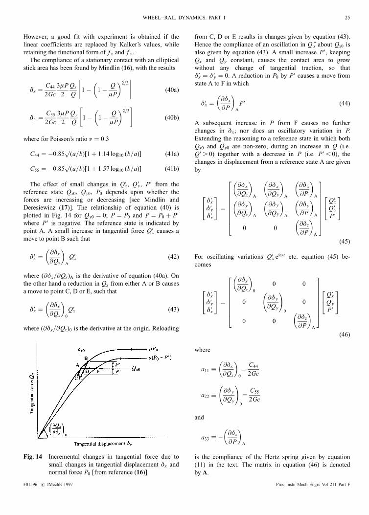
plotted in Fig. 14 for Qy0 � 0; P � P0 and P � P0 � P9where P9 is negative. The reference state is indicated by

point A. A small increase in tangential force Q9x causes a

move to point B such that

ä9x � @äx

@Qx

� �A

Q9x (42)

where (@äx=@Qx)A is the derivative of equation (40a). On

the other hand a reduction in Qx from either A or B causes

a move to point C, D or E, such that

ä9x � @äx

@Qx

� �0

Q9x (43)

where (@äx=@Qx)0 is the derivative at the origin. Reloading

from C, D or E results in changes given by equation (43).

Hence the compliance of an oscillation in Q 0x about Qx0 is

also given by equation (43). A small increase P9, keeping

Qx and Qy constant, causes the contact area to grow

without any change of tangential traction, so that

ä9x � ä9y � 0. A reduction in P0 by P9 causes a move from

state A to F in which

ä9x � @äx

@P

� �A

P9 (44)

A subsequent increase in P from F causes no further

changes in äx; nor does an oscillatory variation in P.

Extending the reasoning to a reference state in which both

Qx0 and Qy0 are non-zero, during an increase in Q (i.e.

Q9 . 0) together with a decrease in P (i.e. P9 , 0), the

changes in displacement from a reference state A are given

by

ä9xä9yä9z

24 35 �@ä x

@Qx

� �A

@ä x

@Q y

� �A

@ä x

@P

� �A

@ä y

@Qx

� �A

@ä y

@Q y

� �A

@ä y

@P

� �A

0 0@äz

@P

� �A

2666666664

3777777775Q9xQ9yP9

24 35

(45)

For oscillating variations Q9x eiù t etc. equation (45) be-

comes

ä9xä9yä9z

24 35 �@äx

@Qx

� �0

0 0

0@ä y

@Qy

!0

0

0 0@äz

@P

� �A

266666664

377777775Q9xQ9yP9

24 35

(46)

where

a11 � @äx

@Qx

� �0

� C44

2Gc

a22 � @ä y

@Qy

!0

� C55

2Gc

and

a33 � ÿ @äz

@P

� �A

is the compliance of the Hertz spring given by equation

(11) in the text. The matrix in equation (46) is denoted

by A.

Fig. 14 Incremental changes in tangential force due to

small changes in tangential displacement äx and

normal force P0 [from reference (16)]



Under conditions of varying creepage from a reference

state, it is now assumed that the instantaneous relative

velocity vector v9 between the two surfaces can be

expressed by the simple summation of the steady creepage

and the rate of change of the static compliance, i.e.

v9 � Vî9� dädt

(47)

where V is the vehicle speed. In terms of Q � [Qx, Qy, P]t,

equation (47) becomes

v9 � VBQ9� AdQ

dt(48)

For harmonic variations in Q9 of angular frequency ù

(1=V )v9 � [B� (iù=V )A]Q9 (49)

APPENDIX 2

High-spin contact model

In order to incorporate lateral creepage î y, and its inter-

action with longitudinal and spin creepage in a simple way,

choose a representative strip at a distance L from the spin

pole, where y � L locates the line of action of Qx1 when

s � 0, i.e. when îx � 0. Thus

L � M z1(0)=Qx1(0) � (3=16)ìPb=(1=2)ìP � (3=8)b

(50)

Now assume that L remains unchanged for all values of s,

so that

î 0x1 � ÿùzb

V

3

8(1ÿ s) � ÿîs(1ÿ s) (51a)

and

î 0x2 � �ùzb

V

3

8(1� s) � �îs(1� s) (51b)

where

îs � 3

8

ùzb

V

is the representative creepage due to spin. Now take

Qy1

Qx1

� î y

î 0x1

andQy2

Qx2

� î y

î 0x2

Writing

î1 � (î 0x21 � î2

y)1=2 (52a)

and

î2 � (î 0x22 � î2

y)1=2 (52b)

r1 � î1

îs

� [(1ÿ s)2 � t2]1=2

and

r2 � î2

îs

� [(1� s)2 � t2]1=2

where t � î y=îs.

Making use of equation (17a and b) from the text, for

which î y � 0, the following are obtained

Qx1 � ìP

4

(1ÿ s)

r1

(2ÿ 3s� s3) (53a)

and

Qx2 � ÿ ìP

4

(1� s)

r1

(2� 3sÿ s3) (53b)

Qy1 � ÿ ìP

4

t

r1

(2ÿ 3s� s3) (54a)

and

Qy2 � ÿ ìP

4

t

r2

(2� 3sÿ s3) (54b)

M z1 � ÿ 3ìP

16

(1ÿ s)

r1

(2ÿ 3s� s3) (55a)

and

M z2 � ÿ 3ìP

16

(1� s)

r2

(2� 3sÿ s3) (55b)



Wheel–rail dynamics with closely conformal contact …jw12/JW PDFs/Rails1.pdf · Wheel–rail...

Documents

Transcript of Wheel–rail dynamics with closely conformal contact …jw12/JW PDFs/Rails1.pdf · Wheel–rail...