What you still might want to know about microarrays

Brixen, 24 June 2013Wolfgang Huber

EMBL

Late 1980s: Lennon, Lehrach: cDNAs spotted on nylon membranes

1990s: Affymetrix adapts microchip production technology for in situ oligonucleotide synthesis (commercial, patent-fenced)

1990s: Brown lab in Stanford develops two-colour spotted array technology (open and free)

1998: Yeast cell cycle expression profiling on spotted arrays (Spellmann) and Affymetrix (Cho)

1999: Tumor type discrimination based on mRNA profiles (Golub)

2000-ca. 2004: Affymetrix dominates the microarray market

Since ~2003: Nimblegen, Illumina, Agilent (and others)

Throughout 2000‘s: CGH, CNVs, SNPs, ChIP, tiling arrays

Since ~2007: 2nd-generation sequencing (454, Solexa)

Brief history

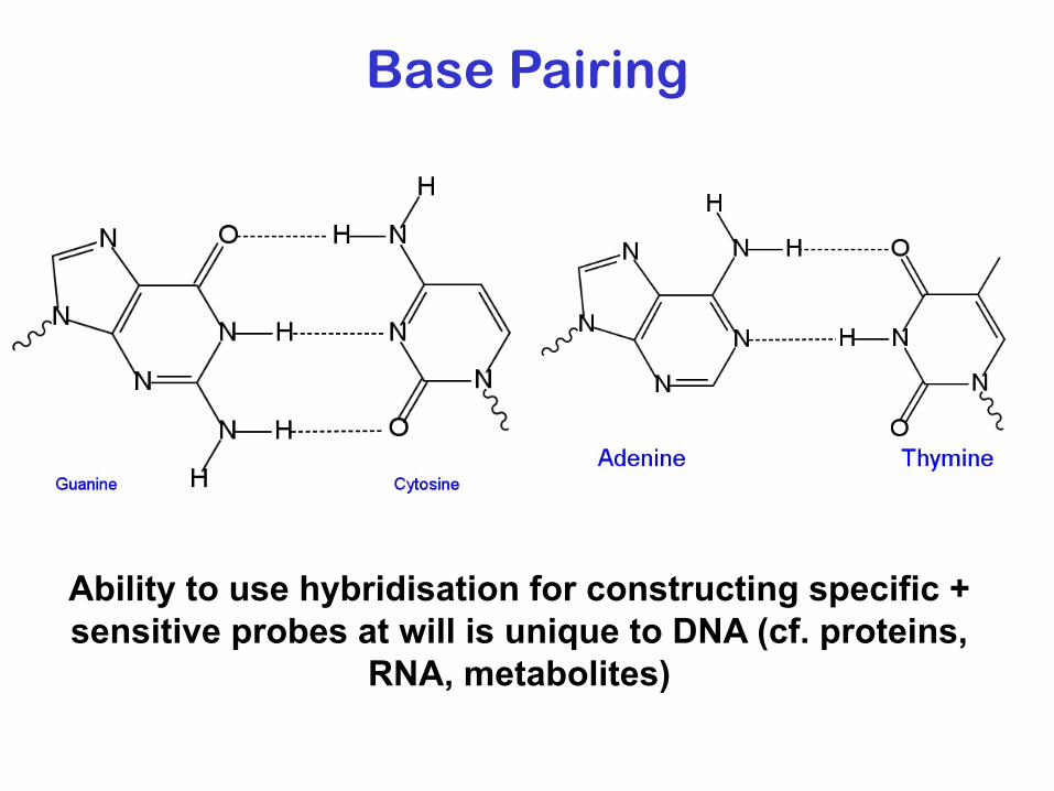
Base Pairing

Ability to use hybridisation for constructing specific + sensitive probes at will is unique to DNA (cf. proteins,

RNA, metabolites)

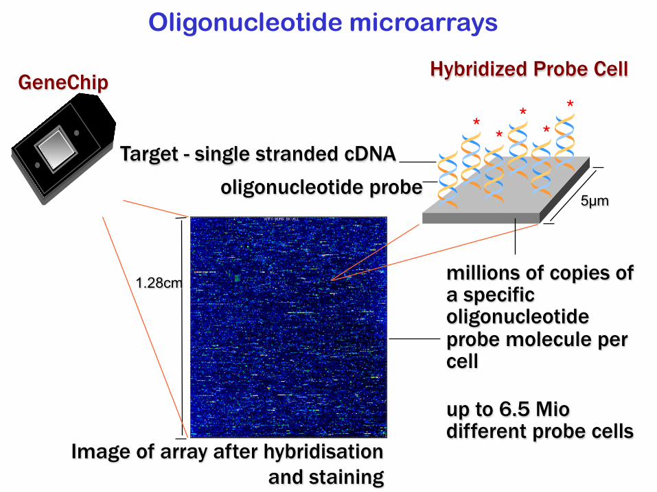
Oligonucleotide microarrays

5µm

millions of copies of a specific oligonucleotide probe molecule per cell

Image of array after hybridisation and staining

up to 6.5 Miodifferent probe cells

Target - single stranded cDNAoligonucleotide probe

* ****

1.28cm

GeneChip Hybridized Probe Cell

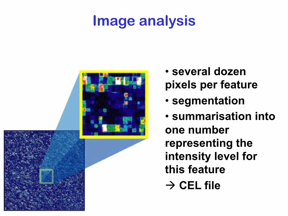
Image analysis

• several dozen pixels per feature• segmentation• summarisation into one number representing the intensity level for this feature à CEL file

µarray data

samples:mRNA fromtissue biopsies,cell lines

arrays:probes = gene-specific DNA strands

2.93

1.67

0.72

0.6

5.8

1.12

tissue B

3.314.2MCAM

0.671.32LAMA4

0.120.01CASP4

1.02.2ALDH4

1.81.1VIM

2.120.02ErbB2

tissue Ctissue A

fluorescent detection of the amount of

sample-probe binding

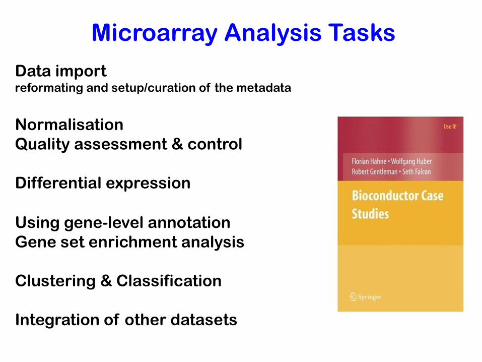
Microarray Analysis Tasks

Data importreformating and setup/curation of the metadata

NormalisationQuality assessment & control

Differential expression

Using gene-level annotationGene set enrichment analysis

Clustering & Classification

Integration of other datasets

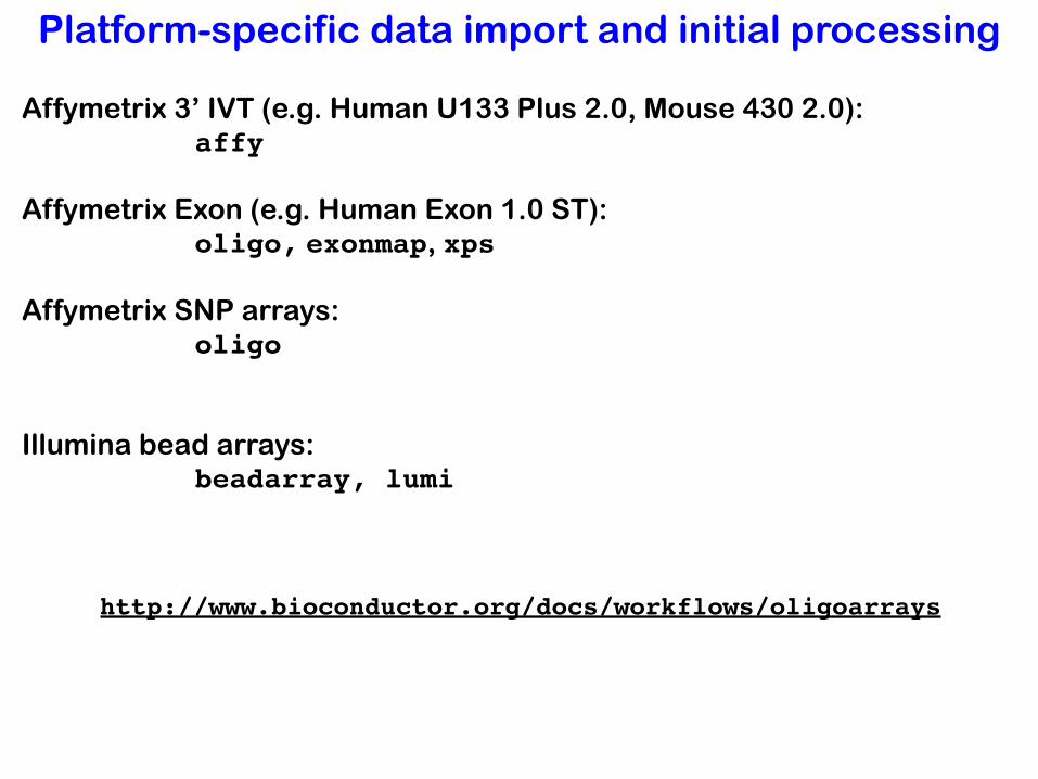
Platform-specific data import and initial processing

Affymetrix 3’ IVT (e.g. Human U133 Plus 2.0, Mouse 430 2.0): affy

Affymetrix Exon (e.g. Human Exon 1.0 ST): oligo, exonmap, xps

Affymetrix SNP arrays: oligo

Illumina bead arrays: beadarray, lumi

http://www.bioconductor.org/docs/workflows/oligoarrays

Flexible data import

Using generic R I/O functions and constructorsBiobaselimma

Chapter Two Color Arrays in the useR-book.limma user guide

Normalisation and quality assessment

preprocessCorelimmavsn

arrayQualityMetrics

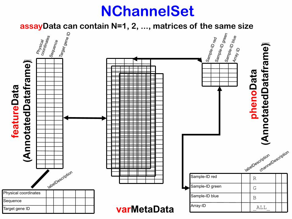
NChannelSetassayData can contain N=1, 2, ..., matrices of the same size

feat

ureD

ata

(Ann

otat

edD

ataf

ram

e)‏

D

Target gene ID

Sequence

Physical coordinates

Phys

ical

coor

dina

tes

Sequ

ence

Targ

et g

ene

ID

phen

oDat

a (A

nnot

ated

Dat

afra

me)‏

Sam

ple-

ID re

dSa

mpl

e-ID

gre

en

Arra

y ID

BSample-ID blue

_ALL_

G

R

Array-ID

Sample-ID green

Sample-ID red

Sam

ple-

ID b

lue

varMetaData

labelDescription labelDescr

iption

channelDescription

Annotation / Metadata

Keeping data together with the metadata (about reporters, target genes, samples, experimental conditions, ...) is one of the major principles of Bioconductor

• avoid alignment bugs

• facilitate discovery

→ Matrices with “rich” column and row names.

Annotation infrastructure for Affymetrix

hgu133plus2probe nucleotide sequence of the features (for preprocessing e.g. gcrma; for own annotation)hgu133plus2cdf maps the physical features on the array to probe setshgu133plus2.db maps probe sets to target genes and provides target gene annotation collected from public databases

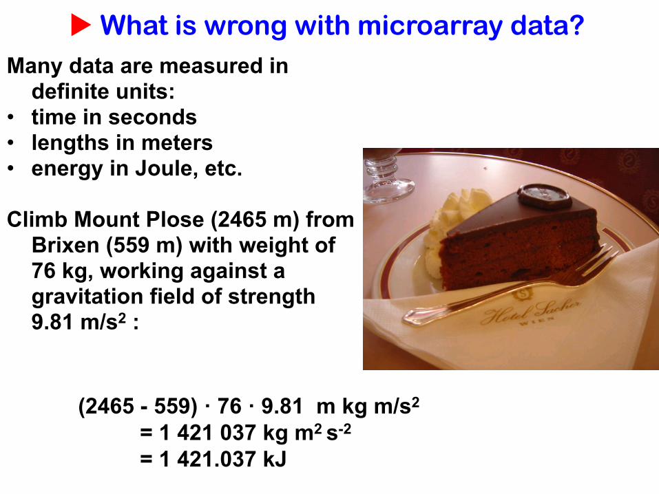
Many data are measured in definite units:

• time in seconds• lengths in meters• energy in Joule, etc. Climb Mount Plose (2465 m) from

Brixen (559 m) with weight of 76 kg, working against a gravitation field of strength 9.81 m/s2 :

u What is wrong with microarray data?

(2465 - 559) · 76 · 9.81 m kg m/s2

= 1 421 037 kg m2 s-2

= 1 421.037 kJ

A complex measurement process lies between mRNA concentrations and intensities

o RNA degradation

o quality of actual probe sequences (vs intended)

o image segmentation

o amplification efficiency

o scratches and spatial gradients on the array

o signal quantification

o reverse transcription efficiency

o cross-talk across features

o signal "preprocessing"

o hybridization efficiency and specificity

o cross-hybridisation

o labeling efficiency

o optical noise

The problem is less that these steps are ‘not perfect’; it is that they vary from array to array, experiment to experiment.

Background signal and non-linearities

log2Cope et al. Bioinformatics 2003

spike-in data“mild” non-linearity

linear range: y ~ x

saturation kicks in

background signal

u ratio compression

Yue et al., (Incyte

Genomics) NAR (2001)

29 e41

nominal 3:1

nominal 1:1

nominal 1:3

Statistical issues

tumor-normal

u Which genes are differentially transcribed?

same-same

log-ratio

u Sources of variationamount of RNA in the biopsy efficiencies of-RNA extraction-reverse transcription -labeling-fluorescent detection

probe purity and length distributionspotting efficiency, spot sizecross-/unspecific hybridizationstray signal

Calibration Error model

Systematic o similar effect on many measurementso corrections can be estimated from data

Stochastico too random to be ex-plicitely accounted for o remain as “noise”

Why do you need ‘normalisation’

(a.k.a. calibration)?

From: lymphoma dataset

vsn package

Alizadeh et al., Nature 2000

Systematic effects

Quantile normalisation

Ben Bolstad 2001

Within each column (array), replace the intensity values by their rank

For each rank, compute the average of the intensities with that rank, across columns (arrays)

Replace the ranks by those averages

arrays (samples)

feat

ure

s (g

en

es)

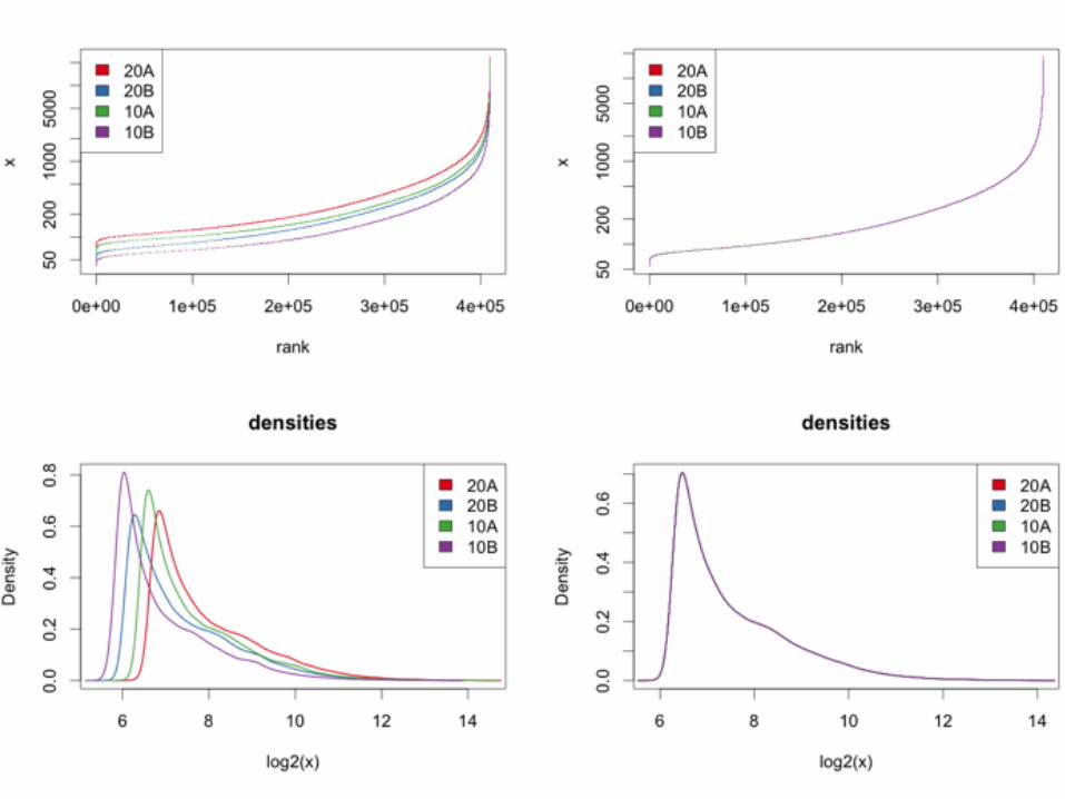
Quantile normalisation + Simple, fast, easy to implement+ Always works, needs no user interaction / tuning+ Non-parametric: can correct for quite nasty non-linearities

(saturation, background) in the data

- Always "works", even if data are bad / inappropriate- May be conservative: rank transformation looses

information - may yield less power to detect differentially expressed genes

- Aggressive: if there is an excess of up- (or down) regulated genes, it removes not just technical, but also biological variation

Less aggressive methods exist, e.g. loess, vsn

Estimating relative expression

(fold-changes)

u ratios and fold changesFold changes are useful to describe continuous changes in expression

10001500

3000x3

x1.5

A B C

0200

3000?

?

A B C

But what if the gene is “off” (below detection limit) in one condition?

u ratios and fold changesThe idea of the log-ratio (base 2) 0: no change +1: up by factor of 21 = 2 +2: up by factor of 22 = 4 -1: down by factor of 2-1 = 1/2 -2: down by factor of 2-2 = ¼

What about a change from 0 to 500?- conceptually- noise, measurement precision

A unit for measuring changes in expression: assumes that a change from 1000 to 2000 units has a similar biological meaning to one from 5000 to 10000.…. data reduction

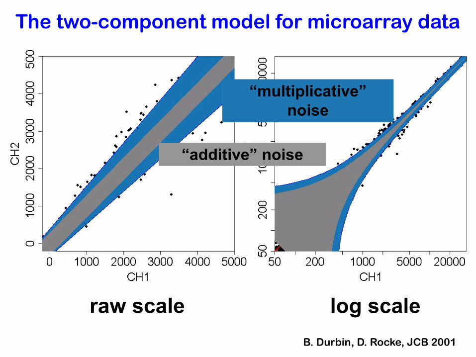
The two-component model for microarray data

raw scale log scale

“additive” noise

“multiplicative” noise

B. Durbin, D. Rocke, JCB 2001

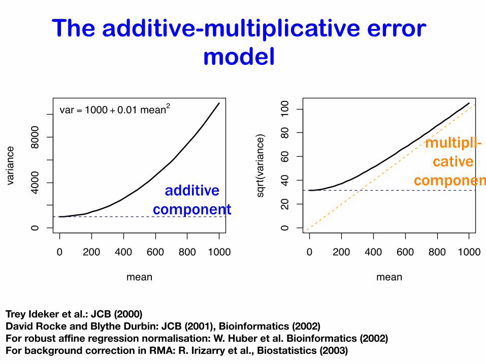
The additive-multiplicative error model

0 200 400 600 800 1000

04000

8000

mean

variance

var = 1000 + 0.01 mean2

0 200 400 600 800 1000

020

4060

80100

meansqrt(variance)

additive component

multipli-cative

component

Trey Ideker et al.: JCB (2000) David Rocke and Blythe Durbin: JCB (2001), Bioinformatics (2002) For robust affine regression normalisation: W. Huber et al. Bioinformatics (2002)For background correction in RMA: R. Irizarry et al., Biostatistics (2003)

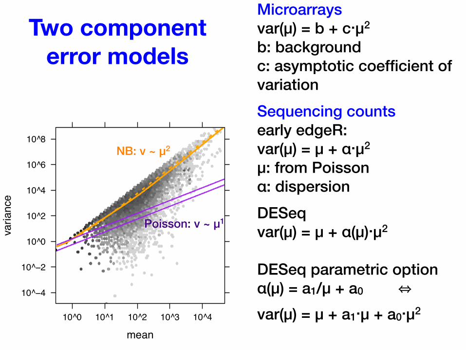
Two component error models

Microarraysvar(μ) = b + c⋅μ2

b: backgroundc: asymptotic coefficient of variationSequencing countsearly edgeR:var(μ) = μ + α⋅μ2

μ: from Poisson α: dispersionDESeqvar(μ) = μ + α(μ)⋅μ2

DESeq parametric optionα(μ) = a1/μ + a0 ⇔

var(μ) = μ + a1⋅μ + a0⋅μ2

mean

variance

10^−4

10^−2

10^0

10^2

10^4

10^6

10^8

10^0 10^1 10^2 10^3 10^4

Poisson: v ~ μ1

NB: v ~ μ2

u variance stabilizing transformation

f(x)

x

u variance stabilizing transformations

Xu a family of random variables with E(Xu) = u and Var(Xu) = v(u). Define

Then, var f(Xu ) ≈ does not depend on u

Derivation: linear approximation, relies on smoothness of v(u).

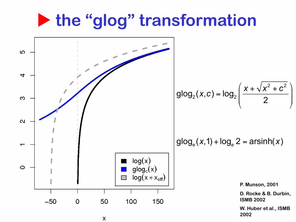
u the “glog” transformation

P. Munson, 2001

D. Rocke & B. Durbin, ISMB 2002

W. Huber et al., ISMB 2002

raw scale log glog

difference

log-ratio

generalized

log-ratio

constant partvariance:

proportional part

u glog

“usual” log-ratio

'glog' (generalized log-ratio)

c1, c2 are experiment specific parameters (~level of background noise)

u Variance-bias trade-off and shrinkage estimators

Same-same comparison

log-ratio

glog-ratio

Lines: 29 data points with observed ratio of 2

Fig. 5.11 from Hahne et al. (useR book)

u Variance-bias trade-off and shrinkage estimators

Shrinkage estimators:a general technology in statistics:pay a small price in bias for a large decrease of variance, so overall the mean-squared-error (MSE) is reduced.

Particularly useful if you have few replicates.

Generalized log-ratio is a shrinkage estimator for log fold change

Quality assessment

arrayQualityMetrics example quality report

u References

Bioinformatics and computational biology solutions using R and Bioconductor, R. Gentleman, V. Carey, W. Huber, R. Irizarry, S. Dudoit, Springer (2005).

Variance stabilization applied to microarray data calibration and to the quantification of differential expression. W. Huber, A. von Heydebreck, H. Sültmann, A. Poustka, M. Vingron. Bioinformatics 18 suppl. 1 (2002), S96-S104.

Exploration, Normalization, and Summaries of High Density Oligonucleotide Array Probe Level Data. R. Irizarry, B. Hobbs, F. Collins, …, T. Speed. Biostatistics 4 (2003) 249-264.

Error models for microarray intensities. W. Huber, A. von Heydebreck, and M. Vingron. Encyclopedia of Genomics, Proteomics and Bioinformatics. John Wiley & sons (2005).

Normalization and analysis of DNA microarray data by self-consistency and local regression. T.B. Kepler, L. Crosby, K. Morgan. Genome Biology. 3(7):research0037 (2002)

Statistical methods for identifying differentially expressed genes in replicated cDNA microarray experiments. S. Dudoit, Y.H. Yang, M. J. Callow, T. P. Speed. Technical report # 578, August 2000 (UC Berkeley Dep. Statistics)

A Benchmark for Affymetrix GeneChip Expression Measures. L.M. Cope, R.A. Irizarry, H. A. Jaffee, Z. Wu, T.P. Speed. Bioinformatics (2003).

....many, many more...

Acknowledgements

Anja von Heydebreck (Merck, Darmstadt)Robert Gentleman (Genentech, San Francisco)Günther Sawitzki (Uni Heidelberg)Martin Vingron (MPI, Berlin)Rafael Irizarry (JHU, Baltimore)Terry Speed (UC Berkeley)Lars Steinmetz (EMBL Heidelberg)Audrey Kauffmann (Novartis, Basel)David Rocke (UC Davis)

Summaries for Affymetrix genechip probe sets

Data and notationPMikg , MMikg = Intensities for perfect match and mismatch probe k for gene g on chip i i = 1,…, n one to hundreds of chipsk = 1,…, J usually 11 probe pairsg = 1,…, G tens of thousands of probe sets.

Tasks: calibrate (normalize) the measurements from different chips

(samples)summarize for each probe set the probe level data, i.e., 11 PM

and MM pairs, into a single expression measure.compare between chips (samples) for detecting differential

expression.

Expression measures: MAS 4.0

Affymetrix GeneChip MAS 4.0 software used AvDiff, a trimmed mean:

o sort dk = PMk -MMk o exclude highest and lowest valueo K := those pairs within 3 standard deviations of

the average

Expression measures MAS 5.0

Instead of MM, use "repaired" version CT CT = MM if MM<PM = PM / "typical log-ratio" if MM>=PM

Signal = Weighted mean of the values log(PM-CT) weights follow Tukey Biweight function (location = data median, scale a fixed multiple of MAD)

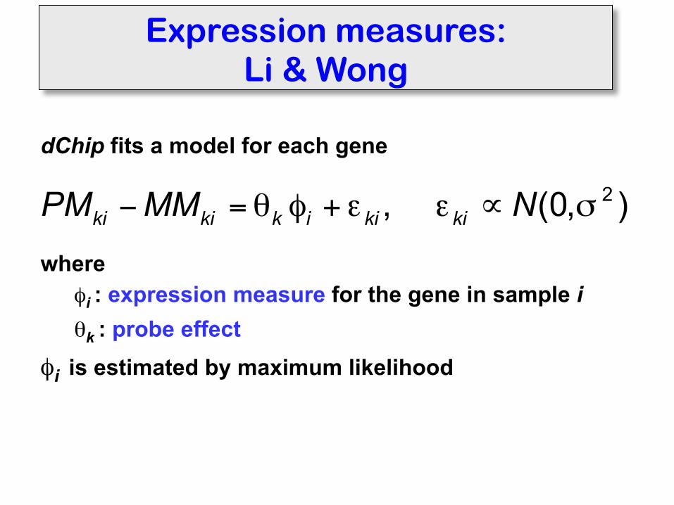
Expression measures: Li & Wong

dChip fits a model for each gene

whereφi : expression measure for the gene in sample iθk : probe effect

φi is estimated by maximum likelihood

dChip

RMA

bi is estimated using the robust method median polish (successively remove row and column medians, accumulate terms, until convergence).

Expression measures RMA: Irizarry et al. (2002)

further background

correction methods

Background correction

Irizarry et al. Biostatistics 2003

0 pm

500 fm 1 pm

750 fm

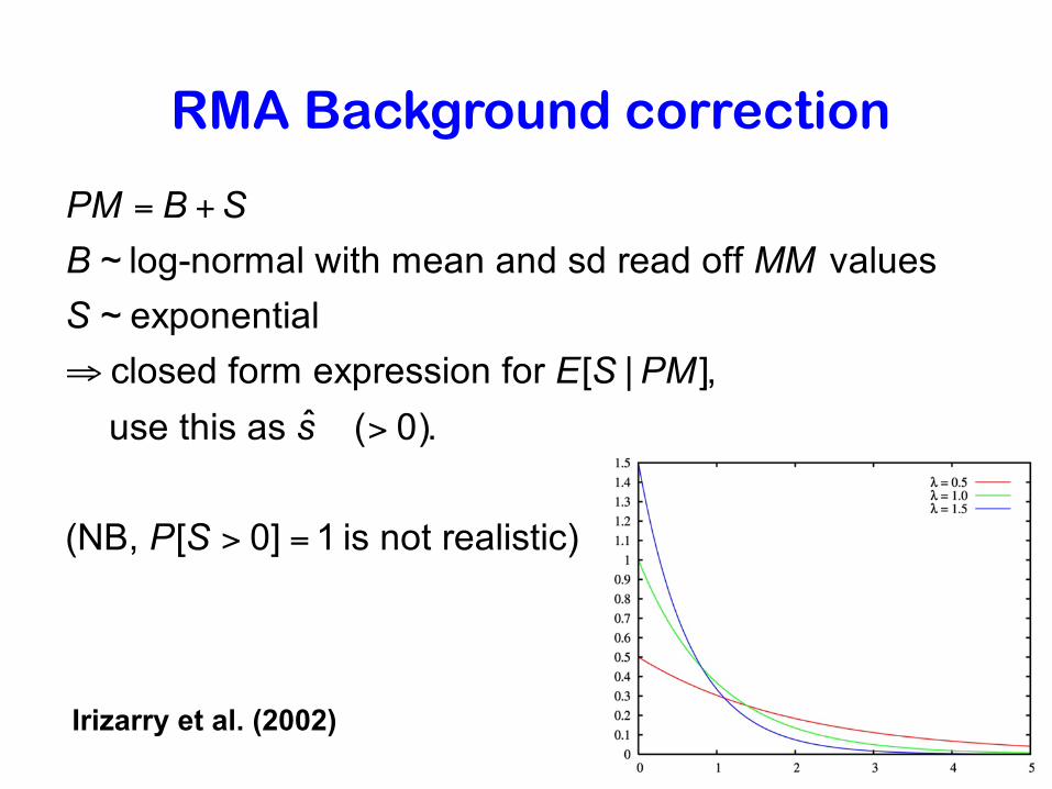
RMA Background correction

Irizarry et al. (2002)

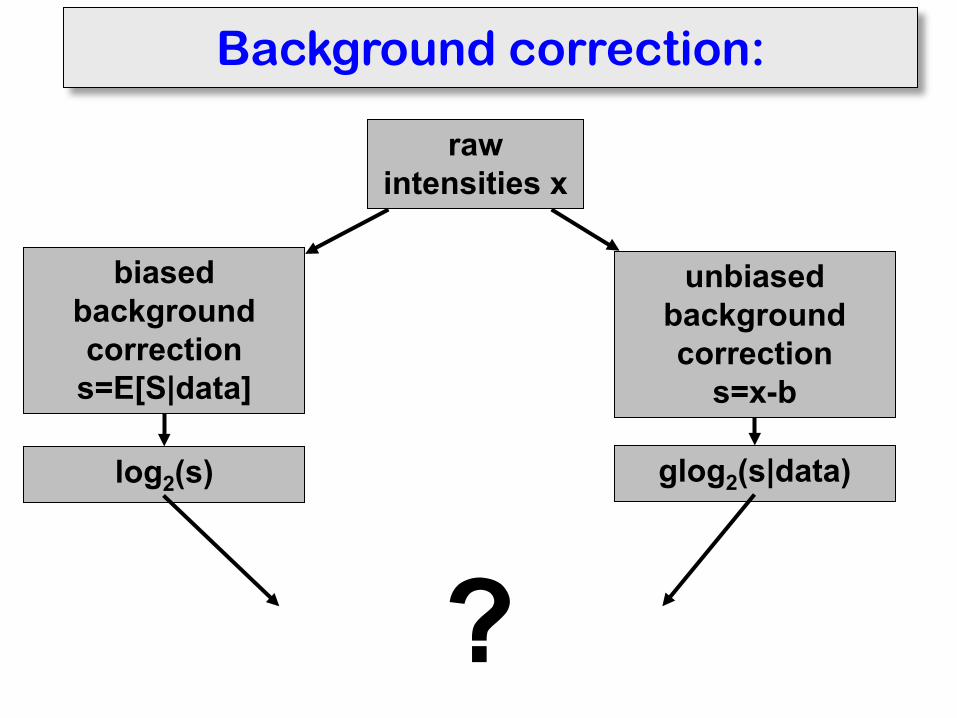
Background correction:

raw intensities x

biased background correction

s=E[S|data]

unbiased background correction

s=x-b

log2(s) glog2(s|data)

?

Comparison between RMA and VSN background correction

vsn package vignette

Figure 6: Results of vsnrma and rma on the Dilution example data. Array 1 was hybridised with 20µgRNA from liver, array 3 with 10µg of the same RNA.

method for NChannelSet. The return value is anNChannelSet, shown in Table 2. Note that, due tothe flexibility in the amount and quality of meta-data that is in an RGList, and due to di�erencesin the implementation of these classes, the transferof the metadata into the NChannelSet may not al-ways produce the expected results, and that somechecking and often further dataset-specific postpro-cessing of the sample metadata and the array fea-ture annotation is needed. For the current exam-ple, we construct the AnnotatedDataFrame objectadf and assign it into the phenoData slot of lym-NCS.

> vmd = data.frame(

+ labelDescription=I(c("array ID",

+ "sample in G", "sample in R")),

+ channel=c("_ALL", "G", "R"),

+ row.names=c("arrayID", "sampG", "sampR"))

> arrayID = lymphoma$name[wr]

> stopifnot(identical(arrayID,

+ lymphoma$name[wg]))

> ## remove sample number suffix

> sampleType = factor(sub("-.*", "",

+ lymphoma$sample))

> v = data.frame(

+ arrayID = arrayID,

+ sampG = sampleType[wg],

+ sampR = sampleType[wr])

> v

arrayID sampG sampR1 lc7b047 reference CLL2 lc7b048 reference CLL3 lc7b069 reference CLL4 lc7b070 reference CLL5 lc7b019 reference DLCL6 lc7b056 reference DLCL7 lc7b057 reference DLCL8 lc7b058 reference DLCL

> adf = new("AnnotatedDataFrame",

+ data=v,

+ varMetadata=vmd)

> phenoData(lymNCS) = adf

Now let us combine the red and green values fromeach array into the glog-ratio M and use the linearmodeling tools from limma to find di�erentially ex-pressed genes (note that it is often suboptimal toonly consider M, and that taking into account ab-solute intensities as well can improve analyses).

> lymM = (assayData(lymNCS)$R -

+ assayData(lymNCS)$G)

> design = model.matrix( ~ lymNCS$sampR)

> lf = lmFit(lymM, design[, 2, drop=FALSE])

> lf = eBayes(lf)

Figure 7 on page 7 shows the resulting p-values andthe expression profiles of the genes correspondingto the top 5 features.

6