WHAT IS DIFFERENT ABOUT URBANIZATION IN RICH … · What is Different About Urbanization in Rich...
62
NBER WORKING PAPER SERIES WHAT IS DIFFERENT ABOUT URBANIZATION IN RICH AND POOR COUNTRIES? CITIES IN BRAZIL, CHINA, INDIA AND THE UNITED STATES Juan Pablo Chauvin Edward Glaeser Yueran Ma Kristina Tobio Working Paper 22002 http://www.nber.org/papers/w22002 NATIONAL BUREAU OF ECONOMIC RESEARCH 1050 Massachusetts Avenue Cambridge, MA 02138 February 2016 We acknowledge support from the Taubman Center for State and Local Government. Chauvin acknowledges support from the Center for International Development at Harvard University. The views expressed herein are those of the authors and do not necessarily reflect the views of the National Bureau of Economic Research. At least one co-author has disclosed a financial relationship of potential relevance for this research. Further information is available online at http://www.nber.org/papers/w22002.ack NBER working papers are circulated for discussion and comment purposes. They have not been peer- reviewed or been subject to the review by the NBER Board of Directors that accompanies official NBER publications. © 2016 by Juan Pablo Chauvin, Edward Glaeser, Yueran Ma, and Kristina Tobio. All rights reserved. Short sections of text, not to exceed two paragraphs, may be quoted without explicit permission provided that full credit, including © notice, is given to the source.
Transcript of WHAT IS DIFFERENT ABOUT URBANIZATION IN RICH … · What is Different About Urbanization in Rich...
NBER WORKING PAPER SERIES
WHAT IS DIFFERENT ABOUT URBANIZATION IN RICH AND POOR COUNTRIES?CITIES IN BRAZIL, CHINA, INDIA AND THE UNITED STATES
Juan Pablo ChauvinEdward Glaeser
Yueran MaKristina Tobio
Working Paper 22002http://www.nber.org/papers/w22002
NATIONAL BUREAU OF ECONOMIC RESEARCH1050 Massachusetts Avenue
Cambridge, MA 02138February 2016
We acknowledge support from the Taubman Center for State and Local Government. Chauvinacknowledges support from the Center for International Development at Harvard University. Theviews expressed herein are those of the authors and do not necessarily reflect the views of theNational Bureau of Economic Research.
At least one co-author has disclosed a financial relationship of potential relevance for this research.Further information is available online at http://www.nber.org/papers/w22002.ack
NBER working papers are circulated for discussion and comment purposes. They have not been peer-reviewed or been subject to the review by the NBER Board of Directors that accompanies officialNBER publications.
© 2016 by Juan Pablo Chauvin, Edward Glaeser, Yueran Ma, and Kristina Tobio. All rights reserved.Short sections of text, not to exceed two paragraphs, may be quoted without explicit permission providedthat full credit, including © notice, is given to the source.
What is Different About Urbanization in Rich and Poor Countries? Cities in Brazil, China,India and the United StatesJuan Pablo Chauvin, Edward Glaeser, Yueran Ma, and Kristina TobioNBER Working Paper No. 22002February 2016JEL No. O15,O18,R12,R23
ABSTRACT
Are the well-known facts about urbanization in the United States also true for the developing world?We compare American metropolitan areas with comparable geographic units in Brazil, China andIndia. Both Gibrat’s Law and Zipf’s Law seem to hold as well in Brazil as in the U.S., but China andIndia look quite different. In Brazil and China, the implications of the spatial equilibrium hypothesis,the central organizing idea of urban economics, are not rejected. The India data, however, repeatedlyrejects tests inspired by the spatial equilibrium assumption. One hypothesis is that the spatial equilibriumonly emerges with economic development, as markets replace social relationships and as human capitalspreads more widely. In all four countries there is strong evidence of agglomeration economies andhuman capital externalities. The correlation between density and earnings is stronger in both Chinaand India than in the U.S., strongest in China. In India the gap between urban and rural wages is huge,but the correlation between city size and earnings is modest. The cross-sectional relationship betweenarea-level skills and both earnings and area-level growth are also stronger in the developing worldthan in the U.S. The forces that drive urban success seem similar in the rich and poor world, even iflimited migration and difficult housing markets make it harder for a spatial equilibrium to develop.
Juan Pablo ChauvinJFK School of Government79 JFK StreetCambridge, MA [email protected]
Edward GlaeserDepartment of Economics315A Littauer CenterHarvard UniversityCambridge, MA 02138and [email protected]
Yueran MaHarvard [email protected]
Kristina TobioKennedy School of Government79 JFK St- T347Cambridge, MA [email protected]
I. Introduction
The majority of the world’s urban population will soon live in places that are far poorer than the U.S. and
Europe. This creates a knowledge mismatch, for urban economists have predominantly focused on the cities
of the wealthy west. The relevance of the long literatures on wealthy world urbanization depends on the
similarity between poor world urbanization and rich world urbanization. This paper asks whether the major
stylized facts about the cities in the U.S. also hold for Brazil, China and India.
Economists frequently assume that our models work everywhere, although different levels of income and
education may create marginal differences. Yet the enormous social and political differences between the U.S.
and countries like Brazil, India and China may belie that assumption. For example, the central organizing
model of urban economics is the spatial equilibrium, which starts with the assumption of free mobility across
space. Does that assumption make sense in a country like China, which historically imposed legal barriers
to mobility such as the Hukuo system (Au and Henderson, 2006b)?
We focus on three major areas of research: core facts about city size, characterized by Zipf’s and Gibrat’s
Law, the Rosen (1979) and Roback (1982) spatial equilibrium, and the determinants of urban success,
including agglomeration economies, and human capital effects on wages and city growth. The transferability
of Zipf’s and Gibrat’s Law is of primarily academic interest. The transferability of the spatial equilibrium
framework determines our ability to rely on that framework’s many implications, such as the implication that
the benefits of new infrastructure for local renters will be muted by higher prices. Economists might want
to be far more circumspect about championing human capital and agglomeration if there is little evidence
that human capital externalities and agglomeration economies exist in the developing world.
Section II of this paper describes the data, which can be particularly problematic in the developing world.
For the U.S., we will work with Census-defined metropolitan areas using standardized geographic boundaries
based on the latest definitions. We tried to duplicate this structure for the other three countries, relying
whenever possible on standard Census-like products, but even the definition of metropolitan areas could be
difficult. In the case of India, for example, we use districts, but include only the urban population. Our time
frame runs from 1980 to 2010.
In Section III we present the basic facts about the distributions of populations across city sizes. While
Zipf’s Law is often considered to be a universal truth, like Soo (2014) we do not find it so. Standard
statistical tests reject the hypothesis that China, India and the U.S. are characterized by the same power
law distribution. Most notably, China and India have fewer extremely large sizes than would be predicted
by Zipf’s Law. Gibrat’s Law, which claims that growth rates are independent of initial population levels,
holds roughly for the U.S. and Brazil. It does not hold for India and China. In both of these countries,
urban population levels show substantial mean reversion from 1980 to 2010. Following the logic of Gabaix
(1999), the failure of Gibrat’s Law in these countries may explain why Zipf’s Law also fails to hold, perhaps
because India and China are still finding their way towards an urban steady state.
Section IV turns to the spatial equilibrium, which has long been the organizing principle of urban eco-
nomics. We do not focus on the intra-urban implications of the spatial equilibrium, developed by Alonso
2
(1964), but rather than inter-urban implications developed by Rosen (1979) and Roback (1982). Perhaps the
most basic implication of that model is that urban advantages in one area should be set off by countervailing
disadvantages in some other area. Higher wages should be offset by either lower amenities or higher housing
costs.
In the U.S., a one-log-point increase in area incomes (estimated as the residual from a regression where
earnings are regressed on human capital and demographics) is associated with a 1.6 log-points increase in
annual rents. This relationship is actually too small, relative to the predictions of the Rosen-Roback model,
unless higher income areas have low amenities or higher levels of unobserved human capital.
The comparable elasticities of area rents to area earnings for Brazil and China are 1.4 and 1.1 respectively.
As in the U.S., the earnings-rent relationships in these countries are quite strong, but smaller in magnitude
than theory would suggest. By contrast, the relationship between earnings and rents in India is practically
non-existent. This finding can imply either that Indian rental data is problematic, Indian rental markets
are dysfunctional, or that the spatial equilibrium does not hold in India. We suspect that the truth involves
some combination of all three explanations.
A second implication of the spatial equilibrium is that real wages should be lower in areas with better
natural amenities. Within the U.S., real wages rise, primarily because housing costs fall, in areas with less
temperate climate. In Brazil, real wages are higher in more temperate areas, primarily because nominal
wages are much lower in the hottest areas of the country. We suspect this reflects a combination of omitted
human capital and imperfect mobility. There is no relationship between climate and real wages in either
India or China, perhaps because these countries are not rich enough for ordinary workers to sacrifice earnings
for nicer weather.
We also look at income and self-reported happiness across space in the U.S., India and China (data is not
available for Brazil). Income and happiness are only weakly related across U.S. cities, which suggests that
higher incomes in U.S. metropolitan areas are not generating outsized improvements in personal welfare.
Across Chinese and Indian metropolitan areas, the income-happiness relationship appears stronger, even if it
is imprecisely measured. A stronger relationship could suggest that differences in unobserved human capital
are larger across cities in developing countries than in the U.S., or again, that the spatial equilibrium has
weaker predictive power in these countries.
The fundamental idea behind the spatial equilibrium is that migrants move to equalize welfare levels
across space, which seemed distinctly plausibly in the highly mobile U.S. Five-year mobility rates in China
and Brazil are lower than historic U.S. mobility rates, but the drop in U.S. mobility since 2000 and the
rise in Chinese mobility means that the three countries look broadly similar today. India, however, appears
to be far less mobile, which may explain why the Indian data does not seem well explained by the spatial
equilibrium model.
The case for spatial equilibrium is stronger in the U.S. than in the developing countries. Brazil and China
do have reasonably high migration rates and a strong correlation between income and housing costs. India
has low migration rates and essentially no correlation between income and rents. There is no compensation
for less temperate climates in any of the developing countries. We conclude from this subsection that the
3
spatial equilibrium framework can be used, if it is used warily, in Brazil and China. We see little reason for
confidence in the framework when applied to India.
Section V turns to the determinants of local success, such as agglomeration economies and human capital
spillovers. As is well known (e.g. Glaeser and Gottlieb, 2009), there are two standard problems with
agglomeration regressions: unobserved personal heterogeneity and unobserved place-based heterogeneity.
We address these issues in the limited ways that are standard in the literature (see Combes and Gobillon,
2014, for a discussion), controlling for observable human capital and instrumenting for current population
levels with population levels from 1980 and the start of the 20th century.
In the U.S., we estimate an agglomeration coefficient of .054 when the logarithm of male earnings is
regressed on metropolitan area population. The coefficient on the logarithm of density is slightly smaller
(.046). Our Brazilian estimates are similar to those in the U.S. The elasticity of wages with respect to area
population is .052 in Brazil, and the elasticity of wages with respect to area density is .026. In the U.S., we
estimate a “real wage” (defined as wages controlling for area rents) elasticity of approximately .02. In Brazil,
the elasticity is 0.01, which is not statistically significant.
By contrast, the estimated agglomeration effects are noticeably higher in both China and India, especially
with regard to area density. The density elasticity in China is .19. The population elasticity is half the
size, which is still higher than the estimated U.S. elasticity, but the Chinese coefficient is not statistically
significant. The Indian density elasticity is .076, which is similar to its population elasticity. In India there is
also a substantial real-wage premium associated with denser areas and larger urban populations, which again
suggests either the unobserved human capital differences are enormous or that India is not characterized by
a spatial equilibrium. In China, the real-wage elasticity to density (.052) is comparable to the one in India,
but the population elasticity is negative and statistically insignificant.
We then estimate human capital externalities by following Rauch (1993) and Moretti (2004) and re-
gressing the logarithm of earnings on area-level education (measured as the share of adults with tertiary
degrees), individual education and other demographic variables. We acknowledge the significant problem
that unobserved human capital may be correlated with measured area-level human capital, but we have no
way of solving that problem. Our estimated coefficient for the U.S. is 1.0, suggesting that a ten percent
increase in the share of adults with college degrees is associated with an approximately 10 percent increase
in earnings.
The comparable coefficients for Brazil, China and India are 4.7, 5.3 and 1.9 respectively. These results
suggest that an area-level increase in education in those countries is associated with a far higher increase in
the logarithm of earnings than in the U.S. The share of the population with a college degree varies far more
across U.S. cities than across developing world cities, so that the impact of a standard deviation increase in
area level education is more similar across the four countries.
Finally, we end with the correlation between human capital and the growth of urban populations and
income levels. In the U.S., a one percentage point increase in the share of adults with college degrees in
1980 is associated with a 2.2 percentage point increase in population growth between 1980 and 2010 and a .9
percentage point increase in income growth. These results have been taken as evidence for skills-enhancing
4
local productivity growth (Glaeser et al., 1995) or the increasing importance of human capital externalities
(Glaeser and Saiz, 2004).
The comparable effects in Brazil are far stronger. A one percentage point increase in the share of adults
with a college degree in Brazil is associated with an almost six percentage point increase in population growth
from 1980 to 2010 and a twelve percentage point increase in income growth. Again, the impact of skill seems
larger in the developing world, although the differences narrow if we consider the impact of a one standard
deviation increase in the skills measure.
The impact of skills on population growth in China is even larger. A one percentage point higher increase
share of adults with a college degree is associated with a 22 percentage point increase in population growth
from 1980 to 2010. The measured impact on income growth is negative and statistically insignificant. We do
not have results on income change in India, but education is a weaker predictor of population growth than
in the other developing-world countries. A one percentage point increase in the college educated share in
1980 is associated with only a .34 percentage point increase in population growth over the next thirty years,
and the estimate is not statistically significant.
Agglomeration economies and human capital externalities appear robust in the developing world. The
correlation between skills and urban growth is extremely strong in China and Brazil. Consequently, two major
policy lessons from U.S. data –skills matter for urban success and agglomeration increases productivity– seem
to be quite relevant for the developing world.
We conclude that there are both similarities and differences between urbanization in the U.S. and urban-
ization in the developing world. The core determinants of productivity –human capital and agglomeration–
are important everywhere. But anyone who assumes that India is in spatial equilibrium is making a leap of
faith.
One interpretation of these results is that the spatial equilibrium framework is not particularly relevant in
poor, traditional economies, where human-capital heterogeneity is enormous and people remain rooted to the
communities of their birth. Looking across the four countries, it seems quite possible that spatial equilibrium
emerges with development as human capital becomes more widespread and as people turn to markets instead
of traditional social arrangements in their home villages. The transition to a spatial equilibrium seems like
a fertile topic for future research.
II. Measuring Urban Areas in Four Countries
American urban research often examines variation across metropolitan areas. This research is possible
because the United States has a dispersed urban system with a large number of metropolitan areas that have
a rich variety of sizes, education levels and incomes. To examine the differences and similarities between the
developed and developing world, we chose three countries that are also large, populous and endowed with
a dispersed urban hierarchy: Brazil, China and India. These three countries are notable not only for their
size, but also for the fact that they are not dominated by a single urban giant, such as Buenos Aires, Jakarta
or Mexico City.
5
While these three countries are frequently linked together as BRICs, they have substantially different
income levels. Per capita GDP in India is approximately one-third of per capita income in Brazil, and
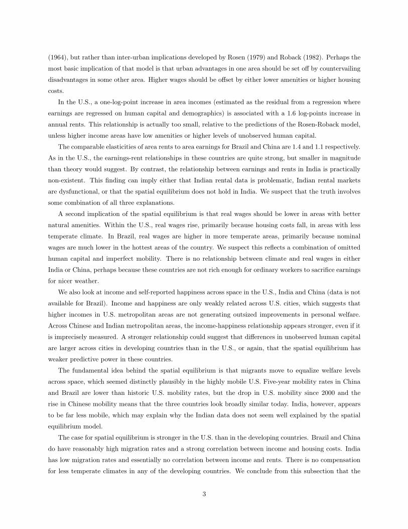
China lies between these two extremes. Figure 1 shows that the paths of urbanization (as defined by the
percentage of the population living in what each national statistics office calls “urban areas”) also differ across
the countries. In 1965, Brazil was already one-half urban, while India and China were overwhelmingly rural.
Figure 1: Share of total population living in urban areas, 1960-2014
China
India
Brazil
USA
20
40
60
80
100
Urb
an P
opula
tion (
% o
f to
tal)
1960 1965 1970 1975 1980 1985 1990 1995 2000 2005 2010 2015
Source: World Development Indicators, The World Bank.
Brazil’s high level of urbanization was part of the classic 1960s puzzle of high Latin American urbanization.
Social scientists noted that “Latin America, on the whole, is more urbanized than it is industrialized or
developed in other respects” (Durand and Pelaez, 1965), and that “urbanization is occurring without any
industrialization” (Arriaga, 1968). While American per capita GDP was $7500 (in 2012 dollars) in the 1920s,
when the U.S. became 50 percent urban, Brazilian per capita GDP only reached that level in 2011, when it
was 80 percent urban. Indeed, today Brazil is more urbanized than the United States despite being far less
wealthy.
By contrast, India’s urbanization has shown a slow but steady growth from 18 percent in 1960 to 31
percent in 2010. India is still predominantly poor and predominantly rural. Yet India’s vast size means that
it has extensive mega-cities, despite having a low urbanization rate.
Before 1800, China had the globe’s greatest track record of city building, yet despite that history China’s
urbanization rate remained below 20 percent when Mao died in 1976. After that point, and the economic
opening that came with Deng Xiaoping’s Southern Strategy, China’s urbanization rate exploded. Chinese
income and urbanization levels are now far higher than those in India. China has even more vast cities,
most of whom westerners – even western urbanists– cannot name. According to the OECD (2015), in 2010
there were 643 million Chinese living in 127 metropolitan areas with more than 1.5 million people. By
contrast, there are only 11 such metropolitan areas all together in the United Kingdom, France, Belgium,
6
the Netherland, Spain, Portugal and Switzerland (OECD, 2012).
Defining Agglomerations
In order to produce results comparable to U.S. urban research, we need to define comparable geographic
units. Even more challenging, we will need to define geographic units that can be identified in large data sets
with individual-level information. Typically, U.S. research uses metropolitan areas, which are multi-county
agglomerations, defined by the U.S. Census. Since the Census definitions change, we follow the convention of
using the definitions as of 2010 and using Consolidated Metropolitan Statistical Areas, which are relatively
large groupings. The U.S. Census considers all Americans who live within metropolitan areas to be urban,
since they are part of a large urban labor market, even if their own home is surrounded by considerable
greenery.
The OECD (2012) and other organizations have already defined functional urban units for a large number
of countries, and for many purposes it would be better to simply use their definitions. Yet our purpose is to
replicate the U.S. urban literature, which uses individual level-data and, as such, we must also use Brazilian,
Chinese and Indian censuses and surveys containing large numbers of individuals. These data sources don’t
use OECD urban area definitions, and typically contain geographic identifiers based on political boundaries.
We will define metropolitan areas using those boundaries, typically excluding non-urban respondents both
from our tests and from our definition of area-level variables, such as aggregate population, density and skill
levels.
In the case of Brazil we use microregions, which are agglomerations of contiguous and economically inte-
grated municipalities that have similar economic features, defined by the Brazilian Institute for Geography
and Statistics (IBGE, 2002). These areas capture better the notion of local labor markets than munici-
palities, which are more similar to U.S. counties in that they can differ dramatically in size and economic
characteristics. Using legally defined metropolitan regions was not a plausible alternative either, because
the Brazilian constitution of 1988 delegates to the states the right to establish them, and the criteria used
to form these regions varies significantly across states.
For China we use administrative “cities”, including provincial-level and prefecture-level areas. The name
can be misleading, since these geographical units are typically regions that comprise both urban and rural
territories. While there is not a single spatial administrative structure for cities, a typical “large” city
(provincial or prefecture level) includes both an urban core and large rural areas with scattered towns. The
urban core and its surroundings are in turn divided into districts, and the rural areas into “counties” (Chan,
2007).
In the case of India we use districts, the second-level administrative division of the country after states and
union territories. This choice enables us to merge the available microdata to area-level aggregates available
from the Indian Census and other sources. However, Indian districts are, for the most, geographically
extensive areas that contain large numbers of rural dwellers.
In order to make the units of analysis from Brazil, China and India more comparable to those from the
7
U.S., we restrict the samples to urban individuals and urban-only area aggregates throughout most of the
study. Moreover, we try to homogenize the sample compositions by restricting them to the higher end of
the urban population distributions (areas with 100,000 urban dwellers or more).
Like U.S. definitions of metropolitan areas, the boundaries of Brazilian microregions, Chinese cities and
Indian districts change over time. In these large developing countries, the process is mostly driven by the
breakup of existing administrative units to create smaller ones. Thus, we need to construct time-consistent
geographies for the cases where we perform inter-temporal comparisons.
In the case of Brazil, we employ data from municipality-level border changes for the period 1980-2010
to aggregate microregions when necessary and construct time-consistent borders following Kovak (2013). In
the cases of China and India, we use GIS historical data to geo-match current borders to 1980 borders, and
use the 1980 area definitions aggregating smaller areas when necessary.
We recognize that our definitions are debatable, but we believe that these are reasonable choices with
the goal of creating a standard definition across quite different countries.
The Distribution of Populations across Area Sizes
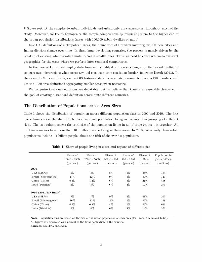
Table 1 shows the distribution of population across different population sizes in 2000 and 2010. The first
five columns show the share of the total national population living in metropolitan grouping of different
sizes. The last column shows the total size of the population living in all of these groups put together. All
of these countries have more than 100 million people living in these areas. In 2010, collectively these urban
populations include 1.4 billion people, about one fifth of the world’s population.
Table 1: Share of people living in cities and regions of different size
Places of Places of Places of Places of Places of Population in100K – 250K 250K – 500K 500K – 1M 1M – 1.5M 1.5M+ places 100K+
(percent) (percent) (percent) (percent) (percent) (millions)
2000USA (MSAs) 5% 8% 8% 6% 38% 184Brazil (Microregions) 17% 12% 9% 5% 30% 123China (Cities) 0.3% 1.2% 6% 8% 21% 458India (Districts) 2% 5% 6% 4% 10% 279
2010 (2011 for India)USA (MSAs) 5% 7% 9% 5% 41% 207Brazil (Microregions) 16% 12% 11% 6% 32% 148China (Cities) 0.2% 0.8% 4% 6% 39% 669India (Districts) 2% 4% 6% 4% 14% 373
Note: Population bins are based on the size of the urban population of each area (for Brazil, China and India).All figures are expressed as a percent of the total population in the country.Sources: See data appendix.
8
The U.S. population distribution is heavily skewed towards the larger metropolitan areas, with 38 percent
of the population in such areas in 2000 and 41 percent in 2010. Collectively the other four population
groupings contain only 26 percent of the U.S. population in 2010.
Brazil also has a large share of its population (32 percent in 2010) in the largest metropolitan areas,
but it also has a large share in the smaller areas. Twenty-eight percent of the Brazilian urban population
lives in microregions with fewer than 500,000 inhabitants. Some of these smaller areas might not even be
classified as metropolitan areas within the U.S. We highlight this to emphasize that the data issues make
these comparisons challenging, especially when we are dealing with the less populated areas.
By contrast, only one percent of Chinese in 2010 live in cities of less than 500,000 and 39 percent of Chinese
live in metropolitan areas with more than 1.5 million people. While definitional issues might explain some
of the absence of smaller Chinese agglomerations, there is no doubt that a large number of Chinese live
in extremely large metropolitan areas. Perhaps the most striking fact is that between 2000 and 2010, the
share of Chinese living in such areas increased by 18 percent, which reflects both migration and the rapidly
expanding populations of many Chinese mega-cities.
Even in India, the share of the population living in the largest urban areas increased significantly between
2000 and 2010 – from ten percent to fourteen percent. India may be the least urbanized country in the
group, but it has 373 million urbanites living in cities with more than 100 thousand people, according to
our classification. This represents the second largest urban population in the world. The typical urbanite in
2010 is far more likely to reside in Beijing or Shanghai or Sao Paulo than in London or New York.
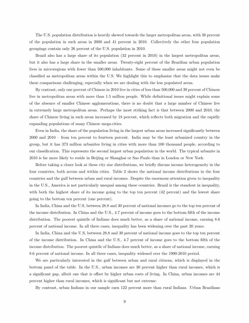
Before taking a closer look at these city size distributions, we briefly discuss income heterogeneity in the
four countries, both across and within cities. Table 2 shows the national income distributions in the four
countries and the gulf between urban and rural incomes. Despite the enormous attention given to inequality
in the U.S., America is not particularly unequal among these countries. Brazil is the standout in inequality,
with both the highest share of its income going to the top ten percent (42 percent) and the lowest share
going to the bottom ten percent (one percent).
In India, China and the U.S, between 28.8 and 30 percent of national incomes go to the top ten percent of
the income distribution. In China and the U.S., 4.7 percent of income goes to the bottom fifth of the income
distribution. The poorest quintile of Indians does much better, as a share of national income, earning 8.6
percent of national income. In all three cases, inequality has been widening over the past 20 years.
In India, China and the U.S, between 28.8 and 30 percent of national income goes to the top ten percent
of the income distribution. In China and the U.S., 4.7 percent of income goes to the bottom fifth of the
income distribution. The poorest quintile of Indians does much better, as a share of national income, earning
8.6 percent of national income. In all three cases, inequality widened over the 1990-2010 period.
We are particularly interested in the gulf between urban and rural citizens, which is displayed in the
bottom panel of the table. In the U.S., urban incomes are 30 percent higher than rural incomes, which is
a significant gap, albeit one that is offset by higher urban costs of living. In China, urban incomes are 44
percent higher than rural incomes, which is significant but not extreme.
By contrast, urban Indians in our sample earn 122 percent more than rural Indians. Urban Brazilians
9
earn 176 percent more than the rural Brazilians. These gulfs are enormous, suggestive of huge productivity
differences between urban and rural areas. Presumably, a significant fraction of these gulfs reflect unobserved
and observed human capital characteristics (Young, 2013), and perhaps also non-pecuniary compensation in
rural areas. Given the enormous differences between rural and urban Brazil and India, we will include only
urbanites in the tests that follow. Nonetheless, we will still have to grapple with unusually large earnings
differences across space that do not seem to be fully offset by differences in housing costs.
Table 2: Income distributions, 1990-2010
USA Brazil
1990 2000 2010 1991 2000 2010National income distributionIncome share held by lowest 20% 5.4% 5.4% 4.7% 2.3% 2.4% 3.3%Income share held by second 20% 11.2% 10.7% 10.4% 5.5% 5.9% 7.5%Income share held by third 20% 16.7% 15.7% 15.8% 9.7% 10.3% 12.3%Income share held by fourth 20% 23.7% 22.4% 23.1% 17.9% 18.0% 19.4%Income share held by highest 20% 43.1% 45.9% 46.0% 64.6% 63.4% 57.6%
Income share held by lowest 10% 1.8% 1.8% 1.4% 0.8% 0.7% 1.0%Income share held by highest 10% 26.7% 29.9% 29.6% 48.1% 47.3% 41.9%
Income levels (in 2014 $, PPP) Income per capita Income per capita
1990 2000 2010 1991 2000 2010Urban Areas 37,195 44,071 45,124 3,899 5,830 7,543Rural areas 26,816 31,342 34,835 1,141 1,846 2,731Difference 10,379 12,729 10,289 2,758 3,984 4,812
China India
1990 1999 2010 1993 2004 2009National income distributionIncome share held by lowest 20% 8.0% 6.4% 4.7% 9.1% 8.6% 8.6%Income share held by second 20% 12.2% 10.3% 9.7% 12.8% 12.2% 12.1%Income share held by third 20% 16.5% 15.0% 15.3% 16.5% 15.8% 15.7%Income share held by fourth 20% 22.6% 22.2% 23.2% 21.5% 21.0% 20.8%Income share held by highest 20% 40.7% 46.1% 47.1% 40.1% 42.4% 42.8%
Income share held by lowest 10% 3.5% 2.7% 1.7% 4.0% 3.8% 3.7%Income share held by highest 10% 25.3% 29.7% 30.0% 26.0% 28.2% 28.8%
Income levels (in 2014 $, PPP) Income per capita Earnings per capita
1990 1999 2010 2005 2011Urban Areas 1,451 3,064 6,179 3,123 5,027Rural areas 660 1,099 4,265 1,129 2,265Difference 792 1,965 1,914 1,994 2,762
Sources: See data appendix.
10
III. City Size Distributions: Zipf’s Law and Gibrat’s Law
Before discussing facts related to economic theories, we follow Rosen and Resnick (1980) and Soo (2005) and
turn to two stylized facts about city size distributions: Zipf’s Law and Gibrat’s Law. We choose to begin
here despite the large international literature on these laws (e.g. Rose, 2006; Soo, 2014), because we are using
slightly different city size definitions and because it is important to duplicate past results using our attempt
at producing consistent data. Zipf’s Law was originally posed as the rank size rule: the population of the
Nth largest city is 1/N times the population of the largest city. In large samples, this claim is equivalent to
the city size distribution being characterized by a power law distribution with a coefficient of minus one.
Gibrat’s Law is dynamic. It states that the growth rate of population is unrelated to the initial population.
Researchers typically test Gibrat’s Law by regressing the change in the logarithm of city population on
the initial level of city population, and testing whether the coefficient is statistically distinct from zero.
Champernowne (1953) and Gabaix (1999) linked the two facts and showed that if Gibrat’s Law holds
for city growth rates, then the equilibrium distribution of city sizes will display Zipf’s Law. This result is
mathematical, not economic, and it requires no assumptions about the motives of migrants or the productivity
of firms.
Our purpose is not to revisit the many controversies around Zipf’s Law (e.g. Holmes and Lee, 2010) or the
methodological issues related to measurement. We will use the simplest established techniques and compare
across countries. We will also use our measures of metropolitan area population, which are also debatable.
Throughout this paper, we aim to reproduce simple, transparent facts about space, not to advance methods
or debate nuanced issues within the established literature.
Zipf’s Law across Four Countries
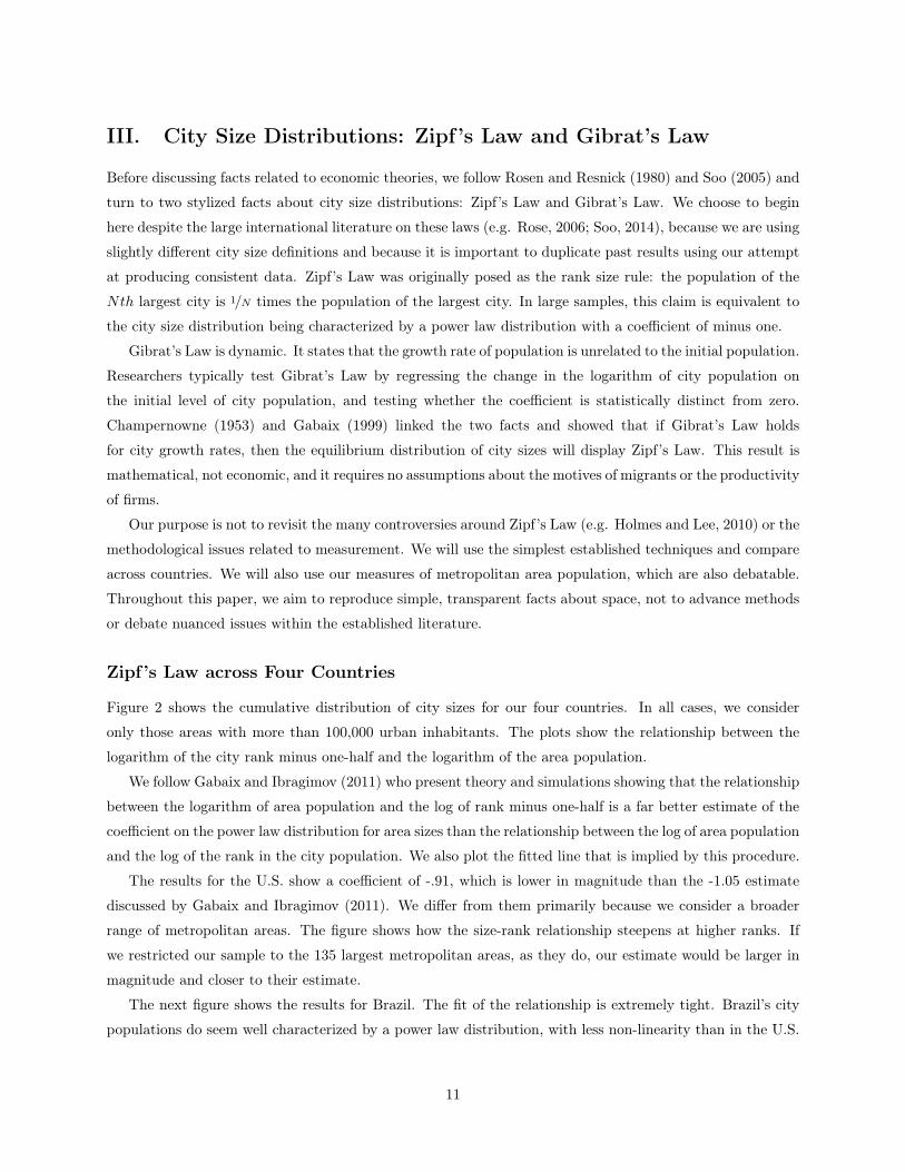
Figure 2 shows the cumulative distribution of city sizes for our four countries. In all cases, we consider
only those areas with more than 100,000 urban inhabitants. The plots show the relationship between the
logarithm of the city rank minus one-half and the logarithm of the area population.
We follow Gabaix and Ibragimov (2011) who present theory and simulations showing that the relationship
between the logarithm of area population and the log of rank minus one-half is a far better estimate of the
coefficient on the power law distribution for area sizes than the relationship between the log of area population
and the log of the rank in the city population. We also plot the fitted line that is implied by this procedure.
The results for the U.S. show a coefficient of -.91, which is lower in magnitude than the -1.05 estimate
discussed by Gabaix and Ibragimov (2011). We differ from them primarily because we consider a broader
range of metropolitan areas. The figure shows how the size-rank relationship steepens at higher ranks. If
we restricted our sample to the 135 largest metropolitan areas, as they do, our estimate would be larger in
magnitude and closer to their estimate.
The next figure shows the results for Brazil. The fit of the relationship is extremely tight. Brazil’s city
populations do seem well characterized by a power law distribution, with less non-linearity than in the U.S.
11
However, the -1.18 estimated coefficient is much higher than in the U.S. and higher than predicted by Zipf’s
Law. This high coefficient means that population rises too slowly as rank falls, or that Brazil’s biggest cities
are smaller than Zipf’s Law would predict. Soo (2014) finds an estimate of .94 for Brazil across his entire
sample, but the coefficient rises as he restricts the sample to larger cities. Rose (2006) found a coefficient of
-1.23 for Brazil which is quite close to our estimate.
Figure 2: Zipf’s Law. Urban populations and urban population ranks, 2010USA Brazil
−2
02
46
8L
og
of
shift
ed
ra
nk
(ra
nk−
1/2
), 2
01
0
11 13 15 17Log of urban population
Regression: Log(Rank−1/2) = 19.45 ( 0.00) −1.18 ( 0.00) Log Pop. (N=319; R2=0.995)
China India
Note: Regression specifications and standard errors based on Gabaix and Ibragimov (2011). Samples restricted to areaswith urban population of 100,000 or larger.Sources: See data appendix.
The third figure shows results for China, following Anderson and Ge (2005). The estimated coefficient
of -.91 seems reassuringly close to the U.S., but the figure suggests that such comfort is mistaken. The
-.91 coefficient masks strong non-linearity in the rank-size relationship, and the r-squared is quite low (.79)
relative to the U.S. (.94) or Brazil (.99). The steep curve among the larger Chinese cities suggests that when
it comes to big areas, China is more like Brazil than like the U.S. China also has far fewer extremely large
cities than Zipf’s Law would suggest. The -.91 estimate is larger in magnitude than Soo (2014), but smaller
than Schaffar and Dimou (2012) and Rose (2006).
12
The final panel shows results for India, which has -1.03 coefficient, suggesting that Zipf’s Law appears to
work for Indian cities even more strongly than it does in the U.S. This estimate is close to Soo (2005) but
less than Rose (2006). Our r-squared (.92) is somewhat lower than the U.S. and there is also some concavity
in the relationship between rank and size, suggesting that there are again fewer large cities than Zipf’s Law
would suggest.
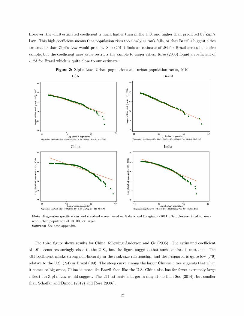
In Table 3, we test whether the city size distributions are the same across the four countries. The top
panel in the table shows results for all city sizes. The bottom panel shows results only for city sizes above
500,000, where we are more confident that metropolitan area definitions are not driving the results.
Table 3: Urban population Kolmogorov–Smirnov two-sample tests
Brazil China India(Microregions) (Cities) (Districts)
Full Sample
USA (MSAs) 0.396 0.534 0.194(0.000) (0.000) (0.000)
Brazil (Microregions) 0.779 0.346(0.000) (0.000)
China (Cities) 0.564(0.000)
Cities with urban population of 500,000 or more
USA (MSAs) 0.148 0.229 0.123(0.432) (0.001) (0.286)
Brazil (Microregions) 0.342 0.085(0.000) (0.911)
China (Cities) 0.301(0.000)
Note: Figures are D test-statistic scores, p-values in parentheses. Theobservations in the full sample are: US = 258, Brazil = 548, China = 345and India = 632. The observations in the restricted sample are: US = 93,Brazil = 55, China = 296 and India = 204.Sources: See data appendix.
The table reports D statistics from two-sample Kolmogorov-Smirnov tests that compare each pair of
city size distributions. For the whole sample of cities, for every pair of countries we can reject that the
distributions are identical. China’s city size distribution is particularly distinct statistically, with all D
statistics above .5. India and the U.S. appear to have the most similar city size distributions, with a D
statistics less than .2.
When we turn only to the larger metropolitan areas, the differences become muted. The U.S., Brazilian
and Indian city size distributions are no longer statistically distinct. China’s city size distribution is, however,
statistically different from the other three. The primary difference is again that China has fewer ultra-large
13
cities than the U.S. city size distribution would predict if it was applied to the number and total population
of Chinese cities.
There are many possible explanations for these differences. China’s population has exploded so rapidly
that it may be far from steady state. China’s governments are far more active in planning city populations
than any of the other countries. The growth of ultra large Chinese cities may also be blocked by disamenities
of size that can become extreme for urban populations over 20 million. Finally, both China and India may
be better seen as continents rather than standard countries and this may also explain some of the difference.
The differences between China and the other countries does raise the possibility that in the long run
China’s urban populations will be much more skewed towards ultra large areas like Beijing and Shanghai.
The attempts of many local governments to boost growth in middle size (Tier 3 and Tier 4) cities seem to
have led to fiscal difficulties. Over time, more vertical construction and congestion pricing may ease the
disamenities of crowding and congestion. China’s city size distribution may eventually look far more like
Zipf’s Law, and to examine that possibility we now turn to the dynamics of city growth and Gibrat’s Law.
Gibrat’s Law across Four Countries
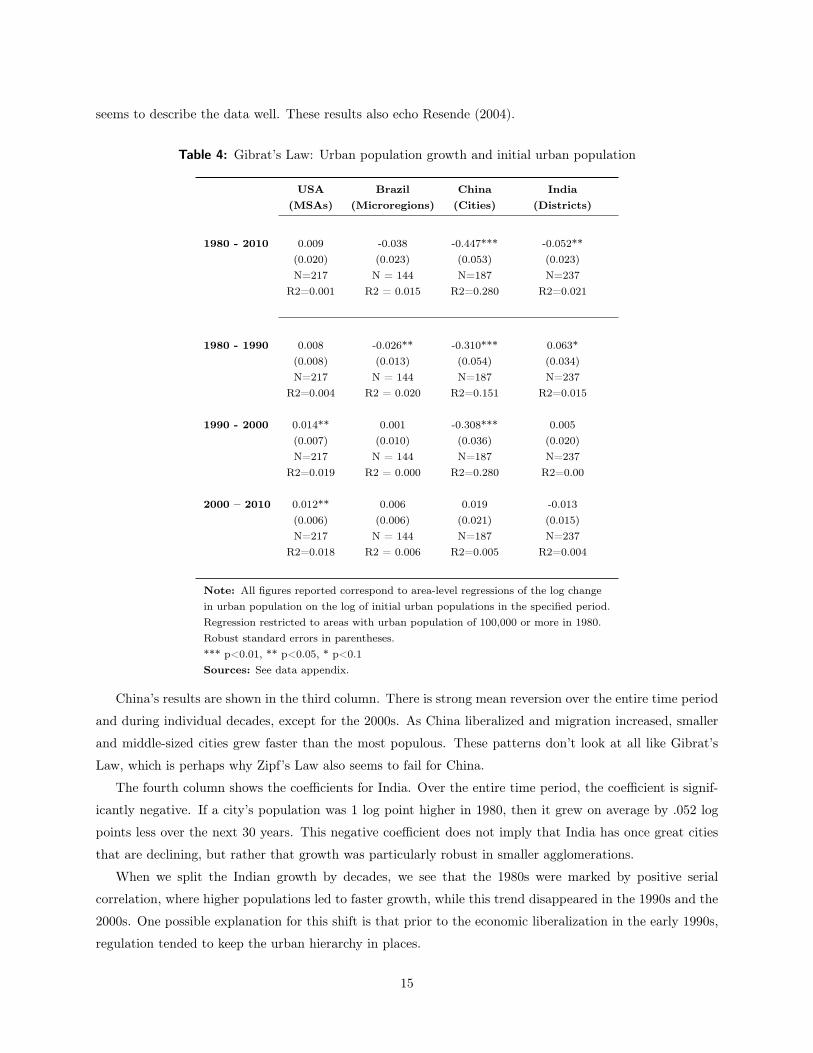
Table 4 shows our results on the mean reversion of city populations. In all cases, we report coefficients where
the change in the logarithm of area urban population is regressed on the logarithm of initial area urban
population. Gibrat’s Law implies that the coefficient should be statistically indistinguishable from zero.
The first column shows results for the United States for 1980-2010. We first show the coefficient for
the entire time period and then results for each of the three decades separately. Over the entire 1980-2010,
there is no correlation between initial population and subsequent population growth. The r-squared in the
regression is 0 to two decimal places. The estimated coefficient is .009. The standard error around that
coefficient means that we cannot rule out the possibility that the coefficient is .03, but even that coefficient
is quite small for a thirty-year period.
Gibrat’s Law holds less perfectly within the U.S. during each independent decade. In both the 1990s
and the 2000s, the estimated coefficient is close to .01 and statistically significant. Yet given the strong
correlation that exists between metropolitan area growth and other variables, such as January temperature
and education, these coefficients are quite compatible with Gibrat’s Law.
Gibrat’s Law has failed during many periods of U.S. history. Glaeser, Ponzetto and Tobio (2014b) examine
population growth among eastern counties of the U.S. from 1860 until today. For example, during the 1970s,
there was sharp mean reversion in population levels in those counties. During the 1960s, population growth
was much faster in more populous counties. Gibrat’s Law has not been a permanent feature of U.S. urban
dynamics, and perhaps it should not be expected to hold in countries experiencing far more rapid urban
change.
The second column shows the results for Brazil, which are generally statistically indistinguishable from
the U.S. Over the entire time period, like Soo (2014), we cannot reject the hypothesis that Gibrat’s law holds
in Brazil. During the 1980s, there was slight mean reversion, but during the 1990s and 2000s, Gibrat’s Law
14
seems to describe the data well. These results also echo Resende (2004).
Table 4: Gibrat’s Law: Urban population growth and initial urban population
USA Brazil China India(MSAs) (Microregions) (Cities) (Districts)
1980 - 2010 0.009 -0.038 -0.447*** -0.052**(0.020) (0.023) (0.053) (0.023)N=217 N = 144 N=187 N=237
R2=0.001 R2 = 0.015 R2=0.280 R2=0.021
1980 - 1990 0.008 -0.026** -0.310*** 0.063*(0.008) (0.013) (0.054) (0.034)N=217 N = 144 N=187 N=237
R2=0.004 R2 = 0.020 R2=0.151 R2=0.015
1990 - 2000 0.014** 0.001 -0.308*** 0.005(0.007) (0.010) (0.036) (0.020)N=217 N = 144 N=187 N=237
R2=0.019 R2 = 0.000 R2=0.280 R2=0.00
2000 – 2010 0.012** 0.006 0.019 -0.013(0.006) (0.006) (0.021) (0.015)N=217 N = 144 N=187 N=237
R2=0.018 R2 = 0.006 R2=0.005 R2=0.004
Note: All figures reported correspond to area-level regressions of the log changein urban population on the log of initial urban populations in the specified period.Regression restricted to areas with urban population of 100,000 or more in 1980.Robust standard errors in parentheses.*** p<0.01, ** p<0.05, * p<0.1Sources: See data appendix.
China’s results are shown in the third column. There is strong mean reversion over the entire time period
and during individual decades, except for the 2000s. As China liberalized and migration increased, smaller
and middle-sized cities grew faster than the most populous. These patterns don’t look at all like Gibrat’s
Law, which is perhaps why Zipf’s Law also seems to fail for China.
The fourth column shows the coefficients for India. Over the entire time period, the coefficient is signif-
icantly negative. If a city’s population was 1 log point higher in 1980, then it grew on average by .052 log
points less over the next 30 years. This negative coefficient does not imply that India has once great cities
that are declining, but rather that growth was particularly robust in smaller agglomerations.
When we split the Indian growth by decades, we see that the 1980s were marked by positive serial
correlation, where higher populations led to faster growth, while this trend disappeared in the 1990s and the
2000s. One possible explanation for this shift is that prior to the economic liberalization in the early 1990s,
regulation tended to keep the urban hierarchy in places.
15
Brazil and the U.S. both appear to adhere broadly to both Zipf’s and Gibrat’s Laws. China and India do
not. Perhaps the most natural reason why Brazil and the U.S. are similar is that they are both moderately
sized places, which have long been largely urban. China and India are both much larger, and many of their
cities are much newer. If they have not reached a dynamic steady state, then perhaps Gibrat’s and Zipf’s
Laws may eventually appear in their urban systems.
IV. The Spatial Equilibrium
We now turn to empirical tests that are motived by economics. For over fifty years, the spatial equilibrium
has been the organizing principle of urban economics. It was first applied to land prices and land usages
within the metropolitan areas by Alonso (1964) and Muth (1969) and then it was applied to income and
price differences across metropolitan areas by Rosen (1979) and Roback (1982). The core idea of the spatial
equilibrium is that locations don’t offer a free lunch. If a place has high wages and decent amenities, then
real estate costs should be high. If a place has nice amenities, then real wages (i.e. wages controlling for
local prices) should be lower.
We look at four different empirical patterns that are related to the spatial equilibrium. We begin by
testing whether the costs of living rise with wages across metropolitan areas. We then test whether real
wages are lower in places that have more attractive natural climates. Third, we examine whether self-
reported life satisfaction is higher in places with higher income and we end this section by looking at overall
migration patterns. Migration is not itself a prediction of the spatial equilibrium model, but it is one channel
through which the spatial equilibrium is produced. When migration is low, we might be less confident about
the predictions of the spatial equilibrium model.
The first three tests all try to assess whether people in one area are receiving a higher welfare level than
people in another area. But if these tests fail, then there are always two quite plausible explanations. First,
a spatial equilibrium might not exist because of legal or preference based barriers to mobility. Second, the
people in the more successful area might have fundamentally different levels of unobserved human capital
than the people in the less successful area. If the two areas have very different people, then we would not
expect them to deliver the same welfare levels. While we can control for observable human capital measures,
such as years of schooling, we can never reject the possibility that unobserved human capital is driving our
results.
The Relationship between Prices and Wages
The starting point for the spatial equilibrium is the assumption that utility is equalized over space for any
homogenous set of workers who are living in multiple cities. Individual heterogeneity can come in the form of
place-independent heterogeneity, such as different levels of human capital or tastes for particular amenities,
or place-dependent heterogeneity, such as taste for living in a particular locale. Both types of heterogeneity
can be modeled. For example, Glaeser (2008) discusses models of heterogeneous worker human capital.
16
Diamond (2015) works with heterogeneous tastes for cities, as well as heterogeneous human capital. For
expositional purposes, we will stick with the most standard and simple assumption of worker homogeneity.
In this case, we can define an indirect utility function over wages, prices and amenties V ((1� t)W,P,A),
where (1� t)W reflects after-tax wages, P reflects prices and A reflects amenities. This indirect utility
function is typically either operationalized as a log-separable or a linear-separable function. The log-separable
function is justified by a Cobb-Douglas utility function defined over a general consumption good and housing.
This can produce an indirect utility function of A (1� t)WP
�↵, where A represents an index of amenity
values which is assumed to multiply welfare and ↵ represents the share of housing in the utility function and
household spending.
The linear-separable structure is justified by assuming that every person consumes exactly one unit of
housing and, consequently, people’s after-housing income is W � P . In the linear separable formulation, it
is convenient to assume that the amenity index is just added to net earnings so that total welfare is just
(1� t)W � P + A. In the log-separable formulation, nation-wide proportional taxes are irrelevant to the
relationship between wages and prices. In the linear-separable formulation, nation-wide proportional taxes
will matter, unless housing costs are deductible. In the U.S., housing prices are partially deductible because
of the home mortgage interest deduction.1
The log-separable formulation suggests the relationship:
Log (Price) =1
↵
(Log (Wage) + Log (Amenities)) (1)
The linear-separable formulation suggests:
Price = After TaxWage+Amenities (2)
If log price is regressed on log wages, then the first formulation implies that the coefficient will be1↵
⇣1 + Cov(Log(Wage),Log(Amenities))
V ar(Log(Wage))
⌘. As the historic share of spending that goes towards housing is ap-
proximately one-third, this suggests a benchmark coefficient of three. The second formulation suggests that
if price is regressed on wage, the coefficient will be 1� t+ Cov(Wage,Amenities)V ar(Wage) . The two models yield tight
predictions only if we know the correlation of the amenity index and wages, which we unfortunately do not.
Our approach is not to attempt to definitively disprove the spatial equilibrium predictions, but rather to
test whether reality is roughly compatible with the predictions of the model in our four countries.
An added complication is that measured wages and measured housing prices will necessarily vary because
of differences in human capital and the physical characteristics of the house. Our approach to this issue is to
estimate a wage residual from a regression in which the logarithm of wages is regressed on individual human
capital characteristics, including years of schooling and age. To promote comparability, we will only include
males in this wage regression. We will then include this residual in a regression in which housing cost is
regressed on this area-level wage and other housing characteristics, especially the physical characteristics of
1Albuoy (2015) provides a comprehensive discussion of the connection between deductibility and the spatial equilibrium.
17
the home.
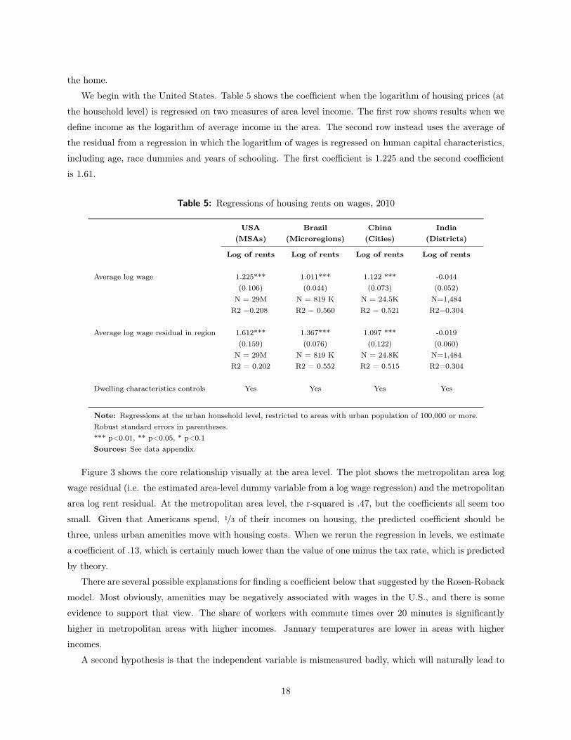
We begin with the United States. Table 5 shows the coefficient when the logarithm of housing prices (at
the household level) is regressed on two measures of area level income. The first row shows results when we
define income as the logarithm of average income in the area. The second row instead uses the average of
the residual from a regression in which the logarithm of wages is regressed on human capital characteristics,
including age, race dummies and years of schooling. The first coefficient is 1.225 and the second coefficient
is 1.61.
Table 5: Regressions of housing rents on wages, 2010
USA Brazil China India(MSAs) (Microregions) (Cities) (Districts)
Log of rents Log of rents Log of rents Log of rents
Average log wage 1.225*** 1.011*** 1.122 *** -0.044(0.106) (0.044) (0.073) (0.052)
N = 29M N = 819 K N = 24.5K N=1,484R2 =0.208 R2 = 0.560 R2 = 0.521 R2=0.304
Average log wage residual in region 1.612*** 1.367*** 1.097 *** -0.019(0.159) (0.076) (0.122) (0.060)
N = 29M N = 819 K N = 24.8K N=1,484R2 = 0.202 R2 = 0.552 R2 = 0.515 R2=0.304
Dwelling characteristics controls Yes Yes Yes Yes
Note: Regressions at the urban household level, restricted to areas with urban population of 100,000 or more.Robust standard errors in parentheses.*** p<0.01, ** p<0.05, * p<0.1Sources: See data appendix.
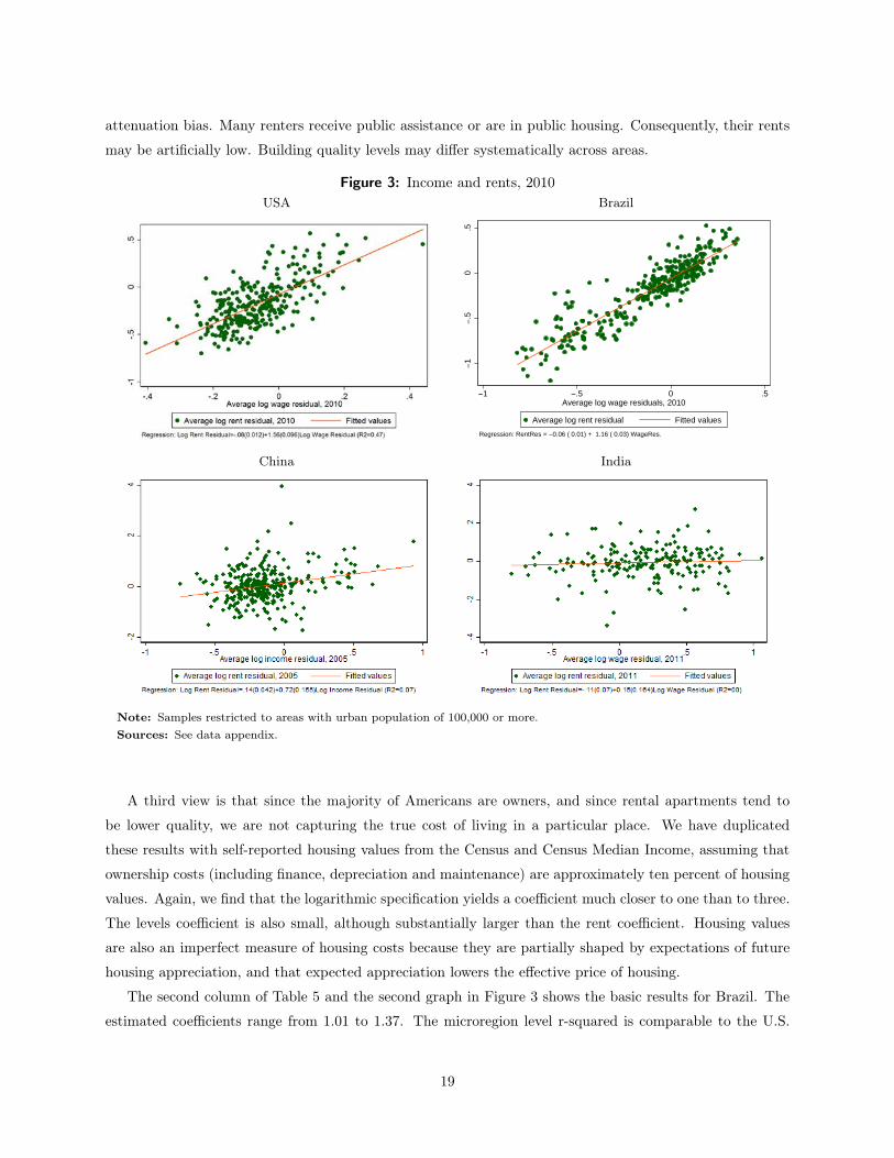
Figure 3 shows the core relationship visually at the area level. The plot shows the metropolitan area log
wage residual (i.e. the estimated area-level dummy variable from a log wage regression) and the metropolitan
area log rent residual. At the metropolitan area level, the r-squared is .47, but the coefficients all seem too
small. Given that Americans spend, 1/3 of their incomes on housing, the predicted coefficient should be
three, unless urban amenities move with housing costs. When we rerun the regression in levels, we estimate
a coefficient of .13, which is certainly much lower than the value of one minus the tax rate, which is predicted
by theory.
There are several possible explanations for finding a coefficient below that suggested by the Rosen-Roback
model. Most obviously, amenities may be negatively associated with wages in the U.S., and there is some
evidence to support that view. The share of workers with commute times over 20 minutes is significantly
higher in metropolitan areas with higher incomes. January temperatures are lower in areas with higher
incomes.
A second hypothesis is that the independent variable is mismeasured badly, which will naturally lead to
18
attenuation bias. Many renters receive public assistance or are in public housing. Consequently, their rents
may be artificially low. Building quality levels may differ systematically across areas.
Figure 3: Income and rents, 2010USA Brazil
−1
−.5
0.5
−1 −.5 0 .5Average log wage residuals, 2010
Average log rent residual Fitted values
Regression: RentRes = −0.06 ( 0.01) + 1.16 ( 0.03) WageRes.
China India
Note: Samples restricted to areas with urban population of 100,000 or more.Sources: See data appendix.
A third view is that since the majority of Americans are owners, and since rental apartments tend to
be lower quality, we are not capturing the true cost of living in a particular place. We have duplicated
these results with self-reported housing values from the Census and Census Median Income, assuming that
ownership costs (including finance, depreciation and maintenance) are approximately ten percent of housing
values. Again, we find that the logarithmic specification yields a coefficient much closer to one than to three.
The levels coefficient is also small, although substantially larger than the rent coefficient. Housing values
are also an imperfect measure of housing costs because they are partially shaped by expectations of future
housing appreciation, and that expected appreciation lowers the effective price of housing.
The second column of Table 5 and the second graph in Figure 3 shows the basic results for Brazil. The
estimated coefficients range from 1.01 to 1.37. The microregion level r-squared is comparable to the U.S.
19
metropolitan area sample. These results corroborate Azzoni and Servo (2002) who also find higher costs of
living in higher Brazilian regions.
The Brazilian figure should be larger than the U.S. figure because Brazilian spending on housing is
a smaller share of total income, approximately 15 percent according the Credit Suisse Survey Emerging
Consumer Survey. If that is correct, then the predicted log coefficient could be as high as seven. The same
explanations for the low estimate exist in Brazil as well as the U.S.: a negative amenity correlation with
high incomes and mismeasurement of both the dependent and independent variable.
Overall, though, the Rosen-Roback inspired wage-to-rent relationship looks pretty similar in the U.S.
and Brazil. In both cases, area-level rents are tightly correlated with area-level incomes. In both cases, the
coefficients are close to one, which is a far smaller relationship than is predicted by economic theory. The
similarities between the Brazilian and American results leave us optimistic that the tradition of Rosen-Roback
inspired hedonic regressions that has been so successful with U.S. data can proceed in Brazil.
The third column of Table 5 and the third graph in Figure 3 provide the results for China. The table’s
estimated coefficients are again close to one, which suggests that Chinese do pay more when incomes are
higher, as in Long, Guo and Zheng (2009). Nonetheless, the coefficient of one seems low, since the Chinese
spend an even smaller share of their incomes (ten percent) on housing than the Brazilians. The graph shows
that the r-squared of the relationship (.07) is much smaller than in the U.S. and Brazil. The goodness of fit
in the table and the figure can be quite different, because the table reflects individual-level data while the
figure looks at the area-level relationship, which is not weighted by the number of people in each area.
Chinese rents are correlated with incomes across areas, but the link is much weaker than either the U.S.
or Brazil. One explanation for this is that amenity correlation with income is even more negative and that
is certainly possible. Another possibility is the barriers to mobility in China, especially the famous Hukuo
system make it difficult for migration to equalize welfare levels.
Yet a third possibility is that public interventions in the housing market are particularly important in
China, and these act to distort market prices. Moreover, only 10 percent of Chinese and 13.4 percent
of Indians rent. A standard explanation for these low homeownership rates is that rental markets are
dysfunctional and distorted by rent-control-like rules. It is notable that speculators in Chinese real estate will
often buy apartments and leave them empty rather than taking the risk of renting them out. Consequently,
people are unable to rent and must buy low quality housing instead. The rental market that does exist may
only reflect a very unusual part of the housing market.
Finally, with those concerns in mind, we turn to the results from India. The last graph in Figure 3 shows
that there is essentially no correlation between income and rents across Indian regions. This non-result is
repeated in the fourth column in Table 5. Possibly, this non-correlation reflects profound amenity differences
across Indian cities, but it seems just as likely to reflect terrible measurement of housing rents. For example,
in many cases, landlords are not allowed to raise rents and cannot eject tenants. Indeed, it is hard to see
any pattern in our Indian rent data, which leads us to suspect that without better data on the cost of living,
any hedonic estimates pursued with this data are risky. Certainly, we cannot conclude that this provides
any support for the usefulness of the spatial equilibrium model in India.
20
Across the four countries, the patterns in Brazil and the U.S. were broadly similar. Both countries have
a tight correlation between income and rents. In both countries, the estimated relationship was smaller than
would be predicted by the core Rosen-Roback model. The link between income and rents was weaker in
China, but still significant. The link disappears entirely in India. For some reason, the spatial equilibrium
model appears to be least effective in the poorest nation, either because an equilibrium does not exist or
because measurement is most problematic. We now turn to the equilibrium pricing of amenities.
Real Wages and Amenities
Equations (1) and (2) also provide implications about the connection between amenities and real wages, where
real wages are defined either as Log (Wage)�↵Log (Price), in the logarithmic model or as Wage�Price, in
the linear model. When it comes to amenities, the models do not yield any implication about the magnitude
of the effect. That will depend upon consumer valuation of amenities. The model does, however, imply that
areas will positive amenities will have lower real wages.
We will focus on climate-related amenities, which have the advantage of being exogenous to the local
economy and generally well measured. In our samples, we will typically have a measure of January and July
temperatures and an average precipitation measure. For January and July temperature, we will transform the
variable by taking that absolute value of the difference between the average temperature and the equivalent
in Celsius of 70 degrees Fahrenheit (21.11 degrees Celsius). Consequently, the value can increase if the area
is either particularly hot or particularly cold. The choice of 70 degrees represents a middle ground within
the 65 to 75 degree range that is often discussed an ideal for human comfort. We recognize that this choice
is relatively arbitrary within this range. Our results are not particularly sensitive to minor perturbations in
the assumed bliss point for temperature.
Table 6 shows our results. The first panel shows the findings for wages, rents and real wages in the
U.S. We use three distinct measures of climate amenities. First, we use the absolute value of the difference
between the average temperature in summer and 21.11 degrees Celsius. Second, we use the absolute value
of the difference between the average temperature in winter and 21.11 degrees. Finally, we use the average
annual rainfall.
The first column shows that there is no relationship between wages and these variables, controlling for
our core human capital attributes (age, race and years of schooling). The second column shows that a ten
degree Celsius difference between temperatures in either the winter or the summer from idea temperature is
associated with an approximately five percent increase in real wages. Americans do seem to be paid more
when they live in less temperate climates. The third column shows that these differences are largely driven
by lower rents in less temperate areas. There are no effects of rainfall.
These climate relationships with rents and real wages are a prediction of the Rosen-Roback model that is
confirmed within the U.S. Do real wages rise with bad climates in the developing world? The second panel
in Table 6 shows the results for Brazil. Brazil has lower wages in places that have less ideal temperatures.
Nominal wages are higher in areas with more rain as well.
21
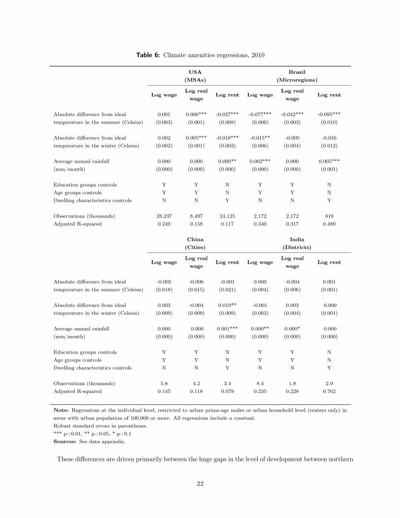
Table 6: Climate amenities regressions, 2010
USA Brazil(MSAs) (Microregions)
Log wageLog real
Log rent Log wageLog real
Log rentwage wage
Absolute difference from ideal 0.001 0.006*** -0.027*** -0.077*** -0.042*** -0.095***temperature in the summer (Celsius) (0.003) (0.001) (0.008) (0.006) (0.003) (0.010)
Absolute difference from ideal 0.002 0.005*** -0.018*** -0.015** -0.005 -0.016temperature in the winter (Celsius) (0.002) (0.001) (0.003) (0.006) (0.004) (0.012)
Average annual rainfall 0.000 0.000 0.000** 0.002*** 0.000 0.005***(mm/month) (0.000) (0.000) (0.000) (0.000) (0.000) (0.001)
Education groups controls Y Y N Y Y NAge groups controls Y Y N Y Y NDwelling characteristics controls N N Y N N Y
Observations (thousands) 28,237 8,497 24,125 2,172 2,172 819Adjusted R-squared 0.249 0.158 0.117 0.340 0.317 0.480
China India(Cities) (Districts)
Log wageLog real
Log rent Log wageLog real
Log rentwage wage
Absolute difference from ideal -0.005 -0.006 -0.001 0.000 -0.004 0.001temperature in the summer (Celsius) (0.018) (0.015) (0.021) (0.004) (0.006) (0.001)
Absolute difference from ideal 0.003 -0.004 0.019** -0.001 0.003 0.000temperature in the winter (Celsius) (0.009) (0.009) (0.009) (0.003) (0.004) (0.001)
Average annual rainfall 0.000 0.000 0.001*** 0.000** 0.000* 0.000(mm/month) (0.000) (0.000) (0.000) (0.000) (0.000) (0.000)
Education groups controls Y Y N Y Y NAge groups controls Y Y N Y Y NDwelling characteristics controls N N Y N N Y
Observations (thousands) 5.8 4.2 3.4 8.4 1.8 2.9Adjusted R-squared 0.145 0.118 0.079 0.235 0.228 0.762
Note: Regressions at the individual level, restricted to urban prime-age males or urban household level (renters only) inareas with urban population of 100,000 or more. All regressions include a constant.Robust standard errors in parentheses.*** p<0.01, ** p<0.05, * p<0.1Sources: See data appendix.
These differences are driven primarily between the huge gaps in the level of development between northern
22
and southern Brazil. There are large human capital differences between north and south which are assuredly
only imperfectly captured by our coarse control variables and which are correlated with the weather (Azzoni
et al., 2000). There are also differences in the level of capital stock and infrastructure. Other work (Mueller,
2005) finds that Brazilians do seem to value climate differences that are not correlated with region.
Finally, the third regression shows results with rents, which are indeed also lower in places with more
extreme weather. While these results are compatible with the Rosen-Roback framework, the coefficients
are not large enough to reverse the also negative relationship with wages and hence we have the anomalous
result that people in Brazil earn more in real terms when the climate is worse.
The patterns for China and India are almost identical. In almost all cases, there is almost no correlation
between climate and any of our variables. China’s economic divide runs east-to-west rather than north-to-
south, like Brazil, which may explain why there isn’t a large correlation between climate and nominal wages.
Overall, perhaps the most natural explanation is that the Chinese and the Indians are not wealthy enough
to be willing to pay a significant premium to live in places with more temperate climates. Liu and Shen
(2014) also find a far weaker relationship between climate and population growth in China than in the U.S.
Happiness across Space
Economists like Jeremy Bentham and John Stuart Mill argued that human beings both should and typically
do try to maximize pleasure and minimize pain. If they were right, then the modern economists’ concept
of utility should be synonymous with self-reported happiness or life satisfaction. Yet many if not most
economists now reject the Benthamite hedonist approach that equates happiness and welfare. Utility func-
tions, in their modern use, are simply rankings based on preferences. People may sensibly make decisions
that appear to lower their level of reported life satisfaction. Parents of young children, for example, typically
report lower levels of life satisfaction, perhaps because of enormous time costs in caring for infants (Mclana-
han and Adams, 1987). This does not mean that those parents have made a mistake. Having children may
be rational and increase utility even if it does not increase happiness.
Nonetheless, we follow Glaeser, Gottlieb and Ziv (2014a) in believing that happiness can be useful for
examining the spatial equilibrium even if happiness is not equivalent to utility. Heterogeneity in happiness
across space should provide a test of the spatial equilibrium model. Strong differences in happiness can
be taken as evidence against the spatial equilibrium. Given the difficulties in attributing heterogeneity in
self-reported happiness to small samples or local cultures, we focus on the narrower question of whether
happiness rises with income across areas.
If the spatial equilibrium holds, we expect to find little or no relationship between happiness and area
income. Indeed, happiness may be a proxy for certain urban amenities, and then the spatial equilibrium
might predict that happiness should be lower, not higher, in richer areas. If there is a positive relationship
between income and happiness across areas, then this suggests either that the spatial equilibrium doesn’t
hold, or that different people live in different cities, or that happiness is not capturing welfare.
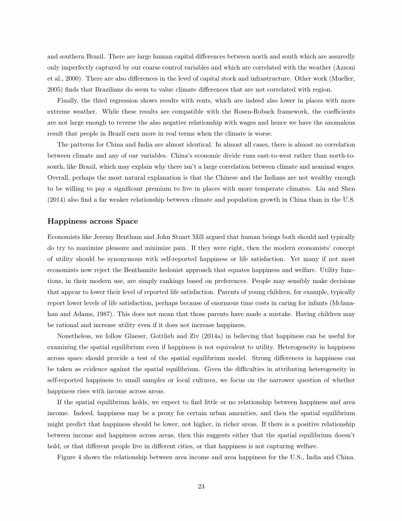
Figure 4 shows the relationship between area income and area happiness for the U.S., India and China.
23
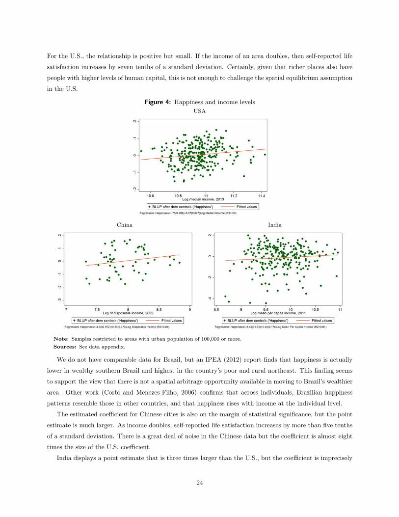
For the U.S., the relationship is positive but small. If the income of an area doubles, then self-reported life
satisfaction increases by seven tenths of a standard deviation. Certainly, given that richer places also have
people with higher levels of human capital, this is not enough to challenge the spatial equilibrium assumption
in the U.S.
Figure 4: Happiness and income levelsUSA
China India
Note: Samples restricted to areas with urban population of 100,000 or more.Sources: See data appendix.
We do not have comparable data for Brazil, but an IPEA (2012) report finds that happiness is actually
lower in wealthy southern Brazil and highest in the country’s poor and rural northeast. This finding seems
to support the view that there is not a spatial arbitrage opportunity available in moving to Brazil’s wealthier
area. Other work (Corbi and Menezes-Filho, 2006) confirms that across individuals, Brazilian happiness
patterns resemble those in other countries, and that happiness rises with income at the individual level.
The estimated coefficient for Chinese cities is also on the margin of statistical significance, but the point
estimate is much larger. As income doubles, self-reported life satisfaction increases by more than five tenths
of a standard deviation. There is a great deal of noise in the Chinese data but the coefficient is almost eight
times the size of the U.S. coefficient.
India displays a point estimate that is three times larger than the U.S., but the coefficient is imprecisely
24
measured so that we cannot statistically rule-out a coefficient smaller than the one in the U.S. It does seem
that richer cities are happier in the developing countries, more so than in the U.S., but the evidence is far
from conclusive.
There are at least two interpretations of these results that are quite compatible with the spatial equilib-
rium framework. One interpretation, again, is omitted human capital, and in that case, richer cities have
people who are richer because they are more skilled and we might expect them to have higher happiness
levels. Another interpretation is that happiness is reflecting urban amenities, which are higher in richer
places. In that second case, however, the failure to find much higher prices in high income areas in India
becomes even more of a puzzle.
The third explanation is that the spatial equilibrium assumption is just not particularly useful when
thinking about China, and especially India. Perhaps the most natural reason why the spatial equilibrium
assumption could fail is that mobility is limited, either because of strong tastes for remaining in places or
because of barriers to mobility like China’s Hukuo system. We now turn to facts about spatial mobility in
the four countries.
Mobility in the Four Countries
In principle, the spatial equilibrium does not require much mobility. Even if no one moves, housing costs can
adjust to keep welfare equal across space. However, immobility can be a sign that the assumptions needed
for the Rosen-Roback model do not hold. For example, if individuals were forbidden from moving across
state lines, then there would be no reason for utility levels to be equalized. Without labor mobility, regional
models revert to having the implications of national models, which certainly do not predict constant utility
across space.
In reality, mobility is possible but imperfect, and when immobility is caused by heterogeneity of tastes,
then the implications of the Rosen-Roback model weaken. Imagine if villagers have the option to move to a
city but they have tastes for living in the village of their youth and those tastes are heterogeneous. The real
wage gap between the village and the city will equal the taste for the village held by the marginal migrant.
Strong tastes will mean that the real wage gap can be quite large, and immobility is a sign that tastes for
one’s home are strong. Moreover, there are good reasons to believe that the limitations on mobility differ
across countries (Bell and Muhidin, 2009), which may explain the differences in the empirical value of the
spatial equilibrium concept.
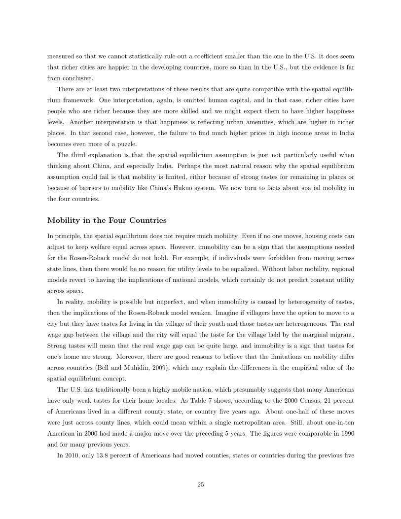
The U.S. has traditionally been a highly mobile nation, which presumably suggests that many Americans
have only weak tastes for their home locales. As Table 7 shows, according to the 2000 Census, 21 percent
of Americans lived in a different county, state, or country five years ago. About one-half of these moves
were just across county lines, which could mean within a single metropolitan area. Still, about one-in-ten
American in 2000 had made a major move over the preceding 5 years. The figures were comparable in 1990
and for many previous years.
In 2010, only 13.8 percent of Americans had moved counties, states or countries during the previous five
25
years. Only 7.1 percent had changed states or countries. While these figures are still relatively high by
global standards, they do represent a dramatic drop, which is presumably best understood as a reflection of
the Great Recession. Underwater homeowners may have been unable to sell their homes to move during the
downturn. Younger people often chose to stay at home during the recession to save costs.
Table 7: Percentage of the population living in a different locality five years ago
USA Brazil
1990 2000 2010 1991 2000 2010
Migrants in the last 5 years (% of population) 21.3% 21.0% 13.8% 9.5% 9.1% 7.1%From same state/prov., different county / dist. 9.7% 9.7% 6.7% 6.0% 5.4% 4.5%From different state/province 9.4% 8.4% 5.6% 3.5% 3.6% 2.4%From abroad 2.2% 2.9% 1.5% 0.04% 0.1% 0.14%
China India
2000 2010 1993 2001 2011
Migrants in the last 5 years (% of population) 6.3% 12.8% 1.9% 2.6% 2.0%From same state/prov., different county / dist. 2.9% 6.4% 1.3% 1.5% 1.2%From different state/province 3.4% 6.4% 0.6% 1.0% 0.8%From abroad N/A N/A 0.02% 0.1% 0.03%
Sources: See data appendix.
Comparable mobility figures for our other three countries are reported in Table 7. Again, the standard
is to use a retrospective question of current residents, asking them where they lived five years ago. Censuses
typically provide us with this information. We have attempted to use major and minor geographic units in
each country that are comparable to states and counties within the United States.
Brazilians are mobile (Fiess and Verner, 2003) but they are less mobile than Americans. Brazil’s mobility
rate has also declined over time. In 2000, 9.1. percent of the population had made a major or minor move over
the previous five years. In 2010, 7.1 percent had made a major or minor move. Major moves are particularly
rare. Only 2.4 percent of the population had changed regions, and about one-tenth of one percent of the
population were international immigrants. The high fraction of foreign-born remains a relatively special
aspect of American society.
In China, our data begins in 2000 and there has been a large jump in mobility between 2000 and 2010.
In 2000, 6.3 percent of the population had made a major or minor move over the previous five years. In
2010, 12.8 percent of the population had moved. Shen (2013) also documents this increase in mobility.
Somewhat remarkably, China is now a more geographically mobile county than the U.S., when we consider
only major moves. Chinese mobility is particularly remarkable because the Hukuo system limits the benefits
from moving. If American mobility supports a spatial equilibrium, then surely Chinese mobility does as well.
By contrast, mobility is extremely low in India. Only two percent of the sample had moved during the
preceding five years in 2011, and that figure replicates results for 2001 and 1993. Less than one percent of the
26
population had made a major move. Munshi and Rozensweig (2009) also document a low Indian mobility
rate and suggest that immobility may reflect informal risk-sharing relationships in villages. There is very
little in-migration from outside the country. These low migration rates seem puzzling given the enormous
growth of Indian cities.
It is quite possible that the Indian data actually understates the true amount of functional migration
that occurs. This data misses the temporary migrants discussed by Morten (2013). There could be other
measurement issues, like listing the migrant’s primary place of residence as their home village, even though
they are working elsewhere. It is also possible that the surveyors may have undercounted many of the
residents living in urban slums. Jedwab and Vollrath (2016) document that urban growth in India and
Africa is also driven by high levels of fertility, which suggests how India can combine low mobility rates and
substantial urban growth.
The migration rates in Brazil and China are lower than migration rates have historically been for the
United States, but they are not dramatically lower than migration rates in the U.S. today. Consequently,
there would seem to be enough migration in those countries to make spatial equilibrium models sensible
tools for thinking about these countries. However, since China’s migration was much lower historically, it
may take some time for the process to fully equilibrate. By contrast, migration within India is quite low,
and this may help explain some of the Indian facts that seem at odds with the predictions of the spatial
equilibrium model.
Data cannot prove that a spatial equilibrium exists, but in the U.S., a wide range of facts are quite
compatible with the existence of an approximate spatial equilibrium. Our reading of the data suggests that
assuming a spatial equilibrium is also reasonable in Brazil, where mobility rates are high and housing costs
track incomes. Even China, despite its regulatory limitations on mobility, seems to be moving towards a
spatial equilibrium. India is the big outlier, which systematically fails every test of the spatial equilibrium.
Perhaps, these failures represent human capital heterogeneity across space, or strong Indian preferences to
remain in birth locations.
The absence of an apparent spatial equilibrium in India seems like an important topic for future research,
especially if the Indian results are duplicated for other extremely poor places. Tests that correctly support
the existence of a spatial equilibrium require both that a spatial equilibrium exists, which relies on factor
mobility, and that omitted heterogeneity is not so large that it drives the results. We suspect that the
spatial equilibrium may end up having relatively little empirical power in many places as poor as India
because there are profound limits on spatial mobility, deep social ties to place, and profound heterogeneity
in human capital and places.
27
V. The Determinants of Urban Success: Agglomeration and Hu-
man Capital
The spatial equilibrium represents one major part of work on cities within the wealthy world. A second large
body of research focuses on the determinants of success across space. One literature focuses on agglomeration
economies and why incomes appear to rise with city size. A second literature focuses on skills and urban
success, whether at a point in time (Rauch, 1993; Moretti, 2004) or dynamically (Glaeser et al., 1995). We
divide this section into three subsections, dealing with agglomeration economies, human capital externalities
and the connection between skills and growth in city population and incomes.
Agglomeration Economies
The core idea of agglomeration economies is that productivities increase when proximity to economic activity
is abundant. The strength of agglomeration economies helps to determine the actual and optimal size of
cities. If agglomeration economies are strong in Brazil, China and India, then this helps to explain why these
areas are urbanizing so rapidly. Strong agglomeration economies would also seem to work against policies
that act to limit the size of city growth.2
The central fact that justifies economists’ belief in agglomeration economies is that wages are higher in
larger, denser cities. This fact is buttressed by the connection between productivity and city size and the
high commercial rents that are paid within city centers. There are two primary empirical problems with
interpreting high urban wages as agglomeration. First, some places may be intrinsically more productive,
causing wages to rise and density to form. Second, more able people may sort into denser cities.
While there has been copious work on these issues for decades (Glaeser and Maré, 2001; Combes et al.,
2010), these issues are still not fully resolved within the U.S. We are not going to resolve them for Brazil,
China and India either. Our one approach to address causality is to instrument for current population and
density levels with historic values of population and density.
The use of lagged population as an instrument does nothing for the problem of sorting into cities. Even
if sorting is only a contemporary event, this sorting may still be shaped by historic city sizes. It may slightly
reduce the problem of unobserved local productivity shocks if we believe that the shocks that are relevant
to current productivity are relatively recent and unrelated to historic population. We see this instrumental
variables strategy as a robustness check rather than as any proper solution to the two great problems inherent
with estimating agglomeration economies.
Our goal remains a comparison of the four countries using standard methods, not advancing new methods
for solving old problems. As such, we will stick with standard—if flawed—approaches that are easy to
2Theory could justify such policies, even in the presence of agglomeration economies, if there are strong negative externalitiesassociated with contagious disease and congestion. In practice, they can be driven by non-welfare-maximizing motives, or havenegative unintended consequences. For example, in Brazil, Feler and Henderson (2011) document strategic under-provision ofwater to small houses in likely low-income migrant destinations during the period 1980-2000. These “exclusionary policies”can help explain the slower growth and the presence of informal and underserviced neighborhoods in economically successfullocalities.
28
replicate across countries. We will estimate the coefficient on density and overall population size in different
regressions. We do not see these two coefficients as estimating different things, but rather different ways of
getting at the same concept of agglomeration.
Each of these measures can be flawed, and it seems sensible for us to show results for both. For example,
consider two agglomerations that are intrinsically identical. In one case, the metropolitan area is drawn
to include a lot of extraneous farmland. In the other case, the borders are drawn tightly around the
agglomeration. The density level will be misleading here, but the population level will not. Conversely,
consider a case in which there are three distinct and identical agglomerations, two of which are grouped into
a single metropolitan area. Population will, in this case, be misleading since we are counting two as one, but
density will accurately capture the effective agglomeration size.
The first column of Table 8 shows the results for the U.S. All specifications include human capital controls.
The agglomeration elasticity coefficient of log wage on either log density or log population is about .05. This
suggests that if either density or population size doubles, wages rise by about five percent. When both
effects are included in the same regression, the coefficient on each is about .03, but we think that these two
measures of agglomeration are too similar to put much faith in the ability of a regression to estimate the
effects separately.
In the second panel of Table 8, we show results using population or density in 1980 as an instrument
for population or density today. U.S. metropolitan-area population levels move slowly, so unsurprisingly
the coefficients are quite similar to the results in the first panel. In the third panel, we use population
or density in 1900 as instruments. If anything, the coefficients become slightly stronger but they do not
alter significantly. The core U.S. coefficients are quite robust and don’t change much if we rely on historic
population levels for our variation in population or density.
The second column gives results on Brazil. A meta-analysis by Melo, Graham and Noland (2009) has
shown sizable differences in measured agglomeration economies across countries, so we don’t expect this
elasticity to match that found in the U.S. Yet, the population elasticity is .05, which is essentially equivalent
to the U.S. The density coefficient is .026, which is slightly lower than in the U.S. These coefficients are
somewhat smaller than those estimated by Fontes, Simoes, De Oliveira and Hermeto (2009), probably because
they also include non-urban residents. The gap between urban and rural earnings in Brazil is enormous,
and much larger than in the U.S., but the relationship between earnings and density across urbanites is
somewhat weaker in Brazil than in the U.S.
The second panel shows that using population and density in 1980 as instruments has almost no impact on
the estimated coefficients. Using 1920 population and density as instruments cause the estimates coefficients
to drop and become insignificant as shown in the third panel. One interpretation of that fall might be that
some of the current correlation between agglomeration and income in Brazil reflects omitted 20th century
local productivity shocks that pushed both variables in the same direction.
29
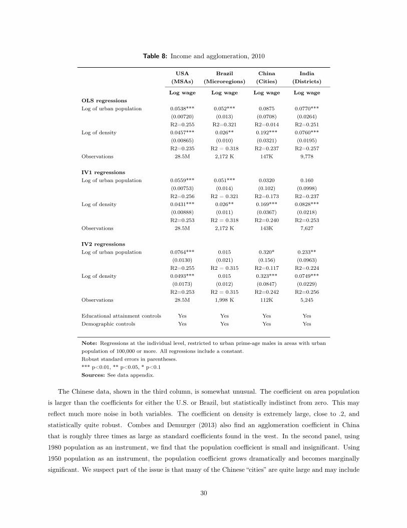
Table 8: Income and agglomeration, 2010
USA Brazil China India(MSAs) (Microregions) (Cities) (Districts)
Log wage Log wage Log wage Log wageOLS regressionsLog of urban population 0.0538*** 0.052*** 0.0875 0.0770***
(0.00720) (0.013) (0.0708) (0.0264)R2=0.255 R2=0.321 R2=0.014 R2=0.251
Log of density 0.0457*** 0.026** 0.192*** 0.0760***(0.00865) (0.010) (0.0321) (0.0195)R2=0.235 R2 = 0.318 R2=0.237 R2=0.257
Observations 28.5M 2,172 K 147K 9,778
IV1 regressionsLog of urban population 0.0559*** 0.051*** 0.0320 0.160
(0.00753) (0.014) (0.102) (0.0998)R2=0.256 R2 = 0.321 R2=0.173 R2=0.237
Log of density 0.0431*** 0.026** 0.169*** 0.0828***(0.00888) (0.011) (0.0367) (0.0218)R2=0.253 R2 = 0.318 R2=0.240 R2=0.253
Observations 28.5M 2,172 K 143K 7,627
IV2 regressionsLog of urban population 0.0764*** 0.015 0.320* 0.233**
(0.0130) (0.021) (0.156) (0.0963)R2=0.255 R2 = 0.315 R2=0.117 R2=0.224
Log of density 0.0493*** 0.015 0.323*** 0.0749***(0.0173) (0.012) (0.0847) (0.0229)
R2=0.253 R2 = 0.315 R2=0.242 R2=0.256Observations 28.5M 1,998 K 112K 5,245
Educational attainment controls Yes Yes Yes YesDemographic controls Yes Yes Yes Yes
Note: Regressions at the individual level, restricted to urban prime-age males in areas with urbanpopulation of 100,000 or more. All regressions include a constant.Robust standard errors in parentheses.*** p<0.01, ** p<0.05, * p<0.1Sources: See data appendix.
The Chinese data, shown in the third column, is somewhat unusual. The coefficient on area population
is larger than the coefficients for either the U.S. or Brazil, but statistically indistinct from zero. This may
reflect much more noise in both variables. The coefficient on density is extremely large, close to .2, and
statistically quite robust. Combes and Demurger (2013) also find an agglomeration coefficient in China
that is roughly three times as large as standard coefficients found in the west. In the second panel, using
1980 population as an instrument, we find that the population coefficient is small and insignificant. Using
1950 population as an instrument, the population coefficient grows dramatically and becomes marginally
significant. We suspect part of the issue is that many of the Chinese “cities” are quite large and may include
30
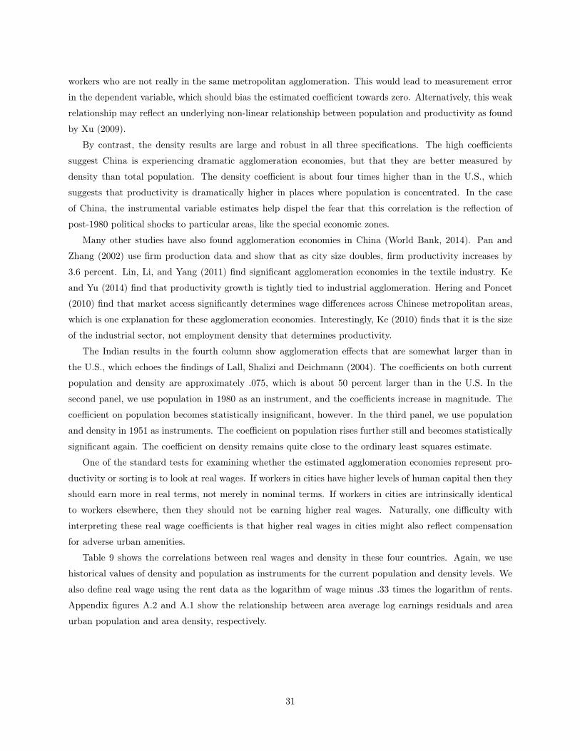
workers who are not really in the same metropolitan agglomeration. This would lead to measurement error
in the dependent variable, which should bias the estimated coefficient towards zero. Alternatively, this weak
relationship may reflect an underlying non-linear relationship between population and productivity as found
by Xu (2009).
By contrast, the density results are large and robust in all three specifications. The high coefficients
suggest China is experiencing dramatic agglomeration economies, but that they are better measured by
density than total population. The density coefficient is about four times higher than in the U.S., which
suggests that productivity is dramatically higher in places where population is concentrated. In the case
of China, the instrumental variable estimates help dispel the fear that this correlation is the reflection of
post-1980 political shocks to particular areas, like the special economic zones.
Many other studies have also found agglomeration economies in China (World Bank, 2014). Pan and
Zhang (2002) use firm production data and show that as city size doubles, firm productivity increases by
3.6 percent. Lin, Li, and Yang (2011) find significant agglomeration economies in the textile industry. Ke
and Yu (2014) find that productivity growth is tightly tied to industrial agglomeration. Hering and Poncet
(2010) find that market access significantly determines wage differences across Chinese metropolitan areas,
which is one explanation for these agglomeration economies. Interestingly, Ke (2010) finds that it is the size
of the industrial sector, not employment density that determines productivity.
The Indian results in the fourth column show agglomeration effects that are somewhat larger than in
the U.S., which echoes the findings of Lall, Shalizi and Deichmann (2004). The coefficients on both current
population and density are approximately .075, which is about 50 percent larger than in the U.S. In the
second panel, we use population in 1980 as an instrument, and the coefficients increase in magnitude. The
coefficient on population becomes statistically insignificant, however. In the third panel, we use population
and density in 1951 as instruments. The coefficient on population rises further still and becomes statistically
significant again. The coefficient on density remains quite close to the ordinary least squares estimate.
One of the standard tests for examining whether the estimated agglomeration economies represent pro-
ductivity or sorting is to look at real wages. If workers in cities have higher levels of human capital then they
should earn more in real terms, not merely in nominal terms. If workers in cities are intrinsically identical
to workers elsewhere, then they should not be earning higher real wages. Naturally, one difficulty with
interpreting these real wage coefficients is that higher real wages in cities might also reflect compensation
for adverse urban amenities.
Table 9 shows the correlations between real wages and density in these four countries. Again, we use
historical values of density and population as instruments for the current population and density levels. We
also define real wage using the rent data as the logarithm of wage minus .33 times the logarithm of rents.
Appendix figures A.2 and A.1 show the relationship between area average log earnings residuals and area
urban population and area density, respectively.
31
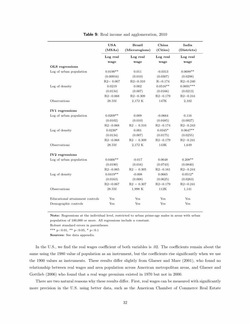
Table 9: Real income and agglomeration, 2010
USA Brazil China India(MSAs) (Microregions) (Cities) (Districts)
Log real Log real Log real Log realwage wage wage wage
OLS regressionsLog of urban population 0.0190** 0.011 -0.0313 0.0688**
(0.00916) (0.010) (0.0307) (0.0298)R2= 0.067 R2=0.310 R=0.174 R2=0.240
Log of density 0.0219 0.002 0.0516** 0.0691***(0.0134) (0.007) (0.0166) (0.0213)
R2=0.068 R2=0.309 R2=0.179 R2=0.244Observations 28.5M 2,172 K 147K 2,102
IV1 regressionsLog of urban population 0.0209** 0.009 -0.0664 0.116
(0.0102) (0.010) (0.0485) (0.0927)R2=0.068 R2 = 0.310 R2=0.174 R2=0.243
Log of density 0.0230* 0.001 0.0345* 0.0647**(0.0134) (0.007) (0.0175) (0.0255)
R2=0.068 R2 = 0.309 R2=0.179 R2=0.241Observations 28.5M 2,172 K 143K 1,649
IV2 regressionsLog of urban population 0.0466** -0.017 0.0648 0.208**
(0.0190) (0.016) (0.0743) (0.0840)R2=0.065 R2 = 0.305 R2=0.161 R2=0.244
Log of density 0.0419** -0.008 0.0665 0.0512*(0.0163) (0.008) (0.0625) (0.0263)
R2=0.067 R2 = 0.307 R2=0.179 R2=0.241Observations 28.5M 1,998 K 112K 1,141
Educational attainment controls Yes Yes Yes YesDemographic controls Yes Yes Yes Yes
Note: Regressions at the individual level, restricted to urban prime-age males in areas with urbanpopulation of 100,000 or more. All regressions include a constant.Robust standard errors in parentheses.*** p<0.01, ** p<0.05, * p<0.1Sources: See data appendix.
In the U.S., we find the real wages coefficient of both variables is .02. The coefficients remain about the
same using the 1980 value of population as an instrument, but the coefficients rise significantly when we use
the 1900 values as instruments. These results differ slightly from Glaeser and Mare (2001), who found no
relationship between real wages and area population across American metropolitan areas, and Glaeser and
Gottlieb (2006) who found that a real wage premium existed in 1970 but not in 2000.
There are two natural reasons why these results differ. First, real wages can be measured with significantly
more precision in the U.S. using better data, such as the American Chamber of Commerce Real Estate
32
Association price indices. We did not do that here to ensure comparability with other countries. Second,
in those papers the regressions are weighted at the metropolitan area level, while here they are weighted at
the person level. Nevertheless, these results still suggest that the majority of the agglomeration effect in
the U.S. does not reflect sorting, since these coefficients are so much smaller than the coefficient on nominal
wages.
For Brazil, there is no evidence suggesting that there is a real-wage premium in bigger cities. All of the
coefficients are quite close to zero. This fact pushes against the view that the Brazilian urban wage premium
reflects omitted human capital characteristics.
In the third column, we show results for China. In previous work, Au and Henderson (2006a) found that
real incomes initially rise with city size in China and then decline in the largest cities. This is consistent
with the fact that we find in our linear specification a negative but statistically insignificant coefficient.
The density coefficient remains positive, but is much smaller than the density coefficient for nominal wages.
Unless amenities are much higher in denser areas in China, this suggests that most of the nominal-wage
premium received in denser Chinese areas does not reflect sorting of higher-ability people into those areas.
Finally, the Indian regressions in the last column show that the nominal-wage premium in India that is
associated with both density and population is essentially the same as the real-wage premium. The results
are comparable when we use the recent lag of population as an instrument and implausibly large when we
use the long lag of population as an instrument. In a sense, these results are unsurprising given that we
have already seen that rents and incomes are essentially unrelated across Indian cities and real wages, in our
regressions, are just nominal wages corrected for rents.
There are two plausible interpretations for this strong relationship between real wages and agglomeration
in India. First, it is possible that Indian urbanites do, in fact, have much higher human capital levels than
rural Indians. Migration rates are low, and education quality may be quite different between urban and rural
areas. Second, it is also possible that our rent measures are so bad that these regressions have basically no
information value.
We supplement these real-wage regressions with Appendix Figure A.3, which shows the connection be-
tween happiness and area population for the U.S., China and India. In the U.S., there is essentially no
correlation between area population and happiness, which corroborates the finding that there is little real-
wage premium in larger cities. The correlation for China is also statistically indistinct from zero. This finding
is corroborated by a small literature on happiness and urbanization within China. Knight and Gunatilaka
(2010b, 2010a) find that wealthier urbanites in China are actually less happy than rural dwellers, perhaps
suggesting that migrants are forgoing current well-being for future economic prosperity. Cheng, Wang and
Smyth (2014) find that second generation rural-urban migrants are less satisfied than the first generation
of migrants. Within India, however, there is a large correlation between self-reported happiness and area
population, which is consistent with the positive real-wage premium associated with area size in that country.
Appendix Table A.1 repeats these regressions where rent, rather than income or real income, is the
dependent variable. Rents rise significantly with population and density in Brazil, China and the U.S. Rents
are unrelated to population and density in India. Again, this highlights the difficulties of using rental data
33
in the developing world.
Taking this evidence at face value, it appears that agglomeration economies are stronger in India and
China than in Brazil or the U.S. There is some possibility that the robust agglomeration effects observed
in India are driven by sorting. Still, there is every reason to believe that the literature that explains and
examines agglomeration economies in the developed world will continue to be relevant in the developing
world.
Human Capital Externalities
One prominent theory of agglomeration economies is that knowledge and ideas spread across space. The
theory also predicts human capital externalities: people who work and live in better educated areas will
themselves become more productive because they will accumulate more human capital. Rauch (1993) and
Moretti (2004) are two key contributors to this literature, which consistently estimates a significant relation-
ship between area-level education and earnings, holding individual-level education constant.
Naturally, the same two problems that bedevil agglomeration regressions also trouble human capital ex-
ternality regressions. It is possible that some omitted productivity variable both disproportionately attracts
skilled people to an area and increases wages. It is even more likely that places with higher levels of educa-
tion also have people with higher levels of unobserved human capital. The issue of sorting on unobservable
human capital is even more severe than in the case of agglomeration economies, because the key indepen-
dent variable is the level of observable human capital, not the level of density. It seems quite likely that
unobservable and observable human capital move together.
Acemoglu and Angrist (2001) attempt to address the omitted variables problems by using the variation
in compulsory education rules by state to estimate human capital spillovers. They find no spillovers with
this approach, but their source of variation is not ideal for estimating standard human capital spillover
models. For example, Glaeser (1999) provides a model of learning from neighbors in which raising the top
of the human capital distribution will generate spillovers, but raising the bottom of the distribution (which
is essentially the effect of raising the minimum school-leaving age) will not. Moretti (2004) tries different
instrumental variable approaches and finds consistent support for the existence of such spillovers.
Again, we have no magic bullet for addressing the sorting and omitted variables problems. Primarily
for robustness, we will show two instrumental variable regressions as well as the ordinary least squares
regressions. We instrument using a recent but lagged value of the local education variable, typically from1980.
We also follow Moretti (2004) and use the demographic structure of the city as an instrument for education
in the second panel of the table. Specifically, we predict age-group shares of the area population based on the
population shares of each group in the area in 1980. We then attribute to each age group the education level
that is typical for that age group in 2010. Essentially, our instrument is the predicted instrument for the
area if it had kept its age structure from 1980 and if everybody had his or her age group’s average education.
In all cases, our education measure will be the share of the population with a post-secondary degree, which
has the advantage of being readily available and relatively comparable across areas.
34
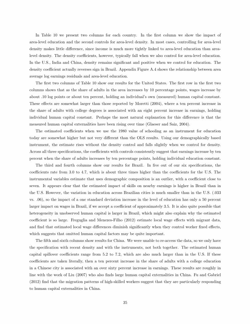
In Table 10 we present two columns for each country. In the first column we show the impact of
area-level education and the second controls for area-level density. In most cases, controlling for area-level
density makes little difference, since income is much more tightly linked to area-level education than area-
level density. The density coefficients, however, typically fall when we also control for area-level education.
In the U.S., India and China, density remains significant and positive when we control for education. The
density coefficient actually reverses sign in Brazil. Appendix Figure A.4 shows the relationship between area
average log earnings residuals and area-level education.
The first two columns of Table 10 show our results for the United States. The first row in the first two
columns shows that as the share of adults in the area increases by 10 percentage points, wages increase by
about .10 log points or about ten percent, holding an individual’s own (measured) human capital constant.
These effects are somewhat larger than those reported by Moretti (2004), where a ten percent increase in
the share of adults with college degrees is associated with an eight percent increase in earnings, holding
individual human capital constant. Perhaps the most natural explanation for this difference is that the
measured human capital externalities have been rising over time (Glaeser and Saiz, 2004).
The estimated coefficients when we use the 1980 value of schooling as an instrument for education
today are somewhat higher but not very different than the OLS results. Using our demographically based
instrument, the estimate rises without the density control and falls slightly when we control for density.
Across all three specifications, the coefficients with controls consistently suggest that earnings increase by ten
percent when the share of adults increases by ten percentage points, holding individual education constant.
The third and fourth columns show our results for Brazil. In five out of our six specifications, the
coefficients rate from 3.0 to 4.7, which is about three times higher than the coefficients for the U.S. The
instrumental variables estimate that uses demographic composition is an outlier, with a coefficient close to
seven. It appears clear that the estimated impact of skills on nearby earnings is higher in Brazil than in
the U.S. However, the variation in education across Brazilian cities is much smaller than in the U.S. (.033
vs. .06), so the impact of a one standard deviation increase in the level of education has only a 50 percent
larger impact on wages in Brazil, if we accept a coefficient of approximately 3.5. It is also quite possible that
heterogeneity in unobserved human capital is larger in Brazil, which might also explain why the estimated
coefficient is so large. Freguglia and Menezes-Filho (2012) estimate local wage effects with migrant data,
and find that estimated local wage differences diminish significantly when they control worker fixed effects,
which suggests that omitted human capital factors may be quite important.
The fifth and sixth columns show results for China. We were unable to re-access the data, so we only have
the specification with recent density and with the instruments, not both together. The estimated human
capital spillover coefficients range from 5.2 to 7.2, which are also much larger than in the U.S. If these
coefficients are taken literally, then a ten percent increase in the share of adults with a college education
in a Chinese city is associated with an over sixty percent increase in earnings. These results are roughly in
line with the work of Liu (2007) who also finds large human capital externalities in China. Fu and Gabriel
(2012) find that the migration patterns of high-skilled workers suggest that they are particularly responding
to human capital externalities in China.
35
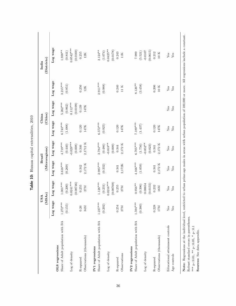
Tabl
e10
:H
uman
capi
tale
xter
nalit
ies,
2010
USA
Bra
zil
Chin
aIn
dia
(MSA
s)(M
icro
regi
ons)
(Citie
s)(D
istr
icts
)
Log
wag
eLog
wag
eLog
wag
eLog
wag
eLog
wag
eLog
wag
eLog
wag
eLog
wag
eO
LS
regr
essi
ons
Shar
eof
Adu
ltpo
pula
tion
with
BA
1.27
2***
1.00
1***
3.61
6***
4.71
9***
6.74
3***
5.26
2***
3.21
5***
1.93
8**
(0.1
55)
(0.2
00)
(0.2
69)
(0.4
40)
(1.0
88)
(0.8
62)
(0.8
51)
(0.8
41)
Log
ofde
nsity
0.02
41**
*-0
.029
***
0.11
2***
0.05
42**
*(0
.007
46)
(0.0
08)
(0.0
199)
(0.0
169)
R-s
quar
ed0.
260.
255
0.34
20.
346
0.12
00.
139
0.25
60.
255
Obs
erva
tion
s(t
hous
ands
)34
M27
M2,
172
K2,
1712
K14
7K14
7K12
K12
K
IV1
regr
essi
ons
Shar
eof
Adu
ltpo
pula
tion
with
BA
1.23
7***
1.12
6***
2.98
5***
3.78
4***
6.57
2***
2.91
1***
2.12
4**
(0.2
02)
(0.2
31)
(0.3
32)
(0.4
86)
(0.9
25)
(0.9
88)
(1.0
74)
Log
ofde
nsity
0.02
16**
*-0
.018
**0.
0425
**(0
.007
69)
(0.0
09)
(0.0
178)
R-s
quar
ed0.
254
0.25
50.
341
0.34
40.
120
0.24
00.
243
Obs
erva
tion
s27
M27
M2,
172K
2,17
2K
147K
11K
11K
IV2
regr
essi
ons
Shar
eof
Adu
ltpo
pula
tion
with
BA
1.59
4***
0.95
6**
4.16
6***
6.70
5***
7.18
9***
8.12
6**
7.98
9(0
.380
)(0
.396
)(1
.059
)(1
.756
)(1
.437
)(3
.458
)(5
.521
)Log
ofde
nsity
0.00
654
-0.0
52**
-0.0
107
(0.0
155)
(0.0
23)
(0.0
615)
R-s
quar
ed0.
228
0.23
20.
341
0.34
10.
120
0.20
60.
212
Obs
erva
tion
s(t
hous
ands
)17
M16
M2,
172
K2,
172
K14
7K10
K10
K
Edu
cation
alat
tain
men
tco
ntro
lsYes
Yes
Yes
Yes
Yes
Yes
Yes
Yes
Age
cont
rols
Yes
Yes
Yes
Yes
Yes
Yes
Yes
Yes
Not
e:R
egre
ssio
nsat
the
indi
vidu
alle
vel,
rest
rict
edto
urba
npr
ime-
age
mal
esin
area
sw
ith
urba
npo
pula
tion
of10
0,00
0or
mor
e.A
llre
gres
sion
sin
clud
ea
cons
tant
.R
obus
tst
anda
rder
rors
inpa
rent
hese
s.**
*p<
0.01
,**
p<0.
05,*
p<0.
1Sou
rces
:Se
eda
taap
pend
ix.
36
The variation in education rates across cites is also smaller in China than in the U.S., but larger than
in Brazil. The impact of one standard deviation increase in area level education in China is associated with
a 20 percent increase in earnings if we use the most conservative estimate. The comparable figure with the
U.S. is a six percent increase in earnings.
The same pattern reappears for India in the seventh and eighth columns. With the exception of the
demographically constructed instrumental variable regression, the coefficients range from 1.9 to 3.2. These
are higher than in the U.S., but lower than either Brazil or China. A one standard deviation increase in area
level education (.033) in India is associated with an approximately seven percent increase in earnings, if we
accept a coefficient of 2.1, which is only marginally higher than in the U.S. A ten percentage point increase
in the share of adults with college degrees is associated with a 21 percent increase in earnings, which is more
than double the U.S. figure.
All three developing countries show a similar pattern. Education levels vary less across space than in
the U.S. The estimated effect of area level education on wages is much higher than in the U.S. One class
of explanations for these differences assumes that these human capital coefficients are largely spurious. A
second class of explanations assumes that they are real.
For example, if we believe that the coefficients are spurious because of sorting on unobservables, then
the correlation between unobervables and area level education is likely to be much higher in countries with
less variation in education. If the regression was univariate, then the bias created by unobservable human
capital would equal Cov(Log(Wage),UnobservableHumanCapital)V ar(ObservedHumanCapital) . If variance of observed human capital is small,
then the bias blows up proportionately.
A second type of explanation assumes that the effect is real. In that case, the high coefficients might
mean that local human capital is more valuable in developing world cities than elsewhere. Local human
capital might be more important in places that have lower levels of development and less such capital.
We will not try to resolve these issues here, but we believe that these extremely high measured levels of
human capital externalities especially in Brazil and China suggest that this is an important topic for future
research. If these results reflect a true human capital spillover, then developing world cities success really
depends on education. We now ask whether education also seems to have dynamic effects on cities in the
developing world.
Urban Growth and Human Capital
While Gibrat’s Law tells us that urban growth is not correlated with initial population levels, a long literature
documents the connection between skills and subsequent growth within the United States and internationally.
Glaeser, Scheinkman and Shleifer (1995) documented the correlation between the share of adults with college
degrees and population growth between 1960 and 1990 within the U.S. Subsequent work (Glaeser and Saiz,
2004; Shapiro, 2006) has shown that this correlation persists for more recent periods, and that skills also
predict the growth of income at the local level within the U.S. Simon and Nardinelli (2002) show that 19th
37
century skills predict growth over the next century within the U.S. Using a sample of over 1,500 regions
from 83 countries, Gennaioli, La Porta, Lopez de Silanes and Shleifer (2014) also find a connection between
initial levels of human capital and regional growth.
Several hypotheses have been advanced to explain the skills-growth connection. Glaeser, Scheinkman and
Shleifer (1995) originally suggested that skills sped growth by encouraging the increase of local productivity.
Glaeser and Saiz (2004) find that measured human capital externalities have grown stronger over time.
Alternatively, skills may have also been correlated with amenities that have gotten more desirable, or with
good government. Our goal is not to distinguish between these hypotheses, but rather to look at whether
the skills growth connection also exists in Brazil, China and India.
Table 11 shows our results when we regress population and income change between 1980 and 2010 on
the share of adults with tertiary education in 1980. We present four regressions for each country: one with
just education for both income and population growth and one with added controls, which is our preferred
specification. The added controls include initial income and population, as well as climate controls. Unlike
other regressions in the paper, Table 11 uses total rather than urban populations.3
The first regressions in the upper panel show results for the U.S. A ten percent increase in the share of
the population with a college degree in 1980 is associated with a 17 percent increase in population between
1980 and 2010. This effect is statistically and economically meaningful and it is shown in Figure 5. The
second regression shows that the estimated coefficient increases to 2.16 when we control for initial income
and population. The t-statistic is over six, which indicates the strength and robustness of the connection
between skills and area population growth over this time period.
The lower two regressions show the results for income growth within the U.S. The coefficient on initial
schooling is .5. With the controls, the coefficient rises to .9, which is both statistically significant and
economically meaningful. Ten percentage points more college graduates in 1980 is associated with about
nine percent higher income growth between 1980 and 2010. Initial income controls are particularly important
because income levels typically mean revert, and higher education area in 1980 also had higher income levels.
Controlling for initial income corrects for the mean reversion of income.
Our next four regressions show the results for Brazil. The population growth pattern is similar to the
U.S., in that the correlation with initial skills becomes stronger when we control for other variables. A ten
percentage point increase in the share of the population with college degrees in 1980 is associated with about
49 percent more population growth between 1980 and 2010. The coefficient increases to over five when we
control for other variables.
3In 1980 Brazil, China and India had much lower urbanization rates than the U.S., and urbanization rates differed signifi-cantly across areas. Regions with lower urbanization tend to have lower formal education levels (Young, 2013). If city growthin low-urbanization regions is disproportionally driven by own-region rural-urban migration, there can be a spurious connectionbetween initial low area education levels and faster growth in urban population. Looking at total populations mitigates thisconcern, and allows us to better approximate the growth effect of human capital across areas.
38
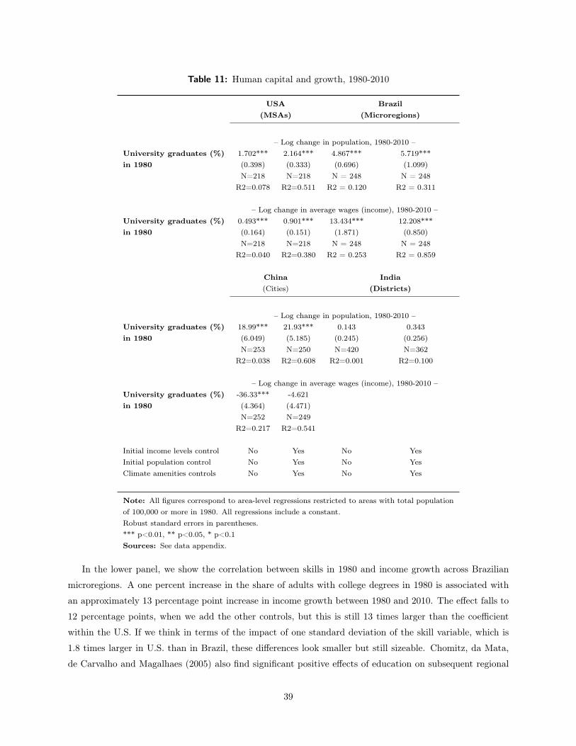
Table 11: Human capital and growth, 1980-2010
USA Brazil(MSAs) (Microregions)
– Log change in population, 1980-2010 –University graduates (%) 1.702*** 2.164*** 4.867*** 5.719***in 1980 (0.398) (0.333) (0.696) (1.099)
N=218 N=218 N = 248 N = 248R2=0.078 R2=0.511 R2 = 0.120 R2 = 0.311
– Log change in average wages (income), 1980-2010 –University graduates (%) 0.493*** 0.901*** 13.434*** 12.208***in 1980 (0.164) (0.151) (1.871) (0.850)
N=218 N=218 N = 248 N = 248R2=0.040 R2=0.380 R2 = 0.253 R2 = 0.859
China India(Cities) (Districts)
– Log change in population, 1980-2010 –University graduates (%) 18.99*** 21.93*** 0.143 0.343in 1980 (6.049) (5.185) (0.245) (0.256)
N=253 N=250 N=420 N=362R2=0.038 R2=0.608 R2=0.001 R2=0.100
– Log change in average wages (income), 1980-2010 –University graduates (%) -36.33*** -4.621in 1980 (4.364) (4.471)
N=252 N=249R2=0.217 R2=0.541
Initial income levels control No Yes No YesInitial population control No Yes No YesClimate amenities controls No Yes No Yes
Note: All figures correspond to area-level regressions restricted to areas with total populationof 100,000 or more in 1980. All regressions include a constant.Robust standard errors in parentheses.*** p<0.01, ** p<0.05, * p<0.1Sources: See data appendix.
In the lower panel, we show the correlation between skills in 1980 and income growth across Brazilian
microregions. A one percent increase in the share of adults with college degrees in 1980 is associated with
an approximately 13 percentage point increase in income growth between 1980 and 2010. The effect falls to
12 percentage points, when we add the other controls, but this is still 13 times larger than the coefficient
within the U.S. If we think in terms of the impact of one standard deviation of the skill variable, which is
1.8 times larger in U.S. than in Brazil, these differences look smaller but still sizeable. Chomitz, da Mata,
de Carvalho and Magalhaes (2005) also find significant positive effects of education on subsequent regional
39
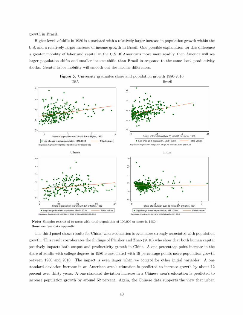
growth in Brazil.
Higher levels of skills in 1980 is associated with a relatively larger increase in population growth within the
U.S. and a relatively larger increase of income growth in Brazil. One possible explanation for this difference
is greater mobility of labor and capital in the U.S. If Americans move more readily, then America will see
larger population shifts and smaller income shifts than Brazil in response to the same local productivity
shocks. Greater labor mobility will smooth out the income differences.
Figure 5: University graduates share and population growth 1980-2010USA Brazil
−.5
0.5
11
.5
0 .05 .1 .15Share of Population Over 25 with BA or Higher, 1980.
Log change in population, 1980−2010 Fitted values
Regression: PopGrowth= 0.31( 0.03)+ 4.87( 0.70) Share BA 1980. (R2= 0.12)
China India
Note: Samples restricted to areas with total population of 100,000 or more in 1980.Sources: See data appendix.
The third panel shows results for China, where education is even more strongly associated with population
growth. This result corroborates the findings of Fleisher and Zhao (2010) who show that both human capital
positively impacts both output and productivity growth in China. A one percentage point increase in the
share of adults with college degrees in 1980 is associated with 19 percentage points more population growth
between 1980 and 2010. The impact is even larger when we control for other initial variables. A one
standard deviation increase in an American area’s education is predicted to increase growth by about 12
percent over thirty years. A one standard deviation increase in a Chinese area’s education is predicted to
increase population growth by around 52 percent. Again, the Chinese data supports the view that urban
40
success is quite closely correlated with initial skills in the developing world.
The lower two regressions for China show a somewhat more mixed picture for income growth. Without
other controls, there is a negative correlation between initial education and income growth across Chinese
cities. With initial controls, the negative effect is much smaller and statistically insignificant.
Perhaps the most natural explanation for the Chinese pattern is that cities were far from an equilibrium
in 1980, because of profound restrictions on mobility in China. In a world in which migration is initially
forbidden and where skilled cities are more productive than unskilled cities, allowing free migration will
cause the population of skilled cities to soar and the incomes of skilled cities to decline. As population flows
rapidly into skilled cities after liberalization, wages in those areas will consequently decline. Despite the large
population moves, skilled Chinese cities have also seen income increases which suggests that those areas are
also seeing some productivity growth, although not enough to overwhelm the impact of migration.
The final panel shows results for India, where we only have population growth. Without other controls,
the impact of initial skills on population growth is weakly positive. With controls, the estimated coefficient
becomes larger but still much smaller than in the other countries and statistically insignificant. As in the
human capital externality regressions, the link between education and urban success seems weaker in India
than in the other developing countries.
Overall, however, this section supported the view that agglomeration and human capital are strong
determinants of urban success in the developing world. Area size is more strongly correlated with income in
China and India than in the U.S. and Brazil. Area education has a much stronger connection with income
in the developing world than in the U.S. Area education also strongly predicts population growth in Brazil
and China, if not in India, as well as income growth in Brazil. We conclude from these facts that the long
literatures on agglomeration economies, human capital externalities and growth and skills in the developed
world are likely to be relevant in the developing world as well.
VI. Conclusion
In this paper, we performed three types of comparisons. First, we compared the basic patterns of urban
size and growth in the four large countries. Second, we looked at whether U.S. based tests of the Rosen-
Roback framework yield similar results in Brazil, China and India. Third, we look at whether agglomeration
economies and human capital externalities seen to operate similarly in the four countries.
The Zipf’s law distributions were not identical across the four countries. Most notably, India and China
had too few ultra-large cities relative to what Zipf’s law would predict. The natural explanation for this fact
is that congestion disamenities would be too severe for cities of 50 or 100 million people. From 1980 to 2010,
Gibrat’s law seems to hold for the U.S. and Brazil, but not for India and China. Among Indian districts,
growth was larger in initially larger areas between 1981 and 1991, but smaller over the whole 1981-2011
period.
The most basic Rosen-Roback fact is the strong correlation between income and housing costs across
metropolitan areas in the U.S., although even the U.S. quantitative relationship is too small relative to the
41
predictions of theory. The relationship between income and rents is similar in Brazil, China and the U.S.
India, surprisingly, shows no spatial relationship between income and rents, which may reflect data issues or
chaotic rental markets. In the U.S., real wages decline in places with better climates. This is not true in any
of the other countries. There is little relationship between income and happiness across U.S. areas, which is
also compatible with the spatial equilibrium. The relationship is stronger, though imprecisely measured, in
China and India.
All together, the spatial equilibrium framework fits the data far more poorly in India than in the U.S.
and Brazil. China’s data is more consistent with the spatial equilibrium predictions than India, but not
as much as Brazil. One explanation for this failure is that unobserved human capital heterogeneity is far
more severe in India and China than in the more urbanized, richer countries. A second explanation is that
mobility is limited, either by rules, such as China’s Hukuo system, or by strong place-based preferences such
as those related to cast-based social networks in India.
While the spatial equilibrium framework fares much more poorly in the less-urbanized developing world
data, the urban productivity and growth relationships are far stronger in those countries. For example, the
coefficient when individual income is regressed on area density is around .05 in the U.S. and .03 in Brazil.
The coefficient rises to .2 for China and .08 for India. We cannot rule out that this relationship is driven by
unobserved human capital, but we can say that the within–country link between density and prosperity in
these places does seem remarkably strong.
Similarly, the connection between human capital and area success is also stronger in the developing world
countries. For example, the core human capital externality coefficient, when log of earnings is regressed on
the share of adults with a college degree or more, is approximately one in the U.S., controlling for individual
human capital characteristics. In Brazil, China and India, the same coefficient ranges from two to five. This
enormously strong link between area skills and area earnings, controlling for individual skill, may be driven
by omitted human capital but it is certainly worth of more research.
As in the U.S., skill also predicts urban growth in Brazil and China. In our preferred specification, a
one percentage point increase in the share of college graduates in 1980 is associated with a seven percentage
point increase in population between 1980 and 2010 in Brazil and a 22 percent point increase in population
in China. The effect is much weaker in India. Human capital is also strongly associated with income growth
in Brazil.
Taken together, these results suggest that the U.S. facts do matter for the developing world, but they
matter more in some places than others, and they matter more in some areas of study than others. Across
the board, Brazil is the most like the U.S. and China is second most like the U.S. India is different, probably
because of its extremely low mobility rates and much lower income levels.
Our interpretation of these results is that skills and agglomeration impact productivity globally in rich
and poor countries alike, but that a spatial equilibrium evolves over time. In the poorest places, social
ties to home communities are strong. Historically, they provided safety and sustenance. As nations evolve
into wealthy market economies with more homogenous human capital, a spatial equilibrium may eventually
appear in countries like India, where it still has not emerged.
42
Developing world urbanization is among the most important social phenomena globally, but we know
much more about developed world urbanization. This paper has shown that some, but not all of that
developed world knowledge can be exported to Brazil, China and India. The facts from the west must now
be supplemented with a robust research agenda on developing world cities.
References
Acemoglu, D., Angrist, J., 2001. How Large are Human-Capital Externalities ? Evidence from Compulsory
Schooling Laws. NBER Macroeconomics Annual 2000, Volume 15 15 (January), 9–74.
Albouy, D., 2015. What Are Cities Worth? Land Rents, Local Productivity, and the Total Value of Amenities.
Alonso, W., 1964. Location and Land Use. Harvard University Press, Cambridge, Mass, Cambridge, MA.
Anderson, G., Ge, Y., 2005. The size distribution of Chinese cities. Regional Science and Urban Economics
35 (6), 756–776.
Arriaga, E., 1968. Components of city growth in selected Latin American countries. The Milbank Memorial
Fund Quarterly 46 (2), 237–252.
Au, C.-C., Henderson, J. V., 2006a. Are Chinese Cities Too Small? Review of Economic Studies 73, 549–576.
Au, C. C., Henderson, J. V., 2006b. How migration restrictions limit agglomeration and productivity in
China. Journal of Development Economics 80, 350–388.
Azzoni, C. R., Menezes-Filho, N., Silveira-Neto, R., 2000. Geography and income convergence among Brazil-
ian states (May), 30.
Azzoni, C. R., Servo, L. M. S., 2002. Education, cost of living and regional wage inequality in Brazil. Papers
in Regional Science 81 (2), 157–175.
Bell, M., Muhidin, S., 2009. Cross-National Comparisons of Internal Migration.
Champernowne, D., 1953. A Model of Income Distribution. The Economic Journal 63 (250), 318–351.
Chan, K., 2007. Misconceptions and Complexities in the Study of China’s Cities: Definitions, Statistics, and
Implications. Eurasian Geography and Economics 48 (4), 383–412.
Cheng, Z., Wang, H., Smyth, R., 2014. Happiness and job satisfaction in urban China: A comparative study
of two generations of migrants and urban locals. Urban Studies 51 (10), 2160–2184.
Chomitz, K. M., da Mata, D., de Carvalho, A. Y., Magalhães, J. C., 2005. Spatial dynamics of labor markets
in Brazil. Policy Research Working Paper (3752).
Combes, P.-P., Démurger, S., Li, S., 2013. Urbanisation and Migration Externalities in China, 37.
43
Combes, P.-P., Duranton, G., Gobillon, L., Roux, S., 2010. Estimating agglomeration economies with history,
geology, and worker effects. In: The economics of agglomeration. Vol. I. pp. 15–65.
Combes, P.-p., Gobillon, L., 2014. The Empirics of Agglomeration Economies.
Corbi, R. B., Menezes-Filho, N. A., 2006. Os determinantes empíricos da felicidade no Brasil. Revista de
Economia Política 26 (4), 518–536.
Diamond, R., 2015. The Determinants and Welfare Implications of US Workers’ Diverging Location Choices
by Skill: 1980-2000.
Durand, J. D., Pelaez, C., 1965. Patterns of Urbanization in Latin America. In: Proceedings of the Sixtieth
Anniversary Conference of the Milbank Memorial Fund. Part 2: Components of Population Change in
Latin America. Vol. 43. The Milbank Memorial Fund Quarterly, pp. 166–196.
Feler, L., Henderson, J. V., 2011. Exclusionary policies in urban development: Under-servicing migrant
households in Brazilian cities. Journal of Urban Economics 69 (3), 253–272.
Fiess, N. M., Verner, D., 2003. Migration and human capital in Brazil during the 1990s. Tech. Rep. 3093.
Fleisher, B., Li, H., Zhao, M. Q., 2010. Human capital, economic growth, and regional inequality in China.
Journal of Development Economics 92 (2), 215–231.
Fontes, G. G., Simoes, R. F., De Oliveira, A. M., Hermeto, C., 2009. Urban Attributes and Wage Disparities
in Brazil: A Multilevel Hierarchical Model. Regional Studies 44 (5), 596–607.
Freguglia, R. S., Menezes-Filho, N. A., 2012. Inter-regional wage differentials with individual heterogeneity:
evidence from Brazil. The Annals of Regional Science 49 (1), 17–34.
Fu, Y., Gabriel, S. A., 2012. Labor migration, human capital agglomeration and regional development in
China. Regional Science and Urban Economics 42 (3), 473–484.
Gabaix, X., 1999. Zipf’s Law for Cities: An Explanation. The Quarterly Journal of Economics (August),
739–767.
Gabaix, X., Ibragimov, R., 2011. Rank-1/2: A Simple Way to Improve the OLS Estimation of Tail Exponents.
Journal of Business & Economic Statistics 29 (1), 24–39.
Gennaioli, N., La Porta, R., Lopez De Silanes, F., Shleifer, A., 2014. Growth in regions. Journal of Economic
Growth 19, 259–309.
Glaeser, E., Gottlieb, J. D., 2006. Urban resurgence and the consumer city. Urban Studies 43 (8), 1275–1299.
Glaeser, E. L., 1999. Learning in cities. Journal of urban Economics (46), 254–277.
Glaeser, E. L., 2008. Cities, Agglomeration and Spatial Equilibrium. Oxford University Press, New York.
44
Glaeser, E. L., Gottlieb, J. D., dec 2009. The Wealth of Cities: Agglomeration Economies and Spatial
Equilibrium in the United States. Journal of Economic Literature 47 (4), 983–1028.
Glaeser, E. L., Gottlieb, J. D., Ziv, O., 2014a. Unhappy Cities.
Glaeser, E. L., Maré, D. C., 2001. Cities and Skills. Journal of Labor Economics 19 (2), 316–342.
Glaeser, E. L., Ponzetto, G. A. M., Tobio, K., 2014b. Cities, Skills and Regional Change. Regional Studies
48 (1), 7–43.
Glaeser, E. L., Scheinkman, J. A., Shleifer, A., aug 1995. Economic growth in a cross-section of cities. Journal
of Monetary Economics 36 (1), 117–143.
Glaeser, E. L. E. L., Saiz, A., 2004. The Rise of the Skilled City. Brookings-Wharton Papers on Urban
Affairs 2004 (1), 47–105.
Hering, L., Poncet, S., 2010. Market Access and Individual Wages: Evidence From China. The Review of
Economics and Statistics 92 (1), pp. 145–159.
Holmes, T. J., Lee, S., 2010. Cities as Six-by-Six-Mile Squares Zipf’s Law? In: Glaeser, E. L. (Ed.),
Agglomeration Economics. No. February. The University of Chicago Press, pp. 105 – 131.
IBGE, 2002. Censo Demograafico 2000: Documentacao das Microdados da Amostra.
IPEA, 2012. 2012: Desenvolvimento Inclusivo Sustentável?
Jedwab, R., Vollrath, D., 2016. The Urban Mortality Transition and the Rise of Poor Mega Cities.
Ke, S., 2010. Agglomeration, productivity, and spatial spillovers across Chinese cities. Annals of Regional
Science 45 (1), 157–179.
Ke, S., Yu, Y., 2014. The pathways from industrial agglomeration to TFP growth - the experience of Chinese
cities for 2001-2010. Journal of the Asia Pacific Economy 19 (January), 310–332.
Knight, J., Gunatilaka, R., 2010a. Great Expectations? The Subjective Well-being of Rural-Urban Migrants
in China. World Development 38 (1), 113–124.
Knight, J., Gunatilaka, R., 2010b. The Rural-Urban Divide in China: Income but Not Happiness? Journal
of Development Studies 46 (October 2014), 506–534.
Kovak, B. K., 2013. Regional effects of trade reform: What is the correct measure of liberalization? American
Economic Review 103 (5), 1960–1976.
Lall, S. V., Shalizi, Z., Deichmann, U., apr 2004. Agglomeration economies and productivity in Indian
industry. Journal of Development Economics 73 (2), 643–673.
Lin, H. L., Li, H. Y., Yang, C. H., 2011. Agglomeration and productivity: Firm-level evidence from China’s
textile industry. China Economic Review 22 (3), 313–329.
45
Liu, Y., Shen, J., 2014. Jobs or Amenities? Location Choices of Interprovincial Skilled Migrants in China,
2000-2005. Population, Space and Place 20 (7), 592–605.
Liu, Z. Q., 2007. The external returns to education: Evidence from Chinese cities. Journal of Urban Eco-
nomics 61 (3), 542–564.
Long, F., Guo, M., Zheng, S., 2009. Estimating the Willingness-to-Pay for Urban Housing in Chinese Cities.
Tsinghua Science & Technology 14 (3), 360–366.
Mclanahan, S., Adams, J., 1987. Parenthood and Psychological Well-Being. Annual review of sociology
13 (1987), 237–257.
Melo, P. C., Graham, D. J., Noland, R. B., 2009. A meta-analysis of estimates of urban agglomeration
economies. Regional Science and Urban Economics 39 (3), 332–342.
Moretti, E., aug 2004. Estimating the social return to higher education: evidence from longitudinal and
repeated cross-sectional data. Journal of Econometrics 121 (1-2), 175–212.
Morten, M., 2013. Temporary Migration and Endogenous Risk Sharing in Village India.
Mueller, V., 2005. Valuating Climate Amenities in Brazil Using a Hedonic Pricing Framework. Doctoral
dissertation, University of Maryland at College Park.
Munshi, K., Rosenzweig, M., 2009. Why is Mobility in India so Low ? Social Insurance, Inequality, and
Growth.
Muth, R., 1969. Cities and Housing. University of Chicago Press., Chicago and London.
OECD, 2012. Redefining "Urban" - A New Way to Measure Metropolitan Areas. OECD Publishing, Paris.
OECD, 2015. OECD Urban Policy Reviews: China 2015. OECD Publishing, Paris.
Pan, Z., Zhang, F., 2002. Urban Productivity in China. Urban Studies 39 (12), 2267–2281.
Rauch, J. E., 1993. Productivity Gains from Geographic Concentration of Human Capital: Evidence from
the Cities. Journal of Urban Economics 34, 380–400.
Reis, E. J., Pimental, M., Alvarenga, A. I., 2007. Areas Minimas Comparaaveis para os Periodos Intercensi-
tarios de 1872 a 2000.
Resende, M., 2004. Gibrat’s law and the growth of cities in Brazil: A panel data investigation. Urban Studies
41 (8), 1537–1549.
Roback, J., 1982. Wages, rents, and the quality of life. The Journal of Political Economy 90 (6), 1257–1278.
Rose, A. K., 2006. Cities and Countries. Journal of Money, Credit and Banking 38 (8), 2225–2245.
46
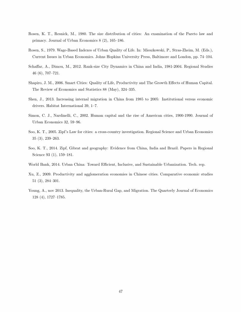
Rosen, K. T., Resnick, M., 1980. The size distribution of cities: An examination of the Pareto law and
primacy. Journal of Urban Economics 8 (2), 165–186.
Rosen, S., 1979. Wage-Based Indexes of Urban Quality of Life. In: Mieszkowski, P., Stras-Zheim, M. (Eds.),
Current Issues in Urban Economics. Johns Hopkins University Press, Baltimore and London, pp. 74–104.
Schaffar, A., Dimou, M., 2012. Rank-size City Dynamics in China and India, 1981-2004. Regional Studies
46 (6), 707–721.
Shapiro, J. M., 2006. Smart Cities: Quality of Life, Productivity and The Growth Effects of Human Capital.
The Review of Economics and Statistics 88 (May), 324–335.
Shen, J., 2013. Increasing internal migration in China from 1985 to 2005: Institutional versus economic
drivers. Habitat International 39, 1–7.
Simon, C. J., Nardinelli, C., 2002. Human capital and the rise of American cities, 1900-1990. Journal of
Urban Economics 32, 59–96.
Soo, K. T., 2005. Zipf’s Law for cities: a cross-country investigation. Regional Science and Urban Economics
35 (3), 239–263.
Soo, K. T., 2014. Zipf, Gibrat and geography: Evidence from China, India and Brazil. Papers in Regional
Science 93 (1), 159–181.
World Bank, 2014. Urban China: Toward Efficient, Inclusive, and Sustainable Urbanization. Tech. rep.
Xu, Z., 2009. Productivity and agglomeration economies in Chinese cities. Comparative economic studies
51 (3), 284–301.
Young, A., nov 2013. Inequality, the Urban-Rural Gap, and Migration. The Quarterly Journal of Economics
128 (4), 1727–1785.
47
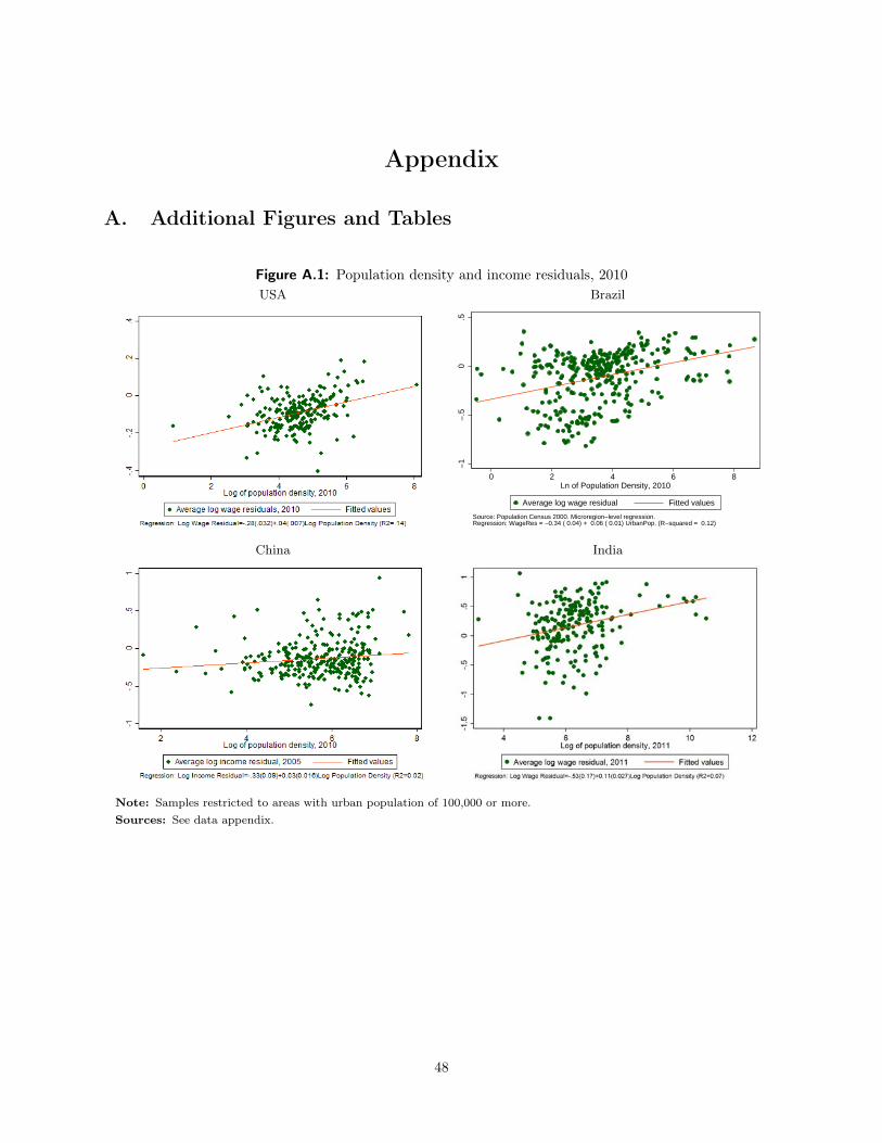
Appendix
A. Additional Figures and Tables
Figure A.1: Population density and income residuals, 2010USA Brazil
−1
−.5
0.5
0 2 4 6 8Ln of Population Density, 2010
Average log wage residual Fitted values
Source: Population Census 2000. Microregion−level regression.Regression: WageRes = −0.34 ( 0.04) + 0.06 ( 0.01) UrbanPop. (R−squared = 0.12)
China India
Note: Samples restricted to areas with urban population of 100,000 or more.Sources: See data appendix.
48
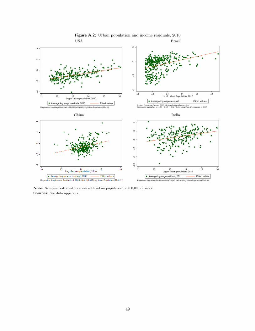
Figure A.2: Urban population and income residuals, 2010USA Brazil
−1
−.5
0.5
11 12 13 14 15 16Ln of Urban Population, 2010
Average log wage residual Fitted values
Source: Population Census 2000. Microregion−level regression.Regression: WageRes = −1.57 ( 0.18) + 0.12 ( 0.01) UrbanPop. (R−squared = 0.13)
China India
Note: Samples restricted to areas with urban population of 100,000 or more.Sources: See data appendix.
49
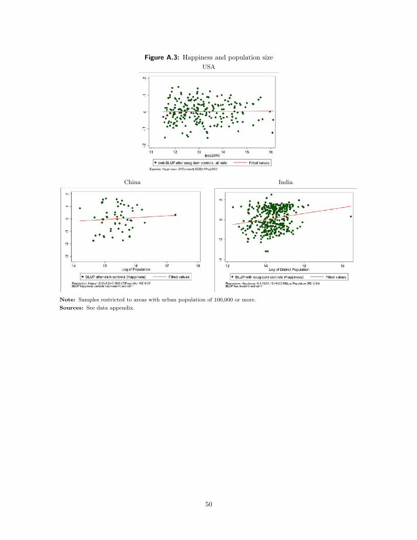
Figure A.3: Happiness and population sizeUSA
China India
Note: Samples restricted to areas with urban population of 100,000 or more.Sources: See data appendix.
50
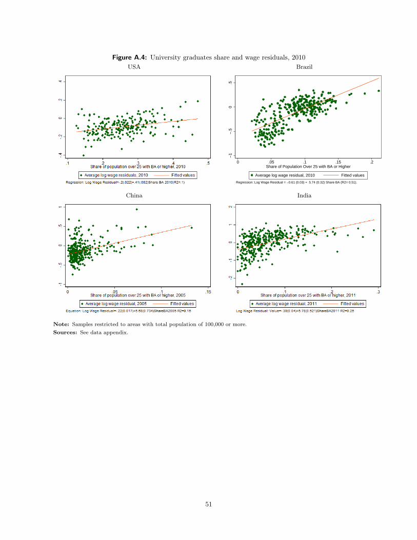
Figure A.4: University graduates share and wage residuals, 2010USA Brazil
−1
−.5
0.5
0 .05 .1 .15 .2Share of Population Over 25 with BA or Higher
Average log wage residual, 2010 Fitted values
Regression: Log Wage Residual = −0.61 (0.03) + 5.74 (0.32) Share BA (R2= 0.51).
China India
Note: Samples restricted to areas with total population of 100,000 or more.Sources: See data appendix.
51
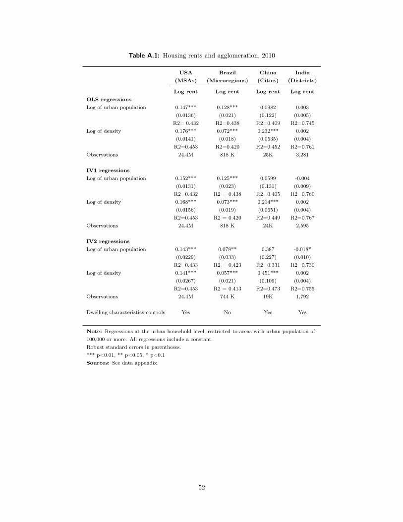
Table A.1: Housing rents and agglomeration, 2010
USA Brazil China India(MSAs) (Microregions) (Cities) (Districts)
Log rent Log rent Log rent Log rentOLS regressionsLog of urban population 0.147*** 0.128*** 0.0982 0.003
(0.0136) (0.021) (0.122) (0.005)R2= 0.432 R2=0.438 R2=0.409 R2=0.745
Log of density 0.176*** 0.072*** 0.232*** 0.002(0.0141) (0.018) (0.0535) (0.004)
R2=0.453 R2=0.420 R2=0.452 R2=0.761Observations 24.4M 818 K 25K 3,281
IV1 regressionsLog of urban population 0.152*** 0.125*** 0.0599 -0.004
(0.0131) (0.023) (0.131) (0.009)R2=0.432 R2 = 0.438 R2=0.405 R2=0.760
Log of density 0.168*** 0.073*** 0.214*** 0.002(0.0156) (0.019) (0.0651) (0.004)
R2=0.453 R2 = 0.420 R2=0.449 R2=0.767Observations 24.4M 818 K 24K 2,595
IV2 regressionsLog of urban population 0.143*** 0.078** 0.387 -0.018*
(0.0229) (0.033) (0.227) (0.010)R2=0.433 R2 = 0.423 R2=0.331 R2=0.730
Log of density 0.141*** 0.057*** 0.451*** 0.002(0.0267) (0.021) (0.109) (0.004)
R2=0.453 R2 = 0.413 R2=0.473 R2=0.755Observations 24.4M 744 K 19K 1,792
Dwelling characteristics controls Yes No Yes Yes
Note: Regressions at the urban household level, restricted to areas with urban population of100,000 or more. All regressions include a constant.Robust standard errors in parentheses.*** p<0.01, ** p<0.05, * p<0.1Sources: See data appendix.
52

B. Data Appendix
Databases Used
Acronym Database Years Source
International
WDI World Development Indicators, The World Bank 1960-2014 http://databank.worldbank.org
U.S.A.
ACS American Community Survey 5-Year sample(5-in-100 national random sample of the population)
2006-2010 https://usa.ipums.org/usa
USPC Tabulated data from the Population Census, whichmostly come from the National Historical GeographicInformation System, which in turn compiles datafrom the U.S. Census.
2010, 2000,1990, 1980
https://www.nhgis.org/
BEA Income data rural/urban from Bureau of EconomicAnalysis
2010 http://bea.gov/iTable/index_nipa.cfm
CCDB City and County Data book (amenities variables) 1990 From County and City Data book1994 (hard copy only)
BRFSS Behavioral Risk Factor Surveillance System (BRFSS)conducted by the Centers for Disease Control
From Glaeser, Gottlieb and Ziv(2014a)
Brazil
BPC Population Census micro-data sample 2010, 2000,1991, 1980
www.fflch.usp.br/centrodametropole
IPD IPEA Municipal areas and climate data 2010 www.ipeadata.gov.br
ETDB Evolution of territorial division of Brazil -municipalities microdata.
1980-2010 http://downloads.ibge.gov.br/
IPUMS Integrated Public Use Microdata series, international(IPUMS). Brazilian census
2010, 2000,1991, 1980
https://international.ipums.orgThis sample is smaller than theofficial census sample, and geographicidentifiers are less disaggregated.However, it includes homogenizedvariables that are comparable acrosstime and across countries.
China
CPSS 1% Population Sample Survey 2005
CPC China County Population Census Data with GISMaps - All China Marketing Research Co., Ltd.
2010, 2000,1990, 1982
All China Marketing Research Co.,Ltd., an agent for non-confidentialdata collected by the National Bureauof Statistics of China.
CHIPS China Household Income Project (CHIP) SurveyUrban Dataset
2007 http://www.ciidbnu.org/chip
CCSY China City Statistical Yearbook 2005, 2002
PSY Provincial Statistical Yearbook
CMA China Meteorological Administration
India
IHDS The India Human Development Survey IHDS-II 2012 www.ihds.umd.edu
IPC1 Census tables, Census of India (Office of theRegistrar General & Census Commissioner).
2011, 2001,1991
www.censusindia.gov.in
53
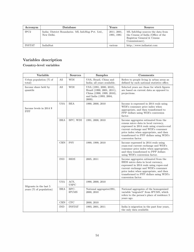
Acronym Database Years Source
IPC2 India: District Boundaries. ML InfoMap Pvt. Ltd.,New Delhi.
2011, 2001,1991, 1981
ML InfoMap sources the data fromthe Census of India (Office of theRegistrar General & CensusCommissioner).
INSTAT IndiaStat various http://www.indiastat.com
Variables descriptionCountry-level variables
Variable Sources Samples Comments
Urban population (% oftotal)
All WDI USA, Brazil, China andIndia; all years available.
Refers to people living in urban areas asdefined by each national statistics office.
Income share held byquantile
All WDI USA (1991, 2000, 2010),Brazil (1990, 2001, 2011),China (1990, 1999, 2010),and India (1993, 2004,2009).
Selected years are those for which figuresare based on current data as opposed toprojections.
Income levels in 2014 $PPP
USA BEA 1990, 2000, 2010 Income is expressed in 2014 reals usingWDI’s consumer price index whenappropriate, and then transformed toPPP dollars using WDI’s conversionfactor.
BRA BPC, WDI 1991, 2000, 2010 Income aggregates estimated from thecensus micro data in local currency,expressed in 2014 reals using cruzeiro-realcurrent exchange and WDI’s consumerprice index when appropriate, and thentransformed to PPP dollars using WDI’sconversion factor.
CHN PSY 1990, 1999, 2010 Income expressed in 2014 reals usingyuan-real current exchange and WDI’sconsumer price index when appropriate,and then transformed to PPP dollarsusing WDI’s conversion factor.
IND IHDS 2005, 2011 Income aggregates estimated from theIHDS micro data in local currency,expressed in 2014 reals using rupee-realcurrent exchange and WDI’s consumerprice index when appropriate, and thentransformed to PPP dollars using WDI’sconversion factor.
Migrants in the last 5years (% of population)
USA ACS,USPC
1990, 2000, 2010
BRA BPC-IPUMS
National aggregates1991,2000, 2010
National aggregates of the homogenizedvariable “migrate5” from IPUMS, whichrefers to the person’s place of residence 5years ago.
CHN CPC 2000, 2010
IND INSTAT 1993, 2001, 2011 India is migration in the past four years,the only data available.
54
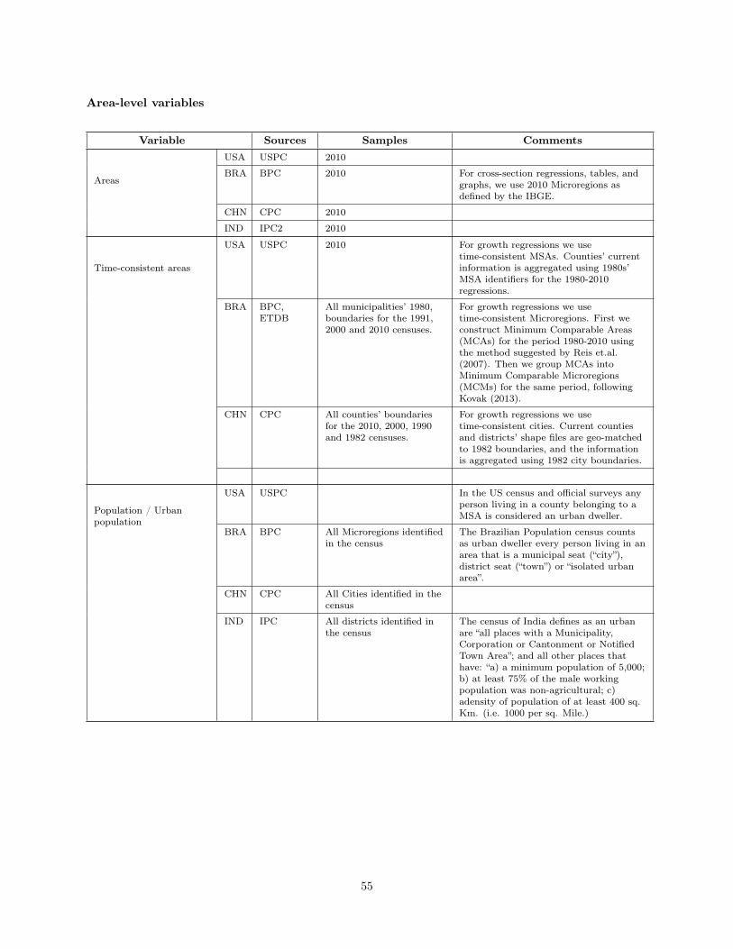
Area-level variables
Variable Sources Samples Comments
Areas
USA USPC 2010
BRA BPC 2010 For cross-section regressions, tables, andgraphs, we use 2010 Microregions asdefined by the IBGE.
CHN CPC 2010
IND IPC2 2010
Time-consistent areas
USA USPC 2010 For growth regressions we usetime-consistent MSAs. Counties’ currentinformation is aggregated using 1980s’MSA identifiers for the 1980-2010regressions.
BRA BPC,ETDB
All municipalities’ 1980,boundaries for the 1991,2000 and 2010 censuses.
For growth regressions we usetime-consistent Microregions. First weconstruct Minimum Comparable Areas(MCAs) for the period 1980-2010 usingthe method suggested by Reis et.al.(2007). Then we group MCAs intoMinimum Comparable Microregions(MCMs) for the same period, followingKovak (2013).
CHN CPC All counties’ boundariesfor the 2010, 2000, 1990and 1982 censuses.
For growth regressions we usetime-consistent cities. Current countiesand districts’ shape files are geo-matchedto 1982 boundaries, and the informationis aggregated using 1982 city boundaries.
Population / Urbanpopulation
USA USPC In the US census and official surveys anyperson living in a county belonging to aMSA is considered an urban dweller.
BRA BPC All Microregions identifiedin the census
The Brazilian Population census countsas urban dweller every person living in anarea that is a municipal seat (“city”),district seat (“town”) or “isolated urbanarea”.
CHN CPC All Cities identified in thecensus
IND IPC All districts identified inthe census
The census of India defines as an urbanare “all places with a Municipality,Corporation or Cantonment or NotifiedTown Area”; and all other places thathave: “a) a minimum population of 5,000;b) at least 75% of the male workingpopulation was non-agricultural; c)adensity of population of at least 400 sq.Km. (i.e. 1000 per sq. Mile.)
55
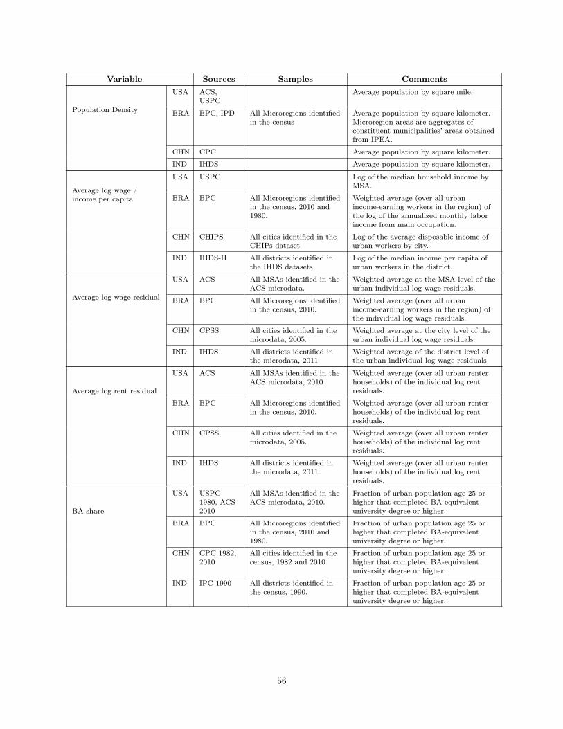
Variable Sources Samples Comments
Population Density
USA ACS,USPC
Average population by square mile.
BRA BPC, IPD All Microregions identifiedin the census
Average population by square kilometer.Microregion areas are aggregates ofconstituent municipalities’ areas obtainedfrom IPEA.
CHN CPC Average population by square kilometer.
IND IHDS Average population by square kilometer.
Average log wage /income per capita
USA USPC Log of the median household income byMSA.
BRA BPC All Microregions identifiedin the census, 2010 and1980.
Weighted average (over all urbanincome-earning workers in the region) ofthe log of the annualized monthly laborincome from main occupation.
CHN CHIPS All cities identified in theCHIPs dataset
Log of the average disposable income ofurban workers by city.
IND IHDS-II All districts identified inthe IHDS datasets
Log of the median income per capita ofurban workers in the district.
Average log wage residual
USA ACS All MSAs identified in theACS microdata.
Weighted average at the MSA level of theurban individual log wage residuals.
BRA BPC All Microregions identifiedin the census, 2010.
Weighted average (over all urbanincome-earning workers in the region) ofthe individual log wage residuals.
CHN CPSS All cities identified in themicrodata, 2005.
Weighted average at the city level of theurban individual log wage residuals.
IND IHDS All districts identified inthe microdata, 2011
Weighted average of the district level ofthe urban individual log wage residuals
Average log rent residual
USA ACS All MSAs identified in theACS microdata, 2010.
Weighted average (over all urban renterhouseholds) of the individual log rentresiduals.
BRA BPC All Microregions identifiedin the census, 2010.
Weighted average (over all urban renterhouseholds) of the individual log rentresiduals.
CHN CPSS All cities identified in themicrodata, 2005.
Weighted average (over all urban renterhouseholds) of the individual log rentresiduals.
IND IHDS All districts identified inthe microdata, 2011.
Weighted average (over all urban renterhouseholds) of the individual log rentresiduals.
BA share
USA USPC1980, ACS2010
All MSAs identified in theACS microdata, 2010.
Fraction of urban population age 25 orhigher that completed BA-equivalentuniversity degree or higher.
BRA BPC All Microregions identifiedin the census, 2010 and1980.
Fraction of urban population age 25 orhigher that completed BA-equivalentuniversity degree or higher.
CHN CPC 1982,2010
All cities identified in thecensus, 1982 and 2010.
Fraction of urban population age 25 orhigher that completed BA-equivalentuniversity degree or higher.
IND IPC 1990 All districts identified inthe census, 1990.
Fraction of urban population age 25 orhigher that completed BA-equivalentuniversity degree or higher.
56
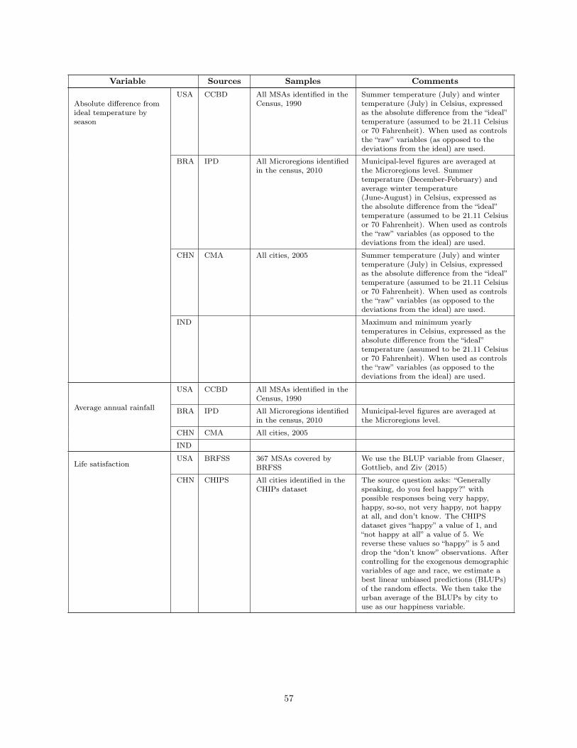
Variable Sources Samples Comments
Absolute difference fromideal temperature byseason
USA CCBD All MSAs identified in theCensus, 1990
Summer temperature (July) and wintertemperature (July) in Celsius, expressedas the absolute difference from the “ideal”temperature (assumed to be 21.11 Celsiusor 70 Fahrenheit). When used as controlsthe “raw” variables (as opposed to thedeviations from the ideal) are used.
BRA IPD All Microregions identifiedin the census, 2010
Municipal-level figures are averaged atthe Microregions level. Summertemperature (December-February) andaverage winter temperature(June-August) in Celsius, expressed asthe absolute difference from the “ideal”temperature (assumed to be 21.11 Celsiusor 70 Fahrenheit). When used as controlsthe “raw” variables (as opposed to thedeviations from the ideal) are used.
CHN CMA All cities, 2005 Summer temperature (July) and wintertemperature (July) in Celsius, expressedas the absolute difference from the “ideal”temperature (assumed to be 21.11 Celsiusor 70 Fahrenheit). When used as controlsthe “raw” variables (as opposed to thedeviations from the ideal) are used.
IND Maximum and minimum yearlytemperatures in Celsius, expressed as theabsolute difference from the “ideal”temperature (assumed to be 21.11 Celsiusor 70 Fahrenheit). When used as controlsthe “raw” variables (as opposed to thedeviations from the ideal) are used.
Average annual rainfall
USA CCBD All MSAs identified in theCensus, 1990
BRA IPD All Microregions identifiedin the census, 2010
Municipal-level figures are averaged atthe Microregions level.
CHN CMA All cities, 2005
IND
Life satisfactionUSA BRFSS 367 MSAs covered by
BRFSSWe use the BLUP variable from Glaeser,Gottlieb, and Ziv (2015)
CHN CHIPS All cities identified in theCHIPs dataset
The source question asks: “Generallyspeaking, do you feel happy?” withpossible responses being very happy,happy, so-so, not very happy, not happyat all, and don’t know. The CHIPSdataset gives “happy” a value of 1, and“not happy at all” a value of 5. Wereverse these values so “happy” is 5 anddrop the “don’t know” observations. Aftercontrolling for the exogenous demographicvariables of age and race, we estimate abest linear unbiased predictions (BLUPs)of the random effects. We then take theurban average of the BLUPs by city touse as our happiness variable.
57
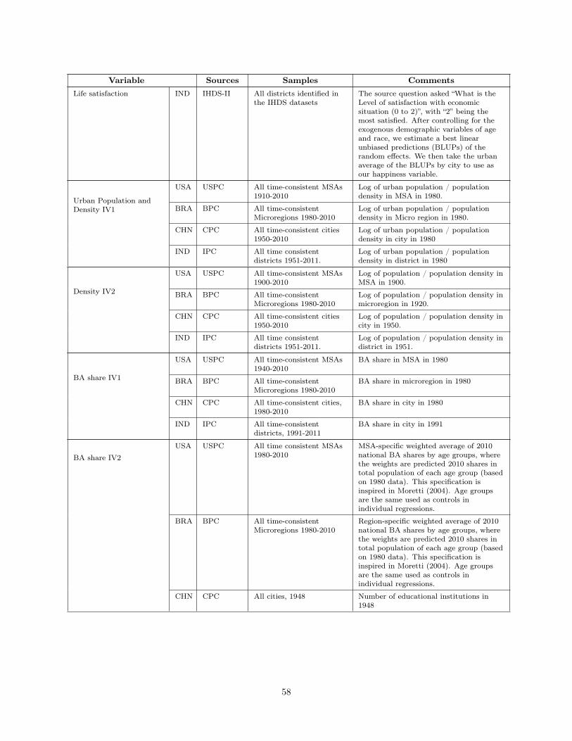
Variable Sources Samples Comments
Life satisfaction IND IHDS-II All districts identified inthe IHDS datasets
The source question asked “What is theLevel of satisfaction with economicsituation (0 to 2)”, with “2” being themost satisfied. After controlling for theexogenous demographic variables of ageand race, we estimate a best linearunbiased predictions (BLUPs) of therandom effects. We then take the urbanaverage of the BLUPs by city to use asour happiness variable.
Urban Population andDensity IV1
USA USPC All time-consistent MSAs1910-2010
Log of urban population / populationdensity in MSA in 1980.
BRA BPC All time-consistentMicroregions 1980-2010
Log of urban population / populationdensity in Micro region in 1980.
CHN CPC All time-consistent cities1950-2010
Log of urban population / populationdensity in city in 1980
IND IPC All time consistentdistricts 1951-2011.
Log of urban population / populationdensity in district in 1980
Density IV2
USA USPC All time-consistent MSAs1900-2010
Log of population / population density inMSA in 1900.
BRA BPC All time-consistentMicroregions 1980-2010
Log of population / population density inmicroregion in 1920.
CHN CPC All time-consistent cities1950-2010
Log of population / population density incity in 1950.
IND IPC All time consistentdistricts 1951-2011.
Log of population / population density indistrict in 1951.
BA share IV1
USA USPC All time-consistent MSAs1940-2010
BA share in MSA in 1980
BRA BPC All time-consistentMicroregions 1980-2010
BA share in microregion in 1980
CHN CPC All time-consistent cities,1980-2010
BA share in city in 1980
IND IPC All time-consistentdistricts, 1991-2011
BA share in city in 1991
BA share IV2USA USPC All time consistent MSAs
1980-2010MSA-specific weighted average of 2010national BA shares by age groups, wherethe weights are predicted 2010 shares intotal population of each age group (basedon 1980 data). This specification isinspired in Moretti (2004). Age groupsare the same used as controls inindividual regressions.
BRA BPC All time-consistentMicroregions 1980-2010
Region-specific weighted average of 2010national BA shares by age groups, wherethe weights are predicted 2010 shares intotal population of each age group (basedon 1980 data). This specification isinspired in Moretti (2004). Age groupsare the same used as controls inindividual regressions.
CHN CPC All cities, 1948 Number of educational institutions in1948
58
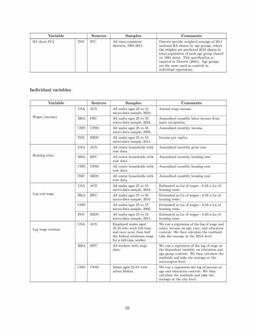
Variable Sources Samples Comments
BA share IV2 IND IPC All time-consistentdistricts, 1991-2011
District-specific weighted average of 2011national BA shares by age groups, wherethe weights are predicted 2010 shares intotal population of each age group (basedon 1991 data). This specification isinspired in Moretti (2004). Age groupsare the same used as controls inindividual regressions.
Individual variables
Variable Sources Samples Comments
Wages (income)
USA ACS All males ages 25 to 55micro-data sample, 2010.
Annual wage income.
BRA PBC All males ages 25 to 55micro-data sample, 2010.
Annualized monthly labor income frommain occupation.
CHN CPSS All males ages 25 to 55micro-data sample, 2005.
Annualized monthly income.
IND IHDS All males ages 25 to 55micro-data sample, 2011.
Income per capita.
Housing rents
USA ACS All renter households withrent data.
Annualized monthly gross rent.
BRA BPC All renter households withrent data.
Annualized monthly housing rent
CHN CPSS All renter households withrent data.
Annualized monthly housing rent
IND IHDS All renter households withrent data.
Annualized monthly housing rent
Log real wage
USA ACS All males ages 25 to 55micro-data sample, 2010.
Estimated as Ln of wages - 0.33 x Ln ofhousing rents
BRA BPC All males ages 25 to 55micro-data sample, 2010
Estimated as Ln of wages - 0.33 x Ln ofhousing rents
CHN All males ages 25 to 55micro-data sample, 2005.
Estimated as Ln of wages - 0.33 x Ln ofhousing rents
IND IHDS All males ages 25 to 55micro-data sample, 2011.
Estimated as Ln of wages - 0.33 x Ln ofhousing rents
Log wage residualUSA ACS Employed males aged
25-55 who work full-timeand earn more than halfthe federal minimum wagefor a full-time worker.
We run a regression of the log of wage andsalary income on age, race, and educationcontrols. We then calculate the residualstake the average at the MSA level.
BRA BPC All workers with wagedata.
We run a regression of the log of wage asthe dependent variable, on education andage group controls. We then calculate theresiduals and take the average at themicroregion level.
CHN CPSS Males aged 25-55 withurban Hukou.
We run a regression the log of income onage and education controls. We thencalculate the residuals and take theaverage at the city level.
59
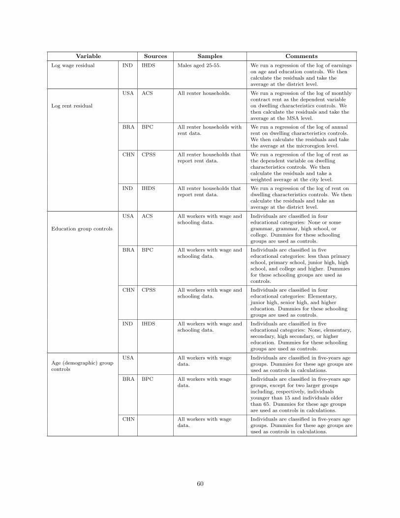
Variable Sources Samples Comments
Log wage residual IND IHDS Males aged 25-55. We run a regression of the log of earningson age and education controls. We thencalculate the residuals and take theaverage at the district level.
Log rent residual
USA ACS All renter households. We run a regression of the log of monthlycontract rent as the dependent variableon dwelling characteristics controls. Wethen calculate the residuals and take theaverage at the MSA level.
BRA BPC All renter households withrent data.
We run a regression of the log of annualrent on dwelling characteristics controls.We then calculate the residuals and takethe average at the microregion level.
CHN CPSS All renter households thatreport rent data.
We run a regression of the log of rent asthe dependent variable on dwellingcharacteristics controls. We thencalculate the residuals and take aweighted average at the city level.
IND IHDS All renter households thatreport rent data.
We run a regression of the log of rent ondwelling characteristics controls. We thencalculate the residuals and take anaverage at the district level.
Education group controls
USA ACS All workers with wage andschooling data.
Individuals are classified in foureducational categories: None or somegrammar, grammar, high school, orcollege. Dummies for these schoolinggroups are used as controls.
BRA BPC All workers with wage andschooling data.
Individuals are classified in fiveeducational categories: less than primaryschool, primary school, junior high, highschool, and college and higher. Dummiesfor these schooling groups are used ascontrols.
CHN CPSS All workers with wage andschooling data.
Individuals are classified in foureducational categories: Elementary,junior high, senior high, and highereducation. Dummies for these schoolinggroups are used as controls.
IND IHDS All workers with wage andschooling data.
Individuals are classified in fiveeducational categories: None, elementary,secondary, high secondary, or highereducation. Dummies for these schoolinggroups are used as controls.
Age (demographic) groupcontrols
USA All workers with wagedata.
Individuals are classified in five-years agegroups. Dummies for these age groups areused as controls in calculations.
BRA BPC All workers with wagedata.
Individuals are classified in five-years agegroups, except for two larger groupsincluding, respectively, individualsyounger than 15 and individuals olderthan 65. Dummies for these age groupsare used as controls in calculations.
CHN All workers with wagedata.
Individuals are classified in five-years agegroups. Dummies for these age groups areused as controls in calculations.
60
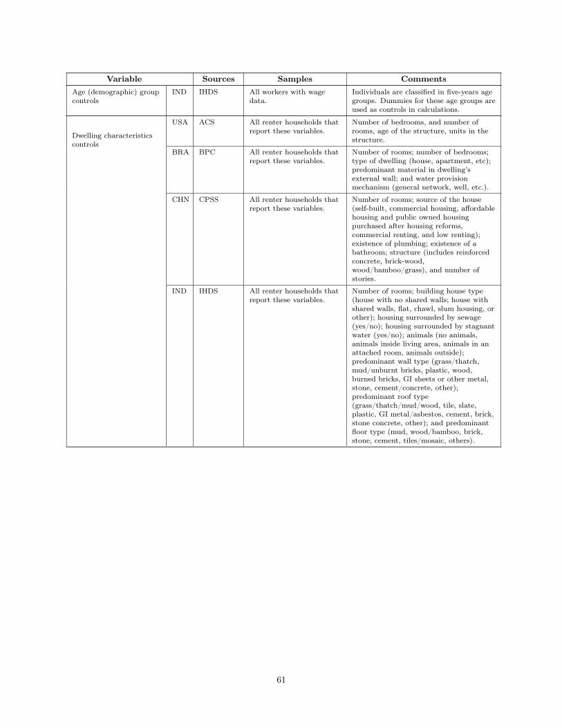
Variable Sources Samples Comments
Age (demographic) groupcontrols
IND IHDS All workers with wagedata.
Individuals are classified in five-years agegroups. Dummies for these age groups areused as controls in calculations.
Dwelling characteristicscontrols
USA ACS All renter households thatreport these variables.
Number of bedrooms, and number ofrooms, age of the structure, units in thestructure.
BRA BPC All renter households thatreport these variables.
Number of rooms; number of bedrooms;type of dwelling (house, apartment, etc);predominant material in dwelling’sexternal wall; and water provisionmechanism (general network, well, etc.).
CHN CPSS All renter households thatreport these variables.
Number of rooms; source of the house(self-built, commercial housing, affordablehousing and public owned housingpurchased after housing reforms,commercial renting, and low renting);existence of plumbing; existence of abathroom; structure (includes reinforcedconcrete, brick-wood,wood/bamboo/grass), and number ofstories.
IND IHDS All renter households thatreport these variables.
Number of rooms; building house type(house with no shared walls; house withshared walls, flat, chawl, slum housing, orother); housing surrounded by sewage(yes/no); housing surrounded by stagnantwater (yes/no); animals (no animals,animals inside living area, animals in anattached room, animals outside);predominant wall type (grass/thatch,mud/unburnt bricks, plastic, wood,burned bricks, GI sheets or other metal,stone, cement/concrete, other);predominant roof type(grass/thatch/mud/wood, tile, slate,plastic, GI metal/asbestos, cement, brick,stone concrete, other); and predominantfloor type (mud, wood/bamboo, brick,stone, cement, tiles/mosaic, others).
61