What is Classification? Classification = Learning a Modelzaiane/courses/cau/slides/cau... ·...

33459-01: Principles of Knowledge Discovery in Data – March-June, 2006 (Dr. O. Zaiane) 1

Clustering Analysis: Agglomerative, Hierarchical, Density-based and

other approaches

Lecture 6 Week 10 (May 12) and Week 11 (May 19)

33459-01 Principles of Knowledge Discovery in Data

Lecture by: Dr. Osmar R. Zaïane


• Introduction to Data Mining• Association analysis• Sequential Pattern Analysis• Classification and prediction • Contrast Sets• Data Clustering• Outlier Detection• Web Mining

Course Content


What is Classification?

1 2 3 4 n…

The goal of data classification is to organize and categorize data in distinct classes.

A model is first created based on the data distribution.The model is then used to classify new data.Given the model, a class can be predicted for new data.

?

With classification, I can predict in which bucket to put the ball, but I can’t predict the weight of the ball.


Classification = Learning a ModelTraining Set (labeled)

ClassificationModel

New unlabeled data Labeling=Classification


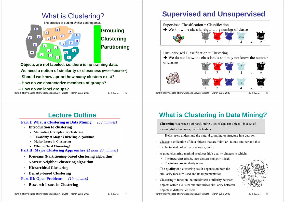
What is Clustering?

GroupingClusteringPartitioning

–Objects are not labeled, i.e. there is no training data. –We need a notion of similarity or closeness (what features?)

– Should we know apriori how many clusters exist?– How do we characterize members of groups?– How do we label groups?

a

aaa

aab

bbb

cc

c

dd

dd

d

d

e

e

e

e

e

The process of putting similar data together.


Supervised and Unsupervised

1 2 3 4 n…

Supervised Classification = ClassificationWe know the class labels and the number of classes

Unsupervised Classification = ClusteringWe do not know the class labels and may not know the number

of classes

1 2 3 4 n…???? ?

1 2 3 4 ?…???? ?

blackgreenblueredgray


Lecture Outline• Introduction to clustering

• Motivating Examples for clustering• Taxonomy of Major Clustering Algorithms• Major Issues in Clustering• What is Good Clustering?

• K-means (Partitioning-based clustering algorithm)• Nearest Neighbor clustering algorithm• Hierarchical Clustering• Density-based Clustering

• Research Issues in Clustering

Part I: What is Clustering in Data Mining (30 minutes)

Part II: Major Clustering Approaches (1 hour 20 minutes)

Part III: Open Problems (10 minutes)


What is Clustering in Data Mining?Clustering is a process of partitioning a set of data (or objects) in a set of

meaningful sub-classes, called clusters.

– Helps users understand the natural grouping or structure in a data set.

• Cluster: a collection of data objects that are “similar” to one another and thus

can be treated collectively as one group.

• A good clustering method produces high quality clusters in which:• The intra-class (that is, intraintra-cluster) similarity is high.• The inter-class similarity is low.

• The quality of a clustering result depends on both the similarity measure used and its implementation.

• Clustering = function that maximizes similarity between objects within a cluster and minimizes similarity between objects in different clusters.


Typical Clustering Applications

• As a stand-alone tool to – get insight into data distribution – find the characteristics of each cluster – assign the cluster of a new example

• As a preprocessing step for other algorithms– e.g. numerosity reduction – using cluster centers to

represent data in clusters• It is a building block for many data mining

solutions– e.g. Recommender systems – group users with similar

behaviour or preferences to improve recommendation.


Clustering Example – Fitting Troops• Fitting the troops – re-design of uniforms for female

soldiers in US army– Goal: reduce the number of uniform sizes to be kept in

inventory while still providing good fit

• Researchers from Cornell University used clustering and designed a new set of sizes – Traditional clothing size system: ordered set of graduated sizes

where all dimensions increase together– The new system: sizes that fit body types

• E.g. one size for short-legged, small waisted, women with wide and long torsos, average arms, broad shoulders, and skinny necks


Other Examples of Clustering Applications• Marketing

– help discover distinct groups of customers, and then use this knowledge to develop targeted marketing programs

• Biology – derive plant and animal taxonomies– find genes with similar function

• Land use– identify areas of similar land use in an earth observation database

• Insurance– identify groups of motor insurance policy holders with a high average

claim cost• City-planning

– identify groups of houses according to their house type, value, and geographical location


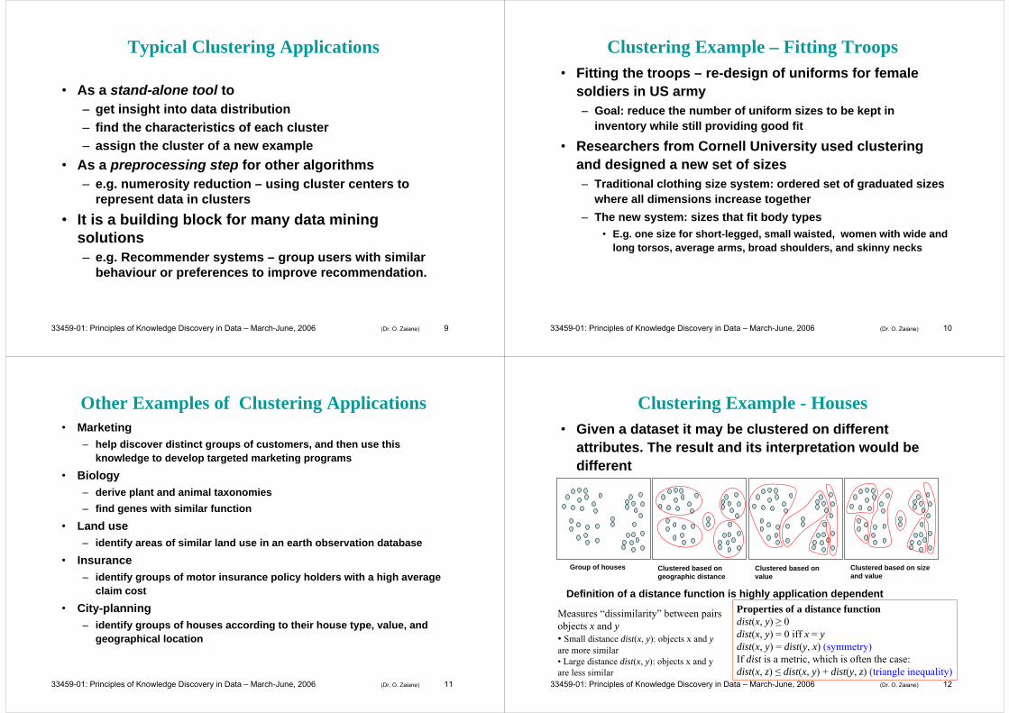
Clustering Example - Houses• Given a dataset it may be clustered on different

attributes. The result and its interpretation would be different

Group of houses Clustered based on geographic distance

Clustered based on value

Clustered based on size and value

Definition of a distance function is highly application dependent Properties of a distance functiondist(x, y) ≥ 0dist(x, y) = 0 iff x = ydist(x, y) = dist(y, x) (symmetry)If dist is a metric, which is often the case:dist(x, z) ≤ dist(x, y) + dist(y, z) (triangle inequality)

Measures “dissimilarity” between pairs objects x and y• Small distance dist(x, y): objects x and y are more similar• Large distance dist(x, y): objects x and y are less similar


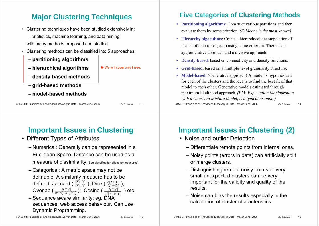
Major Clustering Techniques• Clustering techniques have been studied extensively in:

– Statistics, machine learning, and data mining

with many methods proposed and studied.

• Clustering methods can be classified into 5 approaches:

– partitioning algorithms– hierarchical algorithms– density-based methods– grid-based methods– model-based methods

We will cover only these.


Five Categories of Clustering Methods• Partitioning algorithms: Construct various partitions and then

evaluate them by some criterion. (K-Means is the most known)

• Hierarchy algorithms: Create a hierarchical decomposition of the set of data (or objects) using some criterion. There is an agglomerative approach and a divisive approach.

• Density-based: based on connectivity and density functions.

• Grid-based: based on a multiple-level granularity structure.• Model-based: (Generative approach) A model is hypothesized

for each of the clusters and the idea is to find the best fit of that model to each other. Generative models estimated through maximum likelihood approach. (EM: Expectation Maximization with a Gaussian Mixture Model, is a typical example)


Important Issues in Clustering• Different Types of Attributes

– Numerical: Generally can be represented in a Euclidean Space. Distance can be used as a measure of dissimilarity.(See classification slides for measures)

– Categorical: A metric space may not be definable. A similarity measure has to be defined. Jaccard ( ); Dice ( ); Overlap ( ); Cosine ( ) etc.

– Sequence aware similarity: eg. DNA sequences, web access behaviour. Can use Dynamic Programming.


Important Issues in Clustering (2)• Noise and outlier Detection

– Differentiate remote points from internal ones.– Noisy points (errors in data) can artificially split

or merge clusters.– Distinguishing remote noisy points or very

small unexpected clusters can be very important for the validity and quality of the results.

– Noise can bias the results especially in the calculation of cluster characteristics.


Important Issues in Clustering (3)• High dimensional spaces

– The more dimensions describe the data the sparser the space is. The sparser the space the smaller the likelihood to discover significant clusters.

– Large number of dimensions makes it hard to process.

– What is the meaning of distance or similarity in a high dimensional space?

– Indexes are not efficient– The curse of dimensionality


Important Issues in Clustering (4)• Parameters

– Clustering algorithms are typically VERY sensitive to parameters. A small delta makes a huge difference in the final results.

– Tuning is very difficult.– Parameters are not necessarily related to the

application domain– E.g. The best number of clusters to discover (k) is not known

• There is no one correct answer to a clustering problem• domain expertise is required


Requirements of Clustering inData Mining

• Scalability (very large number of objects to cluster)

• Dealing with different types of attributes (Numeric & categorical)

• Discovery of clusters with arbitrary shape

• Minimal requirements for domain knowledge to determine input parameters (minimize parameters)

• Able to deal with noise and outliers

• Insensitive to order of input records

• Handles high dimensionality

• Can be incremental for dynamic change

Not all Clustering Algorithms can deal with all these requirements. They target some of them and ignore the others by making assumptions and imposing approximations.










Partitioning Algorithms: Basic Concept

• Partitioning method: Construct a partition of a database Dof N objects into a set of k clusters.

• Given a k, find a partition of k clusters that optimizes the chosen partitioning criterion. – Global optimal: exhaustively enumerate all partitions.

– Heuristic methods: k-means and k-medoids algorithms.

– k-means (MacQueen’67): Each cluster is represented by the center of the cluster.

– k-medoids or PAM (Partition around medoids) (Kaufman & Rousseeuw ’87): Each cluster is represented by one of the objects in the cluster.

Partitioning

K-nn

Hierarchical

Density-based

Requires the number of clusters k to be pre-specified


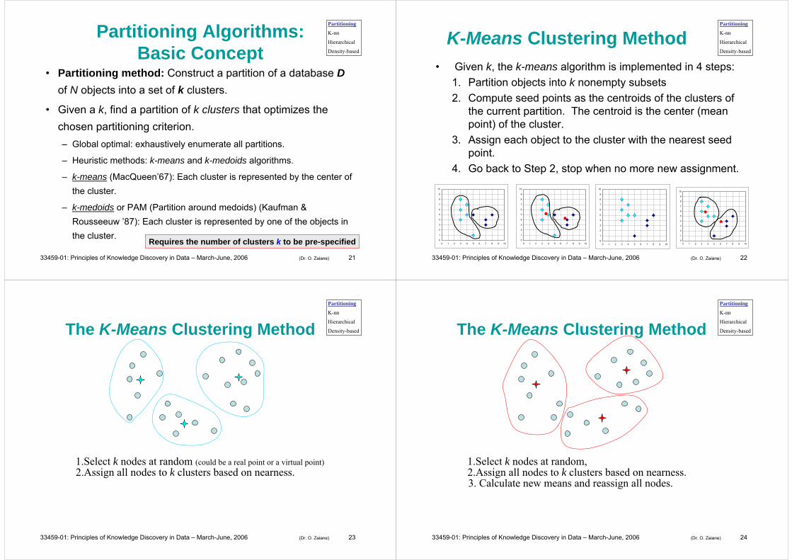
K-Means Clustering Method• Given k, the k-means algorithm is implemented in 4 steps:

1. Partition objects into k nonempty subsets2. Compute seed points as the centroids of the clusters of

the current partition. The centroid is the center (mean point) of the cluster.

3. Assign each object to the cluster with the nearest seed point.

4. Go back to Step 2, stop when no more new assignment.

0

1

2

3

4

5

6

7

8

9

10

0 1 2 3 4 5 6 7 8 9 100

1

2

3

4

5

6

7

8

9

10

0 1 2 3 4 5 6 7 8 9 100

1

2

3

4

5

6

7

8

9

10

0 1 2 3 4 5 6 7 8 9 100

1

2

3

4

5

6

7

8

9

10

0 1 2 3 4 5 6 7 8 9 10

Partitioning

K-nn

Hierarchical

Density-based


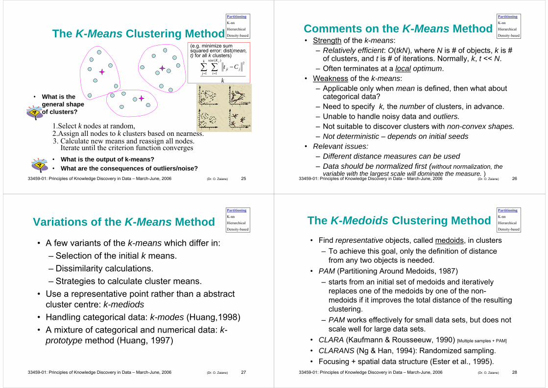
The K-Means Clustering Method

1.Select k nodes at random (could be a real point or a virtual point)2.Assign all nodes to k clusters based on nearness.

Partitioning

K-nn

Hierarchical

Density-based



1.Select k nodes at random,

3. Calculate new means and reassign all nodes.

Partitioning

K-nn

Hierarchical

Density-based

2.Assign all nodes to k clusters based on nearness.



Iterate until the criterion function converges

Partitioning

K-nn

Hierarchical

Density-based

1.Select k nodes at random,

3. Calculate new means and reassign all nodes.2.Assign all nodes to k clusters based on nearness.

• What is the output of k-means?• What are the consequences of outliers/noise?

(e.g. minimize sum squared error: dist(mean, t) for all k clusters)

• What is the general shape of clusters?

k

Ctk

j

Ksize

ijji

j

∑ ∑= =

−1

)(

1

2


Comments on the K-Means Method• Strength of the k-means:

– Relatively efficient: O(tkN), where N is # of objects, k is # of clusters, and t is # of iterations. Normally, k, t << N.

– Often terminates at a local optimum. • Weakness of the k-means:

– Applicable only when mean is defined, then what about categorical data?

– Need to specify k, the number of clusters, in advance.– Unable to handle noisy data and outliers.– Not suitable to discover clusters with non-convex shapes.– Not deterministic – depends on initial seeds

• Relevant issues:– Different distance measures can be used– Data should be normalized first (without normalization, the

variable with the largest scale will dominate the measure. )

Partitioning

K-nn

Hierarchical

Density-based


Variations of the K-Means Method

• A few variants of the k-means which differ in:– Selection of the initial k means.– Dissimilarity calculations.– Strategies to calculate cluster means.

• Use a representative point rather than a abstract cluster centre: k-mediods

• Handling categorical data: k-modes (Huang,1998)• A mixture of categorical and numerical data: k-

prototype method (Huang, 1997)

Partitioning

K-nn

Hierarchical

Density-based


The K-Medoids Clustering Method• Find representative objects, called medoids, in clusters

– To achieve this goal, only the definition of distance from any two objects is needed.

• PAM (Partitioning Around Medoids, 1987)– starts from an initial set of medoids and iteratively

replaces one of the medoids by one of the non-medoids if it improves the total distance of the resulting clustering.

– PAM works effectively for small data sets, but does not scale well for large data sets.

• CLARA (Kaufmann & Rousseeuw, 1990) [Multiple samples + PAM]

• CLARANS (Ng & Han, 1994): Randomized sampling.• Focusing + spatial data structure (Ester et al., 1995).

Partitioning

K-nn

Hierarchical

Density-based


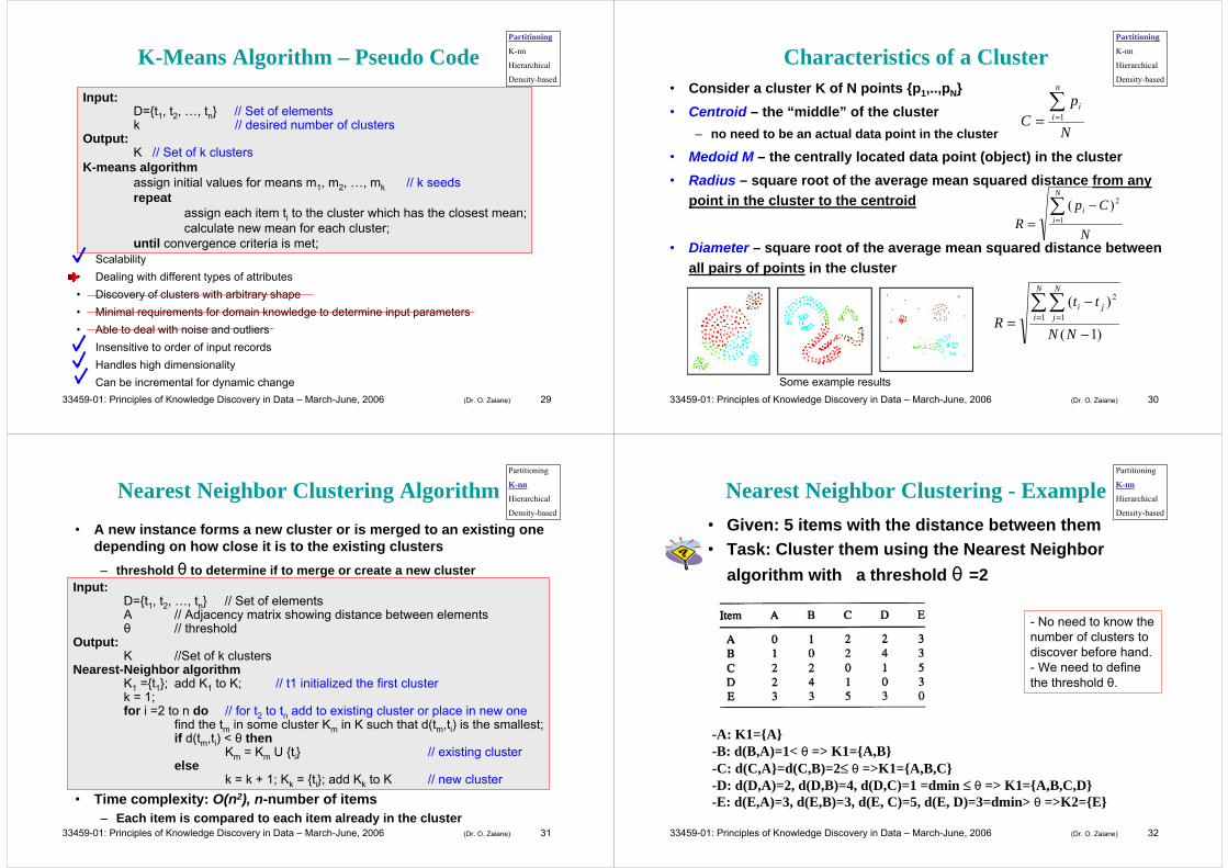
K-Means Algorithm – Pseudo CodeInput:

D={t1, t2, …, tn} // Set of elementsk // desired number of clusters

Output:K // Set of k clusters

K-means algorithmassign initial values for means m1, m2, …, mk // k seedsrepeat

assign each item ti to the cluster which has the closest mean;calculate new mean for each cluster;

until convergence criteria is met;• Scalability • Dealing with different types of attributes • Discovery of clusters with arbitrary shape• Minimal requirements for domain knowledge to determine input parameters • Able to deal with noise and outliers• Insensitive to order of input records• Handles high dimensionality• Can be incremental for dynamic change

Partitioning

K-nn

Hierarchical

Density-based


Characteristics of a Cluster• Consider a cluster K of N points {p1,..,pN}• Centroid – the “middle” of the cluster

– no need to be an actual data point in the cluster

• Medoid M – the centrally located data point (object) in the cluster • Radius – square root of the average mean squared distance from any

point in the cluster to the centroid

• Diameter – square root of the average mean squared distance between all pairs of points in the cluster

N

pC

n

ii∑

== 1

N

CpR

N

ii∑

=

−= 1

2)(

)1(

)(1 1

2

−

−=∑∑

= =

NN

ttR

N

i

N

jji

Some example results

Partitioning

K-nn

Hierarchical

Density-based


Nearest Neighbor Clustering Algorithm• A new instance forms a new cluster or is merged to an existing one

depending on how close it is to the existing clusters– threshold θ to determine if to merge or create a new cluster

• Time complexity: O(n2), n-number of items– Each item is compared to each item already in the cluster

Partitioning

K-nn

Hierarchical

Density-based

Input:D={t1, t2, …, tn} // Set of elementsA // Adjacency matrix showing distance between elementsθ // threshold

Output:K //Set of k clusters

Nearest-Neighbor algorithmK1 ={t1}; add K1 to K; // t1 initialized the first clusterk = 1;for i =2 to n do // for t2 to tn add to existing cluster or place in new one

find the tm in some cluster Km in K such that d(tm,ti) is the smallest;if d(tm,ti) < θ then

Km = Km U {ti} // existing clusterelse

k = k + 1; Kk = {ti}; add Kk to K // new cluster


Nearest Neighbor Clustering - Example• Given: 5 items with the distance between them• Task: Cluster them using the Nearest Neighbor

algorithm with a threshold θ =2

-A: K1={A}-B: d(B,A)=1< θ => K1={A,B}-C: d(C,A}=d(C,B)=2≤ θ =>K1={A,B,C}-D: d(D,A)=2, d(D,B)=4, d(D,C)=1 =dmin ≤ θ => K1={A,B,C,D}-E: d(E,A)=3, d(E,B)=3, d(E, C)=5, d(E, D)=3=dmin> θ =>K2={E}

Partitioning

K-nn

Hierarchical

Density-based

- No need to know the number of clusters to discover before hand. - We need to define the threshold θ.


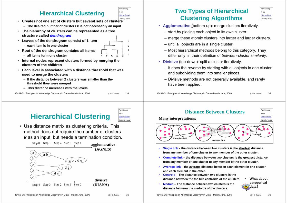
Hierarchical Clustering• Creates not one set of clusters but several sets of clusters

– The desired number of clusters k is not necessarily an input• The hierarchy of clusters can be represented as a tree

structure called dendrogram• Leaves of the dendrogram consist of 1 item

– each item is in one cluster• Root of the dendrogram contains all items

– all items form one cluster• Internal nodes represent clusters formed by merging the

clusters of the children• Each level is associated with a distance threshold that was

used to merge the clusters – If the distance between 2 clusters was smaller than the

threshold they were merged– This distance increases with the levels.

Partitioning

K-nn

Hierarchical

Density-based


Two Types of Hierarchical Clustering Algorithms

• Agglomerative (bottom-up): merge clusters iteratively.– start by placing each object in its own cluster. – merge these atomic clusters into larger and larger clusters. – until all objects are in a single cluster. – Most hierarchical methods belong to this category. They

differ only in their definition of between-cluster similarity.• Divisive (top-down): split a cluster iteratively.

– It does the reverse by starting with all objects in one cluster and subdividing them into smaller pieces.

– Divisive methods are not generally available, and rarely have been applied.

Partitioning

K-nn

Hierarchical

Density-based


Hierarchical Clustering• Use distance matrix as clustering criteria. This

method does not require the number of clusters k as an input, but needs a termination condition.

Step 0 Step 1 Step 2 Step 3 Step 4

b

dc

e

a a b

d ec d e

a b c d e

Step 4 Step 3 Step 2 Step 1 Step 0

agglomerative(AGNES)

divisive(DIANA)

Partitioning

K-nn

Hierarchical

Density-based


Distance Between Clusters

Single link

Complete link

• Single link – the distance between two clusters is the shortest distance from any member of one cluster to any member of the other cluster.

• Complete link – the distance between two clusters is the greatest distance from any member of one cluster to any member of the other cluster.

• Average link – the average distance between each element in one cluster and each element in the other.

Many interpretations:

Average link

Medoid

Centroidx

x

Partitioning

K-nn

Hierarchical

Density-based

• What about categorical data?

• Centroid – The distance between two clusters is the distance between the the two centroids of the clusters

• Medoid – The distance between two clusters is the distance between the medoids of the clusters.


AGNES (Agglomerative Nesting)• Introduced in Kaufmann and Rousseeuw (1990)• Implemented in statistical analysis packages, such

as S+.• Use the Single-Link method and the dissimilarity

matrix. • Merge nodes that have the least dissimilarity• Go on in a non-descending fashion• Eventually all nodes belong to the same cluster

0

1

2

3

4

5

6

7

8

9

10

0 1 2 3 4 5 6 7 8 9 10

0

1

2

3

4

5

6

7

8

9

10

0 1 2 3 4 5 6 7 8 9 10

0

1

2

3

4

5

6

7

8

9

10

0 1 2 3 4 5 6 7 8 9 10

Partitioning

K-nn

Hierarchical

Density-based


DIANA (Divisive Analysis)

• Introduced in Kaufmann and Rousseeuw (1990)

• Implemented in statistical analysis packages, such as S+.

• Inverse order of AGNES.

• Eventually each node forms a cluster on its own.

0

1

2

3

4

5

6

7

8

9

10

0 1 2 3 4 5 6 7 8 9 100

1

2

3

4

5

6

7

8

9

10

0 1 2 3 4 5 6 7 8 9 10

0

1

2

3

4

5

6

7

8

9

10

0 1 2 3 4 5 6 7 8 9 10

Partitioning

K-nn

Hierarchical

Density-based


Dendrogram Representation• A set of ordered triples (d,k,K)

– d is the distance threshold value– k is the number of clusters– K is the set of clusters

• Example{ ( 0, 5, {{A},{B},{C}, {D}, {E}} ),

(1, 3, {{A,B}, {C,D}, {E}} ),(2, 2, {{A,B,C,D}, {E}} ),(3, 1, {A,B,C,D,E}} ) }

• Thus, the output is not one set of clusters but several. One can determine which of the sets to use.

A B C D E 0123

Partitioning

K-nn

Hierarchical

Density-based


Agglomerative Algorithms – Pseudo Code• Different algorithms merge clusters at each level differently

(procedure NewClusters)• Merge only 2 or

more clusters?• If there are several

clusters with identical distances, which ones to merge?

• How to determine the distance between clusters? – single link– complete link– average link

Threshold distanceNum. of clustersSet of clusters

A[i,j]=distance(ti,tj)

May be different than 1

Partitioning

K-nn

Hierarchical

Density-based


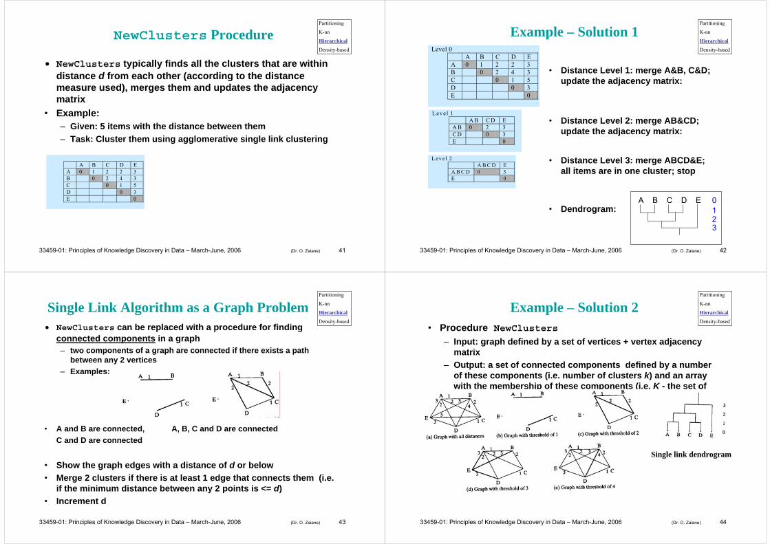
NewClusters Procedure

• NewClusters typically finds all the clusters that are within distance d from each other (according to the distance measure used), merges them and updates the adjacency matrix

• Example: – Given: 5 items with the distance between them– Task: Cluster them using agglomerative single link clustering

A B C D E A 0 1 2 2 3 B 0 2 4 3 C 0 1 5 D 0 3 E 0

Partitioning

K-nn

Hierarchical

Density-based


Example – Solution 1Level 0

A B C D E A 0 1 2 2 3 B 0 2 4 3 C 0 1 5 D 0 3 E 0

Level 1

A B C D E A B 0 2 3 C D 0 3 E 0

L ev e l 2 A B C D E A B C D 0 3 E 0

• Distance Level 1: merge A&B, C&D; update the adjacency matrix:

• Distance Level 2: merge AB&CD; update the adjacency matrix:

• Distance Level 3: merge ABCD&E; all items are in one cluster; stop

• Dendrogram:

Partitioning

K-nn

Hierarchical

Density-based

A B C D E 0123


Single Link Algorithm as a Graph Problem• NewClusters can be replaced with a procedure for finding

connected components in a graph– two components of a graph are connected if there exists a path

between any 2 vertices– Examples:

• A and B are connected, A, B, C and D are connectedC and D are connected

• Show the graph edges with a distance of d or below• Merge 2 clusters if there is at least 1 edge that connects them (i.e.

if the minimum distance between any 2 points is <= d)• Increment d

Partitioning

K-nn

Hierarchical

Density-based


Example – Solution 2• Procedure NewClusters

– Input: graph defined by a set of vertices + vertex adjacency matrix

– Output: a set of connected components defined by a number of these components (i.e. number of clusters k) and an array with the membership of these components (i.e. K - the set of clusters)

Single link dendrogram

Partitioning

K-nn

Hierarchical

Density-based


Single Link vs. Complete Link Algorithm• Single link suffers from the so called chain effect

– 2 clusters are merged if only 2 of their points are close to each other– there may be points in the 2 clusters that are far from each other but this

has no effect on the algorithm – Thus the clusters may contain points that are not related to each other

but simply happen to be near points that are close to each other

• Complete link – the distance between 2 clusters is the largestdistance between an element in one cluster and an element in another– Generates more compact clusters– Dendrogram for the example

Partitioning

K-nn

Hierarchical

Density-based


Average Link• Average link - the distance between 2 clusters is the

average distance between an element in one cluster and an element in another

arbitrary set; can be 1

For our example

Partitioning

K-nn

Hierarchical

Density-based


Applicability and Complexity

• Hierarchical clustering algorithms are suitable for domains with natural nesting relationships between clusters– Biology- plant and animal taxonomies can be viewed as a

hierarchy of clusters• Space complexity of the algorithm: O(n2), n - number of

items– The space required to store the adjacency distance matrix

• Space complexity of the dendrogram: O(kn), k-number of levels

• Time complexity of the algorithm: O(kn2) – 1 iteration for each level of the dendrogram

• Not incremental – assume all data is present

Partitioning

K-nn

Hierarchical

Density-based


Density-Based Clustering Methods

• Clustering based on density (local cluster criterion), such as density-connected points.

• Major features:– Discover clusters of arbitrary shape– Handle noise– One scan– Need density parameters as termination condition

• Several interesting studies:– DBSCAN: Ester, et al. (KDD ’96)– DENCLUE: Hinneburg & D. Keim (KDD ’98)– CLIQUE: Agrawal, et al. (SIGMOD ’98)– OPTICS: Ankerst, et al (SIGMOD ’99).– TURN*: Foss and Zaïane (ICDM ’02)

Partitioning

K-nn

Hierarchical

Density-based


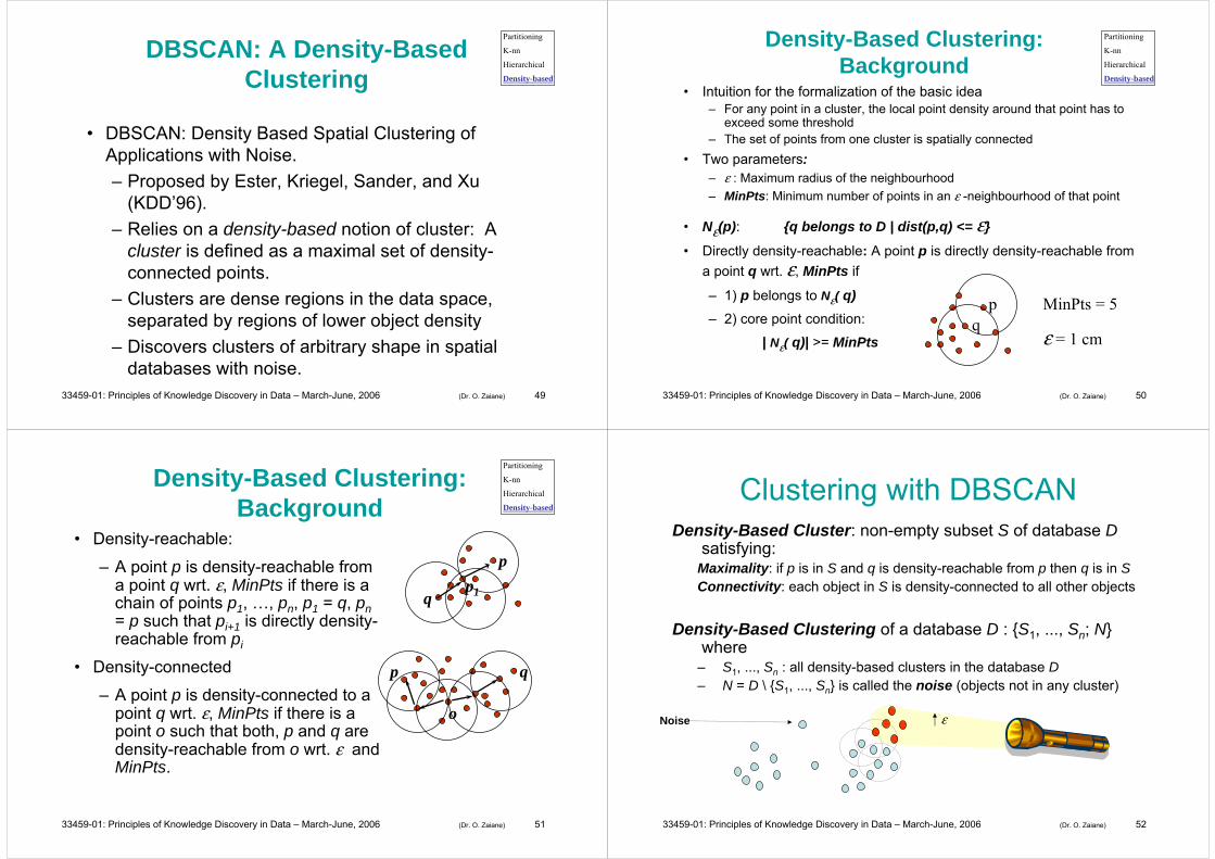
DBSCAN: A Density-Based Clustering

• DBSCAN: Density Based Spatial Clustering of Applications with Noise.– Proposed by Ester, Kriegel, Sander, and Xu

(KDD’96). – Relies on a density-based notion of cluster: A

cluster is defined as a maximal set of density-connected points.

– Clusters are dense regions in the data space, separated by regions of lower object density

– Discovers clusters of arbitrary shape in spatial databases with noise.

Partitioning

K-nn

Hierarchical

Density-based


Density-Based Clustering: Background

• Intuition for the formalization of the basic idea– For any point in a cluster, the local point density around that point has to

exceed some threshold– The set of points from one cluster is spatially connected

• Two parameters:– ε : Maximum radius of the neighbourhood– MinPts: Minimum number of points in an ε -neighbourhood of that point

• Nε(p): {q belongs to D | dist(p,q) <= ε}

• Directly density-reachable: A point p is directly density-reachable from a point q wrt. ε, MinPts if

– 1) p belongs to Nε( q)– 2) core point condition:

| Nε( q)| >= MinPts

pq

MinPts = 5

ε = 1 cm

Partitioning

K-nn

Hierarchical

Density-based


Density-Based Clustering: Background

• Density-reachable:

– A point p is density-reachable from a point q wrt. ε, MinPts if there is a chain of points p1, …, pn, p1 = q, pn= p such that pi+1 is directly density-reachable from pi

• Density-connected

– A point p is density-connected to a point q wrt. ε, MinPts if there is a point o such that both, p and q are density-reachable from o wrt. ε and MinPts.

p q

o

p

qp1

Partitioning

K-nn

Hierarchical

Density-based


Clustering with DBSCANDensity-Based Cluster: non-empty subset S of database D

satisfying:Maximality: if p is in S and q is density-reachable from p then q is in SConnectivity: each object in S is density-connected to all other objects

Density-Based Clustering of a database D : {S1, ..., Sn; N} where

– S1, ..., Sn : all density-based clusters in the database D– N = D \ {S1, ..., Sn} is called the noise (objects not in any cluster)

εNoise


DBSCAN General Algorithmfor each o ∈ D do

if o is not yet labeled thenif o is a core-object then

collect all objects density-reachable from oand assign them to a new cluster.

elseassign o to NOISE

density-reachable objects are collected by performing successive ε-neighborhood queries.


DBSCAN Advantages and Disadvantages

Advantages• Clusters can have arbitrary shape and size• Number of clusters is determined automatically• Can separate clusters from surrounding noise• Can be supported by spatial index structuresDisadvantages• Input parameters may be difficult to determine• Very sensitive to input parameter setting

Runtime complexitiesNε-query DBSCAN

without support (worst case): O(n) O(n2 )tree-based support (e.g. R*-tree) : O(log(n)) O(n ∗ log(n) )direct access to the neighborhood: O(1) O(n)

Partitioning

K-nn

Hierarchical

Density-based


Wish list (DBScan)

• Scalability • Dealing with different types of attributes • Discovery of clusters with arbitrary shape• Minimal requirements for domain knowledge to determine input parameters • Able to deal with noise and outliers• Insensitive to order of input records• Handles high dimensionality• Can be incremental for dynamic change

Partitioning

K-nn

Hierarchical

Density-based


TURN* (Foss and Zaiane, 2002)

• TURN* contains several sub-algorithms.• TURN-RES computes a clustering of spatial data at a given resolution based on a definition of ‘close’ neighbours: di – dj <= 1.0 for two points i, j and a local density ti based on a point’s distances to its nearest axial neighbours: ti = Σd=0

D f(dd) for dimensions D.• This density based approach is fast, identifies clusters of arbitrary shape and isolates noise.

Partitioning

K-nn

Hierarchical

Density-based


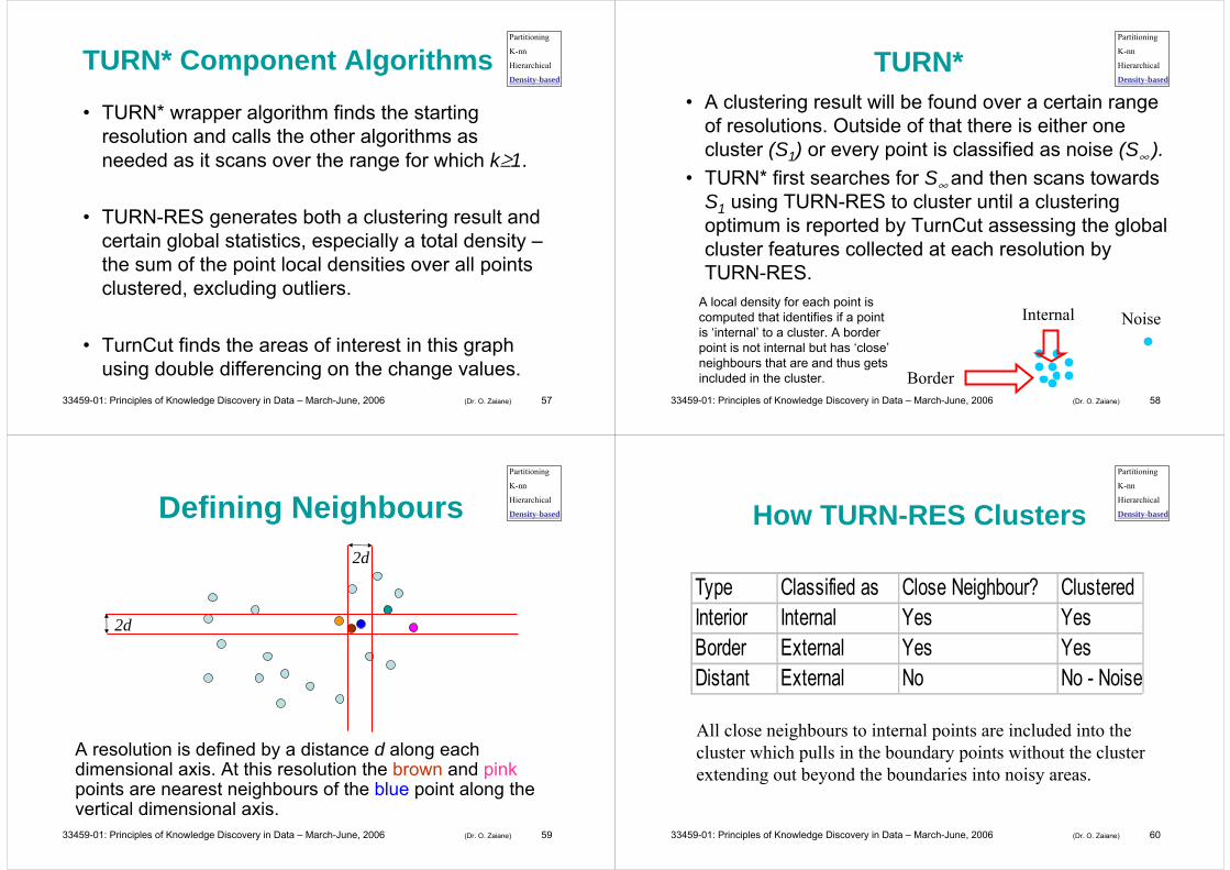
TURN* Component Algorithms

• TURN* wrapper algorithm finds the starting resolution and calls the other algorithms as needed as it scans over the range for which k≥1.

• TURN-RES generates both a clustering result and certain global statistics, especially a total density –the sum of the point local densities over all points clustered, excluding outliers.

• TurnCut finds the areas of interest in this graph using double differencing on the change values.

Partitioning

K-nn

Hierarchical

Density-based


TURN*• A clustering result will be found over a certain range

of resolutions. Outside of that there is either one cluster (S1) or every point is classified as noise (S∞ ).

• TURN* first searches for S∞ and then scans towards S1 using TURN-RES to cluster until a clustering optimum is reported by TurnCut assessing the global cluster features collected at each resolution by TURN-RES.

Partitioning

K-nn

Hierarchical

Density-based

Noise

Border

InternalA local density for each point is computed that identifies if a point is ‘internal’ to a cluster. A border point is not internal but has ‘close’neighbours that are and thus gets included in the cluster.


Defining Neighbours

A resolution is defined by a distance d along each dimensional axis. At this resolution the brown and pinkpoints are nearest neighbours of the blue point along the vertical dimensional axis.

2d

2d

Partitioning

K-nn

Hierarchical

Density-based


How TURN-RES Clusters

Type Classified as Close Neighbour? ClusteredInterior Internal Yes YesBorder External Yes YesDistant External No No - Noise

All close neighbours to internal points are included into the cluster which pulls in the boundary points without the cluster extending out beyond the boundaries into noisy areas.

Partitioning

K-nn

Hierarchical

Density-based


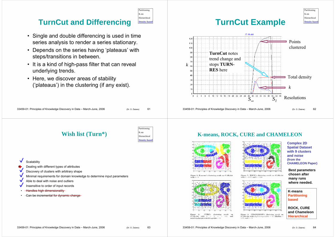
TurnCut and Differencing• Single and double differencing is used in time

series analysis to render a series stationary.• Depends on the series having ‘plateaus’ with

steps/transitions in between.• It is a kind of high-pass filter that can reveal

underlying trends.• Here, we discover areas of stability

(‘plateaus’) in the clustering (if any exist).

Partitioning

K-nn

Hierarchical

Density-based


TurnCut Example

Resolutions

Points clustered

Total density

k

TurnCut notes trend change and stops TURN-RES here

k

S1S∞

Partitioning

K-nn

Hierarchical

Density-based


Wish list (Turn*)

• Scalability • Dealing with different types of attributes • Discovery of clusters with arbitrary shape• Minimal requirements for domain knowledge to determine input parameters • Able to deal with noise and outliers• Insensitive to order of input records• Handles high dimensionality• Can be incremental for dynamic change

Partitioning

K-nn

Hierarchical

Density-based


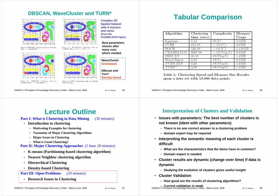
K-means, ROCK, CURE and CHAMELEON

Best parameters chosen after many runs where needed.

Complex 2D Spatial Dataset with 9 clusters and noise(from the CHAMELEON Paper)

K-meansPartitioning based

ROCK, CURE and Chameleon Hierarchical


DBSCAN, WaveCluster and TURN*

12

Best parameters chosen after many runs where needed.

Complex 2D Spatial Dataset with 9 clusters and noise(from the CHAMELEON Paper)

WaveClusterGrid-based

DBscan and Turn* Density-based


Tabular Comparison










Interpretation of Clusters and Validation• Issues with parameters: The best number of clusters is

not known (idem with other parameters)– There is no one correct answer to a clustering problem– domain expert may be required

• Interpreting the semantic meaning of each cluster is difficult– What are the characteristics that the items have in common?– Domain expert is needed

• Cluster results are dynamic (change over time) if data is dynamic – Studying the evolution of clusters gives useful insight

• Cluster Validation– How good are the results of clustering algorithms?– Current validation is weak


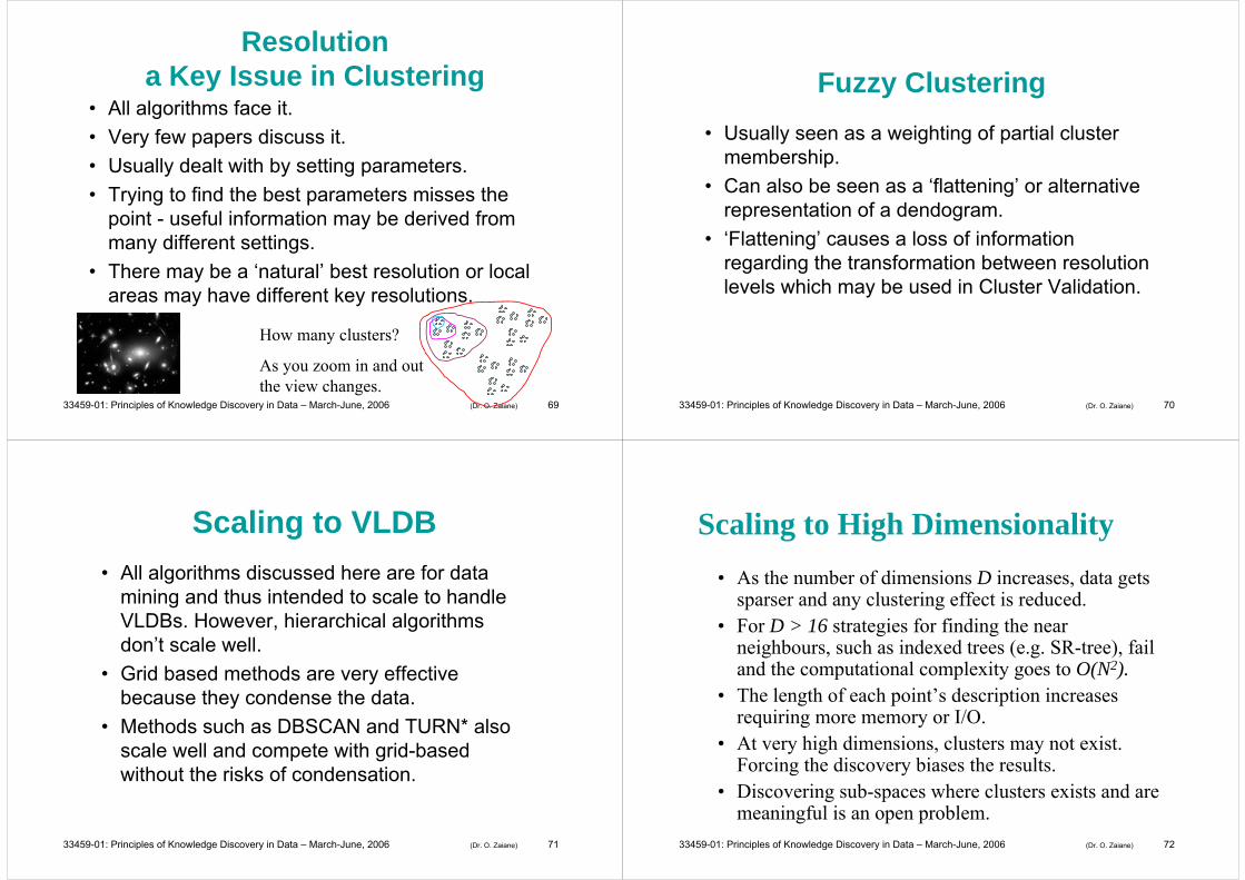
Resolutiona Key Issue in Clustering

• All algorithms face it.• Very few papers discuss it.• Usually dealt with by setting parameters.• Trying to find the best parameters misses the

point - useful information may be derived from many different settings.

• There may be a ‘natural’ best resolution or local areas may have different key resolutions.

How many clusters?

As you zoom in and out the view changes.


Fuzzy Clustering• Usually seen as a weighting of partial cluster

membership.• Can also be seen as a ‘flattening’ or alternative

representation of a dendogram.• ‘Flattening’ causes a loss of information

regarding the transformation between resolution levels which may be used in Cluster Validation.


Scaling to VLDB• All algorithms discussed here are for data

mining and thus intended to scale to handle VLDBs. However, hierarchical algorithms don’t scale well.

• Grid based methods are very effective because they condense the data.

• Methods such as DBSCAN and TURN* also scale well and compete with grid-based without the risks of condensation.


Scaling to High Dimensionality• As the number of dimensions D increases, data gets

sparser and any clustering effect is reduced.• For D > 16 strategies for finding the near

neighbours, such as indexed trees (e.g. SR-tree), fail and the computational complexity goes to O(N2).

• The length of each point’s description increases requiring more memory or I/O.

• At very high dimensions, clusters may not exist. Forcing the discovery biases the results.

• Discovering sub-spaces where clusters exists and are meaningful is an open problem.


Constraint Based Clustering• Constraints may dictate the clustering in a real

application. The algorithm should consider them (constraints on the cluster or the members in a cluster)

• In spatial data: Bridges (connecting points) or obstacles (such as rivers and highways)

• Adding features to the constraints (bridge length, wall size, etc.).

• Some solutions exist:AUTOCLUST+ (Estivill-Castro and Lee, 2000)

Based on graph partitioning

COD-CLARANS (Tung, Hou, and Han, 2001)Based on CLARANS – partitioning

DBCluC (Zaïane and Lee, 2002)Based on DBSCAN – density based


Motivating Concepts - Obstacles

• Physical Constraints (Obstacle and Crossing)

– An Obstacle -Disconnectivity functionality• A polygon denoted by P (V, E) where V is a set of points

from an obstacle and E is a set of line segments • Types: Convex and Concave.• Visibility

– Relation between two data points, if the line segment drawn from one point to the other is not intersected with a polygon P (V, E) representing a given obstacle.


Motivating Concepts - Crossings

• Crossing – Connectivity functionality– Entry point

• a point p on the perimeter of the polygon crossing, from which when a given point r is density-reachable wrt. Eps, r becomes reachable by any other point q density-reachable from any other entry point of the same crossing wrt. Eps

– Entry edge• an edge of a crossing polygon with a set of entry points starting

from one endpoint of the edge to the other separated by an interval value ie where ie ≤ Eps

• A Crossing is a set B of m entry points B={b1, b2, b3, …, bm}generated from all entry edges


Motivating Concepts - Cluster

• Cluster

– A set C of points C={ c1, c2, c3, …, cc}, satisfying the followings, where ci, cj ∈ C, C⊆D, i≠j, and 1≤i, j ≤ n

• Maximality: ∀ di, dj, if di ∈ C and dj is density-reachable from di with respect to Eps and MinPts, then dj ∈ C.

• Connectivity: ∀ ci, cj ∈ C, ci is density-connected to cj with respect to Eps and MinPts.

• ∀ ci, cj ∈ C, ci and cj are visible to each other • Crossing connectivity: If Cm and Ck are connected by a bridge

B, then a cluster Cl the union of Cm and Ck is created. Cl = Cm∪ Ck, where Cm and Ck are a set of data points. l ≠ m ≠ k


Modeling Constraints – Obstacles• Obstacle Modeling

– Objectives• Disconnectivity Functionality.• Enhance performance of processing obstacles.

– Polygon Reduction Algorithm • Represents an obstacle as a set of Obstruction Lines.• Two steps – Convex Point Test and Convex Test• Inspiration

– Maintain a set of visible spaces* created by an obstacle.


Modeling ConstraintsPolygon Reduction Algorithm

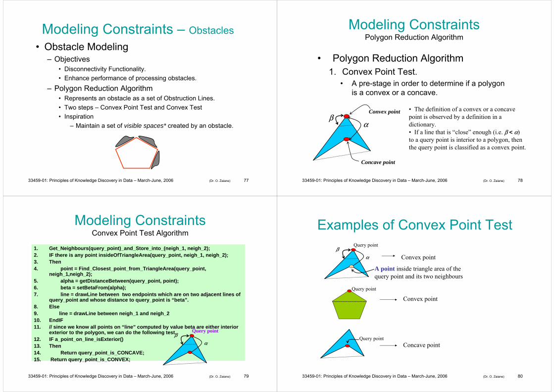
• Polygon Reduction Algorithm1. Convex Point Test.

• A pre-stage in order to determine if a polygon is a convex or a concave.

Convex point

Concave point

α

• The definition of a convex or a concave point is observed by a definition in a dictionary.• If a line that is “close” enough (i.e. β < α) to a query point is interior to a polygon, then the query point is classified as a convex point.

β


Modeling ConstraintsConvex Point Test Algorithm

1. Get_Neighbours(query_point)_and_Store_into_(neigh_1, neigh_2);2. IF there is any point insideOfTriangleArea(query_point, neigh_1, neigh_2);3. Then 4. point = Find_Closest_point_from_TriangleArea(query_point,

neigh_1,neigh_2);5. alpha = getDistanceBetween(query_point, point);6. beta = setBetaFrom(alpha);7. line = drawLine between two endpoints which are on two adjacent lines of

query_point and whose distance to query_point is “beta”.8. Else9. line = drawLine between neigh_1 and neigh_210. EndIF11. // since we know all points on “line” computed by value beta are either interior

exterior to the polygon, we can do the following test.12. IF a_point_on_line_isExterior()13. Then 14. Return query_point_is_CONCAVE;15. Return query_point_is_CONVEX;

αβ

Query point


Examples of Convex Point TestQuery point

Query point

Convex point

Concave pointQuery point

αβ

Convex point

A point inside triangle area of the query point and its two neighbours


Modeling Constraints– Polygon Reduction Algorithm

1. Convex Test - Determine if a polygon is a convex or a concave.

– A polygon is Concave if ∃ a concave point in the polygon.

– A polygon is Convex if ∀ points are convex points.

• Convex - ⎡n/2⎤ obstruction lines*.

• Concave – The number of obstruction lines depends on a shape of a given polygon.

5 3 10 3


Modeling Constraints – Crossings

• Crossing Modeling– Objective

• Connectivity functionality.• Control Flow of data.

– A polygon with Entry Points and Entry Edge.

– Defined by users or applications Eps

Entry Points


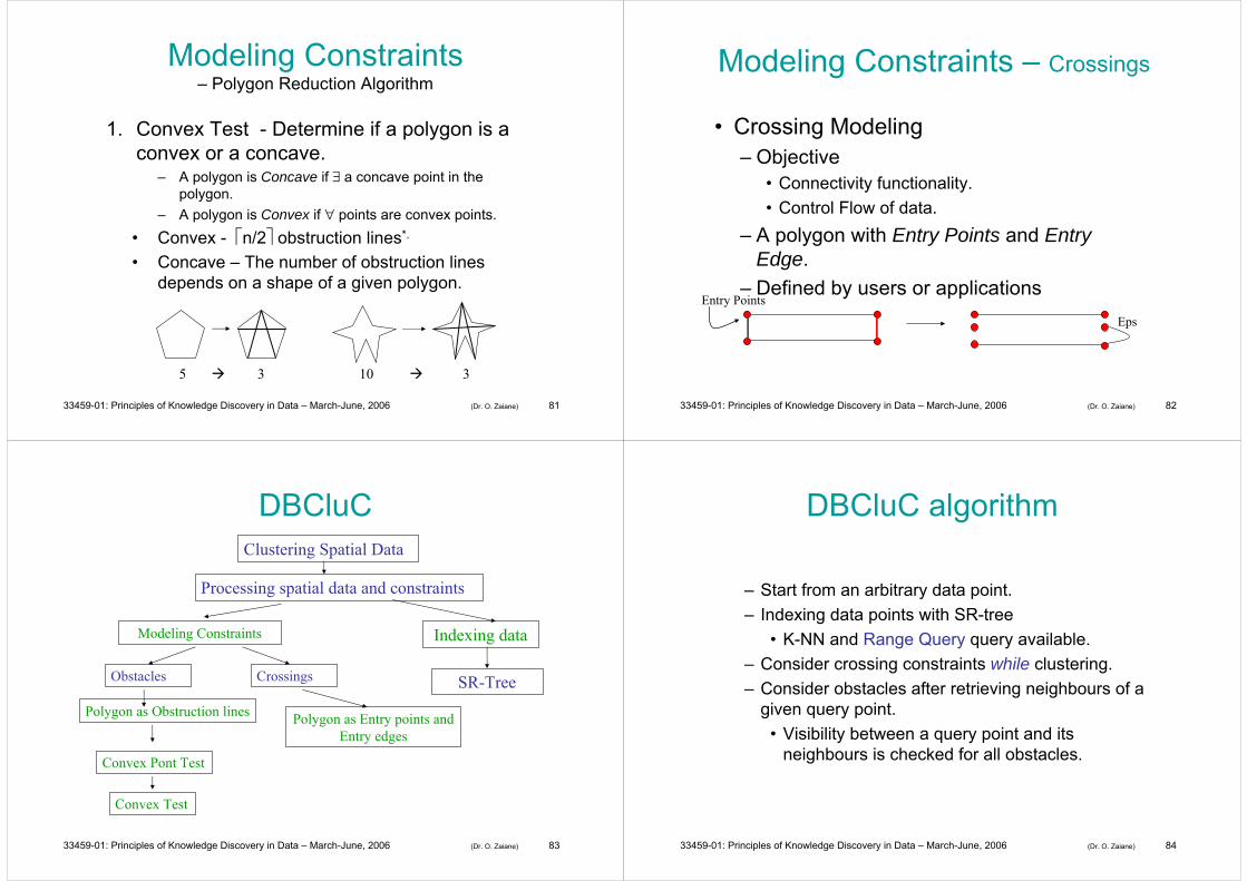
DBCluCClustering Spatial Data

Processing spatial data and constraints

Modeling Constraints Indexing data

Obstacles

Polygon as Obstruction lines

Convex Pont Test

Convex Test

SR-TreeCrossings

Polygon as Entry points and Entry edges


DBCluC algorithm

– Start from an arbitrary data point.– Indexing data points with SR-tree

• K-NN and Range Query query available.– Consider crossing constraints while clustering.– Consider obstacles after retrieving neighbours of a

given query point.• Visibility between a query point and its

neighbours is checked for all obstacles.


DBCluC - algorithmDBCluC {

// While clustering, bridges are taken into account1. START CLUSTERING FROM BRIDGE ENTRY POINTS2. FOR REMAINING DATA POINTS Point FROM A Database3. IF ExpandCluster (Database,Point, ClusterId, Eps, MinPts, Obstacles)

THEN4. ClusterId = nextId(ClusterId)5. END IF6. END FOR}

• Complexity - Polygon Reduction Algorithm O(n2), where n is the number of points of the

largest polygon in terms of edges.

- DBCluC – O(N*logN*L), where N is the number of data points and L is the number of obstruction lines.


Some Illustrative Results

(a) Before clustering (b) Clustering ignoring constraints (a) Clustering with bridges

(a) Clustering with obstacles (a) Clustering with obstacles and bridges

What is Classification? Classification = Learning a Modelzaiane/courses/cau/slides/cau... ·...

Documents

Transcript of What is Classification? Classification = Learning a Modelzaiane/courses/cau/slides/cau... ·...