Evaluating NPV Estimates I: The Basic Problem

The basic problem: How reliable is our NPV estimate?Projected vs. Actual cash flowsEstimated cash flows are based on a distribution of possible outcomes each periodForecasting riskThe possibility of a bad decision due to errors in cash flow projections

Sources of valueWhat conditions must exist to create the estimated NPV?

“What If” analysisA. Scenario analysisB. Sensitivity analysis

Evaluating NPV Estimates II: Scenario and Other “What-If” Analyses

Scenario and Other “What-If” Analyses“Base case” estimationEstimated NPV based on initial cash flow projectionsScenario analysisBase, best, and worst-case scenarios and calculate NPVsChange var. values (sale, Var.cost, Fixed cost…etc)

Sensitivity analysisHow does the estimated NPV change when one of the input variables changes? Freeze all other var.

Simulation analysisVary several input variables simultaneously, then construct a distribution of possible NPV estimates

Example:

Fairways Driving Range expects rentals to be 20,000 buckets at $3 per bucket. Equipment costs $20,000 and will be depreciated using SL over 5 years and have a $0 salvage value. Variable costs are 10% of rentals and fixed costs are $40,000 per year. Assume no increase in working capital nor any additional capital outlays. The required return is 15% and the tax rate is 15%.

Revenues $60,000 (3x20,000)

Variable costs 6,000 (10% rev)

Fixed costs 40,000

Depreciation 4,000 (20,000/5)

EBIT $10,000

Taxes (@15%) 1500

Net income $ 8,500

Example (concluded)

Estimated annual cash inflows:

$10,000 + 4,000 - 1,500 = $12,500

EBIT Dep. Tax

At 15%, the 5-year annuity factor is 3.352. Thus, the base-case NPV is:

NPV = $-20,000 + ($12,500 × 3.352) = $21,900.

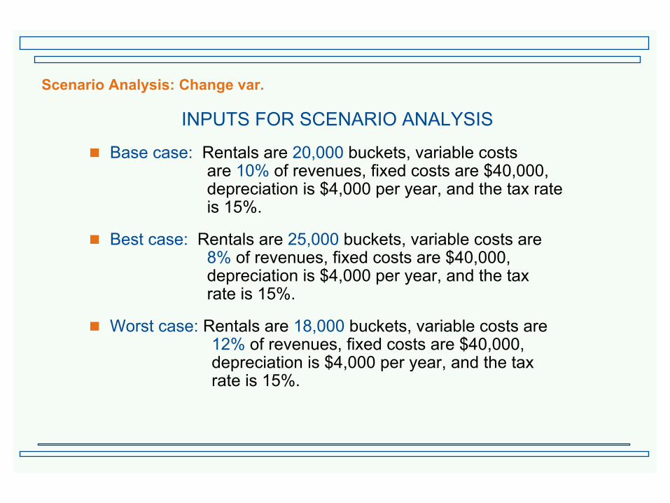
Scenario Analysis: Change var.

INPUTS FOR SCENARIO ANALYSIS

Base case: Rentals are 20,000 buckets, variable costs are 10% of revenues, fixed costs are $40,000, depreciation is $4,000 per year, and the tax rate is 15%.

Best case: Rentals are 25,000 buckets, variable costs are 8% of revenues, fixed costs are $40,000, depreciation is $4,000 per year, and the tax rate is 15%.

Worst case: Rentals are 18,000 buckets, variable costs are 12% of revenues, fixed costs are $40,000, depreciation is $4,000 per year, and the tax rate is 15%.

Scenario Analysis (concluded)

Net ProjectScenario Rentals Revenues Income Cash Flow NPV

Best Case 25,000 $75,000 $21,250 $25,250 $64,635

Base Case 20,000 60,000 8,500 12,500 21,900

Worst Case 18,000 54,000 2,992 6,992 3,437

Sensitivity Analysis: Freeze var. except for one

INPUTS FOR SENSITIVITY ANALYSIS

Base case: Rentals are 20,000 buckets, variable costs are 10% of revenues, fixed costs are $40,000, depreciation is $4,000 per year, and the tax rate is 15%.

Best case: Rentals are 25,000 buckets and revenues are $75,000. All other variables are unchanged.

Worst case: Rentals are 18,000 buckets and revenues are $54,000. All other variables are unchanged.

Sensitivity Analysis (concluded)

Net ProjectScenario Rentals Revenues income cash flow NPV

Best case 25,000 $75,000 $19,975 $23,975 $60,364

Base case 20,000 60,000 8,500 12,500 21,900

Worst case 18,000 54,000 3,910 7,910 6,514

Rentals vs. NPVSensitivity Analysis - Rentals vs. NPV

Base case

NPV = $21,900

NPV

Worst case

NPV = $6,514

Rentals per Year

Best case

NPV = $60,035

0

-$60,00015,000 25,00020,000

$60,000

x

x

x

Total Cost = Variable cost + Fixed cost

Variable Fixed Total TotalRentals Revenue cost cost cost Depr. acct. cost

0 $0 $0 $40,000 $40,000 $4,000 $44,000

15,000 45,000 4,500 40,000 44,500 4,000 48,500

20,000 60,000 6,000 40,000 46,000 4,000 50,000

25,000 75,000 7,500 40,000 47,500 4,000 51,500

Total Cost Calculations

Break-Even AnalysisFairways Break-Even Analysis - Sales vs. Costs and Rentals

Accountingbreak-even point16,296 Buckets

Rentals per Year

$50,000

$20,00015,000 25,000

$80,000

Total revenues

Fixed costs + Dep

$44,000

NetIncome < 0

NetIncome > 0

20,000

Accounting Break-Even Quantity

Accounting Break-Even Quantity (Q)

Q = (Fixed costs + Depreciation)/(Price per unit - Variable cost per unit)

= (FC + D)/(P - V)

= ($40,000 + 4,000)/($3.00 - .30)

= 16,296 buckets

If sales do not reach 16,296 buckets, the firm will incur losses in both the accounting sense and the financial sense .

Quick Quiz -- Part 1 of 2

Assume you have the following information about RJInc:

Price = $5 per unit; variable costs = $3 per unit

Fixed operating costs = $10,000

Initial cost is $20,000

5 year life; straight-line depreciation to 0, no salvage value

Assume no taxes

Required return = 20%

Part 1 of 2 (concluded)

Break-Even Computations

A. Accounting Break-Even

Q = (FC + D)/(P - V) = ($_____ + $4,000)/($5 - 3) = ______ units

IRR = ______ ; NPV ______ ( = -$______ )

B. Cash Break-Even

Q = FC/(P - V) = $10,000/($5 - 3) = ______ units

IRR = ______ ; NPV = ______

B. Financial Break-Even

Q = (FC + $6,688)/(P - V)

= ($10,000 + 6,688)/($5 - 3) = 8,344 units

IRR = ______ ; NPV = ______

Quick Quiz -- Part 1 of 2 (concluded)

Break-Even Computations

A. Accounting Break-Even (non-cash –Dep)

Q = (FC + D)/(P - V) = ($10,000 + $4,000)/($5 - 3) = 7,000 units

IRR = 0 ; NPV = -$8,038

B. Cash Break-Even

Q = FC/(P - V) = $10,000/($5 - 3) = 5,000 units

IRR = -100% ; NPV = -$20,000

B. Financial Break-Even

Q = (FC + $6,688)/(P - V)

= ($10,000 + 6,688)/($5 - 3) = 8,344 units

IRR = 20% ; NPV = 0

Summary of Break-Even Measures

I. The General Expression

Q = (FC + OCF)/(P - V)where: FC = total fixed costs

P = Price per unitv = variable cost per unit

II. The Accounting Break-Even Point

Q = (FC + D)/(P - V)

At the Accounting BEP, net income = 0, NPV is negative, and IRR of 0.

III. The Cash Break-Even Point

Q = FC/(P - V)

At the Cash BEP, operating cash flow = 0, NPV is negative, and IRR = -100%.

IV. The Financial Break-Even Point

Q = (FC + OCF*)/(P - V)

At the Financial BEP, NPV = 0 and IRR = required return.

DOL (Degree of operating leverage):

Since %∆ in OCF = DOL × % ∆ in Q, DOL is a “multiplier” which measures the effect of a change in quantity sold on OCF.

For Fairways, let Q = 20,000 buckets. Ignoring taxes,

OCF = $14,000 and fixed costs = $40,000, and

Fairway’s DOL = 1 + FC/OCF = 1 + $40,000/$14,000 = 3.857.

In other words, a 10% increase (decrease) in quantity sold will result in a 38.57% increase (decrease) in OCF.

Two points should be kept in mind:

Higher DOL suggests greater volatility (i.e., risk) in OCF;

Leverage is a two-edged sword - sales decreases will be magnified as much as increases.

Quick Quiz -- Part 2 of 2

1. What is forecasting risk?

It is the possibility that errors in projected cash flows will lead to incorrect decisions.

2. What is scenario analysis? Why might this exercise be useful fordecision-makers to perform, even if their estimates ultimately turn out to be incorrect?

It uses estimates of “Best- and Worst-case” outcomes to see what happens to NPV estimates if things turn out differently than expected. It forces decision-makers to think about the possibility of alternative outcomes.

Problem 1

BetaBlockers, Inc. (BBI) manufactures biotech sunglasses. The variable materials cost is $0.68 per unit and the variable laborcost is $2.08 per unit.

What is the variable cost per unit?

VC = variable material cost + variable labor cost

= $0.68 + $2.08 = $2.76

Suppose BBI incurs fixed costs of $520,000 during a year when production is 250,000 units. What are total costs for the year?

TC = total variable costs + fixed costs

= ($2.76)( ______ ) + $ ______ = $ ______

Solution to Problem 1

BetaBlockers, Inc. (BBI) manufactures biotech sunglasses. The variable materials cost is $0.68 per unit and the variable laborcost is $2.08 per unit.

What is the variable cost per unit?

VC = variable material cost + variable labor cost

= $0.68 + $2.08 = $2.76

Suppose BBI incurs fixed costs of $520,000 during a year when production is 250,000 units. What are total costs for the year?

TC = total variable costs + fixed costs

= ($2.76)(250,000) + $520,000 = $1,210,000

Solution to Problem 1 (concluded)

If the selling price is $6.00 per unit, does BBI break even on acash basis? If depreciation is $150,000 per year, what is the accounting break-even point?

Qcash = $520,000/($ ______ – $ ______ )

= ______ units

Qacct = ($ ______ + $ ______)/($6.00 – $2.76)

= ______ units

Solution to Problem 1 (concluded)

If the selling price is $6.00 per unit, what is the BBI break even on a cash basis? If depreciation is $150,000 per year, what is the accounting break-even point?

Qcash = $520,000/($ 6.00 – $ 2.76 )

= 160,494 units

Qacct = ($520,000 + $150,000)/($6.00 - $2.76)

= 206,790 units

Problem 2

In each of the following cases, calculate the accounting break-even and the cash break-even points. Ignore any tax effects in calculating the cash break-even.

Unit price Unit VC Fixed costs Depreciation

$1,900 $1,750 $16 million $7 million

30 26 60,000 150,000

7 2 300 365

Solution to Problem 2 (concluded)

Solutions

(1) Qacct = ($16M + $___ )/($1,900 - $1,750) = ______ units

Qcash = $16M/($_____ - $ _____ ) = 106,667 units

(2) Qacct = ($60K + $150K)/($__ - $26) = 52,500 units

Qcash = $______ /($30 - $26) = ______ units

(3) Qacct = ($300 + $365)/($7 - $2) = ___ units

Qcash = $300/($7 - $2) = 60 units

Solution to Problem 2 (concluded)

Solutions

(1) Qacct = ($16M + $ 7m )/($1,900 - $1,750) = 153,334 units

Qcash = $16M/($1,900 - $ 1,750) = 106,667 units

(2) Qacct = ($60K + $150K)/($30 - $26) = 52,500 units

Qcash = $60,000/($30 - $26) = 15,000 units

(3) Qacct = ($300 + $365)/($7 - $2) = 133 units

Qcash = $300/($7 - $2) = 60 units

Problem 3

A proposed project has fixed costs of $20,000 per year. OCF at 7,000 units is $55,000. Ignoring taxes, what is the degree of operating leverage (DOL)?

If units sold rises from 7,000 to 7,300, what will be the increase in OCF? What is the new DOL?

DOL = 1 + ($20,000/$55,000) = 1.3637

% ∆ Q = (7,300 - 7,000)/7,000 = 4.29%

and

% ∆ OCF = DOL(% ∆ Q) = ______ (4.29) = ____ %

New OCF = ($55,000)(_______ ) = $_______

DOL at 7,300 units = 1 + ($20,000/$ _______ ) = _______

Solution to Problem 3

A proposed project has fixed costs of $20,000 per year. OCF at 7,000 units is $55,000. Ignoring taxes, what is the degree of operating leverage (DOL)?

If units sold rises from 7,000 to 7,300, what will be the increase in OCF? What is the new DOL?

DOL = 1 + ($20,000/$55,000) = 1.3637

% ∆ Q = (7,300 - 7,000)/7,000 = 4.29%

and

% ∆ OCF = DOL(% ∆ Q) = 1.3637 (4.29) = 5.85%

New OCF = ($55,000)(1.0585) = $58,218

DOL at 7,300 units = 1 + ($20,000/$58,218) = 1.3435