What Happened Next? Using Deep Learning to Value DefensiveActions in Football Event-Data

Charbel MerhejUniversity of Southampton

Southampton, United Kingdomcm2u19@soton.ac.uk

Ryan J BealUniversity of Southampton

Southampton, United Kingdomryan.beal@soton.ac.uk

Tim MatthewsSentient Sports

Southampton, United Kingdomtim.matthews@sentientsports.com

Sarvapali RamchurnUniversity of Southampton

Southampton, United Kingdomsdr1@soton.ac.uk

ABSTRACTObjectively quantifying the value of player actions in football (soc-cer) is a challenging problem. To date, studies in football analyticshave mainly focused on the attacking side of the game, while therehas been less work on event-driven metrics for valuing defensiveactions (e.g., tackles and interceptions). Therefore in this paper,we use deep learning techniques to define a novel metric that val-ues such defensive actions by studying the threat of passages ofplay that preceded them. By doing so, we are able to value defen-sive actions based on what they prevented from happening in thegame. Our Defensive Action Expected Threat (DAxT) model hasbeen validated using real-world event-data from the 2017/2018 and2018/2019 English Premier League seasons, and we combine ourmodel outputs with additional features to derive an overall ratingof defensive ability for players. Overall, we find that our model isable to predict the impact of defensive actions allowing us to bettervalue defenders using event-data.

CCS CONCEPTS• Applied computing; • Computing methodologies→Modeldevelopment and analysis; Neural networks;

KEYWORDSSports Analytics; Football; Deep Learning; Neural Networks; Ap-plied Machine Learning; Defensive Actions

ACM Reference Format:Charbel Merhej, Ryan J Beal, Tim Matthews, and Sarvapali Ramchurn. 2021.What Happened Next? Using Deep Learning to Value Defensive Actionsin Football Event-Data. In Proceedings of the 27th ACM SIGKDD Conferenceon Knowledge Discovery and Data Mining (KDD ’21), August 14–18, 2021,Virtual Event, Singapore. ACM, New York, NY, USA, 10 pages. https://doi.org/10.1145/3447548.3467090

Permission to make digital or hard copies of all or part of this work for personal orclassroom use is granted without fee provided that copies are not made or distributedfor profit or commercial advantage and that copies bear this notice and the full citationon the first page. Copyrights for components of this work owned by others than ACMmust be honored. Abstracting with credit is permitted. To copy otherwise, or republish,to post on servers or to redistribute to lists, requires prior specific permission and/or afee. Request permissions from permissions@acm.org.KDD ’21, August 14–18, 2021, Virtual Event, Singapore© 2021 Association for Computing Machinery.ACM ISBN 978-1-4503-8332-5/21/08. . . $15.00https://doi.org/10.1145/3447548.3467090

1 INTRODUCTIONValuing the actions of humans and agents in the real-world is aproblem in many industries. By assigning values to actions com-mitted, we can help evaluate the performance of agents and aid thelearning and improvement of future actions. To date, examples ofwork that explore methods for valuing actions are shown in indus-trial optimisation [18], agent negotiation [14] and sports analytics[6, 23]. Although all these papers aim to assign value to what ahuman or agent has helped happen, there are many domains in thereal-world where some humans/agents are tasked with prevent-ing actions from happening (e.g., in security games agents aim toprotect bases or ports and prevent attacks [25]).

One domain where this is also key is in the sports world. Ingames such as football, American football and basketball, there areplayers in each team who are tasked with stopping actions (e.g., anAmerican footballer defensive player aims to prevent touchdowns).Therefore in this paper, we focus our attentions on valuing theactions of defenders in Association Football (soccer).1

Due to the rapid advancements in technology in football, thepast decade has seen a growing line of data science research andfootball analysis. Multiple companies2 have implemented advancedmethods for collecting detailed match actions in the form of eventstream data, and more recently in the form of tracking data. Thegrowing availability of these datasets have led to wider applicationsof artificial intelligence (AI) techniques in football analytics suchas machine and deep learning [4].

An area where this has been particularly true is in the creationof new models for descriptive player performance metrics. This isdue to the immense benefits it can provide for football clubs. Asexplained in [4], measuring player performance is an importantfactor in the decision making processes in team sport. However,due to the low scoring and dynamic nature of football, this presentsa unique challenge to AI to value actions that often do not impactthe scoreline directly but have important longer-term effects [6].In recent years, multiple successful metrics have been adopted andused universally. One such example is the “Expected Goals (xG)"metric [22], which provides the probability of a shot resulting in agoal in comparison to other similar shots.

1Referred to as just “football” throughout this paper (as it is known outside the U.S.).2Examples of these companies include but are not limited to: STATSPerform, WyScoutand StatsBomb.

arX

iv:2

106.

0178

6v1

[cs

.AI]

3 J

un 2

021

A key limitation of such event-based action models is the lackof application for defensive actions. This is an inherent problemwith event-based data due to the fact that defensive actions mainlyprevent events from completion and are therefore a challenge tovalue. This leads to a lot of players not getting truly acknowledgedfor their defensive duties. To combat this problem, we proposea novel data-driven model that focuses on defensive and out ofpossession actions by quantifying these actions in a unique andaccurate way. What differentiates this model from other traditionalfootball metrics [2, 3, 6, 22] is that, instead of studying actions thatlead to events happening, our model values defensive actions thatstop events from occurring. Thus, this paper advances the state ofthe art in the following ways:

(1) Introduces a novel model to value defensive actions in foot-ball named DAxT (Defensive Action Expected Threat). Themodel is targeted at the football analytics community andbrings together new research in football with deep learningtechniques to accurately value defensive actions based onwhat they have stopped from happening.

(2) Using real-world data from 760 real-world football gamesfrom the past two seasons of the English Premier League(EPL), we train and test our model and find that we canaccurately predict the impact of future events to an MAE of0.015.

(3) We use this model to identify the top football defenders inthe EPL and validate this against leading providers of footballperformance statistics.

The rest of this paper is structured as follows. In Section 2 wereview the literature around player performance metrics in footballand introduce basic concepts about defending. Section 3 formallydefines the goal of our model. In Sections 4 and 5 we discuss howwecreated and solved themodel and illustrate themultiple experimentsconducted to validate it. Section 6 shows the results of applyingour model on real-world datasets. Finally, in Section 7 we discussthe outcomes obtained and we conclude in Section 8.

2 BACKGROUNDIn this section, we present an overview of related work regardingplayer performance metrics. Moreover, we introduce a backgroundon basic concepts in football and the importance of defensive ac-tions.

2.1 Related WorkOne of the key areas in football analytics is the study of new playerperformance metrics. Because of the fast-paced and continuousnature of the game, player performance analysis has been a difficulttask in football. As mentioned in [11], “Baseball, for example, is aless fluid sports than soccer. It is easier to break down a baseballgame into discrete events to be analyzed. The same cannot be saidabout soccer”. However, with the increased interest in football ana-lytics and advances in technology, more researchers have focusedtheir studies on this specific area.

As previously mentioned, xG is a metric used to describe thequality of a certain shot. To accomplish this, the authors in [15]analysed the spatio-temporal patterns of the ten-second windowof play before a shot for 10,000 shots. In addition to the historical

data, they used strategic features such as defender proximity, speedof play, shot location, and game phase to determine the likelihoodof a goal being scored. A similar study was done in [22], wherethe authors used distance of the shot taken from goal, the anglein relation to goal and the type of assist as features to calculatexG. The model proved accurate for mid-table teams, whereas thetop table teams and lower table teams over and under achievedrespectively. Both papers mentioned above used logistic regressionin their models. The different features that could be used for xGmodels are highlighted in Figure 1 [5].

Figure 1: Distance to goal, angle, and type of assist as fea-tures used to calculate xG

Since xG only measures scoring actions, players on the pitch whoare not tasked to score goals cannot be evaluated using this metric.This is why the authors in [7] defined a metric called “ExpectedPossession Value" (EPV), that quantifies the expected outcome atevery moment in a possession. Their model studies passes andturnover probabilities, action likelihood, and pass/ball-drive valueexpectations that were estimated independently using logistic re-gression, convolutional neural network and deep neural networksrespectively.

Contrarily, instead of measuring periods of possession, the valueof each action in a game was studied in [6]. Their VAEP (Valuing Ac-tions by Estimating Probabilities) model calculates this value𝑉 (𝑎𝑖 )by estimating the change in probability of scoring and conceding agoal after every action. This is shown in Equation 1.

𝑉 (𝑎𝑖 ) = Δ𝑃𝑠𝑐𝑜𝑟𝑒𝑠 (𝑎𝑖 ,𝑥) + (−Δ𝑃𝑐𝑜𝑛𝑐𝑒𝑑𝑒𝑠 (𝑎𝑖 ,𝑥) ) (1)where Δ𝑃𝑠𝑐𝑜𝑟𝑒𝑠 (𝑎𝑖 ,𝑥) is the offensive value of team x, denoting

the change in probability of scoring after an action 𝑎𝑖 is committed,and (−Δ𝑃𝑐𝑜𝑛𝑐𝑒𝑑𝑒𝑠 (𝑎𝑖 ,𝑥) ) is the defensive value of team x, denotingthe change in probability of conceding after 𝑎𝑖 is committed.

The VAEPmetric performed better than traditional player perfor-mance metrics and successfully identified promising young playersand minor league talents. To estimate the probabilities mentionedabove, the authors used features such as the action type, the loca-tion of action start and end, time elapsed, etc. Moreover, since theprobability of one team scoring is equal to the probability of theother conceding, only two probability estimates were needed forEquation 1. The task was then divided into two separate binaryclassification problems, where the authors trained both modelsusing CatBoost algorithm.

Another important player performance metric is the ExpectedThreat (xT) [26], which is explained in further details in Section 4.1,as it directly correlates to our model.

2.2 Defending in FootballSimilar to some other team sports, football is an invasion gamewhere the whole team attacks when in possession of the ball, anddefends when out of possession. Even though scoring a goal di-rectly contributes to the scoreline, not conceding one is equally asimportant. Although the main goal of defending is for teams notto concede goals, the way it happens varies according to teams’different tactics and styles of play. Some teams sit deep in their halfof the pitch (field) and stack up defenders, while others press highon the field to gain possession back and attack.

There are two main defensive actions that happen in a footballgame: Interceptions and Tackles. An interception is when the de-fending player intentionally intercepts a pass by moving into theline of the intended ball direction3. According to [19], interceptinga pass takes the ability to anticipate, read the play and keep thereceiving player guessing. Getting the ball after a misplaced pass isalso counted as an interception.

A tackle can be of 2 different types [31]. A blocking/standingtackle is one where the defender remains on his feet. It is generallyused when the player with the ball is coming directly towards thedefender. The other type is the sliding tackle, where the defenderis off his feet and slides to get the ball [28].

Due to a strong focus in football analysis on attacking metricsthat lead to direct contributions, there is a lack of research on thedefensive actionsmentioned above. In this paper, we aim to quantifydifferent interceptions and tackles happening on the pitch by usingour DAxT model - how we model these actions is explained in thefollowing section.

3 MODELLING DEFENSIVE ACTIONSIn this paper, our goal is to model defensive actions in football tobe able to better value the impact they have on the overall game.When modelling attacking actions in games (such as in [6, 22]), theeffect of a specific action can be seen according to what happenednext and the impact it had on the game. However, the same cannotbe said about defensive actions as they usually prevent furtheractions from happening. Therefore, a logical way to value defensiveactions is by assessing what they have prevented from happeningand predicting what would have happened if not for that defensiveaction. By doing so, we present a model for valuing actions thatprevent other actions from happening. Although in this paper wefocus on football as an application domain, this model could beapplied elsewhere where it is important to understand the value ofplayers or agents who prevent actions from happening in gamese.g., security games [9, 10] and emergency response [20, 21].

In football, events (such as passes, shots and tackles) happen ina sequence or passage of play. We define a sequence of events as𝑆 = {𝑒1, 𝑒2, . . . , 𝑒𝑁 } where 𝑆 is the sequence, 𝑒 is an event and 𝑁 isthe number of events in the sequence. Each sequence of events canend in a number of ways, for example the ball may go out of play,there may be a foul leading to a free kick, or a defensive action 𝐷𝐴

3https://www.mlssoccer.com/glossary

occurs for the opposition to win the ball back from the attackingteam. Two key types of defensive actions that we focus on thispaper are tackles and interceptions, defined in Section 2.2. Theseactions can be valued in different ways depending on the gamecontext.

To value these actions, we aim to predict what was the ‘threat’of the passage of play that the defensive action has stopped. Tocalculate this, we use a metric called ‘Expected Threat (xT)’ from[26]. This model assigns a value to each attacking event based onthe probability they have added to the attacking team’s likelihoodto score a goal from that passage of play (defined in more details inSection 4.1).

We define the function to calculate xT as 𝑓 (𝑒). We use this modelto calculate the xT value of each event 𝑒 in a sequence 𝑆 , whichthen allows us to train a machine learning model that is able topredict the xT of 𝑒 that should have happened after a sequence𝑆 . This can be defined as 𝑓 (𝑒𝑛) = Θ(𝑆𝑎) where Θ is the trainedmachine learning model to predict xT, 𝑒𝑛 is the event we aim topredict, 𝑆𝑎 is the passage of play made of 𝑎 events before a 𝐷𝐴, and𝑓 (𝑒𝑛) is the xT of the event.

Using the model to predict the ‘threat’ of an event that did nothappen means that we can then value defensive actions by pre-dicting the xT of the event that the defensive action stopped fromhappening. In the following sections, we give more details regard-ing the techniques and experiments conducted to create the modeldescribed in this paper.

4 THE DAXT MODELIn this section we present how we assign values to the defensiveactions discussed in the previous section. We discuss how we ap-plied deep learning to predict the xT of an event that a 𝐷𝐴 hasstopped, which led to the valuation of all interceptions and tacklesin games. The first challenge for us to be able to predict what wasstopped from happening is assigning the threat of the actions thathave happened. This is achieved through the Expected Threat (xT)model discussed in the next subsection.

4.1 Expected Threat (xT)The model defined in [26] aims to measure the threat of any singlegame state at any moment in a game. In order to do so, the modelcalculates the probability that the player with the ball will shootand score, with the probability he will move the ball to anotherlocation. This is shown by the following equation:

xT𝑥,𝑦 = (𝑠𝑥,𝑦 × 𝑔𝑥,𝑦) + (𝑚𝑥,𝑦 ×16∑︁𝑧=1

12∑︁𝑤=1

𝑇(𝑥,𝑦)→(𝑧,𝑤)xT𝑧,𝑤) (2)

The left side of the equation (𝑠𝑥,𝑦 × 𝑔𝑥,𝑦 ) represents the proba-bility of shooting from position x,y (how often players opt to shootfrom this position), and the probability that this shot is scored (xG[22] of the shot). For the right side (after the + sign) , the author iscalculating the probability the player will move the ball to anotherzone, and the value of this movement. It is worth noting that sinceplayers can only shoot or move, then 𝑠𝑥,𝑦 +𝑚𝑥,𝑦 = 100%.

As seen in Equation 2, in order to calculate the xT at zone (x,y),we need to know beforehand the xT at all other zones. To solve

this problem, the author suggests starting with 𝑥𝑇𝑥,𝑦 = 0 at firstfor all zones, and then evaluating this formula iteratively untilconvergence. For each evaluation, we use the xT value of the pre-vious iteration. When implementing this model, we ran xT for 43iterations until full convergence.

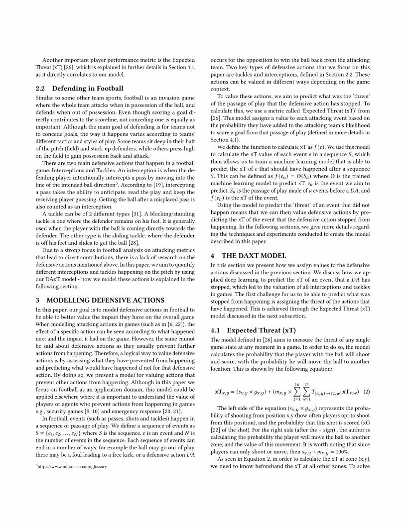
To illustrate an example, Figure 2 shows a passage of play byManchester United in a game with the xT of each action shown.The first pass (1 to 2) and dribble (2 to 3) have negative xT valuesince they are moving away from goal, decreasing the probability ofthe attacking team to score. However, the successful pass of AlexisSanchez into the penalty box resulted in a large positive xT value,indicating the increased threat of scoring a goal.

Figure 2: Passage of play showing xT of each action

In the next subsection we look at how we can use xT to traina model that can predict what would happen after a sequence ofevents.

4.2 Predicting What Was StoppedDue to its generalization mechanism [13], and application to largesets of data (such as game events), we built a simple neural networkmodel to predict the future xT of the events. Specifically, we havebuilt a Multi Layer Perceptron [30] model using the Keras4 library.As explained in Section 3,Θ is fed as input a fixed number of actions𝑆𝑎 in a passage of play (Section 5.1 shows the experiment done todetermine the number of actions 𝑎), and as output the xT of theaction after this passage of play. Table 1 shows an example of oneinput instance 𝑆𝑎 with 𝑎 = 3. Each event 𝑒 in 𝑆𝑎 is represented byits xT (𝑓 (𝑒)) and x,y coordinates. The output in this case would be“xT4", signaling the xT of the action after this passage of play.

Due to the distribution of the target values being mainly Lapla-cian with few outliers (explained further in Section 5.3), the net-work was trained using a Mean Absolute Error (MAE) loss function,shown in Equation 3.4https://keras.io

Table 1: Input example for our Neural Network model

xT1 x1 y1 xT2 x2 y2 xT3 x3 y3

𝑀𝐴𝐸 =1𝑛

𝑛∑︁𝑡=1

|𝑦𝑡 − 𝑦𝑡 | (3)

where n is the number of data points used, 𝑦𝑡 is the predictedxT for a specific instance, and 𝑦𝑡 is the actual xT for this instance.

We generate and use three main datasets. The first was formedby collecting all sequences 𝑆𝑎 (of 𝑎 consecutive actions) where eachsequence precedes a successful event 𝑒 such that 𝑒 ≠ 𝐷𝐴. Theseinstances (example in Table 1) are used as input for Θ, with the xTof the following event as output. All training and testing (random80-20 split) of Θ will be done on this dataset. The other two weremade up of valid passages of play 𝑆𝑎 that came before failed eventsthat were interrupted by a 𝐷𝐴 (one dataset for interceptions andone for tackles). After validating Θ, it will be fed as input thesedatasets to predict 𝑓 (𝑒𝑛) (equation in Section 3) i.e to predict thexT of event 𝑒𝑛 that would have happened without the 𝐷𝐴. This xToutput would thus be the valuation of each interception and tackle.

In the next subsection we discuss how we assign value to eachevent as well as to the ability of an individual player in a givengame for interceptions, tackles, and overall score.

4.3 Assigning Value to EventsAs previously mentioned, we apply our DAxT model on the 2 de-fensive action datasets to predict the xT of the event that wasinterrupted by a 𝐷𝐴. After having each interception and tackleassigned its corresponding Interception value 𝐼𝑉 and Tackle value𝑇𝑉 , we grouped these defensive actions according to the playercommitting them. We then calculated the total 𝐼𝑉 and 𝑇𝑉 for eachplayer by summing all values together and also computed the aver-age for each per interception and tackle respectively. The resultsare shown in Section 6.

Moreover, we used these metrics to deduce an overall defenderscore. In total, four features were used to obtain the score: 𝐼𝑉 , 𝑇𝑉 ,Clearance xT, and Pass xT. We combined the two metrics we gotfrom the DAxT model with the latter two to derive a final score.Clearance xT is the expected threat of a clearance5 committed bya defender. The advantage of clearances is that they are movingactions (unlike interceptions and tackles), thus have an xT valuewhich correlates to the DAxT calculated. The final feature is PassxT, which considers the expected threat of each pass committedby a defender. This feature was used to value the importance ofdefenders from an attack perspective in build up play, as this isbecoming increasingly important at the top levels.

We used the cumulative values of each feature for each player,and normalized them to a score between 0-100. When simply cal-culating the average score of the four features, the rankings weretopped by defensive-minded players. This is why we introducedweights to the equation. We applied the weights in such a waywhere the impact of defensive values will be equal to the impact ofoffensive values. This can be seen in the following equation:

5When a player kicks the ball away from their own goal [1].

𝑆𝑐 = ((𝐼𝑉 +𝑇𝑉 +𝐶𝑥𝑇 ) ÷ 3 + 𝑃𝑥𝑇 ) ÷ 4 (4)where 𝑆𝑐 is the final defender score, 𝐶𝑥𝑇 is the Clearance xT,

and 𝑃𝑥𝑇 is the Pass xT. The division by 3 was done in order toget the mean of the defensive values and the whole equation wasdivided by 4 to get the average of all values. Section 7.1 illustratesand analyzes the real-world results.

5 EMPIRICAL EVALUATIONTo evaluate and optimise our models, we used a dataset collectedfrom two seasons (2017/18 and 2018/19) from the English PremierLeague (EPL).6 The dataset breaks down each of the games fromthe tournament into an event-by-event analysis where each eventgives different metrics including: event type (e.g., pass, shot, tackleetc.), the pitch coordinates of the event and the event outcome. Thisis a rich real-world dataset that allows us to rigorously assess thevalue of our model. The experiments7 performed are as follows:

5.1 Experiment 1: Setting the ModelParameters

First, to test the model generalisation, we separated our data intotraining and validation sets (random split of 80-20). The experimentswere then ran on both sets and the MAE (Equation 3) was the metricused.

We ran an experiment to determine the number of actions 𝑎that should be taken into consideration in 𝑆𝑎 . There could be anargument about using 𝑎 = 1, since having the xT and location ofan event could be enough “threat" evidence. Another argumentwould be that using more actions would be beneficial to our modelsince it is learning more details about the passages of play. Table 2shows the training and validation losses, amount of training data,and number of each 𝐷𝐴 with different number of previous actions.

Table 2: MAE and instances for different number of actions

𝑎 = 1 𝑎 = 2 𝑎 = 3

Training Loss 0.0174 0.0154 0.0123Validation Loss 0.0169 0.0153 0.012Training Data 950,139 802,046 686,529Interceptions 98,235 75,691 59,593

Tackles 22,124 17,423 13,676

The number of training data and defensive actions availabledecreases as 𝑎 increases. This is logical, since finding 3 consecutive,successful, and moving actions in the dataset is harder than finding2 or even 1. Thus, this leads to having less available defensiveactions to value as the passages of play become longer.

As highlighted in the table, we chose 𝑎 = 2 as the optimal numberof actions for passages of play. This result was selected to balancebetween minimizing the loss of the model and maximizing thenumber of defensive actions being valued. Although their numberwas decreasing, not valuing these 𝐷𝐴 was worth the increase inaccuracy. This is due to the fact that by choosing 2 actions instead6All data provided by StatsBomb - www.statsbomb.com.7Experiments have been run using Keras and TensorFlow.

of 1, we minimized the randomness of having only 𝑎 = 1 in 𝑆𝑎(which could be considered as outliers that confuse the model),thus allowing better and more accurate sequences to be considered.This decrease in 𝐷𝐴 eliminated the repeated actions that occur insome games, with actions happening quickly after one another thatwould not interpret a defender’s true ability.

5.2 Experiment 2: Selecting the FeaturesAnother experiment was conducted in order to test different featuresets for our model. According to [2], most existing models thatanalyze football event data only use location and action type. Sinceour action type is constant, we tested different combinations offeatures that include body part, time of game and team ID, otherthan the already mentioned xT and location.

After testing different combinations, the results showed that xTand x,y coordinates were truly the most important features. Theomission of either one of them (or both) resulted in an increase inMAE > 0.002, whereas trying both features with others resulted indifferences of ≈ 0.001. The best model according to the lowest MAEvalue and best learning curve was the model that uses both of thesefeatures alone. Adding other variables was either overfitting themodel (team ID), which was expected since it disturbs the initialtactical interpretation, or was too general to make a difference(body part, where the large majority of actions was with foot).

5.3 Experiment 3: Model PredictionThe first step towards validating our model is by checking whetherits predictive performance deteriorates when applied to unseendata. When exercised on the test set, the model returned an MAEloss of 0.016, which is an accepted result according to the trainingand validation loss functions in Section 5.1.8

The first statistical test we performed was comparing the residu-als of the training and testing datasets. The residuals (errors) are thedifferences between the actual and predicted values of the model.To make sure our model does not over fit to our training data, weused the Levene test [24] and Kolmogorov-Smirnov (KS) [16] teston both residuals. These tests are conducted to compare the vari-ance (Levene) and probability distribution (KS) of our training andtesting residuals, which are expected to be similar for our modelto be considered a good fit. The Levene test returned a statisticvalue 𝑣 = 1.209 and a p-value 𝑝 = 0.272. Since the p-value is greaterthan our 5% threshold, we can then conclude that there is evidencethat both residuals have the same variance. Similarly, the KS test’sreturn of 𝑣 = 0.0174 and 𝑝 = 0.8333 > 0.05 suggests that the twoprobability distributions are the same.

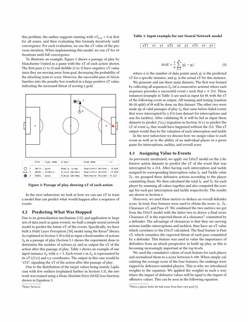
When sketching the fitted line of the probability plot (also knownas Q-Q plot [12]) in Figure 3, we could see that the residual’s dis-tribution is somewhat normal with long tails on both sides. Byvisualizing the predictions yielded by our model and comparingthem to the actual values, we observed that 96.1% of the data wasbetween 0.05 and -0.05, explaining the tails in the plot. This reason-ing was logical since actions with very high xT (or very low) rarelyhappen in games compared to regular, less significant actions.

8For comparative purposes a baseline model predicting 0’s would have a MAE of0.0267.

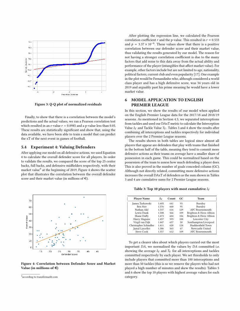
Figure 3: Q-Q plot of normalized residuals

Finally, to show that there is a correlation between the model’spredictions and the actual values, we ran a Pearson correlation testwhich resulted in an r-value 𝑟 = 0.0985 and a p-value less than 0.05.These results are statistically significant and show that, using thedata available, we have been able to train a model that can predictthe xT of the next event in games of football.

5.4 Experiment 4: Valuing DefendersAfter applying our model on all defensive actions, we used Equation4 to calculate the overall defender score for all players. In orderto validate the results, we compared the score of the top 25 centerbacks, full backs, and defensive midfielders respectively, with theirmarket value9 at the beginning of 2019. Figure 4 shows the scatterplot that illustrates the correlation between the overall defenderscore and their market value (in millions of e).

Figure 4: Correlation between Defender Score and MarketValue (in millions of e)

9according to transfermarkt.com

After plotting the regression line, we calculated the Pearsoncorrelation coefficient 𝑟 and the p-value. This resulted in 𝑟 = 0.533and 𝑝 = 3.37 × 10−6. These values show that there is a positivecorrelation between our defender score and their market value,thus validating the results generated by our model. The reason fornot having a stronger correlation coefficient is due to the manyfactors that add noise to this data away from the actual ability andperformance of the player (intangibles that affect market value). Forexample, other factors include but are not limited to age, nationality,political factors, current club and even popularity [17]. One examplein the plot would be Fernandinho who, although considered a worldclass player and has a high defensive score, was 34 years old in2019 and arguably past his prime meaning he would have a lowermarket value.

6 MODEL APPLICATION TO ENGLISHPREMIER LEAGUE

In this section, we show the results of our model when appliedon the English Premier League data for the 2017/18 and 2018/19seasons. As mentioned in Section 4.3, we separated interceptionsfrom tackles and used our DAxTmetric to calculate the InterceptionValue 𝐼𝑉 and Tackle Value 𝑇𝑉 . Tables 3 and 4 show the results aftercombining all interceptions and tackles respectively for individualplayers over the 2 Premier League seasons.

The results shown in both tables are logical since almost allplayers that appear are defenders that play with teams that finishedin the bottom half of the table, meaning they tend to commit moredefensive actions as their teams on average have a smaller share ofpossession in each game. This could be normalized based on thepossession of the team to assess how much defending a player does.This is also proved in the number of goals conceded column (GC).Although not directly related, committing more defensive actionsincreases the overall DAxT of defenders as the sum shown in Tables3 and 4 are cumulative sums for 2 Premier League seasons.

Table 3: Top 10 players with most cumulative 𝐼𝑉

Player Name 𝑰𝑽 Count GC Team

James Tarkowski 1.605 641 93 BurnleyBen Mee 1.576 660 95 Burnley

Nathan Aké 1.537 616 129 AFC BournemouthLewis Dunk 1.508 566 109 Brighton & Hove AlbionShane Duffy 1.473 604 106 Brighton & Hove Albion

Harry Maguire 1.457 593 100 Leicester CityVirgil van Dijk 1.447 657 50 Southampton/Liverpool

Christopher Schindler 1.411 620 124 Huddersfield TownJamal Lascelles 1.386 565 67 Newcastle UnitedSteve Cook 1.357 612 109 AFC Bournemouth

To get a clearer idea about which players carried out the mostimportant 𝐷𝐴, we normalized the values by 𝐷𝐴 committed i.e.showing the average 𝐼𝑉 and 𝑇𝑉 for all interceptions and tacklescommitted respectively by each player. We set thresholds to onlyinclude players that committed more than 100 interceptions andmore than 50 tackles (this is so we remove the players who had notplayed a high number of minutes and skew the results). Tables 5and 6 show the top 10 players with highest average values for eachcategory.

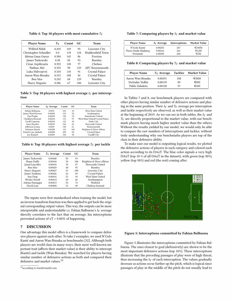
Table 4: Top 10 players with most cumulative 𝑇𝑉

Player Name 𝑻𝑽 Count GC Team

Wilfred Ndidi 0.435 169 95 Leicester CityChristopher Schindler 0.4 118 124 Huddersfield TownIdrissa Gana Gueye 0.384 142 86 EvertonJames Tarkowski 0.38 85 93 BurnleyCésar Azpilicueta 0.353 120 77 Chelsea

Nathan Aké 0.335 90 129 AFC BournemouthLuka Milivojević 0.318 110 91 Crystal Palace

Aaron Wan-Bissaka 0.315 108 56 Crystal PalaceBen Mee 0.292 68 129 Burnley

Harry Maguire 0.286 67 100 Leicester City

Table 5: Top 10 players with highest average 𝐼𝑉 per intercep-tion

Player Name 𝑰𝑽 Average Count GC Team

Fabián Balbuena 0.0031 232 32 West Ham UnitedJames Ward-Prowse 0.00306 125 92 Southampton

Paul Pogba 0.00305 138 70 Manchester UnitedCheikhou Kouyaté 0.00294 176 97 West Ham United/Crystal PalaceGeoff Cameron 0.00294 122 30 Stoke CityIsaac Hayden 0.00291 162 65 Newcastle UnitedJefferson Lerma 0.0029 140 61 BournemouthSolomon March 0.00288 125 106 Brighton & Hove Albion

Patrick van Aanholt 0.00288 289 84 Crystal PalaceJoe Bennett 0.00287 168 50 Cardiff City

Table 6: Top 10 players with highest average 𝑇𝑉 per tackle

Player Name 𝑻𝑽 Average Count GC Team

James Tarkowski 0.00448 85 93 BurnleyShane Duffy 0.00444 54 106 Brighton & Hove Albion

Jamal Lascelles 0.00443 53 67 Newcastle UnitedBen Mee 0.00429 68 95 Burnley

Harry Maguire 0.00427 67 100 Leicester CityJames Tomkins 0.00426 62 69 Crystal Palace

Issa Diop 0.00416 51 43 West Ham UnitedWesley Hoedt 0.00414 69 66 Southampton

Adrian Mariappa 0.00413 53 74 WatfordDavid Luiz 0.00404 51 49 Chelsea/Arsenal

The inputs were first standardized when training the model, butan inverse transform function was then applied to get back the origi-nal corresponding output values. This way, the outputs can be moreinterpretable and understandable i.e. Fabian Balbuena’s 𝐼𝑉 averagedirectly correlates to the fact that on average, his interceptionsprevented actions of xT = 0.0031 of happening.

7 DISCUSSIONOne advantage this model offers is a framework to compare defen-sive players against each other. To take 2 examples, we used N’GoloKanté and Aaron Wan-Bissaka as benchmarks [32]. Although bothplayers are world class in many ways, their most well-known im-portant trait (affects their market value) is their ability to intercept(Kanté) and tackle (Wan-Bissaka). We searched for players havingsimilar number of defensive actions as both and compared theirdefensive and market values.10

10according to transfermarkt.com

Table 7: Comparing players by 𝐼𝑉 and market value

Player Name 𝑰𝑽 Average Interceptions Market Value

N’Golo Kanté 0.00255 247 e100MPierre-Emile Højbjerg 0.00216 241 e12M

Fernando 0.00205 264 e5M

Table 8: Comparing players by 𝑇𝑉 and market value

Player Name 𝑻𝑽 Average Tackles Market Value

Aaron Wan-Bissaka 0.00291 108 e30MDeAndre Yedlin 0.00139 89 e8MPablo Zabaleta 0.00128 97 e4M

In Tables 7 and 8, our benchmark players are compared withother players having similar number of defensive actions and play-ing in the same position. Their 𝐼𝑉 and 𝑇𝑉 average per interceptionand tackle respectively are observed, as well as their market valueat the beginning of 2019. As we can see in both tables, the 𝐼𝑉 and𝑇𝑉 are directly proportional to the market value, with our bench-mark players having much higher market value than the others.Without the results yielded by our model, we would only be ableto compare the raw numbers of interceptions and tackles, withouttruly understanding why our benchmarks players are top of theclass in their defensive ability.

To make sure our model is outputting logical results, we plottedthe defensive actions of players in each category and colored eachaction according to its DAxT. The blue color signals a very highDAxT (top 10 % of all DAxT in the dataset), with green (top 30%),yellow (top 50%) and red (the rest) coming after.

Figure 5: Interceptions committed by Fabian Balbuena

Figure 5 illustrates the interceptions committed by Fabian Bal-buena. The ones closest to goal (defensively) are shown to be themost important defensive actions (top 10%). These interceptionsillustrate that the preceding passages of play were of high threat,thus increasing the 𝐼𝑉 of each interception. The values graduallydecrease as actions occur further up the pitch, which is logical sincepassages of play in the middle of the pitch do not usually lead to

Figure 6: Tackles committed by Andrew Robertson

conceding goals. The same concept applies to Figure 6, that illus-trates the tackles committed by Robertson. The ones which directlyled to stopping actions of high threat are in blue, and most of thetackles are on the left side of the pitch due to Robertson’s positionas a left back.

7.1 Overall Defender ScoreWe applied the overall defender score (introduced in Section 4.3) forranking and filtered out according to position (center back or fullback). We then used CIES Football Observatory and InStat Perfor-mance Index [8] for the 2019 season as a means of comparison forour rankings (CIES). Moreover, we calculated the number of goalsconceded (GC), appearances (A), goals conceded per appearance(GC/A), and assists (AST) for full backs. Table 9 shows our rankingsfor center backs while Table 10 shows the rankings for full backs.

Table 9: Ranking Center Backs according to defender score

Player Name Score GC A GC/A Rank CIES

Virgil Van Dijk 37.901 50 64 0.781 1 1Harry Maguire 36.3 100 69 1.449 2 4

Ben Mee 35.942 95 67 1.418 3 37James Tarkowski 34.733 93 66 1.409 4 13Shkodran Mustafi 34.636 70 58 1.207 5 20Jan Vertonghen 34.426 54 58 0.931 6 20

Toby Alderweireld 33.459 44 48 0.916 7 11Aymeric Laporte 33.284 26 44 0.591 8 6Nathan Aké 33.25 129 76 1.697 9 31

Michael Keane 31.913 85 63 1.349 10 37Lewis Dunk 30.572 109 74 1.472 11 26David Luiz 30.536 49 46 1.065 12 20

Antonio Rüdiger 29.975 57 60 0.95 13 17Shane Duffy 28.295 106 72 1.472 14 20

Nicolas Otamendi 27.826 32 52 0.615 15 17

Although there is a season difference between the rankings, wecan see many similarities in player standings. Most of the playersmentioned are found in both studies, assuring that our results arelogical. Moreover, our findingsmatch the top defenders identified by

Table 10: Ranking Full Backs according to defender score

Player Name Score GC A GC/A AST Rank CIES

César Azpilicueta 47.823 77 75 1.026 11 1 6Andrew Robertson 40.047 38 58 0.655 16 2 2Patrick van Aanholt 38.568 84 64 1.3125 3 3 24

Kyle Walker 31.464 39 65 0.6 7 4 12Trent Alexander-Arnold 31.31 32 48 0.66 13 5 5

Kieran Trippier 31.082 44 51 0.86 8 6 N/ARyan Bertrand 27.206 91 59 1.54 4 7 27Pablo Zabaleta 26.69 97 63 1.54 2 8 N/ABen Davies 26.44 46 56 0.82 6 9 24

Marcos Alonso 24.691 58 64 0.906 6 10 1Ben Chilwell 24.442 73 60 1.216 6 11 8

Aaron Wan-Bissaka 23.331 56 42 1.33 3 12 9Ricardo Pereira 23.046 45 35 1.285 6 13 4Luke Shaw 22.994 41 40 1.025 4 14 13

Cédric Soares 22.73 75 50 1.5 5 15 19

experts in the press for that season11. This indicates the importanceof applying statistical models such as our metrics and xT, ratherthan using raw data.

Furthermore, the tables illustrate consistency between our de-fender score and the other variables. For example, we can seethat 5 of our top 6 full backs have a low average of goals con-ceded/appearance with a high number of assists relative to the rest.Also, although Harry Maguire and Nathan Aké, for instance, havea high number of goals conceded/appearance due to the teams theywere playing for, their transfer fees (transfermarkt.com) of e87Mto Manchester United and e45M to Manchester City respectivelyshow why they are top of our ranking.

As different teams have different playing styles, valuing defend-ers as such has many advantages. Other than using it directly tocompare between players, scouts and teams could use the samemetrics but change the weights according to their needs. Instead ofequally weighing the defensive and attacking side of players, someteams (such as relegation-threatened ones) could want to focusmore on specific defensive metrics, weighing each one accordingly.Moreover, the same defender score could also be used for defen-sive midfielders. Table 11 shows the top 10 defensive midfieldersaccording to score.

Table 11: Ranking Defensive Midfielders according to de-fender score

Rank Player Name Score

1 Granit Xhaka 37.6482 Fernandinho 37.4373 Nemanja Matić 30.7374 Jorginho 27.6525 Luka Milivojević 27.2996 Abdoulaye Doucouré 25.7347 Idrissa Gueye 24.6338 Oriol Romeu 24.6299 Mark Noble 23.19710 Wilfred Ndidi 23.107

11https://www.mirror.co.uk/sport/football/news/top-10-central-defenders-premier-13772574

7.2 Remaining ChallengesOne limitation of our DAxT model is that some defensive actionswill be valued less than they should be due to unique passages ofplays. For instance, the opposition could counterattack and be in a3vs1 situation (3 players attacking while only 1 is defending) in themiddle of the pitch. If the defender intercepts the ball, our modelwould not highly reward this action because similar passages of playare not usually of high threat (without taking into considerationthe number of defenders behind the ball). This is why future workfor valuing defenders’ contributions should be centered aroundthe growing collection of tracking data. This will allow analysts toassess the off-ball contributions and movement of defenders withmodels such as pitch control [27], evaluations of oppositionmarkingand stopping events before they have happened. However, due tothe low availability of tracking data at this time, especially acrossdifferent leagues, it is key to have methods that allow defensiveactions to be valued from event-data in smarter ways.

A further challenge ourmodel faces is the dependency on anotherplayer metric. This becomes a problem in terms of interpretation,where people need to understand Expected Threat first in orderto comprehend our DAxT model. Moreover, metrics such as Pos-session Adjusted Interceptions and True Tackle Win % are slightlymore intuitive than our ratings, which complicates the task foranalytically less inclined scouts to fully grasp our model.

8 CONCLUSIONEven though the results have illustrated that our model works well,comparing it to other baseline models remains difficult due to thelack of similar work. One analogous paper is [29], where the authorsmake use of tracking data to understand the defensive impact ofplayers.

In conclusion, we have presented a novel model for valuingdefensive actions by using deep learning to predict a future eventthat a defensive action has stopped. We have introduced a newmetric DAxT by focusing on the values of tackles and interceptionsmade by defenders. This can help clubs to better understand thecontribution of defenders and identify new talent for recruitmentin the over 100 leagues that event-data is collected for.

REFERENCES[1] Alvin Almazov. [n.d.]. Clearances. http://alvin-almazov.com/soccer-eng/

clearance/[2] Daniel Altman. 2015. Beyond Shots: A New Approach to Quantifying Scoring

Opportunities. In OptaPro Analytics Forum.[3] Ryan Beal, Georgios Chalkiadakis, Timothy J Norman, and Sarvapali D Ram-

churn. 2020. Optimising Game Tactics for Football. International Conference onAutonomous Agents and Multiagent Systems (2020).

[4] Ryan Beal, Timothy J Norman, and Sarvapali D Ramchurn. 2019. Artificialintelligence for team sports: a survey. The Knowledge Engineering Review 34(2019).

[5] Benjamin Cronin. [n.d.]. An analysis of different expected goals mod-els. https://www.pinnacle.com/en/betting-articles/Soccer/expected-goals-model-analysis/MEP2N9VMG5CTW99D

[6] Tom Decroos, Lotte Bransen, Jan Van Haaren, and Jesse Davis. 2019. Actionsspeak louder than goals: Valuing player actions in soccer. In Proceedings of the 25thACM SIGKDD International Conference on Knowledge Discovery & Data Mining.1851–1861.

[7] Javier Fernández, Luke Bornn, and Dan Cervone. 2019. Decomposing the Immea-surable Sport: A deep learning expected possession value framework for soccer.In 13 th Annual MIT Sloan Sports Analytics Conference.

[8] CIES Football and InStat. [n.d.]. CIES Football Observatory and InStat PerformanceIndex. https://football-observatory.com/IMG/sites/instatindex/

[9] Jens Grossklags, Nicolas Christin, and John Chuang. 2008. Secure or insure? Agame-theoretic analysis of information security games. In Proceedings of the 17thinternational conference on World Wide Web. 209–218.

[10] Christopher Kiekintveld, Manish Jain, Jason Tsai, James Pita, Fernando Ordóñez,and Milind Tambe. 2009. Computing optimal randomized resource allocationsfor massive security games. In Proceedings of The 8th International Conference onAutonomous Agents and Multiagent Systems-Volume 1. 689–696.

[11] Gunjan Kumar. 2013. Machine learning for soccer analytics. University of Leuven(2013).

[12] Usha A Kumar. 2005. Comparison of neural networks and regression analysis: Anew insight. Expert Systems with Applications 29, 2 (2005), 424–430.

[13] Steve Lawrence, C Lee Giles, and Ah Chung Tsoi. 1998. What size neural networkgives optimal generalization? Convergence properties of backpropagation. TechnicalReport.

[14] Wen-Yau Liang, Chun-Che Huang, Tzu-Liang Bill Tseng, Yin-Chen Lin, andJuotzu Tseng. 2012. The evaluation of intelligent agent performance—an exampleof B2C e-commerce negotiation. Computer Standards & Interfaces 34, 5 (2012),439–446.

[15] Patrick Lucey, Alina Bialkowski, Mathew Monfort, Peter Carr, and Iain Matthews.2014. quality vs quantity: Improved shot prediction in soccer using strategicfeatures from spatiotemporal data. In Proc. 8th annual mit sloan sports analyticsconference. 1–9.

[16] Frank J Massey Jr. 1951. The Kolmogorov-Smirnov test for goodness of fit. Journalof the American statistical Association 46, 253 (1951), 68–78.

[17] Oliver Müller, Alexander Simons, and Markus Weinmann. 2017. Beyond crowdjudgments: Data-driven estimation of market value in association football. Euro-pean Journal of Operational Research 263, 2 (2017), 611–624.

[18] Thomy Phan, Lenz Belzner, Thomas Gabor, and Kyrill Schmid. 2018. Leveragingstatistical multi-agent online planning with emergent value function approxima-tion. arXiv preprint arXiv:1804.06311 (2018).

[19] Dick’s pro tips. [n.d.]. Defensive Soccer Skills: Anticipating & Intercepting thePass with Becky Sauerbrunn. https://protips.dickssportinggoods.com/sports-and-activities/soccer/defensive-soccer-skills-anticipating-intercepting-pass

[20] Sarvapali D Ramchurn, Trung DongHuynh, Yuki Ikuno, Jack Flann, FengWu, LucMoreau, Nicholas R Jennings, Joel E Fischer, Wenchao Jiang, Tom Rodden, et al.2015. HAC-ER: A disaster response system based on human-agent collectives.In Proceedings of the 14th International Conference on Autonomous Agents andMulti-Agent Systems (AAMAS). 533–541.

[21] Sarvapali D Ramchurn, Feng Wu, Wenchao Jiang, Joel E Fischer, Steve Reece,Stephen Roberts, Tom Rodden, Chris Greenhalgh, and Nicholas R Jennings. 2016.Human–agent collaboration for disaster response. Autonomous Agents and Multi-Agent Systems 30, 1 (2016), 82–111.

[22] Alex Rathke. 2017. An examination of expected goals and shot efficiency insoccer. Journal of Human Sport and Exercise 12, 2 (2017), 514–529.

[23] Oliver Schulte, Mahmoud Khademi, Sajjad Gholami, Zeyu Zhao, Mehrsan Javan,and Philippe Desaulniers. 2017. A Markov Game model for valuing actions,locations, and team performance in ice hockey. Data Mining and KnowledgeDiscovery 31, 6 (2017), 1735–1757.

[24] Brian B Schultz. 1985. Levene’s test for relative variation. Systematic Zoology 34,4 (1985), 449–456.

[25] Eric Shieh, Bo An, Rong Yang, Milind Tambe, Craig Baldwin, Joseph DiRenzo,Ben Maule, and Garrett Meyer. 2012. PROTECT: An application of computationalgame theory for the security of the ports of the United States. In Proceedings ofthe AAAI Conference on Artificial Intelligence, Vol. 26.

[26] Karun Singh. [n.d.]. Introducing Expected Threat (xT). https://karun.in/blog/expected-threat.html

[27] William Spearman. 2018. Beyond expected goals. In Proceedings of the 12th MITsloan sports analytics conference. 1–17.

[28] SPIFFYD. [n.d.]. Soccer Tackling Techniques: Types of Tackles. https://howtheyplay.com/team-sports/Soccer-tackling-techniques-Types-of-tackles

[29] Michael Stöckl, Thomas Seidl, Daniel Marley, and Paul Power. [n.d.]. MakingOffensive Play Predictable-Using a Graph Convolutional Network to UnderstandDefensive Performance in Soccer. ([n. d.]).

[30] Jiexiong Tang, Chenwei Deng, and Guang-Bin Huang. 2015. Extreme learningmachine for multilayer perceptron. IEEE transactions on neural networks andlearning systems 27, 4 (2015), 809–821.

[31] Lim Weiyang. [n.d.]. How do you tackle in football? https://www.myactivesg.com/Sports/Football/Training-Methods/Football-for-Beginners/How-to-tackle-in-football#:~:text=There%20are%202%20types%20of,known%20as%20the%20sliding%20tackle.

[32] Tom Worville. [n.d.]. Underlying stats stars of 2020: Giroud, Lloris, Buendia, Rice –and Leeds. https://theathletic.com/2280965/2020/12/31/analytics-review-giroud-lloris-rice-leeds/

A APPENDIX ON REPRODUCIBILITYIn this appendix we give further details on our models and tech-niques used for reproducibility purposes.

A.1 Data ConversionFor this project, we used StatsBomb’s event-based data for the2017/2018 and 2018/2019 English Premier League seasons (total of760 games). Due to the inconsistency of events in terms of number offeatures, we used a data abstraction package called SPADL (SoccerPlayer Action Description Language). As mentioned in [6], SPADLtransforms the event stream data of JSON format into “a commonvocabulary that enables subsequent data analysis." This librarywas created to convert different data providers’ event data into aconsistent format. Therefore, our model is reproducible with anydata. Table 12 shows some features of the first 5 instances in theevent-stream data.

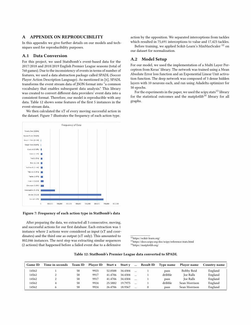
We then calculated the xT of every moving successful action inthe dataset. Figure 7 illustrates the frequency of each action type.

Figure 7: Frequency of each action type in StatBomb’s data

After preparing the data, we extracted all 3 consecutive, moving,and successful actions for our first database. Each extraction was 1instance where 2 actions were considered as input (xT and coor-dinates) and the third one as output (xT only). This amounted to802,046 instances. The next step was extracting similar sequences(2 actions) that happened before a failed event due to a defensive

action by the opposition. We separated interceptions from tackleswhich resulted in 75,691 interceptions to value and 17,423 tackles.

Before training, we applied Scikit-Learn’s MinMaxScaler 12 onour dataset for normalization.

A.2 Model SetupFor our model, we used the implementation of a Multi Layer Per-ceptron from Keras’ library. The network was trained using a MeanAbsolute Error loss function and an Exponential Linear Unit activa-tion function. The deep network was composed of 3 dense hiddenlayers with 10 neurons each, and ran using Adadelta optimizer for50 epochs.

For the experiments in the paper, we used the scipy.stats13 libraryfor the statistical outcomes and the matplotlib14 library for allgraphs.

12https://scikit-learn.org/13https://docs.scipy.org/doc/scipy/reference/stats.html14https://matplotlib.org/

Table 12: StatBomb’s Premier League data converted to SPADL

Game ID Time in seconds Team ID Player ID Start x Start y ... Result ID Type name Player name Country name

14562 1 58 9923 52.0588 34.4304 ... 1 pass Bobby Reid England14562 2 58 9917 41.4706 34.4304 ... 1 dribble Joe Ralls England14562 2 58 9917 41.4706 34.4304 ... 1 pass Joe Ralls England14562 4 58 9924 25.5882 19.7975 ... 1 dribble Sean Morrison England14562 6 58 9924 26.4706 18.9367 ... 0 pass Sean Morrison England