What Drives Changes in Carbon Emissions? An Index ...

Dis cus si on Paper No. 14-038

What Drives Changes in Carbon Emissions?

An Index Decomposition Approach for 40 Countries

Michael Schymura and Sebastian Voigt

Dis cus si on Paper No. 14-038

What Drives Changes in Carbon Emissions?

An Index Decomposition Approach for 40 Countries

Michael Schymura and Sebastian Voigt

Download this ZEW Discussion Paper from our ftp server:

http://ftp.zew.de/pub/zew-docs/dp/dp14038.pdf

Die Dis cus si on Pape rs die nen einer mög lichst schnel len Ver brei tung von neue ren For schungs arbei ten des ZEW. Die Bei trä ge lie gen in allei ni ger Ver ant wor tung

der Auto ren und stel len nicht not wen di ger wei se die Mei nung des ZEW dar.

Dis cus si on Papers are inten ded to make results of ZEW research prompt ly avai la ble to other eco no mists in order to encou ra ge dis cus si on and sug gesti ons for revi si ons. The aut hors are sole ly

respon si ble for the con tents which do not neces sa ri ly repre sent the opi ni on of the ZEW.

What Drives Changes in Carbon Emissions?An Index Decomposition Approach for 40 Countries

Michael Schymura1,∗, Sebastian Voigt2

Centre for European Economic Research (ZEW), L 7, 1, D-68161, Mannheim, Germany

Abstract

This study analyzes carbon emission trends and drivers in 40 major economies using the WIOD database, a harmo-nized and consistent dataset of input-output table time series accompanied by environmental satellite data. We uselogarithmic mean Divisia index decomposition to (1) study trends in global carbon emissions between 1995 and 2009,(2) attribute changes in carbon emissions to either influences of economic activity, changes in technology, changes inthe structure of the economy, alterations of the fuel mix, or changes in carbon intensities of specific fuel types, and (3)highlight sectoral and regional differences. We first find that heterogeneity in each country is higher than heterogeneityin sectors. This finding might lead to the conclusion that, in order to abate CO2, structural conditions in sectors prevailover regional circumstances. Regarding our results of the decomposition analysis, the drivers of changes in carbonemissions are very heterogeneous. Among the world’s top ten emitters, in only three countries – China, Germanyand Canada – the main driver of an improved emissions performance was technological change. Conversely, in Japanand Australia structural change of the economy contributed to less severe increases of emissions. The deploymentof cleaner energy sources had a positive in some, mainly developed, economies. Moreover, our results for the globallevel suggest a general move towards more efficient means of production.

Keywords: Carbon emissions, Logarithmic mean Divisia index decomposition, WIOD databaseJEL classification: Q43, C43

1. Introduction

Current and projected trends for population, income and energy demand growth suggest that the pressure on energyand natural resources will increase in the coming decades, especially in emerging and developing economies. Thiswill result in higher levels of anthropogenic emissions unless the world economy switches away from fossil-basedenergy carriers by facilitating access to more efficient technologies, favoring structural change in the composition ofeconomic activities or increasing the willingness to pay for a clean environment.3 An important first step to reducegreenhouse gas emissions without negatively affecting economic welfare too heavily is the reduction of their intensity,i.e. their units of emissions per output unit. In particular, the intensity of the most significant greenhouse gas CO2 isof major importance (Canadell et al., 2007, Raupach et al., 2007).

∗Corresponding author1Centre for European Economic Research (ZEW), L 7, 1, D-68161, Mannheim, Germany. Mail: [email protected], Phone: +49 (0)621

1235-202, Fax: +49 (0)621 1235-2262Centre for European Economic Research (ZEW), L 7, 1, D-68161, Mannheim, Germany. Mail: [email protected], Phone: +49 (0)621 1235-219,

Fax: +49 (0)621 1235-2263By 2050, the United Nations projects global population to be almost 9.2 billion. Growth rates are projected to be positive in BRIICS (Brazil,

Russia, India, Indonesia, China and South Africa) countries, but they are expected to be particularly high in Africa and South Asia, while populationwill fall in some European countries, Japan and Korea. Urbanization and average per capita income levels are also expected to increase (OECD,2012). The increased demographic pressure in less developed countries will have important repercussions for energy demand and use, and henceCO2 emissions will further increase. From 2010 to 2040 the US Energy Information Administration forecasts an energy-related CO2 emissiongrowth in OECD countries of 0.2% p.a., while emissions in non-OECD countries will grow by 1.9% p.a. (IEO, 2013, p. 159).

1995

1996

1997

1998

1999

2000

2001

2002

2003

2004

2005

2006

2007

2008

2009

5

10

15

20

25

CarbonEmissionsin

billiontons

EU27 (+ TUR) AUS

BRA MEX CAN CHNASIA RUSUSA

1

(a) Regional distribution in 2009

00.1

0.2

0.3

0.4

0.5

0.6

0.7

0.8

0.9 1

0

0.1

0.2

0.3

0.4

0.5

0.6

0.7

0.8

0.9

1

Cumulative population proportion

Total

CO2em

ission

s

EqualityLorentz Curve CO2 1995Lorentz Curve CO2 2009

Lorentz Curve Gross Output 1995Lorentz Curve Gross Output 2009

(b) Lorentz curves 1995 & 2009

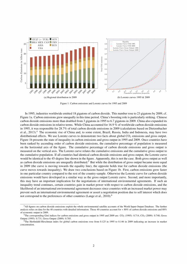
Figure 1: Carbon emissions and Lorentz curves for 1995 and 2009

In 1995, industries worldwide emitted 18 gigatons of carbon dioxide. This number rose to 23 gigatons by 2009, cf.Figure 1a. Carbon emissions grew unequally in this time period. China’s boosting role is particularly striking. Chinesecarbon dioxide emissions more than doubled from 3 gigatons in 1995 to 6.7 gigatons in 2009. China also expanded itscarbon dioxide emissions in relative terms. While China accounted for 16.9 % of worldwide carbon dioxide emissionsin 1995, it was responsible for 28.7% of total carbon dioxide emissions in 2009 (calculations based on Dietzenbacheret al., 2013).4 The economic rise of China and, to some extent, Brazil, Russia, India and Indonesia, may have twodistributional effects. We use Lorentz curves to demonstrate two facts about global CO2 emissions and gross output.Figure 1b presents the state of inequality in carbon emissions and gross output in 1995 and 2009. Once countries havebeen ranked by ascending order of carbon dioxide emissions, the cumulative percentage of population is measuredon the horizontal axis of the figure. The cumulative percentage of carbon dioxide emissions and gross output ismeasured on the vertical axis. The Lorentz curve relates the cumulative emissions and the cumulative gross output tothe cumulative population. If all countries had identical carbon dioxide emissions and gross output, the Lorentz curvewould be identical to the 45-degree line shown in the figure. Apparently, this is not the case. Both gross output as wellas carbon dioxide emissions are unequally distributed.5 But while the distribution of gross output became more equalin 2009 (the curve is moving towards the equality line), the opposite holds true for carbon dioxide emissions (thecurve moves towards inequality). We draw two conclusions based on Figure 1b. First, carbon emissions grew fasterin one particular country compared to the rest of the country-sample. Otherwise the Lorentz curve for carbon dioxideemissions would have developed in a similar way as the gross output Lorentz curve. Second, and more importantly,this may have an important implication for the negotiations of international environmental agreements. If such aninequality trend continues, certain countries gain in market power with respect to carbon dioxide emissions, and thelikelihood of an international environmental agreement decreases since countries with an increased market power mayprevent such an international environmental agreement or assert a negotiation position due to self interest which doesnot correspond to the preferences of other countries (Lange et al., 2010).6

4All figures on carbon dioxide emissions exploit the whole environmental satellite accounts of the World Input-Output Database. The furtheranalysis relies on data for the 40 countries with detailed information. Those 40 countries account for ≈ 80% of carbon dioxide emissions and 88%of economic output in 2009.

5The corresponding Gini indices for carbon emissions and gross output in 1995 and 2009 are: CO2 (1995): 0.714, CO2 (2009): 0.740, GrossOutput (1995): 0.731, Gross Output (2009): 0.705.

6The Herfindahl-Hirschman index for global carbon emissions rose from 0.125 in 1995 to 0.146 in 2009 indicating an increase in marketconcentration.

2

The evolution of carbon emissions may be attributable to several separate factors, namely changes in the structuralcomposition of the world economy, improvements in the technologies used for production worldwide, an alterationof the fuel mix and economic growth. Economies have shifted toward less carbon intensive sectors, resulting indeclining carbon intensities throughout most countries. At the same time, carbon intensity within all sectors of theworld’s economies is likely to decrease further as a result of more efficient production technologies and newer vintagesof capital equipment inducing advanced CO2 abatement options.

Understanding the drivers behind the national and sectoral dynamics of carbon emissions and the interplay ofstructural changes, altering fuel mixes and improved sectoral abatement options has therefore important policy impli-cations. It raises the following questions: Is the development of carbon emissions similar in the same sector acrossdifferent countries? Is the development on a global scale driven by changes in some economies and sectors rather thanothers? Most importantly, is the development of carbon emissions caused by changes in the economic structure from“dirty” to “cleaner” sectors or do actual technology improvements induce these reductions?

Answering these questions helps clarify if the decoupling between output and carbon emissions is attributable toincreased sectoral abatement options and better technologies. In this case, policies encouraging technology transfers,economies of scale and learning-by-doing effects can be put in place to replicate improvements in less developedregions which still display higher emissions levels. These improvements would then come at relatively low costssince required technologies are already available. This also has implications for the negotiations of internationalenvironmental agreements and the optimal policy design. If technological improvements can be replicated, the im-plementation of agreements based on technology transfer might be a better choice in terms of incentive compatibilitythan the design of new regulatory frameworks to promote the participation of developing countries (Aldy et al., 2010).

This study makes three contributions to the literature. First, we provide an overview of carbon emissions devel-opment with a temporal and geographical focus that is greater than in prior studies (Greening et al., 1998, Greening,2004). Second, by focusing on sectors and showing their performance across countries, we provide a novel perspec-tive that sheds light on the heterogeneity of sectoral carbon emissions development across countries. We also presenta more traditional country-based analysis, in which the sectoral composition of each economy is taken into account.We exploit the international dimension of the WIOD database, which covers the period between 1995 and 2009 andcontains data on 34 sectors in 40 major economies, including BRIC (Brazil, Russia, India and China) and other de-veloping countries. The economies included in our analysis represented approximately 88% of the world’s GDP and80% of carbon dioxide emissions in 2009. Third, we analyze carbon emissions developments based on index decom-position. This is to some degree an extension of the index decomposition literature which has so far mainly focused onenergy efficiency issues (Ang, 1994, Boyd and Roop, 2004, Choi and Ang, 2012, Mulder and De Groot, 2012, Voigtet al., 2014). We use logarithmic mean Divisia index decomposition analysis to disentangle five different effects andtheir relative contribution to the development of carbon dioxide emissions. We account for economic growth (activityeffect), efficiency improvements within the sectors of an economy (technology effects), structural change (structuraleffects) which accounts for the sectoral composition of the world’s economy, an altering fuel mix (fuel mix effect)and changes in the carbon content of the energy carriers (emission factor effect). Compared to most of the previousliterature on decomposition, we thus further disaggregate the technology effect. The “classical” technology effect (e.g.in a two factor decomposition) encompasses three instances, namely an improvement in the efficiency of production,changes in the composition of energy carriers, and carbon intensity changes of specific fuel types, and may hence beafflicted with an aggregation bias. Our five factor analysis disentangles these three aspects of technological progress.

We perform this exercise both at the aggregate and at the country level and provide insights into the heterogeneityof the drivers of carbon emissions developments in our sample.

The remainder of the paper is organized as follows. In section 2 we present the data used in the analysis. Section3 describes the development of carbon emissions in our sample both from the sectoral and the country perspective.Section 4 introduces the index decomposition framework and section 5 presents the result of this exercise. Section 6concludes by highlighting the main implications of our findings.

3

NACE WIOD industriesAtB Agriculture, hunting, forestry and fishingC Mining and quarrying15t16 Food , beverages and tobacco17t18 Textiles and textile products19 Leather, leather products and footwear20 Wood and products of wood and cork21t22 Pulp, paper, paper products, printing and publishing23 Coke, refined petroleum and nuclear fuel24 Chemicals and chemical products25 Rubber and plastics26 Other non-metallic mineral products27t28 Basic metals and fabricated metal products29 Machinery nec30t33 Electrical and optical equipment34t35 Transport equipment36t37 Manufacturing nec, recyclingE Electricity, gas and water supplyF Construction50 Sale, maintenance and repair of motor vehicles51 Wholesale trade and commission trade52 Retail trade, except of motor vehicles and motorcyclesH Hotels and restaurants60 Inland transport61 Water transport62 Air transport63 Supporting and auxiliary transport activities64 Post and telecommunicationsJ Financial intermediation70 Real estate activities71t74 Renting of machinery and equipment and other business activitiesL Public administration and defence, social securityM EducationN Health and social workO Other community, social and personal services

Table 1: WIOD industries and definition by NACE

2. Data Description: The WIOD Database

The main data source for our analysis is the newly released World Input-Output Database (WIOD, 2012).7 TheWIOD database is built on national accounts data which was developed within the 7th Framework Programme ofthe European Commission.8 The relevant information for the analysis of carbon emissions developments is includedin the Social Economic Accounts (SEA) and the emissions information which are accompanying satellite accountsto the WIOD database. Carbon emissions (C) are measured in physical units (kt) and are aggregated across 26energy carriers. The measure of sectoral economic activity relevant for our analysis is gross output (GO) which isexpressed in monetary units in basic 1995 prices and converted to million US$ (1995) using market exchange rates.The WIOD database has two main advantages. First, throughout the data collection effort, harmonization procedureswere applied to ensure international comparability of the basic data. This ensures data quality and minimizes therisk of measurement errors which are now rather unlikely to occur. Second, WIOD includes sectoral price deflators,the use of which allows to retain important information and the heterogeneity of the sectors with respect to pricedevelopments. This represents an improvement over the use of aggregate national price deflators. A complete list of

7The WIOD database and all satellite accounts are available at http://www.wiod.org. In this paper we use data released in April 2012.8The WIOD project has been funded by the European Commission, Research Directorate General as part of the 7th Framework Programme,

Theme 8: Socio-Economic Sciences and Humanities. Grant Agreement no: 225 281.

4

the 34 sectors that represent one of our units of observation over the period from 1995 to 2009 is presented in Table1.9

The structure of the WIOD database hence allows us to address the research questions outlined above by focusingon many heterogeneous countries over a fairly long time span. This is an improvement over the previously availableliterature which was more limited geographically and with respect to the time dimension.

3. Carbon Emissions Developments between 1995 and 2009

Before diving into the decomposition analysis, we examine some descriptive characteristics of carbon emissionsgrowth in our sample between the beginning and the end of the sample period. We first show the performance of eachsector covered in the database and then move on to the country analysis. From 1995 to 2009, aggregate CO2 emissionsof the 40 economies included in our sample increased by 28.6% (Figure 1a). Over the time period considered, wecan identify three time intervals characterized by a different pace of emissions growth: 1995 to 2002 when carbonemissions increased modestly by 9.2%, 2002 to 2007 when the rise occurred at a much higher pace, i.e. 19.2% in fiveyears, and 2007 to 2009 when emissions even declined by 1.2%.

3.1. Sectoral Developments

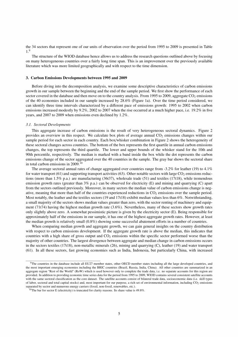
This aggregate increase of carbon emissions is the result of very heterogeneous sectoral dynamics. Figure 2provides an overview in this respect. We calculate box plots of average annual CO2 emissions changes within oursample period for each sector in each country. Each box/whisker combination in Figure 2 shows the heterogeneity ofthese sectoral changes across countries. The bottom of the box represents the first quartile in annual carbon emissionschanges, the top represents the third quartile. The lower and upper bounds of the whisker stand for the 10th and90th percentile, respectively. The median is marked with a band inside the box while the dot represents the carbonemissions change of the sector aggregated over the 40 countries in the sample. The gray bar shows the sectoral sharein total carbon emissions in 2009.10

The average sectoral annual rates of change aggregated over countries range from -3.2% for leather (19) to 4.1%for water transport (61) and supporting transport activities (63). Other notable sectors with large CO2 emissions reduc-tions (more than 1.5% p.a.) are manufacturing (36t37), wholesale trade (51) and textiles (17t18), while tremendousemission growth rates (greater than 3% p.a.) can be observed for electricity (E) and mining and quarrying (C) apartfrom the sectors outlined previously. Moreover, in many sectors the median value of carbon emissions change is neg-ative, meaning that more than half of the countries experienced reductions in CO2 emissions over the sample period.Most notably, the leather and the textiles sectors (19 and 17t18) exhibit median values less than 6%. Notwithstanding,a small majority of the sectors shows median values greater than zero, with the sector renting of machinery and equip-ment (71t74) having the highest median growth rate (3.6%). Nevertheless, many of these sectors show growth ratesonly slightly above zero. A somewhat pessimistic picture is given by the electricity sector (E). Being responsible forapproximately half of the emissions in our sample, it has one of the highest aggregate growth rates. However, at leastthe median growth is relatively small (0.8%) showing some successful abatement efforts in a number of countries.

When comparing median growth and aggregate growth, we can gain general insights on the country distributionwith respect to carbon emissions development. If the aggregate growth rate is above the median, this indicates thatcountries with a high share of gross output and CO2 emissions within the specific sector performed worse than themajority of other countries. The largest divergence between aggregate and median change in carbon emissions occursin the sectors textiles (17t18), non-metallic minerals (26), mining and quarrying (C), leather (19) and water transport(61). In all these sectors, fast growing economies such as India, Indonesia, but particularly China, with increased

9The countries in the database include all EU27 member states, other OECD member states including all the large developed countries, andthe most important emerging economies including the BRIC countries (Brazil, Russia, India, China). All other countries are summarized in anaggregate region “Rest of the World” (RoW) which is used however only to complete the trade data, i.e. no separate accounts for this region areprovided. In addition to providing economic time series data for the period from 1995 to 2009, WIOD contains several consistent satellite accountswith the same sectoral classification as the core dataset. The satellite accounts consist of bilateral trade data, socioeconomic data (i.e. skill typesof labor, sectoral and total capital stocks) and, most important for our purpose, a rich set of environmental information, including CO2 emissionsseparated by sector and numerous energy carriers (fossil, non-fossil, renewables, etc.).

10The bar for sector E (electricity) is truncated for clarity reasons. Its share value is 49.8%.

5

AtB C

15t16

17t18 19 20

21t22 23 24 25 26

27t28 29

30t33

34t35

36t37 E F 50 51 52 H 60 61 62 63 64 J 70

71t74 L M N O

−20

−17

−14

−11

−8

−5

−2

1

4

7

10

13

16

Sectoralgrow

thratesof

carbon

emissionsfrom

1995

to2009

(%)

0

5

10

15

20

25

30

35

40

45

50

Share of sectors in total carbon emissions in 2009 (%)

1

Figure 2: Annual sectoral changes in CO2 emissions. For the sector definition, see Table 1. Bottom of box represents first quartile, top representsthird quartile, band marks median. Lower and upper bounds of whisker represent 10th and 90th percentile, respectively. Dots mark carbonemissions change of the sector aggregated over the sample countries.

importance and high sectoral output and emission shares determine this finding. Especially in the non-metallic miner-als, mining and quarrying and water transport sectors, where median growth is either negative or just slightly greaterthan zero, the consequences are thus quite severe. Emissions abatement should concentrate on such countries to im-prove the global performance in these sectors. Sectoral marginal abatement costs in these countries are expected to berelatively low. This gives rise to sectoral approaches in order to achieve aggregate emissions reductions.

Conversely, some sectors show lower aggregate than median growth rates. In these cases, countries with high grossoutput and emissions shares presumably performed better than the majority. The four sectors with the largest wedgein this regard are retail trade (52), other community services (O), wholesale trade (51) and public administration anddefence (L). These results are dominated by large developed economies, above all the United States, and could hencebe replicated in emerging economies through technology transfer. However, all these sectors are service sectors witha very low share in global emissions and are thus hardly able to influence aggregate emissions reductions on a largescale.

A number of sectors perform particularly well showing reductions in carbon emissions in the vast majority of oursample countries, as the third quartile lies below or slightly above zero. These include textiles (17t18), leather (19),food, beverages and tobacco (15t16), pulp and paper (21t22), and agriculture, hunting, forestry and fishing (AtB).

Two sectors show a markedly high heterogeneity of carbon emissions changes across countries, namely the leather(19) and the mining and quarrying (C) sectors. Among the sectors with the smallest heterogeneity across countriesthree industries are particularly worth mentioning due to their relatively high share in global CO2 emissions: electricity(E), inland transport (60) and coke and refined petroleum products (23). As the former two sectors exhibit quite largeincreases during the sample period, this result may give grounds for some pessimism since there seems to be nocountry taking a strong leading role in reducing carbon emissions.

The aggregate sectoral analysis has shown that in some sectors heterogeneity of carbon emissions changes acrosscountries is high. This suggests that in these sectors there might be benefit from supporting the diffusion of efficienttechnologies from more frontier countries to the laggards. Technology diffusion and transfer could improve the overallperformance, in particular if directed toward the biggest economies in terms of gross output and CO2 emissions shares.However, in some sectors with high emissions shares, there seems to be a quite homogeneous development across theworld. Therefore, in these sectors a global effort to reduce carbon emissions might be a promising approach for asustainable improvement.

The analysis presented so far shows a mixed picture of emission reduction achievements throughout our samplesectors. In particular, the electricity sector as the world’s largest emitter shows high growth rates while the largest

6

emissions reduction occurred primarily in service sectors as well as in the textile and leather sectors. Moreover,heterogeneity can be detected in many economic branches with respect to the performance of different countries.

In the following subsection we present a similar descriptive analysis focusing on the country level before movingto the decomposition analysis.

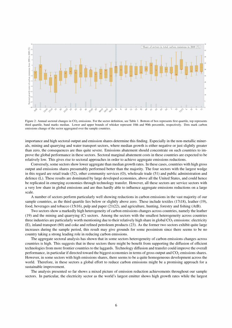
3.2. Country Level DevelopmentsWe now explore the heterogeneity of changes in carbon emissions across countries. Figure 3 shows their distri-

bution for all sectors within a given country. The box plots are constructed in a manner analogous to those shown inFigure 2. Also in this case, if the growth rate aggregated over all sectors within one country (dot) is above the median(band within box), this indicates that sectors with a high share of gross output and CO2 emissions within the specificcountry performed worse than the majority of other sectors and vice versa.

AUSAUT

BELBGRBRACANCHNCYP

CZEDEU

DNK ES

PEST

FIN

FRAGBR

GRC

HUN

IDN

IND

IRL

ITA

JPN

KOR

LTU

LUX

LVA

MEX M

LTNLD

POLPRTROU

RUSSVK

SVN

SWETURTW

NUSA

−14

−11

−8

−5

−2

1

4

7

10

13

16

Country

grow

thratesof

carbon

emissionsfrom

1995

to2009

(%)

0

4

8

12

16

20

24

28

32

Share of countries in total carbon emissions in 2009 (%)

1

Figure 3: Annual regional changes in CO2 emissions. Bottom of box represents first quartile, top represents third quartile, band marks median.Lower and upper bounds of whisker represent 10th and 90th percentile, respectively. Dots mark carbon emissions change of the country aggregatedover the sample sectors.

Similar to the sectoral analysis, we observe a mixed picture between countries that were able to reduce carbonemissions and those that increased their emissions. While the former group consists to a high extent of countries inthe former Eastern Bloc, i.e. in these cases the development may be attributed to the economic recession after thepolitical transition in 1989/1990, a large share of the latter group are emerging economies. The extent of the changescovers a broad span. The highest reduction rates are achieved in Romania (3.8% p.a.), Slovakia (2.1% p.a.) andLatvia (2.0% p.a.), whereas we observe the largest emission growth rates in China (6.2% p.a.), India (5.5% p.a.) andIndonesia (4.9% p.a.) – three of the most prominent emerging economies. The picture is heterogeneous also for thefour economies with high CO2 emissions shares, i.e. China, the US, India and Russia, where the US and Russia kepttheir emissions more or less stable when considering only the years 1995 and 2009. The results are clearly driven bythe evolution of economic growth, especially in the emerging economies. We will have a deeper look at this aspect aswell as at the country-specific temporal development in the context of our decomposition analysis in section 5.

With respect to the spread of carbon emissions changes across the sectors in each country we observe largedifferences. Some countries – namely the US, Japan, Germany, Bulgaria, Slovakia and Malta– have third quartilesbelow zero, i.e. a vast majority of the sectors actually reduced their CO2 emission levels. The opposite, i.e. the firstquartile is above zero, is true for India, Brazil, Mexico, Indonesia, Spain and Turkey. Hence, these countries exhibitnot only an aggregate emissions increase, but also the majority of sectors raised their carbon emissions.

Also in this case, we can compare median growth rates with aggregate growth rates. Contrary to the sectoral casehowever, in half of the countries the difference between both parameters is less than one, i.e. there are no significantoutlier sectors distorting the overall outcomes. Some notable counterexamples are China, Taiwan and South Koreawith aggregate above median growth rates, and Romania and Estonia with aggregate below median growth rates. In

7

the former countries mainly mining and quarrying as well as the transport sectors performed worse than most othersectors, while in the latter group heavy industrial sectors, e.g. metals, machinery and chemicals, reduced emissionstremendously – once again indicating the industrial decay in Eastern European countries after the political transition.

In comparison to the sectoral analysis presented in Figure 2, heterogeneity in the change of carbon emissions is, ingeneral, more pronounced within countries than within sectors. The average difference between the 90th and the 10thpercentile is 12.6 for countries while it is 11.0 for the sectoral perspective. This indicates that conditions in a givensector have a stronger influence on the development of carbon emissions than conditions in a given country implyinga possible similarity of sectors across the globe with respect to CO2 abatement options.

The descriptive analysis presented in this subsection shows a very heterogeneous performance in terms of carbonemissions development among our sample countries. The largest emission reductions have been achieved by East-ern European countries as well as by some Western developed economies, whereas emerging economies exhibit thehighest increases. Also the spread of change across domestic sectors is broad. We kept the descriptive analysis at thecountry level quite brief as a deeper analysis will follow in the remainder of this paper. Hence, in the next sections, wedescribe the applied decomposition approach and decompose the development of both aggregate and country carbonemission levels to show to what extent they have been due to economic growth, to shifts in the sectoral compositionof global and country production, to the improvements of the technological component, to changes in the fuel mix, orto modifications in the carbon content of the different fuel types.

4. The Mean Divisia Index Decomposition of Carbon Emissions

While the descriptive analysis presented so far is illustrative of the emissions development across sectors andcountries, it does not inform about the drivers behind the changes which have occurred. In this section, we use adecomposition analysis of carbon emissions to shed light on these issues, both at the aggregate and the country level.

The development of carbon emissions in the economy can be attributed to five different but equally relevantchanges. First, carbon emissions can increase or decline as a result of changes in the activity level of the entireeconomy (activity effect). Second, the development of carbon emissions depends on changes in the industrial activitycomposition (structural effect). Third, changes in overall carbon emissions may also result from sectoral energyintensity improvements or deteriorations (technology or intensity effect). Fourth, the composition of the fuel mixinfluences the extent of carbon emissions (fuel mix effect). And fifth, the emission factors of the specific fuel typesmay change over time and hence affect the amount of total carbon emissions (emission factor effect), e.g. switchingfrom a low to a higher quality type of gasoline.

The main purpose of this paper is to study the trends in carbon emissions in 40 economies and disentangle in de-tail the contributions from each of the above mentioned effects. Such a research question can be addressed using twobroad categories of decomposition methodologies: approaches based on input-output analysis, called structural de-composition analysis (SDA), and disaggregation techniques which can be referred to as index decomposition analysis(IDA) and which are related to index number theory in economics.11

We use an index decomposition approach (IDA) as described by Ang and Zhang (2000), Ang and Liu (2001),Boyd and Roop (2004), Ang and Liu (2007) and more recently by Choi and Ang (2012) or Su and Ang (2012) fortotal, sectoral and national energy intensities and adjust this approach to analyze carbon emissions. We focus onthe structural changes that affect the supply side of the economy (productive sectors) and thus exclude the privatehouseholds.

Following Ang and Zhang (2000), we rely on multiplicative decomposition and use the logarithmic mean Divisiaindex (LMDI-I) approach (Ang and Choi, 1997). This methodology offers very important advantages: (1) it is zero-value robust (Ang et al., 1998, p. 491) and (2) it “yields perfect decomposition” (Ang et al., 1998, p. 495), i.e. nounexplained residual exists. The latter is a considerable advantage with respect to the arithmetic mean Divisia index

11The roots of index numbers can be traced back to the French Dutot in 1738 and the Italian Carli in 1764 (Chance, 1966, Diewert, 1993).See also Diewert (1993) for a technical summary of index number theory. Boyd and Roop (2004) offer a more comprehensive review of differentindices in the context of energy intensity and the index number problem in economics. The SDA and IDA are not the only approaches for analyzingenergy intensity trends. Kim and Kim (2012), for instance, employ Data Envelopment Analysis (DEA) to compare international energy intensitytrends. The DEA approach allows to find the countries lying on a technological frontier and to calculate the distances of other countries to thisfrontier. Ma and Stern (2008) summarize the main advantages and disadvantages of each approach.

8

where the residual can be different from zero “when changes in the variables [. . . ] are substantial”, as in the casewhere the methodology is used in cross-country analyses (Ang and Zhang, 2000, p. 1165).12

Our variable of interest is total carbon emissions of each country j = 1, . . . , 40 at time t which can be representedusing five components,

Ct =∑i,k

Ci,k,t =∑i,k

GOtGOi,t

GOt

EUi,t

GOi,t

EUi,k,t

EUi,t

Ci,k,t

EUi,k,t=

∑i,k

GOtS i,tIi,tFi,k,tEFi,k,t, (1)

with the following notation:

• period: t ∈ (1995, 2009),

• sectors: i = 1, . . . , 34,

• fuel types: k = 1, . . . , 26,13

• CO2 emissions of fuel type k in sector i and period t: Ci,k,t,

• CO2 emissions of country j in period t: Ct =∑

i,k Ci,k,t,

• energy use of fuel type k in sector i and period t: EUi,k,t,

• energy use of sector i in period t: EUi,t =∑

k EUi,k,t,

• gross output of sector i in period t: GOi,t, and

• gross output as a measure of economic activity of a country in period t: GOt =∑

i GOi,t.

Hence, in this notation total carbon emissions consist of (i) the sectoral emission factors of specific fuel types,EFi,k,t =

Ci,k,t

EUi,k,t, (ii) the share of each fuel type in sectoral energy use, Fi,k,t =

EUi,k,t

EUi,t, (iii) sectoral energy intensity,

Ii,t =EUi,t

GOi,t, (iv) the gross output share of each sector within a country, S i,t =

GOi,t

GOt, and (v) gross output of the country,

GOt.The multiplicative decomposition of changes in total carbon emissions between the periods t and t + 1 is then

described by

DTot,t+1 =Ct+1

Ct= DAct,t+1DS tr,t+1DInt,t+1DMix,t+1DEm f ,t+1. (2)

DAct,t+1 is the estimated impact of economic growth or declines on carbon emissions (activity effect). DS tr,t+1 is theestimated impact of structural change on total carbon emissions. DInt,t+1 describes the effect of changes in the sectoralenergy intensity levels on carbon emissions which can be explained by a change in the efficiency of the correspondingsector (technology or intensity effect). DMix,t+1 is the impact of changes in the fuel mix, and DEm f ,t+1 is the effect ofchanges in emission factors of specific fuel types. The formulae for the log mean Divisia index decomposition are

DAct,t+1 = exp

∑i,k

ωi,k ln(GOt+1

GOt

) , (3)

DS tr,t+1 = exp

∑i,k

ωi,k ln(

S i,t+1

S i,t

) , (4)

12An alternative approach is additive decomposition. In addition, one could choose between alternative indicators, such as Paasche or Laspeyresindices. However, due to unexplained residuals during the decomposition procedure which also arise for those types of indices, we prefer thelogarithmic mean Divisia index.

13The fuel types include three different types of coal, eight types of liquid energy carriers, two types of gas, nine renewable sources, nuclear,heat, electricity, and residual category.

9

DInt,t+1 = exp

∑i,k

ωi,k ln(

Ii,t+1

Ii,t

) , (5)

DMix,t+1 = exp

∑i,k

ωi,k ln(

Fi,k,t+1

Fi,k,t

) , (6)

DEm f ,t+1 = exp

∑i,k

ωi,k ln(

EFi,k,t+1

EFi,k,t

) , (7)

whereωi,k =

(Ci,k,t+1 −Ci,k,t)/(ln Ci,k,t+1 − ln Ci,k,t)(Ct+1 −Ct)/(ln Ct+1 − ln Ct)

(8)

serves as a weighting scheme in the index decomposition framework (Ang and Zhang, 2000). As proposed by Angand Liu (2007), we use chaining decomposition, i.e. the specific annual values are computed on a rolling basis (from1995 to 1996, from 1996 to 1997 etc.) where the value for 1995 is set equal to 1. These results are “chained” to obtaina time series from 1995 to 2009 (Ang and Liu, 2007, p. 1428).14

We first provide a global analysis with an aggregate of all sample countries which represents the reference for thecountry-specific decomposition. Following that, the global trends are compared to country trends in order to highlightregion-specific dynamics.

5. Decomposition of Carbon Emissions: Country Level and Global Results

5.1. Aggregate Decomposition

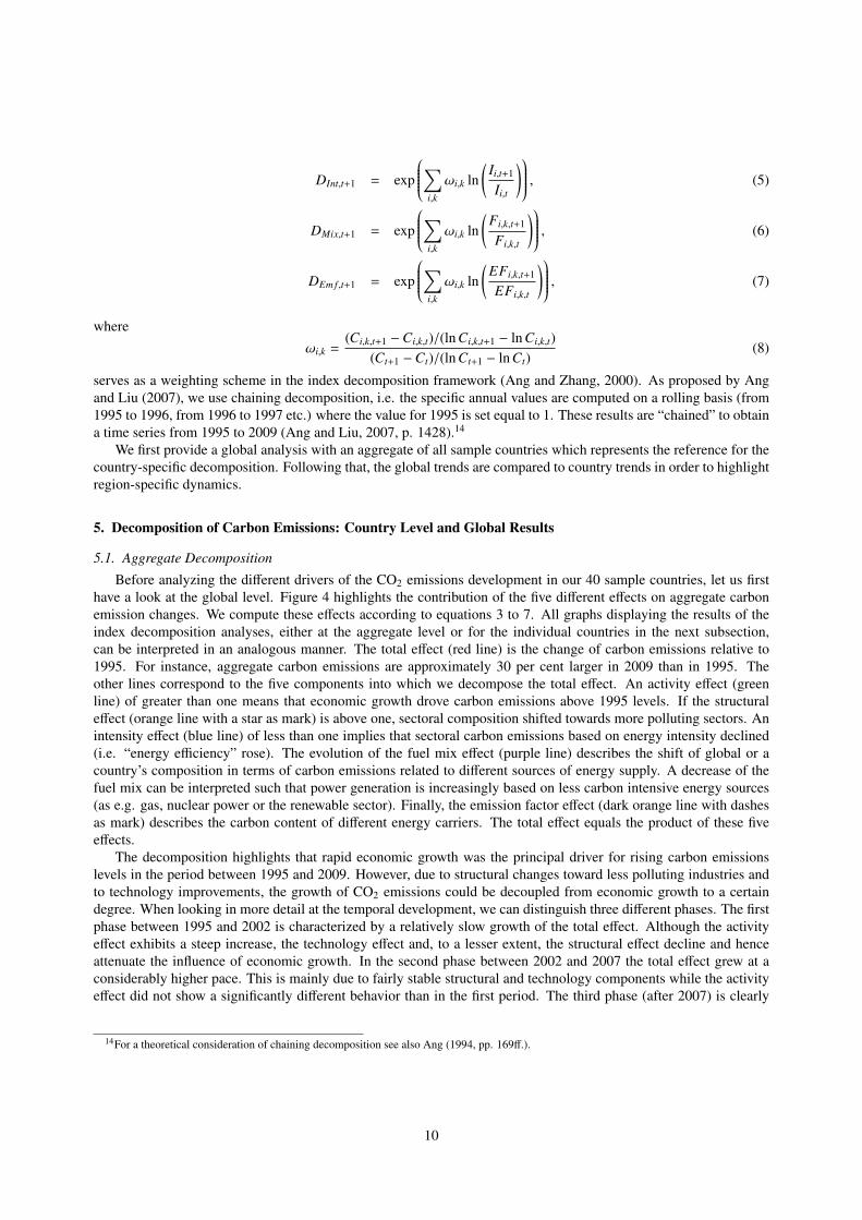
Before analyzing the different drivers of the CO2 emissions development in our 40 sample countries, let us firsthave a look at the global level. Figure 4 highlights the contribution of the five different effects on aggregate carbonemission changes. We compute these effects according to equations 3 to 7. All graphs displaying the results of theindex decomposition analyses, either at the aggregate level or for the individual countries in the next subsection,can be interpreted in an analogous manner. The total effect (red line) is the change of carbon emissions relative to1995. For instance, aggregate carbon emissions are approximately 30 per cent larger in 2009 than in 1995. Theother lines correspond to the five components into which we decompose the total effect. An activity effect (greenline) of greater than one means that economic growth drove carbon emissions above 1995 levels. If the structuraleffect (orange line with a star as mark) is above one, sectoral composition shifted towards more polluting sectors. Anintensity effect (blue line) of less than one implies that sectoral carbon emissions based on energy intensity declined(i.e. “energy efficiency” rose). The evolution of the fuel mix effect (purple line) describes the shift of global or acountry’s composition in terms of carbon emissions related to different sources of energy supply. A decrease of thefuel mix can be interpreted such that power generation is increasingly based on less carbon intensive energy sources(as e.g. gas, nuclear power or the renewable sector). Finally, the emission factor effect (dark orange line with dashesas mark) describes the carbon content of different energy carriers. The total effect equals the product of these fiveeffects.

The decomposition highlights that rapid economic growth was the principal driver for rising carbon emissionslevels in the period between 1995 and 2009. However, due to structural changes toward less polluting industries andto technology improvements, the growth of CO2 emissions could be decoupled from economic growth to a certaindegree. When looking in more detail at the temporal development, we can distinguish three different phases. The firstphase between 1995 and 2002 is characterized by a relatively slow growth of the total effect. Although the activityeffect exhibits a steep increase, the technology effect and, to a lesser extent, the structural effect decline and henceattenuate the influence of economic growth. In the second phase between 2002 and 2007 the total effect grew at aconsiderably higher pace. This is mainly due to fairly stable structural and technology components while the activityeffect did not show a significantly different behavior than in the first period. The third phase (after 2007) is clearly

14For a theoretical consideration of chaining decomposition see also Ang (1994, pp. 169ff.).

10

1995

1996

1997

1998

1999

2000

2001

2002

2003

2004

2005

2006

2007

2008

2009

0.9

1

1.1

1.2

1.3

1.4

1.5

1.6

Index

Decom

position(L

ogMeanDivisia

Index) Total Activity

Structural Intensity

Fuel Mix Emission Factor

Figure 4: LMDI decomposition of global carbon emissions

marked by a stagnation of total CO2 emissions which is, according to our calculations, a direct effect of the economiccrisis of 2008 and 2009. However, also the technology effect and the fuel mix contributed to this trend in parts.

Summarizing, the development of aggregate carbon emissions is driven by the activity, the technology and thestructural effects whereas the fuel mix and the emission factor effects played a negligible role. The most rapid declinesin the technology effect occurred between 1995 and 2001 and again between 2003 and 2008. However, in the latterphase the technology and the structural effects have opposing trends so that the steady decline in energy intensity couldnot dampen the steep increase of carbon emissions. Nevertheless, these global trends differ, in parts substantially, fromspecific country results, as we will see during the following subsection.

5.2. Country Level Decomposition

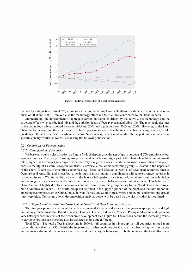
5.2.1. Classification of countriesWe base our country classification on Figure 5 which depicts growth rates of gross output and CO2 emissions of our

sample countries. The best performing group is located in the bottom right part of the chart where high output growthrates (higher than average) are coupled with relatively low growth rates of carbon emissions (lower than average). Itconsists mainly of Eastern European countries. Conversely, the worst performing group is located in the upper leftof the chart. It consists of emerging economies, e.g. Brazil and Mexico, as well as of developed countries, such asDenmark and Australia, and shows low growth rates of gross output in combination with above-average increases incarbon emissions. Within the third cluster in the bottom left, performance is mixed, i.e. these countries exhibit lowemissions growth rates (or even declines), but this is partly due to below-average output growth. This behavior ischaracteristic of highly developed economies and all countries in this group belong to the “triad” (Western Europe,North America and Japan). The fourth group can be found in the upper right part of the graph and includes importantemerging economies, such as China, India, Taiwan, Turkey and South Korea, where both output and emissions growthrates were high. Our country-level decomposition analysis below will be based on the classification just outlined.

5.2.2. IDA for Countries with Low Gross Output Growth and High Emissions GrowthThe first group consists of countries with a, compared to the world average, low gross output growth and high

emissions growth. Australia, Brazil, Canada, Denmark, Greece, Indonesia, Mexico, Portugal, Slovenia and Spain arevery heterogeneous in terms of their economic development (see Figure 6). The reasons behind the increasing trendsin carbon emissions can therefore also be expected to be quite different.

Total Effect: The total effect is above one in 2009 for all countries in this group, i.e. all countries emitted morecarbon dioxide than in 1995. While the increase was rather moderate for Canada, the observed growth in carbonemissions is substantial in countries like Brazil and particulary in Indonesia. In both countries, the total effect even

11

−1 0 1 2 3 4 5 6 7 8 9 10 11 12 13

−4

−3

−2

−1

0

1

2

3

4

5

6

7

BGRCZEEST

HUNLTU

LUX

LVA

POL

ROU

RUS

SVK

CHN

CYP

IND

IRLKOR

TURTWN

AUTBEL

DEU

FIN

FRAGBR

ITAJPN

MLT

NLD

SWEUSA

AUSBRA

CAN

DNK

ESP

GRC

IDN

MEX

PRT

SVN

Avg. ann. growth rate of gross output in % (unweighted-Ø is dotted)

Avg.

ann.

grow

thra

teof

CO

2em

issi

ons

in%

(unw

eigh

ted-Ø

isdot

ted)

Best Countries

Medium I (+ GO-Growth - CO2-Growth)

Medium II ( - GO-Growth + CO2-Growth)Worst Countries

Figure 5: Correlation between growth rates of gross output and CO2 emissions

outperforms economic growth (the activity effect). However, the drivers behind this development are different. WhileIndonesia could improve its technology and held its fuel mix almost constant, substantial structural change occurredtowards more carbon intensive sectors. In Brazil, the fuel mix trended upwards until 2001 and decreased afterwardstowards levels below 1995. Structural change played only a minor role in Brazil. A crucial cause of Brazil’s devel-opment of total carbon emissions was the use of less energy efficient technologies. In combination with substantialeconomic growth this has resulted in increasing carbon dioxide emissions in Brazil. Canada’s development of carbonemissions is a result of a slight decrease of the fuel mix effect, by significant structural change towards less carbonintensive sectors and especially by improvements of the technology effect. In combination, these three effects damp-ened the activity effect. The development of Australia’s emissions is due to economic growth which could not havebeen offset by the use of less fossil fuels or technology improvements. Together with Brazil, it is the only country witha technology effect above 1995 levels. This confirms early findings on carbon emissions in Australia by Hamiltonand Turton (2002). Denmark and two Southern European countries, Greece and Portugal, are characterized by a shifttowards more carbon intensive sectors. Their overall improvement is due to a decreasing technology effect and a shiftof the fuel mix towards less carbon emitting energy sources. While the improvement of the technology effect is almoststeady for Greece, we observe much more volatility for Denmark and Portugal. The patterns of Mexico and Spain arevery similar and the increase of the activity effect is partially compensated by a combination of decreasing technologyand fuel mix effects as well as structural change. The only Eastern European country in this group is Slovenia. Incontrast to other Eastern European countries, the Slovenian technology effect could not improve significantly. Fur-thermore, the fuel mix changed towards more carbon dioxide emitting energy carriers. The overall development ismainly due to a positive development of the structural effect.

5.2.3. IDA for Countries with Low Gross Output Growth and Low Emissions GrowthCountries with low gross output growth and low carbon emissions growth are shown in Figure 7. This group

consists exclusively of mature Western economies in Europe and North America and Japan. Not surprisingly, totalcarbon emissions have either remained rather stable or even have decreased by 2009 compared to 1995. However,the temporal development within the sample period differs to quite a high extent. France, Germany, the Netherlands,Sweden and the UK exhibit a similar path, i.e. a constant slight decline, while e.g. Italy, Japan Finland and theUS are characterized by rising emissions levels throughout most of the period but a decline towards the last yearsof our time horizon. Regarding the activity effect, the trend is very similar in all respective countries – a growing

12

1995

1996

1997

1998

1999

2000

2001

2002

2003

2004

2005

2006

2007

2008

2009

0.8

1

1.2

1.4

1.6

Index

Decomposition(L

ogMeanDivisia


Structural IntensityFuel Mix Emission Factor

(a) Australia

1995

1996

1997

1998

1999

2000

2001

2002

2003

2004

2005

2006

2007

2008

2009

0.9

1

1.1

1.2

1.3

1.4

1.5

1.6

Index

Decomposition(L

ogMeanDivisia



(b) Brazil

1995

1996

1997

1998

1999

2000

2001

2002

2003

2004

2005

2006

2007

2008

2009

0.8

1

1.2

1.4

1.6

Index

Decom

position(L

ogMeanDivisia



(c) Canada

1995

1996

1997

1998

1999

2000

2001

2002

2003

2004

2005

2006

2007

2008

2009

0.8

0.9

1

1.1

1.2

1.3

1.4

1.5

1.6

Index

Decom

position(L

ogMeanDivisia



(d) Denmark

1995

1996

1997

1998

1999

2000

2001

2002

2003

2004

2005

2006

2007

2008

2009

0.8

1

1.2

1.4

Index

Decom

position(L

ogMeanDivisia



(e) Greece

1995

1996

1997

1998

1999

2000

2001

2002

2003

2004

2005

2006

2007

2008

2009

0.8

1

1.2

1.4

1.6

1.8

2

Index

Decom

position(L

ogMeanDivisia



(f) Indonesia

1995

1996

1997

1998

1999

2000

2001

2002

2003

2004

2005

2006

2007

2008

2009

1

1.2

1.4

1.6

1.8

Index

Decom

position(L

ogMeanDivisia



(g) Mexico

1995

1996

1997

1998

1999

2000

2001

2002

2003

2004

2005

2006

2007

2008

2009

0.8

0.9

1

1.1

1.2

1.3

1.4

Index

Decom

position(L

ogMeanDivisia



(h) Portugal

1995

1996

1997

1998

1999

2000

2001

2002

2003

2004

2005

2006

2007

2008

2009

0.8

1

1.2

1.4

1.6

1.8

2

Index

Decom

position(L

ogMeanDivisia



(i) Slovenia

1995

1996

1997

1998

1999

2000

2001

2002

2003

2004

2005

2006

2007

2008

2009

0.9

1

1.1

1.2

1.3

1.4

1.5

1.6

Index

Decomposition(L

ogMeanDivisia



(j) Spain

Figure 6: IDA for countries with low gross output growth and high emissions growth

13

1995

1996

1997

1998

1999

2000

2001

2002

2003

2004

2005

2006

2007

2008

2009

0.8

1

1.2

1.4

1.6

Index

Decomposition(L

ogMeanDivisia



(a) Austria

1995

1996

1997

1998

1999

2000

2001

2002

2003

2004

2005

2006

2007

2008

2009

0.8

0.9

1

1.1

1.2

1.3

1.4

Index

Decom

position

(LogMeanDivisia



(b) Belgium

1995

1996

1997

1998

1999

2000

2001

2002

2003

2004

2005

2006

2007

2008

2009

0.8

1

1.2

1.4

1.6

1.8

Index

Decom

position

(LogMeanDivisia



(c) Finland

1995

1996

1997

1998

1999

2000

2001

2002

2003

2004

2005

2006

2007

2008

2009

0.6

0.8

1

1.2

1.4

Index

Decom

position(L

ogMeanDivisia



(d) France

1995

1996

1997

1998

1999

2000

2001

2002

2003

2004

2005

2006

2007

2008

2009

0.7

0.8

0.9

1

1.1

1.2

1.3

Index

Decom

position(L

ogMeanDivisia



(e) Germany

1995

1996

1997

1998

1999

2000

2001

2002

2003

2004

2005

2006

2007

2008

2009

0.9

1

1.1

1.2

1.3

Index

Decom

position(L

ogMeanDivisia



(f) Italy

1995

1996

1997

1998

1999

2000

2001

2002

2003

2004

2005

2006

2007

2008

2009

0.9

0.95

1

1.05

1.1

1.15

Index

Decom

position(L

ogMeanDivisia



(g) Japan

1995

1996

1997

1998

1999

2000

2001

2002

2003

2004

2005

2006

2007

2008

2009

0

0.5

1

1.5

2

2.5

Index

Decom

position(L

ogMeanDivisia



(h) Malta

1995

1996

1997

1998

1999

2000

2001

2002

2003

2004

2005

2006

2007

2008

2009

0.6

0.8

1

1.2

1.4

Index

Decom

position(L

ogMeanDivisia



(i) Netherlands

1995

1996

1997

1998

1999

2000

2001

2002

2003

2004

2005

2006

2007

2008

2009

0.7

0.8

0.9

1

1.1

1.2

1.3

1.4

1.5

Index

Decomposition(L

ogMeanDivisia



(j) Sweden

1995

1996

1997

1998

1999

2000

2001

2002

2003

2004

2005

2006

2007

2008

2009

0.8

0.9

1

1.1

1.2

1.3

1.4

1.5

Index

Decomposition(L

ogMeanDivisia



(k) United Kingdom

1995

1996

1997

1998

1999

2000

2001

2002

2003

2004

2005

2006

2007

2008

2009

0.8

0.9

1

1.1

1.2

1.3

1.4

1.5

Index

Decomposition(L

ogMeanDivisia



(l) United States

Figure 7: IDA for countries with low gross output growth and low emissions growth

14

economy until 2007/2008 and a sharp decrease thereafter. Nevertheless, Italian and particularly Japanese growth ratesare significantly smaller than those of the other countries. The structural effect is decreasing in most countries, i.e.“cleaner” sectors gained weight within the respective economies, with three exceptions – Austria, Germany and Malta– where a shift towards sectors with higher carbon emissions occurred. This is also reflected in the development ofthe technology effect in these three countries. It rapidly declines and hence compensates the increase of the structuraleffect. Especially Germany exhibits one of the greatest declines of the technology effect. In general, the pattern oftechnology improvements differs quite tremendously between the sample countries. Besides Germany, the most rapiddecreases can be observed in Austria, France, Malta, the Netherlands, Sweden and the UK. On the other hand, Italy,Japan and the United States saw a rather stable development when comparing the years 1995 and 2009. While Italyand the US experienced relatively large technology improvements in the first half of the sample period which was moreor less revoked in the second half, Japan effectively exhibited almost no change in this component. When comparingthe technology effect with the total effect, one can clearly observe similarities between them in most countries of thisgroup, inducing a strong influence of technology improvements on the development of carbon emissions. Finally,more than in any other group, the fuel mix had a considerable influence on the total effect. Except for France, Swedenand the US – with little change or only a slight decline – and Japan with a moderate increase, all countries saw adecline by almost 10% or more during the sample period, implying a shift towards cleaner fuel inputs. The path ofthe fuel mix effect is also similar to that of the total effect in many countries of this group.

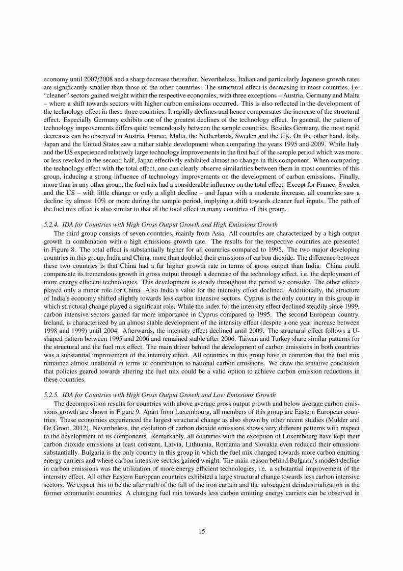
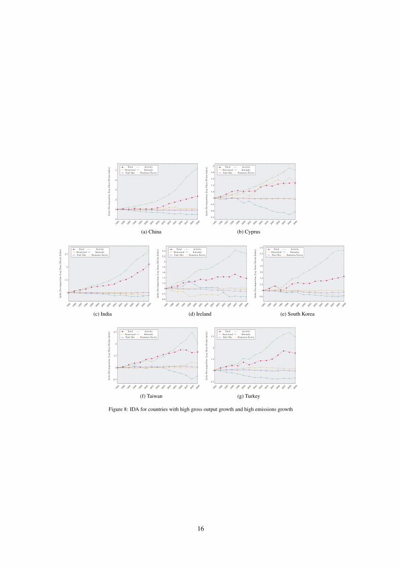
5.2.4. IDA for Countries with High Gross Output Growth and High Emissions GrowthThe third group consists of seven countries, mainly from Asia. All countries are characterized by a high output

growth in combination with a high emissions growth rate. The results for the respective countries are presentedin Figure 8. The total effect is substantially higher for all countries compared to 1995. The two major developingcountries in this group, India and China, more than doubled their emissions of carbon dioxide. The difference betweenthese two countries is that China had a far higher growth rate in terms of gross output than India. China couldcompensate its tremendous growth in gross output through a decrease of the technology effect, i.e. the deployment ofmore energy efficient technologies. This development is steady throughout the period we consider. The other effectsplayed only a minor role for China. Also India’s value for the intensity effect declined. Additionally, the structureof India’s economy shifted slightly towards less carbon intensive sectors. Cyprus is the only country in this group inwhich structural change played a significant role. While the index for the intensity effect declined steadily since 1999,carbon intensive sectors gained far more importance in Cyprus compared to 1995. The second European country,Ireland, is characterized by an almost stable development of the intensity effect (despite a one year increase between1998 and 1999) until 2004. Afterwards, the intensity effect declined until 2009. The structural effect follows a U-shaped pattern between 1995 and 2006 and remained stable after 2006. Taiwan and Turkey share similar patterns forthe structural and the fuel mix effect. The main driver behind the development of carbon emissions in both countrieswas a substantial improvement of the intensity effect. All countries in this group have in common that the fuel mixremained almost unaltered in terms of contribution to national carbon emissions. We draw the tentative conclusionthat policies geared towards altering the fuel mix could be a valid option to achieve carbon emission reductions inthese countries.

5.2.5. IDA for Countries with High Gross Output Growth and Low Emissions GrowthThe decomposition results for countries with above average gross output growth and below average carbon emis-

sions growth are shown in Figure 9. Apart from Luxembourg, all members of this group are Eastern European coun-tries. These economies experienced the largest structural change as also shown by other recent studies (Mulder andDe Groot, 2012). Nevertheless, the evolution of carbon dioxide emissions shows very different patterns with respectto the development of its components. Remarkably, all countries with the exception of Luxembourg have kept theircarbon dioxide emissions at least constant, Latvia, Lithuania, Romania and Slovakia even reduced their emissionssubstantially. Bulgaria is the only country in this group in which the fuel mix changed towards more carbon emittingenergy carriers and where carbon intensive sectors gained weight. The main reason behind Bulgaria’s modest declinein carbon emissions was the utilization of more energy efficient technologies, i.e. a substantial improvement of theintensity effect. All other Eastern European countries exhibited a large structural change towards less carbon intensivesectors. We expect this to be the aftermath of the fall of the iron curtain and the subsequent deindustrialization in theformer communist countries. A changing fuel mix towards less carbon emitting energy carriers can be observed in

15

1995

1996

1997

1998

1999

2000

2001

2002

2003

2004

2005

2006

2007

2008

2009

0

1

2

3

4

5

Index

Decom

position(L

ogMeanDivisia



(a) China

1995

1996

1997

1998

1999

2000

2001

2002

2003

2004

2005

2006

2007

2008

2009

0.4

0.6

0.8

1

1.2

1.4

1.6

1.8

2

Index

Decom

position(L

ogMeanDivisia



(b) Cyprus

1995

1996

1997

1998

1999

2000

2001

2002

2003

2004

2005

2006

2007

2008

2009

1

1.5

2

2.5

Index

Decom

position(L

ogMeanDivisia



(c) India

1995

1996

1997

1998

1999

2000

2001

2002

2003

2004

2005

2006

2007

2008

2009

0.6

0.8

1

1.2

1.4

1.6

1.8

2

2.2

2.4

Index

Decom

position(L

ogMeanDivisia



(d) Ireland

1995

1996

1997

1998

1999

2000

2001

2002

2003

2004

2005

2006

2007

2008

2009

0.8

1

1.2

1.4

1.6

1.8

2

2.2

2.4

Index

Decom

position(L

ogMeanDivisia



(e) South Korea

1995

1996

1997

1998

1999

2000

2001

2002

2003

2004

2005

2006

2007

2008

2009

0.5

1

1.5

2

2.5

Index

Decomposition(L

ogMeanDivisia



(f) Taiwan

1995

1996

1997

1998

1999

2000

2001

2002

2003

2004

2005

2006

2007

2008

2009

0.5

1

1.5

2

2.5

Index

Decomposition(L

ogMeanDivisia



(g) Turkey

Figure 8: IDA for countries with high gross output growth and high emissions growth

16

1995

1996

1997

1998

1999

2000

2001

2002

2003

2004

2005

2006

2007

2008

2009

0.4

0.6

0.8

1

1.2

1.4

1.6

1.8

2

Index

Decomposition(L

ogMeanDivisia



(a) Bulgaria

1995

1996

1997

1998

1999

2000

2001

2002

2003

2004

2005

2006

2007

2008

2009

0.6

0.8

1

1.2

1.4

1.6

1.8

2

Index

Decom

position

(LogMeanDivisia



(b) Czech Republic

1995

1996

1997

1998

1999

2000

2001

2002

2003

2004

2005

2006

2007

2008

2009

0.5

1

1.5

2

2.5

Index

Decom

position

(LogMeanDivisia



(c) Estonia

1995

1996

1997

1998

1999

2000

2001

2002

2003

2004

2005

2006

2007

2008

2009

0.4

0.6

0.8

1

1.2

1.4

1.6

1.8

2

2.2

Index

Decom

position(L

ogMeanDivisia



(d) Hungary

1995

1996

1997

1998

1999

2000

2001

2002

2003

2004

2005

2006

2007

2008

2009

0.6

0.8

1

1.2

1.4

1.6

1.8

2

2.2

Index

Decom

position(L

ogMeanDivisia



(e) Latvia

1995

1996

1997

1998

1999

2000

2001

2002

2003

2004

2005

2006

2007

2008

2009

0.6

0.8

1

1.2

1.4

1.6

1.8

2

Index

Decom

position(L

ogMeanDivisia



(f) Lithuania

1995

1996

1997

1998

1999

2000

2001

2002

2003

2004

2005

2006

2007

2008

2009

0.5

1

1.5

2

2.5

3

3.5

4

4.5

Index

Decom

position(L

ogMeanDivisia



(g) Luxembourg1995

1996

1997

1998

1999

2000

2001

2002

2003

2004

2005

2006

2007

2008

2009

0.6

0.8

1

1.2

1.4

1.6

1.8

2

2.2

2.4

Index

Decom

position(L

ogMeanDivisia



(h) Poland

1995

1996

1997

1998

1999

2000

2001

2002

2003

2004

2005

2006

2007

2008

2009

0.6

0.8

1

1.2

1.4

1.6

1.8

Index

Decom

position(L

ogMeanDivisia



(i) Romania

1995

1996

1997

1998

1999

2000

2001

2002

2003

2004

2005

2006

2007

2008

2009

0.6

0.8

1

1.2

1.4

1.6

1.8

2

Index

Decomposition(L

ogMeanDivisia



(j) Russia

1995

1996

1997

1998

1999

2000

2001

2002

2003

2004

2005

2006

2007

2008

2009

0.5

1

1.5

2

2.5

Index

Decom

position

(LogMeanDivisia



(k) Slovakia

Figure 9: IDA for countries with high gross output growth and low emissions growth

17

the Czech Republic, Hungary, Latvia, Lithuania, Romania and Slovakia. In Bulgaria, Latvia and Poland the carbonemissions development is to a very high extent determined by technology improvements. On the contrary, in Estoniaand Hungary carbon emissions development can almost entirely be assigned to structural changes of the economy.The former country even saw technological deterioration over the whole sample period while this trend was reversedin Hungary after 2002/2003.

6. Conclusion

This paper analyzes trends in carbon emissions for 40 major economies between 1995 and 2009. It contributes tothe literature in index decomposition analysis in several ways. First, so far most of the index decomposition literaturehas mainly analyzed energy intensity. This perspective is extended in our study to examine carbon emissions for a widevariety of countries. Second, it employs a novel socio-economic database consistently accompanied by environmentalsatellite accounts to construct measures of carbon emissions for 34 sectors. Based on this harmonized dataset, acomprehensive compendium of carbon emissions time series has been computed. Third, we show that – with respectto the development of CO2 emissions – heterogeneity in each country across sectors is higher than heterogeneityin sectors across countries. This finding might lead to the conclusion that structural conditions in sectors prevailover regional circumstances, such as regulatory measures. Fourth, the paper decomposes carbon emissions into fivedifferent factors, the activity effect, the structural effect, the fuel mix effect, the emission factor and the technologyeffect in order to examine what share of temporal variation is due to actual changes in the technology within theeconomy’s sectors or in the fuel mix and is hence replicable, and what share is based merely on structural changes ofthe economy.

We classify our sample countries into four groups according to the level of their gross output and CO2 emissionsgrowth rates. The best performing group – with high output and low emissions growth or even declines – consistsmainly of Eastern European countries. They reduced their carbon intensity levels by up to 60% over the sampleperiod. On the other hand, the worst performing group – with low gross output and high emissions growth – achievedmean carbon intensity reductions of approximately 10 to 15% between 1995 and 2009. However, the drivers of thisdevelopment, in particular the technological and the structural component, are very heterogeneous and we cannotgeneralize our results for the different groups. Among the world’s top ten emitters as of 2009, in only three countries– Canada, China and Germany – the main driver of carbon emission development was technology improvement.Conversely, in Japan and the United States structural change of the economy was responsible for the developmentof carbon emissions. In the other countries, i.e. India, Russia, South Korea and the United Kingdom, both effectsdrove the evolution of carbon emissions. In the US and in Russia the structural component was slightly dominant,while in India, South Korea and the UK the technology component contributed to a higher degree. At the globallevel, carbon emissions development is driven by both the technology effect as well as structural change towards lesscarbon intensive sectors. Nevertheless, absolute global CO2 emission levels increased by one third over the sampleperiod. Therefore, an important challenge for policy makers is to translate carbon intensity reduction, which can stillbe accompanied by rising emissions levels, into actual declines in CO2 emissions. Given our results of the descriptiveanalysis, an interesting approach could be to start at the sectoral level. This view is also supported by others as“sectoral approaches may be a better way to attack negative competitiveness effects and leakage. They are consistentwith desires of developing countries to curtail emissions for domestic reasons and raise fewer issues of economicimperialism” (McLure, 2014, p. 556). Another field of potential which could be leveraged are changes in the fuel mixof individual countries. While the fuel mix effect contributes to a significant extent in some European countries suchas Austria, Denmark, Germany, Greece and Italy, there seems to exist large space for improvement in other countries,e.g. Australia, China, India, Japan and the United States. Finally, the impact of emission factor changes of specificfuel types is negligible, i.e. within this relatively short time horizon carbon efficiency of fuels hardly improved.

Our analysis hence suggests some interesting directions for future research. A first step would be to explore thedeterminants of a country’s heterogeneity in performance in order to isolate those factors that can promote technolog-ical change and thus bring about long lasting improvements in carbon emissions and CO2 abatement. Finally, a casestudy analysis of those countries where the impact of the technology effect was significant is clearly worthwhile.

18

Acknowledgments

The authors gratefully acknowledge funding by the European Commission in the project “World Input-OutputDatabase: Construction and Applications” (FP7/2007-2013) under grant agreement no. 225 281 and to the GermanFederal Ministry of Education and Research within the project CliPoN under the grant agreement 01LA1105B. Theusual disclaimers apply. Moreover, we are deeply grateful to Sascha Rexhauser for valuable comments. The usualdisclaimers apply.

References

Aldy, J., Krupnick, A., Newell, R., Parry, I., Pizer, W. (2010): Designing Climate Mitigation Policy, in: Journal of Economic Literature, Vol. 48,pp. 903-934.

Ang, B.W. (1994): Decomposition of industrial energy consumption, in: Energy Economics, Vol. 16, pp. 163-174.Ang, B.W., Choi, K.-H. (1997): Decomposition of aggregate energy and gas emission intensitites for industry: a refined Divisia index method, in:

The Energy Journal, Vol. 18, pp. 59-73.Ang, B.W., Zhang, F.Q., Choi, K.-H. (1998): Factorizing changes in energy and environmental indicators through decomposition, in: Energy, Vol.

23, pp. 489-495.Ang, B.W., Zhang, F.Q. (2000): A survey of index decomposition analysis in energy and environmental studies, in: Energy, Vol. 25, pp. 1149-1176.Ang, B.W., Liu, F.L. (2001): A new energy decomposition method: perfect in decomposition and consistent in aggregation, in: Energy, Vol. 26,

pp. 537-548.Ang, B.W., Liu, N. (2007): Energy decomposition analysis: IEA model versus other methods, in: Energy Policy, Vol. 35, pp. 1426-1432.Boyd, G.A., Roop, J.M. (2004): A Note on the Fisher Ideal Index Decomposition for Structural Change in Energy Intensity, in: The Energy Journal,

Vol. 25, No. 1, pp. 87-101.Canadell, J.G., Le Quere, C., Raupach, M.R., Field, C.B., Buitenhuis, E.T., Ciais, P., Conway, T.J., Gillett, N.P., Houghton, N.A., Marland,

G., (2007): Contributions to accelerating atmospheric CO2 growth from economic activity, carbon intensity, and efficiency of natural sinks, in:Proceedings of the National Academy of Sciences, Vol. 104, pp. 18866-18870.

Chance, W.A. (1966): A Note on the Origins of Index Numbers, in: The Review of Economics and Statistics, Vol. 48, No. 1, pp. 108-110.Choi, K.-H., Ang, B.W. (2012): Attribution of changes in Divisia real energy intensity index - An extension to index decomposition analysis, in:

Energy Economics, Vol. 34, pp. 171-176.Diewert, E.W. (1993): Index Numbers, in: Essays in Index Number Theory, Vol. 1, No. 1, Chapter 5, pp. 71-109.Dietzenbacher, E., Los, B., Stehrer, R., Timmer, M.P., De Vries, G.J. (2013): The construction of world input-output tables in the WIOD project,

in Economic Systems Research, Vol. 25, No. 1, pp. 71-98.Greening, L.A., Davis, W.B., Schipper, L. (1998): Decomposition of aggregate carbon intensity for the manufacturing sector: comparison of

declining trends from 10 OECD countries for the period 1971-1991, in: Energy Economics, Vol. 20, pp. 43-65.Greening, L.A. (2004): Effects of human behavior on aggregate carbon intensity of personal transportation: comparison of 10 OECD countries for

the period 1970–1993, in: Energy Economics, Vol. 26, pp. 1-30.Hamilton, C., Turton, H. (2002): Determinants of emissions growth in OECD countries, in: Energy Policy, Vol. 30, pp. 63-71.IEO (2013), International Energy Outlook 2013, U.S. Energy Information Administration, U.S. Department of Energy, Washington, DC.Kim, K., Kim, Y. (2012): International comparison of industrial CO2 emission trends and the energy efficiency paradox utilizing production-based

decomposition, in: Energy Economics, Vol. 34, pp. 1724-1741.Lange, A., Loschel, A., Vogt, C., Ziegler, A. (2006): On the Self-Interested Use of Equity in International Climate Negotiations, in: European

Economic Review, Vol. 54, pp. 359-375.Ma, C., Stern, D.I. (2008): China’s changing energy intensity trend: A decomposition analysis, in: Energy Economics, Vol. 30, No. 3, pp.

1037-1053.McLure, C.E. (2014): Selected International Aspects of Carbon Taxation, in: American Economic Review Papers & Proceedings, Vol. 104, No. 5,

pp. 552556.Mulder, P., De Groot, H.L.F. (2012). Structural change and convergence of energy intensity across OECD countries, 1970-2005, in: Energy

Economics, Vol. 34, pp. 1910-1921.OECD (2012): OECD Environmental Outlook to 2050, OECD Publishing. http://dx.doi.org/10.1787/9789264122246-enRaupach, M.R., Marland, G., Ciais, P., LeQuere, C., Canadell, J.G., Klepper, G., Field, C.B. (2007): Global and regional drivers of accelerating

CO2 emissions, in: Proceedings of the National Academy of Sciences, Vol. 104, pp. 10288-10293.Su, B., Ang, B.W. (2012): Structural decomposition analysis applied to energy and emissions: Some methodological developments, in: Energy

Economics, Vol. 34, pp. 177-188.Voigt, S., De Cian, E., Schymura, M., Verdolini, E. (2014): Energy Intensity Developments in 40 Major Economies: Structural Change or

Technology Improvement?, in: Energy Economics, Vol. 41, pp. 47-62.WIOD (2012): World Input-Output Database: Construction and Applications, FP7-funded project. http://www.wiod.org/

19

What Drives Changes in Carbon Emissions? An Index ...

Documents

Transcript of What Drives Changes in Carbon Emissions? An Index ...