
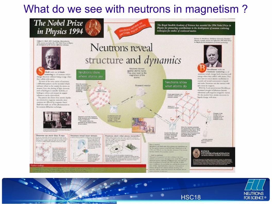
What do we see with neutrons in magnetism · What do we see with neutrons in magnetism ?...
64
JDN20—Diffraction , L. Chapon HSC18 L.C. Chapon Institut Laue-Langevin, Grenoble, France What do we see with neutrons in magnetism ?
Transcript of What do we see with neutrons in magnetism · What do we see with neutrons in magnetism ?...

JDN20—Diffraction , L. Chapon
HSC18
L.C. ChaponInstitut Laue-Langevin, Grenoble, France
What do we see with neutrons in magnetism ?

JDN20—Diffraction , L. Chapon
HSC18
The neutron
+2/3 -1/3
-1/3
● Non-charged particle
● Total angular momemtum (« nuclear spin ») I=1/2● The magnetic moment is extremely small compared to the electron.
-> The interaction potential is small, Born approximation is valid
N=eℏ
2mp
=5.0510−27 J.T−1
B=e ℏ
2me
=9.2810−24 J.T −1
mN=1.67.10−27 kg
= N with=−1.913

JDN20—Diffraction , L. Chapon
HSC18
Production : Nuclear fission
JDN20—Diffraction , L. Chapon
HSC18
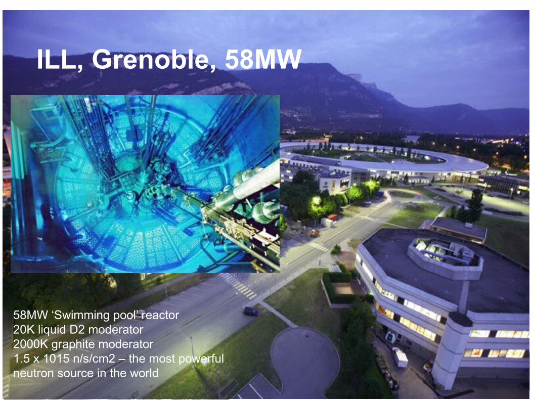
ILL, Grenoble, 58MW
58MW ‘Swimming pool’ reactor20K liquid D2 moderator2000K graphite moderator1.5 x 1015 n/s/cm2 – the most powerful neutron source in the world

JDN20—Diffraction , L. Chapon
HSC18
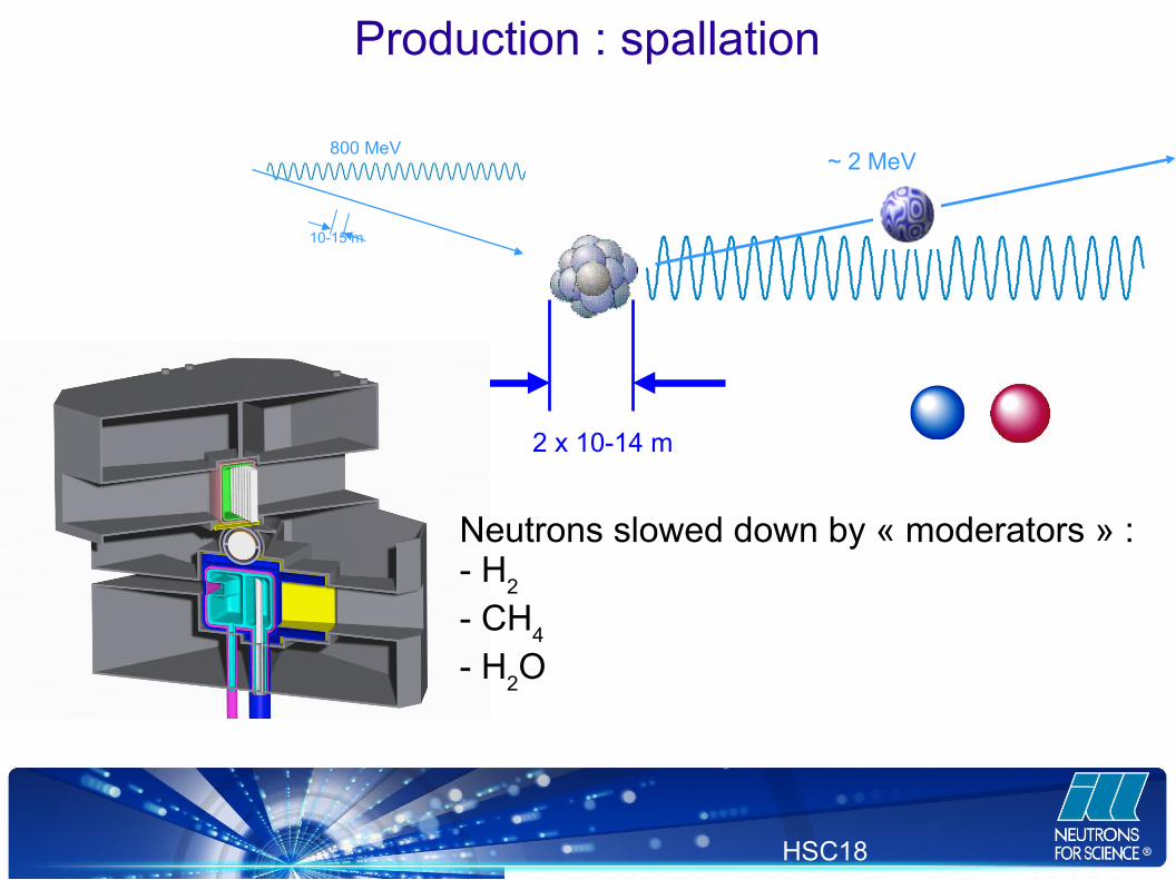
Production : spallation

HSC18
800 MeV
HSC18
2 x 10-14 m
10-15 m
800 MeV~ 2 MeV
Neutrons slowed down by « moderators » :- H
2
- CH4
- H2O
Production : spallation
JDN20—Diffraction , L. Chapon
HSC18
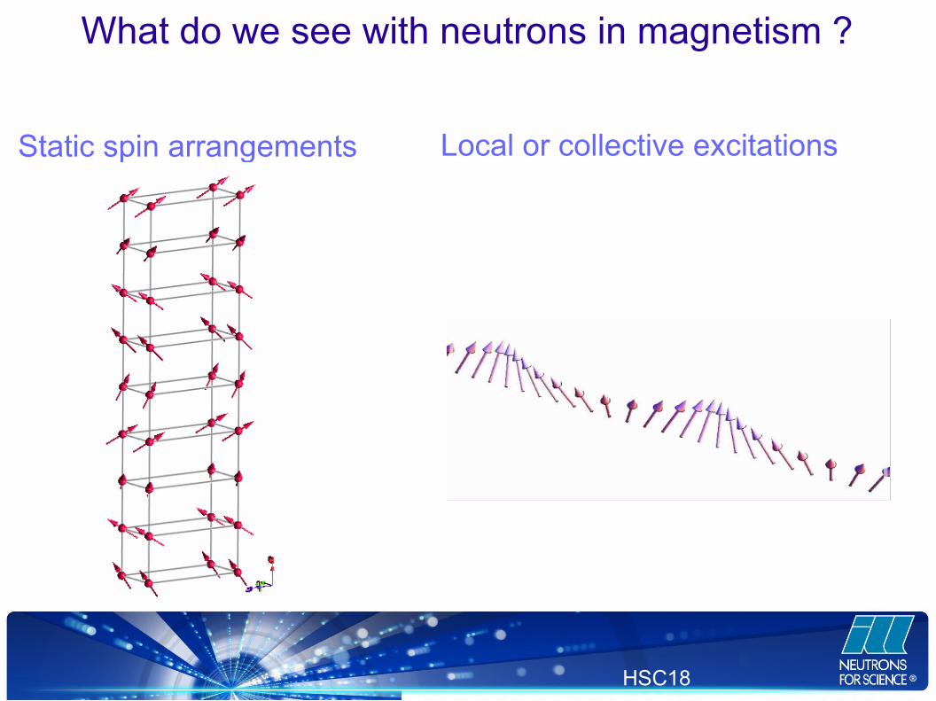
What do we see with neutrons in magnetism ?
JDN20—Diffraction , L. Chapon
HSC18
Local or collective excitationsStatic spin arrangements
What do we see with neutrons in magnetism ?

JDN20—Diffraction , L. Chapon
HSC18
Outline
● Reminder of scattering theory, neutron nuclear scattering● Magnetic scattering theory:
– Spin contribution– Orbital contribution– Density matrix formalism, non-polarized and polarized cases – Magnetic form factors
● Probing different magnetic states: – Magnetic Bragg scattering: Long-range ordered structures– Diffuse scattering, short-range correlations– Small angle scattering, skyrmions– Inelastic scattering, crystal field excitations, magnons

JDN20—Diffraction , L. Chapon
HSC18
Scattering by a potential V(r)
●has the dimension of a surface● Usually in barns=1024 cm2
●has the dimension of a surface● Usually in barns=1024 cm2
V(r)
Flux
d
dn⏞n. s−1
= Φ⏞n. cm−2. s−1
dΩ⏞n . u
σ (θ , φ)
●has the dimension of a surface● Usually in barns=1024 cm2

JDN20—Diffraction , L. Chapon
HSC18
Differential cross section, Fermi's Golden rule
d2σ
dΩdE'=∑
λ
pλ ∑λ '
(d2σ
dΩdE')λ→λ '
=k 'k
(m
2πℏ2)
2
∑λ
pλ∑λ '
|⟨k ' λ '|V|k λ ⟩|2 δ(Eλ−Eλ '+ E−E ')
V(r)Neutron E, k, sample state
Neutron E', k', sample state '

JDN20—Diffraction , L. Chapon
HSC18
Born approximation
[k2] r =
2
ℏ2
V r r
●In the integral equation of scattering, the stationary wave-function is written :
σk(θ ,φ)=m2
4π2 ℏ2 ∣∫V (r )ei Qr d3 r∣2
●In the quantum mechanical treatment of scattering by a central potential, the stationary states (r) verify:
Quantum Mechanics, Claude Cohen-Tannoudji et al., Vol 2, Chapt 8
vkscat
r =eiki.r2
ℏ2 ∫G+r −r 'V r 'vkscat
r 'd3r '
●One can expend iteratively this expression (Born expansion).If the potential is weak, one can limit the expansion to the first term, this is the firstBorn approximation. In this case the scattering cross section (amplitude) is related to the Fourier transform of the potential function.
JDN20—Diffraction , L. Chapon
HSC18
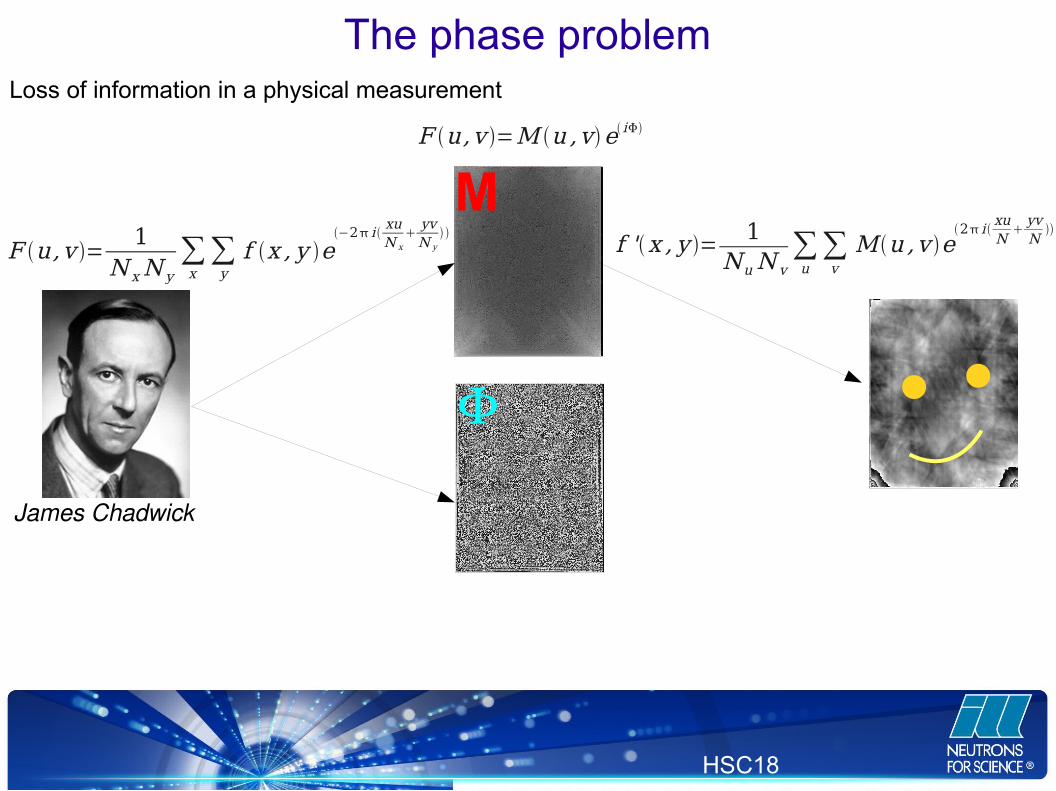
The phase problem
F u,v =1
N x N y∑
x∑
yf x , y e
−2 i xuN x
yvN y
James Chadwick
M
f 'x , y =1
Nu N v∑
u∑
v
M u ,v e2 i
xuN
yvN
F u,v =M u ,ve i
Loss of information in a physical measurement
JDN20—Diffraction , L. Chapon
HSC18
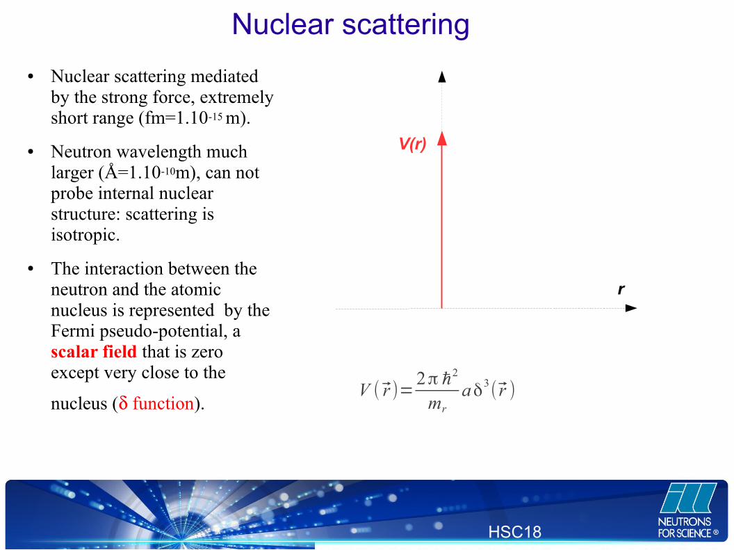
Nuclear scattering
V(r)
r
● Nuclear scattering mediated by the strong force, extremely short range (fm=1.10-15 m).
● Neutron wavelength much larger (Å=1.10-10m), can not probe internal nuclear structure: scattering is isotropic.
● The interaction between the neutron and the atomic nucleus is represented by the Fermi pseudo-potential, a scalar field that is zero except very close to the
nucleus ( function). V ( r )=2π ℏ2
mr
aδ3( r )

JDN20—Diffraction , L. Chapon
HSC18
Scattering lengths
Typically a few fm
JDN20—Diffraction , L. Chapon
HSC18
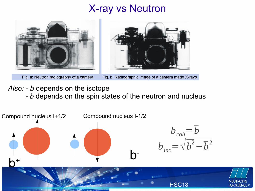
X-ray vs Neutron
Also: - b depends on the isotope - b depends on the spin states of the neutron and nucleus
Compound nucleus I+1/2 Compound nucleus I-1/2
b+ b-
bcoh=b
b inc=b2−b2

JDN20—Diffraction , L. Chapon
HSC18
Magnetic cross section
For elastic neutron magnetic scattering, one needs to evaluate (in the Born approximation), the cross section:
(d 2 σ
dΩdE ')σ ,λ→σ ' , λ '
=k 'k ( m
2 πℏ )2
|⟨k ' ,σ '|V m|k ,σ ⟩|2δ(Eλ−Eλ '+ℏω)
initial spin-state of the neutron ' final spin-state of the neutron k
incident wave-vector
k' scattered wave-vector Q momentum transfer V
m magnetic interaction potential
ki
kfQ
JDN20—Diffraction , L. Chapon
HSC18
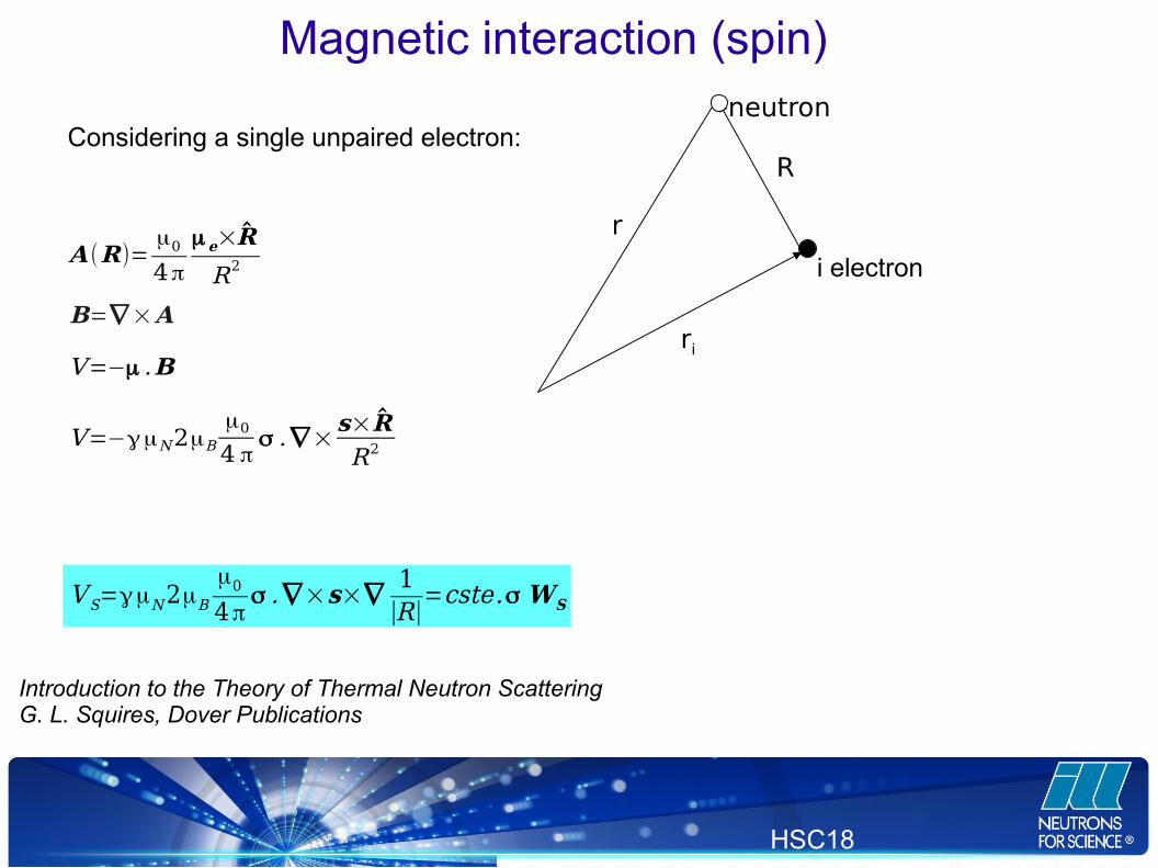
ri
r
R
neutron
Introduction to the Theory of Thermal Neutron ScatteringG. L. Squires, Dover Publications
A (R)=μ0
4π
μ e×R
R2
B=∇ ×A
V=−μ .B
V=−γμN2μB
μ0
4 πσ . ∇ ×
s×RR2
Magnetic interaction (spin)
V S=γμN2μB
μ0
4πσ . ∇×s×∇
1|R|
=cste.σ WS
Considering a single unpaired electron:
i electron

JDN20—Diffraction , L. Chapon
HSC18
Introduction to the Theory of Thermal Neutron ScatteringG. L. Squires, Dover Publications
Magnetic interaction (spin)
∇ ×s×∇1
|R|=
1
2π2 ∫1
x2 ∇ ×s×∇ eix R d x=1
2π2∫ ( x×s×x )eix R d x
⟨k '|∇ × s×∇1
|R||k ⟩= 1
2π2∫ eiQ r∫ ( x×s× x )e i x R d x d r=4 πQ×s×Q .eiQ r
i
This quantity is the projection of s perpendicular to Q:
s⊥ (Q)=Q×s×Q
⟨ k '|W s|k ⟩=4π Q×s×Q .ei .Q .r i
s
Q
s ⊥

JDN20—Diffraction , L. Chapon
HSC18
Magnetic interaction (orbital)
B(R )=μ0
4π
Idl×RR2 =
μ0 e
4 πmN
pi×R
R2 =2μ0μB
4π ℏ
pi×R
R2
V L=γμN2μB
μ0
4πℏσ . pi×∇
1|R|
=cste σ . WL
ri
r
R
neutron
i electron
Idl
WL=1ℏ
p i×R
R2
⟨ k '|W L|k ⟩=4π iℏ Q
p i×Q eiQ r i
Use the Fourier transform:
∫ R
R 2 ei κ R
=4 π i κκ

JDN20—Diffraction , L. Chapon
HSC18
Magnetic interaction strength
(d 2 σ
dΩdE ')k ,σ → k ' ,σ '
=k 'k ( m
2πℏ )2
|⟨ k ' ,σ '|V S+V L|k ,σ ⟩|2δ ...=(
m2πℏ
2 γμN μ Bμ0)2 k 'k
...
Collecting the pre-factors …..
(m
2πℏ2 γμN μ Bμ0)
2
=(γ r 0)2
r0 : free electron radius =2.8.10-15 m
Magnetic scattering length is comparable in magnitude to nuclear scattering !
Magnetic scatteringL. Chapon et al.

JDN20—Diffraction , L. Chapon
HSC18
(Spin + orbital) magnetic scattering
(d 2 σ
dΩdE ')σ ,λ→σ ' , λ '
=k 'k ( m
2 πℏ )2
|⟨k ' ,σ ' ,λ '|V m|k ,σ ,λ ⟩|2δ (E λ−Eλ '+ℏ ω)
M ⊥ =∑i
eiQ .r i (Q×si×Q+i
ℏQpi×Q)
(d 2 σ
dΩdE ')σ ,λ→σ ' , λ '
=k 'k
( γ r0 )2|⟨ λ ' ,σ '|σ .M ⊥|λ ,σ ⟩|
2δ (E λ−Eλ ' +ℏ ω)
Defining:
The spin and orbital part of M┴
are the transverse components of the Fourier transform of the spin and orbital magnetization density

JDN20—Diffraction , L. Chapon
HSC18
Density matrix formalism
ρ=∑i
p i|ψi ⟩ ⟨ ψi|
Suppose a quantum system in a mixed state, i.e. probability p1 to be in state 1, ….
probability pi to be in state i etc....
One defines a density operator
Chosen an orthonormal basis, |un>, one can define a density matrix whose elements are
ρmn=⟨um|ρ|un ⟩
⟨A ⟩=tr (ρ A)
The expectation value of an operator A is simply:
Fano, U. Description of States in Quantum Mechanics by Density Matrix and Operator Techniques Rev. Mod. Phys., American Physical Society, 1957, 29, 74-93
Calculations are enormously simplified by using the density-matrix formalism to describe mixed-states, incomplete polarization of beam, analysis....

JDN20—Diffraction , L. Chapon
HSC18
Density matrix formalism - Neutron spin states
|↑⟩=|1/2,1/2 ⟩
|↓⟩=|1/2,−1/ 2 ⟩
σ x=(0 11 0) σ y=(0 −i
i 0 ) σ z=(1 00 −1)
Pauli spin operators and matrices:
Neutron, a spin ½ particle
Spin operators:
S+|↑⟩=0
S-|↑⟩=|↓ ⟩
S+|↓⟩=|↑ ⟩
S-|↓⟩=0
Sz|↑ ⟩=1/2|↑⟩
Sz|↓ ⟩=−1/2|↓ ⟩
S+|↑⟩=0
σ x=2 S x , σ y=2 S y , σ z=2 Sz
S+=S x+i S y
S-= Sx−i S y
Density matrix representing the incident neutron beam polarization (P):
ρ=12
( I+P . σ )=12
( I+ Px . σ x+Py . σ y+Pz . σ z )
P

JDN20—Diffraction , L. Chapon
HSC18
A very easy way to averaging over all spin states:
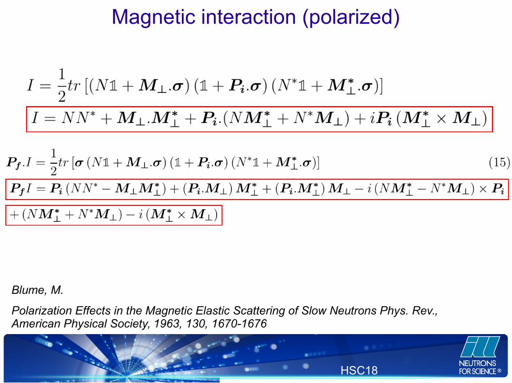
Magnetic interaction(elastic case)
d σ
dΩ=( γ r 0 )
2 tr [ (M ⊥ .σ )ρ (M ⊥ .σ )+ ]
P f .d σ
dΩ=(γ r 0)
2 tr [σ f (M ⊥ .σ )ρ (M ⊥ .σ )+ ]
Scattered intensity:
Final polarization:
Blume, M.
Polarization Effects in the Magnetic Elastic Scattering of Slow Neutrons Phys. Rev., American Physical Society, 1963, 130, 1670-1676
JDN20—Diffraction , L. Chapon
HSC18
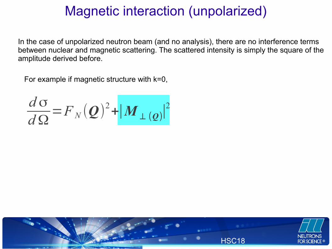
Magnetic interaction (unpolarized)
In the case of unpolarized neutron beam (and no analysis), there are no interference terms between nuclear and magnetic scattering. The scattered intensity is simply the square of the amplitude derived before.
For example if magnetic structure with k=0,
d σ
dΩ=F N (Q)
2+∣M ⊥ (Q )∣
2
JDN20—Diffraction , L. Chapon
HSC18
Magnetic interaction (polarized)
Blume, M.
Polarization Effects in the Magnetic Elastic Scattering of Slow Neutrons Phys. Rev., American Physical Society, 1963, 130, 1670-1676

JDN20—Diffraction , L. Chapon
HSC18
Magnetic “extinction”
M (Q)
Q
M ⊥
(Q)
From the projection operation emerges a very important extinction condition (if M parallel to Q, scatteringis null)
However, the only directional information about M(Q) comes from the projection operation, so great lossof information from this projection. We are only sensitive to the norm of the interaction vector.
We will see that using polarized neutrons (3D polarimetry) allows to access directlythe direction information (and phase).

JDN20—Diffraction , L. Chapon
HSC18
Magnetic “extinction” (comparison with X-ray)
Scattering amplitude (
Scattering amplitude (
−i. M (Q) . k i×k f
−2.i.sin2(θ) .M (Q) . k i
In non-resonant X-ray magnetic scattering, the cross-section depends upon projections on k
i, k
f
Consequence: signal depends on the azimuthal angle

JDN20—Diffraction , L. Chapon
HSC18
Unit-cell magnetic structure factor
Need to take into account the spatial distribution of the electron-spins and sum over allmagnetic sites in the unit-cell:
i
M (Q)=∑ jf j(Q) .m j . T j (Q)e iQ . r j
f j(Q)=1
∣m j∣∫m j(R)e iQ R d R Magnetic form factor:
Thermal parameter (Debye-Waller factor): T j (Q)
M ⊥ (Q)=Q×M (Q)×Q=M (Q)−(M (Q) . Q) .Q
Magnetic structure factor (complex vector)
Magnetic interaction vector (complex vector)
JDN20—Diffraction , L. Chapon
HSC18
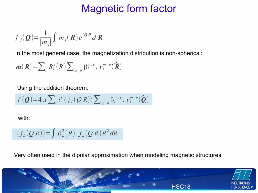
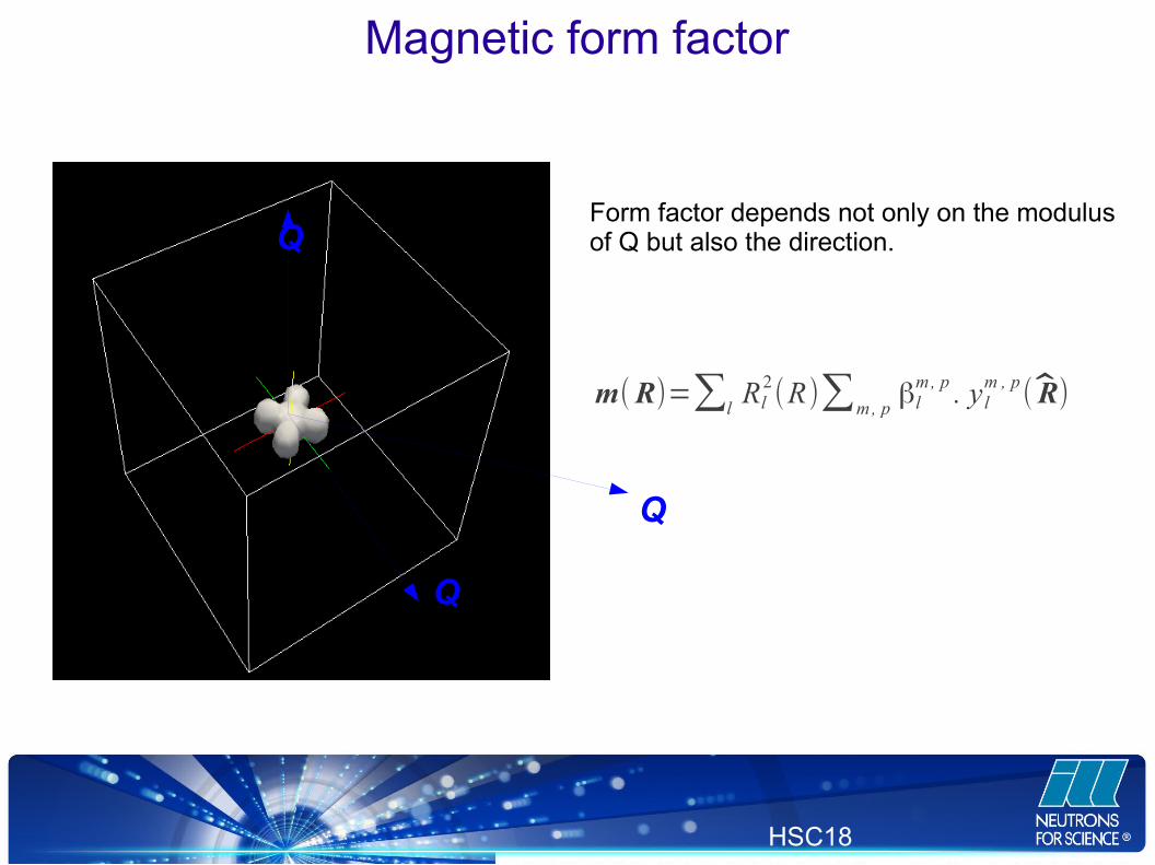
Magnetic form factor
f j(Q)=1
∣m j∣∫m j(R)e iQ R d R
m(R)=∑lRl
2(R)∑m, p
βlm , p . y l
m , p( R)
In the most general case, the magnetization distribution is non-spherical:
f (Q)=4 π∑liL ⟨ j L(Q.R)⟩∑m, p
βlm , p . y l
m , p(Q)
Using the addition theorem:
with:
⟨ jL (Q.R)⟩=∫RL2 (R) . jL (Q.R )R2dR
Very often used in the dipolar approximation when modeling magnetic structures.
JDN20—Diffraction , L. Chapon
HSC18
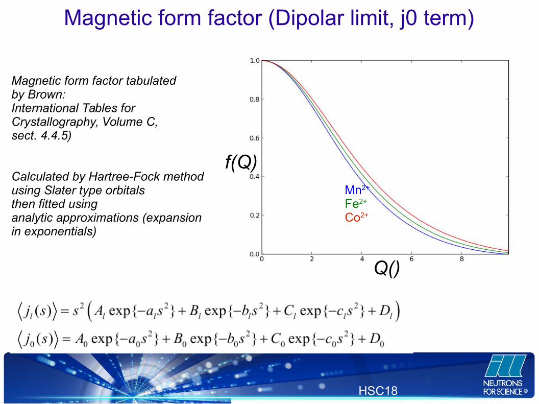
Magnetic form factor (Dipolar limit, j0 term)
f(Q)
Q(Å)
Mn2+
Fe2+
Co2+
Magnetic form factor tabulatedby Brown:International Tables for Crystallography, Volume C, sect. 4.4.5)
Calculated by Hartree-Fock methodusing Slater type orbitalsthen fitted using analytic approximations (expansion in exponentials)
Q()

JDN20—Diffraction , L. Chapon
HSC18
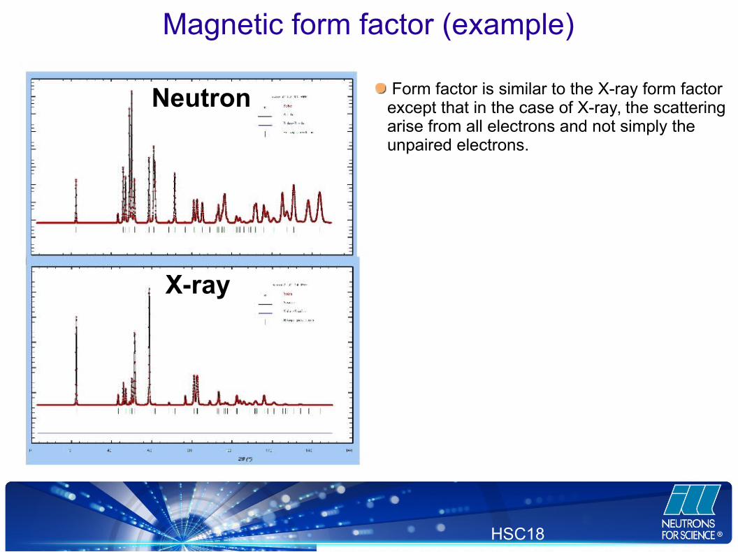
Magnetic form factor (example)
YMn2O
5
Magnetic scattering

JDN20—Diffraction , L. Chapon
HSC18
Magnetic form factor (dipolar limit, j0,j2)
In the dipole approximation:
International Tables of Crystallography, Volume C, ed. by AJC Wilson, Kluwer Ac. Pub., 1998, p. 513
)()2
1()()( 20 Qjg
QjQf
JDN20—Diffraction , L. Chapon
HSC18
Neutron
X-ray
Magnetic form factor (example)
Form factor is similar to the X-ray form factorexcept that in the case of X-ray, the scattering arise from all electrons and not simply the unpaired electrons.
JDN20—Diffraction , L. Chapon
HSC18
Magnetic form factor
Form factor depends not only on the modulusof Q but also the direction.
Q
Q
Q
m(R)=∑lRl
2(R)∑m, p
βlm , p . y l
m , p( R)

JDN20—Diffraction , L. Chapon
HSC18
Examplesof magnetic scattering
experiments
JDN20—Diffraction , L. Chapon
HSC18
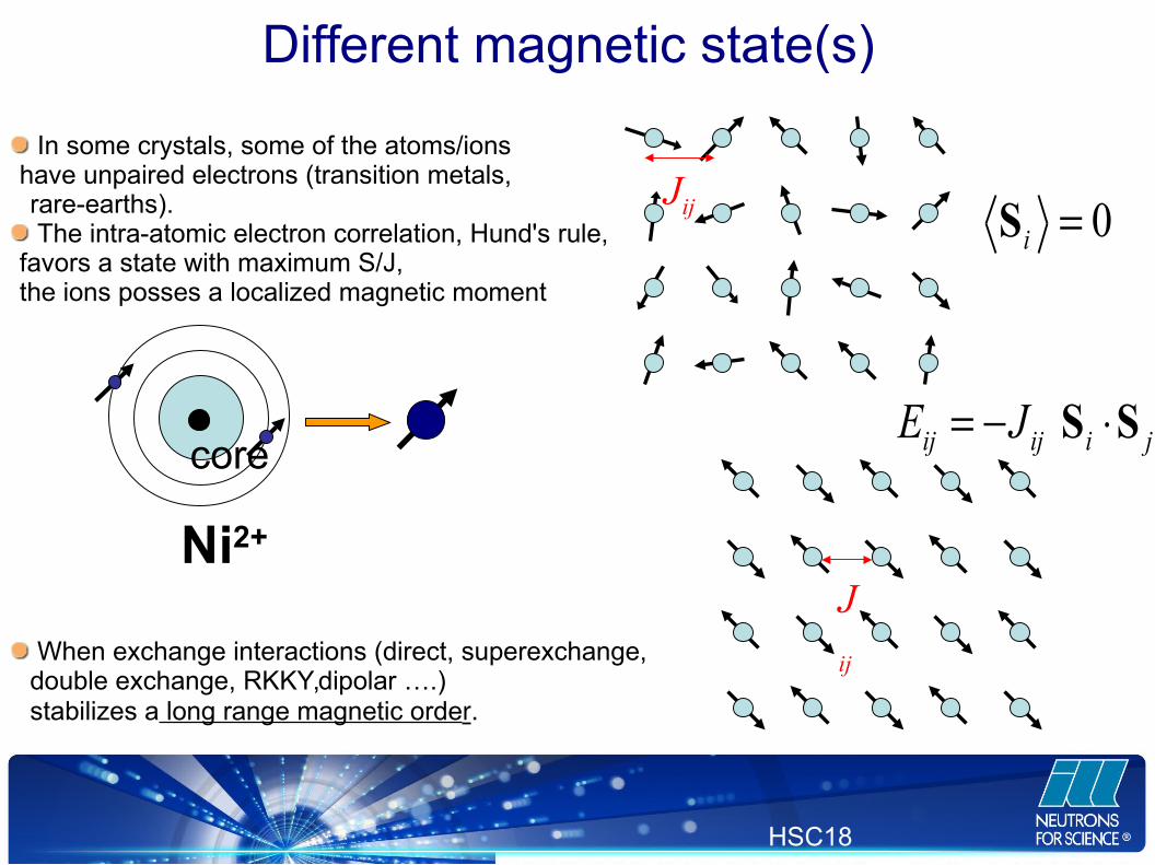
Different magnetic state(s)
Jij
S Sij ij i jE J
0Si
In some crystals, some of the atoms/ions have unpaired electrons (transition metals,rare-earths). The intra-atomic electron correlation, Hund's rule,
favors a state with maximum S/J,the ions posses a localized magnetic moment
core
Ni2+
J
ij When exchange interactions (direct, superexchange, double exchange, RKKY,dipolar ….) stabilizes a long range magnetic order.

JDN20—Diffraction , L. Chapon
HSC18
Different magnetic state(s)
● Direct exchange interaction (direct overlap of orbital wave-functions)AFM for short-distance
● Indirect exchange interaction● Super-exchange (M-O-M)● Super super-exchange (M-O-O-M)coupling through a diamagnetic anion ormore complex exchange paths
D
●RKKY interactions (coupling of localized moments through conduction electrons)
●Dipole-dipole interaction. Decrease rapidly with distance. Usually relevant for large moments at low T
JDN20—Diffraction , L. Chapon
HSC18
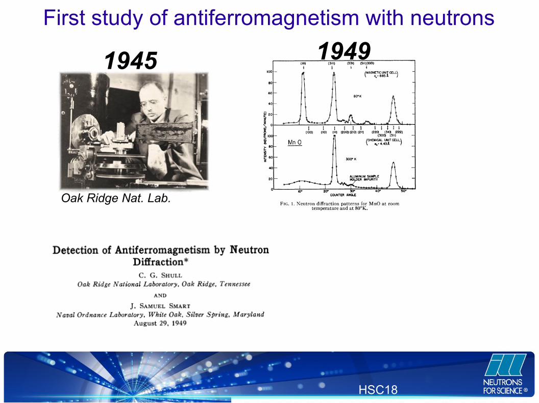
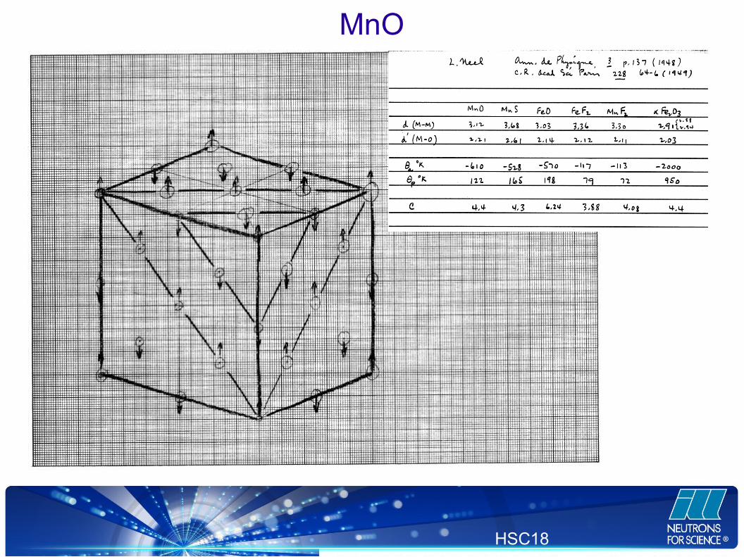
First study of antiferromagnetism with neutrons
19491945
Oak Ridge Nat. Lab.
JDN20—Diffraction , L. Chapon
HSC18
MnO
JDN20—Diffraction , L. Chapon
HSC18
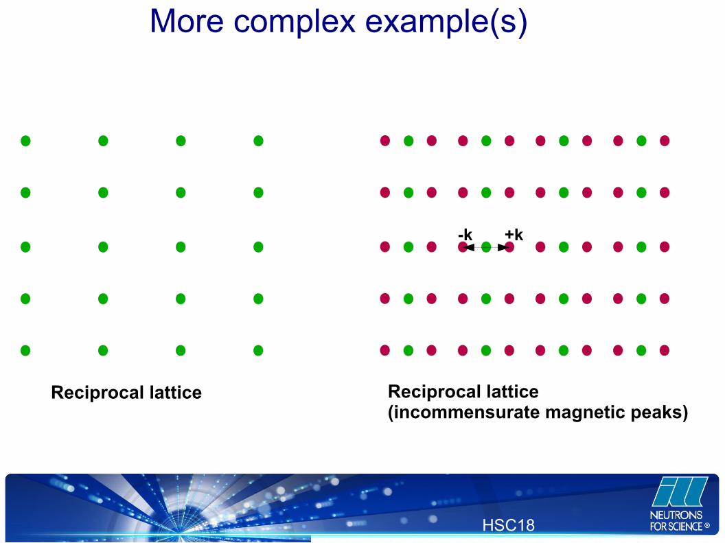
More complex example(s)
Reciprocal lattice Reciprocal lattice (incommensurate magnetic peaks)
+k-k

JDN20—Diffraction , L. Chapon
HSC18
For simplicity, in particular for wave-vector inside the BZ, one usually describe magnetic structures with Fourier components:
mlj (RL)=∑k
Skj . e−2π ik .RL
which for asingle propagation vector :mlj (RL)=Skj .e
−2π ik .RL+S−kj . e2πi k .RL
Since mlj is a real vector,
one must imposes the condition S-kj
*=Skj
Here Skj is a complex vector made of linear combinations of basis vectors that, in
the most general case, do not span necessary the same irreducible representations.
Formalism of propagation vector(s)

JDN20—Diffraction , L. Chapon
HSC18
k inside BZ- k interior of the Brillouin zone (pair k, -k)
Helix
Cycloid
Amplitude modulation

JDN20—Diffraction , L. Chapon
HSC18
Quite complex ordered states (RMn2O
5)
YMn3+
Mn4+AFM magnetic chains (ab-plane)Cycloidal component (c-direction)
k=(1/2, 0, 1/4)

JDN20—Diffraction , L. Chapon
HSC18
HoMn2O5
381 independent reflections53 refined parameters:{Rx-Ry-Iz-MagPh(Mn3+ fixed)-ext4}
m(Mn4+)=2 μB
m(Mn3+)=2.5 μB
m(Ho)=0/1 μB
YMn2O5
355 independent reflections 37 refined parameters:{Rx-Ry-Iz-MagPh(Mn3+ fixed)-ext4}
m(Mn4+)=2.4μB
m(Mn3+)=3.1 μB
BiMn2O5
204 independent reflections24 refined parameters:{Rx-Ry-Rz-ext4}
m(Mn4+)=2.1 μB
m(Mn3+)=2.8 μB
Quite complex ordered states (RMn2O
5)
JDN20—Diffraction , L. Chapon
HSC18
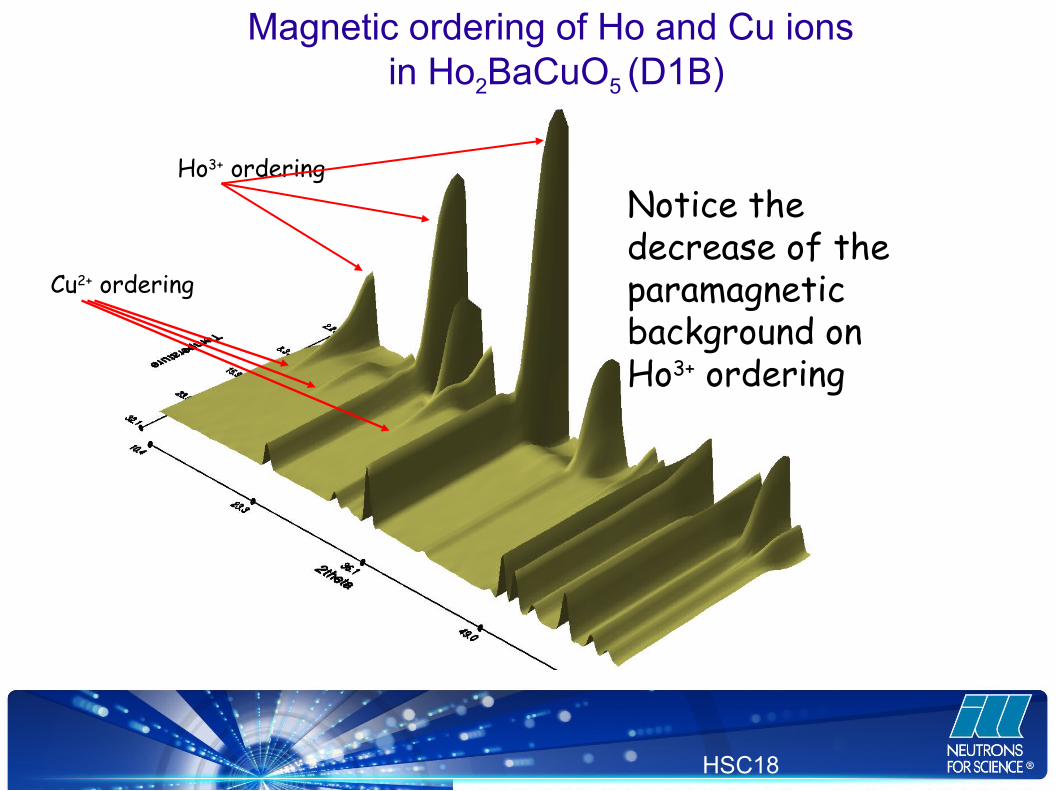
Magnetic ordering of Ho and Cu ions in Ho2BaCuO5 (D1B)
Cu2+ ordering
Ho3+ orderingNotice the decrease of the paramagnetic background on Ho3+ ordering

JDN20—Diffraction , L. Chapon
HSC18
Competing multi-q magnetic structures in HoGe3 (I & II)
P Schöbinger-Papamantellos, J Rodríguez-Carvajal, LD Tung,C Ritter and KHJ BuschowJ. Physics: Condensed Matter 20 (2008) 195201 (12pp)
195202(13pp)

JDN20—Diffraction , L. Chapon
HSC18
Conical
Multi-k structure: conical example
Multi-k structure with:
● Helical modulation
● Ferromagnetic component
JDN20—Diffraction , L. Chapon
HSC18
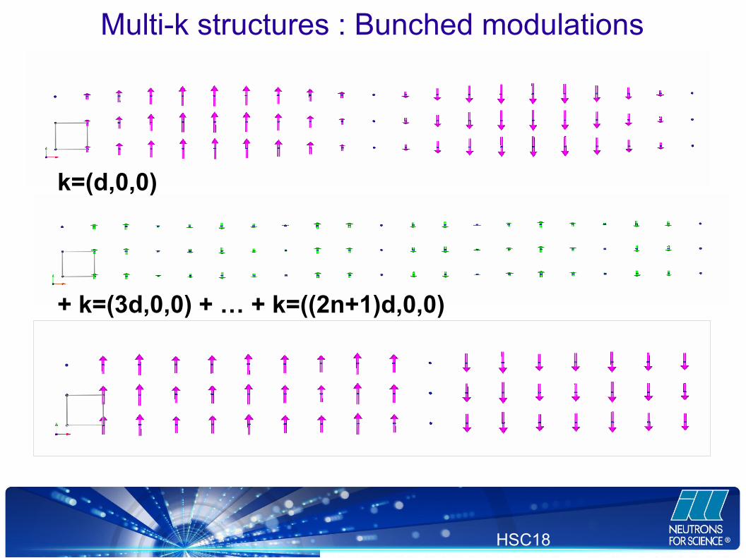
Multi-k structures : Bunched modulations
k=(d,0,0)
+ k=(3d,0,0) + … + k=((2n+1)d,0,0)

JDN20—Diffraction , L. Chapon
HSC18
TbMnO3
Kenzelmann, PRL 95, 087206 (2005)

JDN20—Diffraction , L. Chapon
HSC18
Multi-k structures
Example of a 4-k structure: the skyrmion lattice
k1
k2
k3
● k1+k
2+k
3=0, same chirality for k
1, k
2, k
3
● Ferromagnetic component

JDN20—Diffraction , L. Chapon
HSC18
Multi-k structures
“Skyrmion”-type lattice stabilized by energy terms of the type:
F=...+S 1eik 1 +ϕ1 . S 2 e
ik 2+ϕ2 . S 3 eik 3+ϕ3 . M

JDN20—Diffraction , L. Chapon
HSC18
Skyrmion in MnSi

JDN20—Diffraction , L. Chapon
HSC18
Domains
Because the symmetry of the ordered magnetic state is lower than that of the paramagnetic state (loss of certain symmetry elements)
If the order of the paramagnetic group G0 is g and the order of the ordered
group G1 is h, there will be g/h domains.
The different types of domains:
configuration domains (k-domains) : loss of translational symmetry
orientation domains (S-domains): loss of rotational symmetry
180 degrees domains (time-reversed domains): loss of time-reversal symmetry
chiral domains: loss of inversion symmetry

JDN20—Diffraction , L. Chapon
HSC18
Chiral-domains
Loss of inversion symmetry generates two domains of opposite handedness
Note however that this is not the case if the paramagnetic group is a chiral group, in which case a single handedness is stabilized (no energy degeneracy)

JDN20—Diffraction , L. Chapon
HSC18
Inversion domains (“chiral” scattering)
Spherical Polarimetry, ILL CRYOPAD
Skℑ(M ⊥ ×M ⊥
*)
JDN20—Diffraction , L. Chapon
HSC18
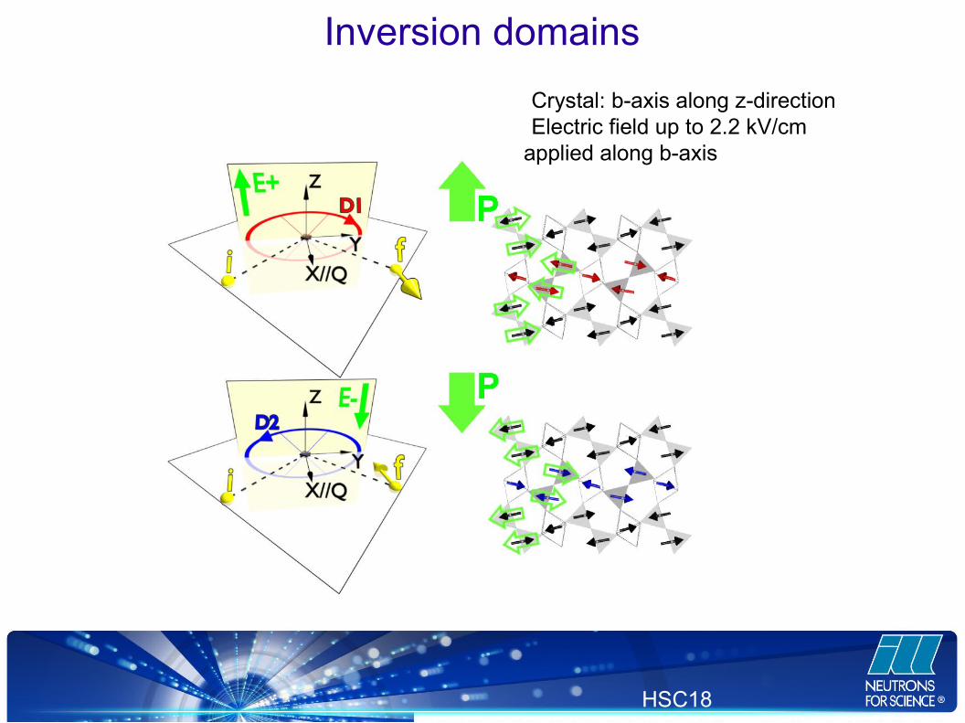
Inversion domains
Crystal: b-axis along z-directionElectric field up to 2.2 kV/cm
applied along b-axis
JDN20—Diffraction , L. Chapon
HSC18
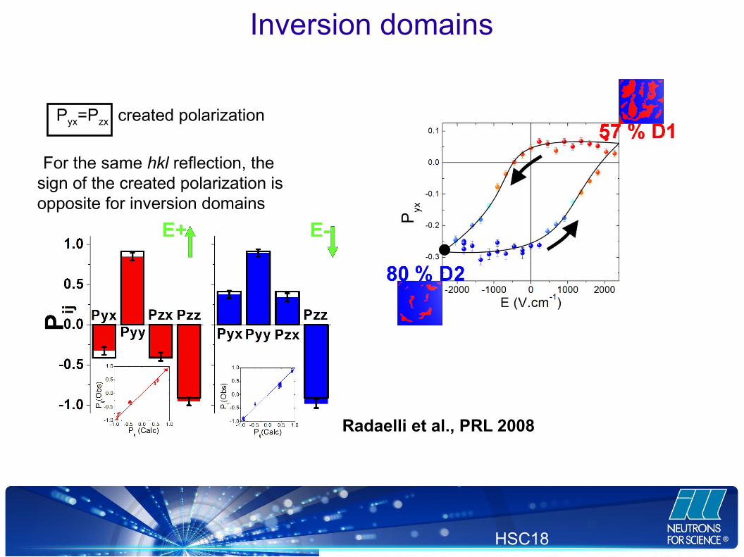
Pyx=Pzx created polarization
For the same hkl reflection, the sign of the created polarization is opposite for inversion domains
Radaelli et al., PRL 2008
Inversion domains

JDN20—Diffraction , L. Chapon
HSC18
Short-range correlations
Probing short-range correlations Via diffuse magnetic scattering
Simple J1-J2 cubic fcc magnet
J2
J1

JDN20—Diffraction , L. Chapon
HSC18
Short range correlations in frustrated beta-Mn
JAM. Paddison et al. PRL (2013)

JDN20—Diffraction , L. Chapon
HSC18
Crystal field excitation(s)
Y. Xiao et al., PRB 88, 214419 (2013)

JDN20—Diffraction , L. Chapon
HSC18
Spin excitations
Martin Mourigal et al., Nature Physics, 9, 435 (2013)