NBER WORKING PAPER SERIES

WHAT DO PARENTS VALUE IN EDUCATION:AN EMPIRICAL INVESTIGATION OF PARENTS’

REVEALED PREFERENCES FOR TEACHERS

Brian A. JacobLars Lefgren

Working Paper 11494http://www.nber.org/papers/w11494

NATIONAL BUREAU OF ECONOMIC RESEARCH1050 Massachusetts Avenue

Cambridge, MA 02138June 2005

We would like to thank Joseph Price and J.D. LaRock for their excellent research assistance. We thankSue Dynarski, Steve Glazerman, Robin Jacob, Larry Katz, Asim Khwaja, Frank McIntyre and seminarparticipants at Stanford University, the Kennedy School of Government, Brigham Young University andthe National Bureau of Economic Research for helpful comments. All remaining errors are our own.Jacob can be contacted at: John F. Kennedy School of Government, Harvard University, 79 JFK Street,Cambridge, MA 02138; email: brian_jacob@harvard.edu. Lefgren can be contacted at: Department ofEconomics, Brigham Young University, 130 Faculty Office Building, Provo, UT 84602-2363; email:l-lefgren@byu.edu. The views expressed herein are those of the author(s) and do not necessarily reflectthe views of the National Bureau of Economic Research.

©2005 by Brian A. Jacob and Lars Lefgren. All rights reserved. Short sections of text, not to exceed twoparagraphs, may be quoted without explicit permission provided that full credit, including © notice, isgiven to the source.

What Do Parents Value in Education? And Empirical Investigation of Parents’ RevealedPreferences for TeachersBrian A. Jacob and Lars LefgrenNBER Working Paper No. 11494July 2005JEL No. I2

ABSTRACT

This paper examines revealed parent preferences for their children's education using a unique

data set that includes the number of parent requests for individual elementary school teachers

along with information on teacher attributes including principal reports of teacher characteristics

that are typically unobservable. We find that, on average, parents strongly prefer teachers that

principals describe as good at promoting student satisfaction and place relatively less value on a

teacher's ability to raise standardized math or reading achievement. These aggregate effects,

however, mask striking differences across family demographics. Families in higher poverty

schools strongly value student achievement and are essentially indifferent to the principal's report

of a teacher's ability to promote student satisfaction. The results are reversed for families in

higher-income schools.

Brian A. JacobJohn F. Kennedy School of GovernmentHarvard University79 JFK StreetCambridge, MA 02138and NBERbrian_jacob@harvard.edu

Lars LefgrenDepartment of EconomicsBrigham Young University130 Faculty Office BuildingProvo, UT 84602-2363l-lefgren@byu.edu

1

I. Introduction

This paper examines parent preferences for their child’s elementary school teacher using

information obtained from principals about parent requests for individual teachers. To our

knowledge, this is the first study to examine the preferences of parents using information on

choices within schools. This allows us to not only control for location and other factors that may

be driving residential or school choice, but also allows us to explore extremely detailed teacher

characteristics. In addition to standard teacher demographics such as gender, experience,

certification status and educational background, we use achievement data to create a value-added

measure of each teacher’s ability to raise student performance. Moreover, we utilize principal

survey information to create teacher measures that reflect “softer” teacher attributes that are

likely to be valued by parents but are typically unobservable to the researcher (e.g., whether the

teacher is adept at classroom management or is perceived as a good role model for students).

We find that, on average, parents strongly prefer teachers that principals describe as best

able to promote student satisfaction, and place relatively less value on a teacher’s ability to raise

standardized math or reading achievement. These aggregate effects, however, mask striking

differences across family demographics. Parents in low-income and minority schools strongly

value student achievement and are essentially indifferent to the principal’s report of a teacher’s

ability to promote student satisfaction. The results are reversed for families in higher-income

and non-minority schools. These results are consistent with a declining marginal utility of basic

math and reading achievement. Moreover, we find that parents in low-income and minority

schools are substantially less likely to request any teacher.

2

Several factors are important to note when interpreting our results. First, our estimates

reflect parent decisions conditional on school choice.1 It is possible that parents may consider

certain factors in choosing a school and other factors in choosing a teacher within a school.

Recent research suggests that the variation in teacher quality within schools is much larger than

the variation in teacher quality across schools (Hanushek et al. 2005). To the extent that parents

recognize this fact, they may well prioritize factors such as proximity to home in choosing a

school, but focus on student achievement in requesting a teacher.

Second, the parameters we estimate reflect both what parents observe and what they

value. To the extent that parents have less information on a particular teacher characteristic, our

estimates may understate parent preferences for this characteristic.2 In particular, one might be

concerned that parents do not have good information on teachers’ ability to raise student

achievement. Parents may have limited access to student test scores by classroom, and even with

such information they may have difficulty inferring teacher quality due to non-random

assignment of students. In practice, however, several pieces of evidence suggest that parents in

this district are able to observe teacher behaviors and attributes associated with student

achievement gains. Most notably, those parents who arguably have the least ability to ascertain a

teacher’s ability to improve student performance – i.e., parents in low-income, high minority

schools – exhibit the strongest preferences for teachers with this quality.3 In addition, this

pattern is evident regardless of whether one uses a principal-reported measure or a teacher value-

1 There is no open enrollment system in this district so that residential location entirely determines elementary school attendance. 2 This does not imply, however, that the parent must observe the actual variable we include in our regressions in order to infer preferences. For example, principal ratings are not observed by the parent but likely reflect the same teacher attributes and behaviors that parents learn about through informal channels. In this case, a significant coefficient on the principal rating suggests that both parents and principals have access to correlated information regarding teacher effectiveness. 3 Of course, one can imagine some circumstances in which parents from wealthier schools are less able to observe teacher quality (e.g., if the variation in teacher quality is smaller in such schools). We explore these alternatives in greater detail below.

3

added measure based on student achievement scores. Indeed, the results are even stronger for

the principal-reported measure, which is likely to reflect teacher behaviors and attributes that are

more easily observable to parents.

Third, the analysis is based on aggregate teacher request data. This limits our ability to

distinguish between the following two cases: (a) parents whose children attend low-income

schools have different preferences than parents whose children attend higher-income schools;

and (b) low-income parents themselves (regardless the school their children attend) have

different preferences than higher-income parents. To the extent that many educational decisions

are made on the basis of school-level characteristics, however, this limitation is less important

from a policy perspective. Finally, because parents are not required to request a teacher, our

estimates reflect the preferences of the roughly 30 percent of parents who make a request.4

While it is of course impossible to know with certainty the preferences of those parents who

made no request, our estimates will reflect the preferences of a particularly interesting and

important group – i.e., those parents who are most involved in their children’s education, and

most likely to be involved in the political process and impact school policy.

Our findings suggest that what parents expect out of school is likely to depend on parent

preferences and family background. To the extent that a child has already learned to read well

by the second or third grade, for example, basic phonics instruction may be unappreciated by the

parent. On the other hand, the parents of a disadvantaged child who is still struggling with basic

literacy are likely to value the emphasis on basic skills. This implies that more and less

advantaged parents may exhibit systematic differences with regards to schooling preferences

even if both sets of parents have the same underlying utility functions.

4 Moreover, to the extent that many parents do not have a strong preference for any particular teacher, but want their children to be in the same classroom, certain teachers preferred by a small number of parents may become focal points. In this case, our estimates may reflect the preferences of a smaller subset of parents.

4

This has important implications for current school reform strategies. First, it suggests

that communities are likely to react quite differently to accountability policies, such as those

embodied in the federal accountability legislation No Child Left Behind (NCLB), depending on

the demographic makeup of the children. Specifically, we would predict that higher-income

communities would express greater dissatisfaction with the achievement emphasis of NCLB.

Second, it suggests that school choice could lead to segregation across demographic groups

driven by the preferences of the parents. At the same time, however, our findings imply that

low-income families who make a request not only recognize high quality teachers, but also

strongly value student achievement. This may alleviate the concerns of some that more

disadvantaged students will not benefit from choice.

While our results cannot be directly compared with the findings from studies that

examine parental choice of schools, our findings suggest that even the best school choice studies

may be more difficult to interpret than previously realized. For example, the preference for

attending racial or socially homogeneous schools that has been documented in prior literature

may not reflect a desire for segregation per se, but instead may reflect an interest in a particular

type of curriculum or pedagogy with the socioeconomic composition of the school merely

serving as a signal of certain practices. For example, low-income families may choose to attend

a school with a high proportion of other low-income families because they believe that the

parents in these schools have preferences that, like their own, prioritize student achievement over

student enjoyment. Conversely, high-income parents may choose to attend schools with high

test scores not because those schools engage in the basic skills and test preparation that is most

helpful for increasing test performance, but for completely opposite reasons – namely, because

the preferences of families in those schools signal that teachers will engage in less basic skills

5

instruction and offer instead a broad curriculum and activities that increase student engagement

in the academic process.

The remainder of the paper proceeds as follows. In Section II, we briefly review the prior

literature on parent preferences in education. In Section III, we describe our data. In Section IV,

we present some preliminary reduced form estimates of the association between teacher

characteristics and parent requests. In Section V, we develop a simple model of parent requests

which we estimate via maximum likelihood to recover the underlying preference parameters of

parents. Section VI concludes.

II. Prior Literature

The prior research on parent preferences falls into several categories. Most prior studies

rely on surveys that directly ask parents what features they value in a school (see, for example,

Lee, Croninger and Smith 1994 and Coldren and Boulton 1991). They find that parents,

including lower-income respondents, highly value academic quality. The two major drawbacks

of these studies are (1) parents may provide socially desirable responses, and (2) surveys do not

present parents with realistic choices that require them to make tradeoffs between specific

characteristics.

A second category of studies examines the actual choices made by parents. In general,

these studies indicate that the location and racial/socioeconomic composition of a school are the

most important factors for parents. For example, Glazerman (1998) utilized an extremely rich

data set to estimate a discrete choice model of parent preferences in the Minneapolis public

school choice program. He found that parents were not more likely to choose schools with high

6

test scores or greater value-added, but instead preferred schools relatively close to home and

ones where they were better represented ethnically and racially.5

Other studies examine the relationship between housing prices and school characteristics

to assess how much parents value different aspects of schooling. In a seminal paper, Black

(1999) examined house prices close to school attendance boundaries within school districts,

thereby removing the influence of neighborhoods, taxes and school spending and focusing

strictly on individual school characteristics. She found that parents were willing to pay 2.5

percent more for a five percent increase in student test scores. Similarly, Figlio and Lucas

(2004) find that arbitrary distinctions embedded in the letter grades that schools receive on state

“report cards” lead to major housing price effects, even after one accounts for underlying school

achievement and other characteristics. Bayer et al. (2003) develop a comprehensive structural

model for identifying preferences for school and neighborhood attributes, and estimate the model

using detailed data from a restricted-use version of the Census. They find that on average

households are willing to pay an additional one percent for homes – substantially lower than in

prior work – when the average performance of the local school is increased by five percent.

While these studies provide an idea of what parents value in their children’s education, they do

not allow one to separately identify which characteristics of schools are valued by parents since

test scores, socioeconomic composition and other factors are very highly correlated.

Finally, several studies approach the question of parental preferences by comparing

schools and students in areas with more or less opportunities for Tiebout choice. Hoxby (1999)

finds that schools in MSAs with more choice offer more challenging curricula, impose stricter

academic requirements and have more structured and discipline-oriented environments,

5 For other examples, see Henig 1990, Lankford and Wyckoff 2000, Weiher and Tedin 2002, Schneider and Buckley 2002.

7

suggesting that parents value these characteristics in schools. Rothstein (2003) explores parental

preferences by examining how the within MSA residential location of families differs across

metropolitan areas, and finds little evidence that parents choose schools for characteristics other

than peer groups.

III. Data

The data for this study come from a mid-size school district located in the western United

States.6 While the students in the district are predominantly white (73 percent), there is a

reasonable degree of heterogeneity in terms of ethnicity and socioeconomic status. Latino

students comprise 21 percent of the elementary population and nearly half of all students in the

district (48 percent) receive free or reduced price lunch. Achievement levels in the district are

almost exactly at the average of the nation (49th percentile on the Stanford Achievement Test).

With the assistance of the district, we were able to collect parental requests for specific

elementary school teachers during the 2003-04 and 2004-05 school years. Unfortunately, the

data on individual students or families was not available in most cases, so our analysis is limited

to aggregate request data (e.g., 15 parents requested Mrs. Smith, 5 parents requested Mr.

Williams, etc.) 7 We discuss the implications of this data limitation in Section IV, using

individual request data we obtained from several schools to examine what type(s) of parents in a

school make requests.

We link these parental requests to administrative files that include a variety of teacher

characteristics such as age, experience, educational attainment, undergraduate and graduate

6 The district has requested to remain anonymous. 7 Data on parent requests is not maintained centrally by the school district. We obtained paper records from individual schools and, with the assistance of school administrators, matched the data to individual teachers, for whom demographic information was available on centralized records.

8

institution attended, and license and certification information. We also link this data to student

achievement and demographic information which allows us to create value-added measures of

teacher effectiveness. Finally, we administered a survey to principals in February 2003 in which

we asked them to evaluate their teachers on a variety of dimensions, providing additional

information about the teachers.

We obtained parent request information for all kindergarten to sixth grade teachers in 11

of the 13 elementary schools in the district in 2003-04 and 2004-05.8 Note that this also includes

a list of all teachers who received zero requests. While we have request information for

kindergarten and first grade teachers, we exclude these from our main analyses since we do not

have value-added or principal-report measures for these teachers. Our final sample thus consists

of 251 teachers.9

The top panel of Table I presents summary statistics for the final sample. Only 14

percent of teachers in our sample are men. The average teacher is 44 years old and has roughly

12 years of experience teaching. The vast majority of teachers attended the main local

university, while 14 percent attended another instate college and 4 percent attended a school out

of state. 16 percent of teachers have a MA degree or higher, and the vast majority of teachers are

licensed in either early childhood education or elementary education. Finally, 10 percent of the

teachers in our sample taught in a mixed-grade classroom and 3 percent were in a “split”

classroom with another teacher.

8 More specifically, we have information for 11 of 13 schools for at least one of the two years, 2003-04 and 2004-05. We have request information from 6 of 13 elementary schools for the 2003-04 academic year and from 10 of 13 elementary schools for the 2004-05 academic year. Parent request data was not available in several schools because teacher requests were not accepted, principals failed to keep a record of such requests, or principals were uncomfortable participating in the research project (this was the case in only 1 of the 13 schools). 9 We will refer to each school-classroom-year observation as a “teacher” although in a small number of cases there were two teachers in the classroom, in which case we use the average characteristics of the teachers.

9

Parent Requests

There is no formal procedure for parent requests in the district. Principals report that they

assign students to classes with an eye toward balancing race, gender and ability across

classrooms within the same grade. Parents submit requests during the spring or summer and

principals make assignments over the summer. During our analysis period, roughly 30 percent

of parents requested a teacher each year and 84 percent of teachers received at least one parental

request. Parents are also able to request that that their child not be placed with a particular

teacher, which we refer to as a negative request. Only about 14 percent of teachers received any

negative requests, and nearly all teachers with negative requests have at least one positive

request as well. Principals report that they are generally able to honor almost all requests and,

perhaps for this reason, parents have an incentive to truthfully reveal their first preference.

Parents in the district appear to have strong and varied preferences for teachers based on

request data. Figure I shows the distribution of positive requests. Among those teachers

receiving at least one request, the average number of requests was 8. The interquartile range of

requests is 7, ranging from the 25th percentile of 3 requests to the 75th percentile of 10 requests.

While these results suggest that parents have strong preferences for particular teachers,

they might also reflect differences in request policies across schools and grades. To explore this

possibility, Figure II plots the distribution of the difference between the most requested and least

requested teacher in each school-grade-year combination. The median difference is 10 and the

90th percentile is extremely large at 19. Even in the 25th percentile, the difference is still 5.

Parent requests also appear to be quite persistent over time, suggesting that they capture

some true teacher characteristic as opposed to simply fads or changing parent preferences.

Figure III illustrates the correlation between requests in 2003-04 and 2004-05. Instead of using

10

the number of requests, we instead use a teacher’s rank within each school-year (i.e., the most

requested teacher receives a 1, the second most requested receives a 2, etc.) to account for any

changes in request policies over time. The correlation is 0.66 and is strongly significant,

suggesting that parents observe something that makes them request the same teachers year after

year.10

Since our analysis will reflect the information and preferences only of those parents who

make requests, it is useful to examine the characteristics of these families. To do so, we regress

the fraction of parents making a positive request in a particular school-year-grade on various

characteristics of the student population. Table II shows the results of these estimates. As

expected, we see that requests are negatively related to the poverty level and minority

concentration. The estimates in column 3, for example, imply that a ten percentage point

increase in the percent of students eligible for free or reduced price lunch in the grade is

associated with 5.2 percentage point fewer parents making a request.11 These results suggest that

the non-financial cost of making a request is higher for parents in low-income, more highly

minority schools. This may be due to language barriers, cultural differences, or information

asymmetries.

Principal Evaluations

To obtain subjective performance assessments, we administered a survey to all

elementary school principals in February 2003 asking them to evaluate their teachers along a

variety of dimensions, including dedication and work ethic, classroom management, parent

10 Figure III is based on the sample of five schools for which we have request data in both 2003 and 2004. 11 Other findings not shown in Table II include: (1) Conditional on student demographics, lagged student ability does not predict parental requests; (2) There is no interaction between student demographics and grade level; (3) All of the results in Table II are robust to a specifications where the dependent variable is the log-odds of parent requests (i.e., ln(p/1-p)). All of these results are available from the authors upon request.

11

satisfaction, positive relationship with administrators and ability to raise math and reading

achievement (see Appendix A for a sample survey form).12 Principals were assured that their

responses would be completely confidential and would not be revealed to the teachers or to any

other school district employee.

The bottom panel of Table I shows the summary statistics of each rating. With an

average rating of roughly 8 on a scale of 1 to 10, it is clear that even these informal and

confidential evaluations are quite lenient. At the same time, Figure IV shows that principal

ratings within each school are approximately normally distributed between 6 and 10 around a

mean of 8, suggesting that the ratings do have considerable variation. While the individual item

ratings are certainly correlated, many of the correlations are far lower than one, suggesting that

the individual items likely reflect multiple teacher attributes (Table A1 shows the full correlation

matrix). To investigate the possibility of several underlying constructs, we conducted an

exploratory factor analysis. Because the principal evaluation of parent satisfaction may be

highly correlated with the parent request measure, we exclude this item from the factor

analysis.13

Table III shows the loadings for the three factors produced by this factor analysis. The

first factor clearly measures student satisfaction, with high loadings on principal ratings of

student satisfaction and teacher as role model. The second factor appears to capture what might

be described as traditional “teaching ability,” with high loadings on classroom management,

12 In this district, principals conduct formal evaluations annually for new teachers and every third year for tenured teachers. However, prior studies have found such formal evaluations suffer from considerable compression with nearly all teachers being rated very highly. These evaluations are also part of a teacher’s personnel file and it was not possible to obtain access to these without permission of the teachers. 13 These factors were derived from a Maximum Likelihood factor analysis method limited to three factors with a Promax rotation. As an additional check, we create a second set of principal measures that are purged of the parent satisfaction information by regressing the factors created above on the parental satisfaction item. We then use the residuals from these regressions as factors that are by construction orthogonal to the principal’s view of parent satisfaction. The results, shown in Table IX, are comparable.

12

organization and ability to influence student math and reading scores. The third factor captures a

teacher’s collegiality, with high loadings on the items that ask principals to assess the teacher’s

relationship with colleagues and administrators.

Student Achievement Measures of Teacher Effectiveness

In this district, elementary students take a set of “Core” exams in reading and math in

grades 1 to 8.14 These multiple-choice criterion-referenced exams cover topics that are closely

linked to the district learning objectives and goals. While student achievement results have not

been directly linked to rewards or sanctions until recently, the results of the Core exams are

distributed to parents and published annually and both teachers and principals pay considerable

attention to the scores.

In order to capture a teacher’s effectiveness, we create value-added measures of each

teacher’s contribution to student performance. Here we present a brief discussion of these

measures. Appendix B provides a more detailed discussion of related identification and

estimation issues.

The primary challenge in constructing consistent estimates of teacher effectiveness using

student achievement data is that students are generally not randomly assigned to classes.

Following the standard practice in this literature, we estimate value-added models that control for

a wide variety of observable student and classroom characteristics including prior achievement

measures and, in some specifications, student fixed effects (see, for example, Aaronson et al.

2004, Rockoff 2004, Hanushek et al. 2005). Specifically, we estimate the following model:

(1) ijkt jt it t k j jt ijkty C X ψ φ δ α ε= Β + Γ + + + + +

14 Students in select grades have recently begun to take a science exam as well. The district also administered the Stanford Achievement Test (a national, norm-referenced exam) to students in grades three, five and eight over this period.

13

where i indexes students, j indexes teachers, k indexes school, and t indexes year. The outcome

measure, y , is a student’s score on a math or reading exam. The scores are reported as the

percentage of items the student answered correctly, which we normalize to be mean zero and

with a standard deviation of one within each year and grade.

The vector X consists of the following student characteristics: age, race, gender, free-

lunch eligibility, special education placement, limited English proficiency status, prior math

achievement, prior reading achievement, and grade fixed effects. C is a vector of classroom

measures that include indicators for class size and average student characteristics. tψ and kφ are

a set of year and school fixed effects respectively. Teacher j’s contribution to student

performance is captured by the 'j sδ . jtα is an error term that is common to all students in

teacher j’s classroom in period t (e.g., adverse testing conditions faced by all students in a

particular class such as a barking dog). ijktε is an error term that takes into account the student’s

idiosyncratic error. In order to properly account for the error structure described above, we

estimate specification (1) using OLS and then correct the standard errors for correlation within

teacher*year using the method suggested by Moulton (1990).15

All of the results presented in this paper are robust to a variety of alternative

specifications of equation (1). Perhaps most importantly, value-added models that include

student fixed effects and time-varying measures of teacher experience yield comparable results

(see Appendix B). The fact that we obtain nearly identical results using value-added measures

that incorporate student fixed effects provides additional reassurance that our measures provide

15 Another possibility would be to use cluster-corrected standard errors. However, such standard errors cannot be computed for teachers that appear in the sample for a single year. Additionally, the estimated standard errors can behave very poorly for teachers that are in the sample for a small number of years.

14

consistent estimates of teacher performance.16 Similarly, we obtain comparable results if we use

a normalized gain score to account for the fact that it may be easier to make achievement gains at

different points in the ability distribution.17

A second concern is that because our value-added measures will be estimated with error

they will suffer from attenuation bias when used as independent variables in a regression. To

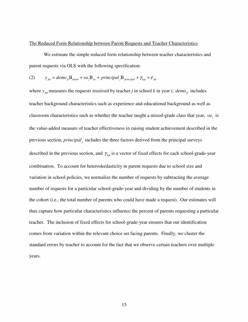
obtain consistent estimates of teacher value-added, we construct empirical Bayes (EB) estimates

of teacher quality which we use in the analysis instead of the estimated value-added measures.

This approach was suggested by Kane and Staiger (2002) for producing efficient estimates of

school quality, but has a long history in the statistics literature (see, for example, Morris, 1983)

and is closely related to the errors-in-variables approach that allows for heteroskedastic

measurement error outlined by Sullivan (2001). Appendix C discusses the statistical properties

of the EB estimates in greater detail.

IV. Empirical Strategy

In this section, we first describe how one can estimate the reduced form relationship

between parent requests and teacher characteristics in an OLS framework. We then explain the

shortcomings of this approach and develop a simple model of parent requests that allows us to

recover the underlying preferences of the parents. 16 We choose not to make these the focal point of the analysis because (1) it would require dropping a small subset of teachers for whom we only observe one year of student achievement data and (2) it is quite difficult to adequately account for estimation error in the value-added in a student fixed effect model. This is due to the fact that because the student fixed effects are imprecisely estimated, the estimation error of the value-added measures has a fairly high correlation across teachers within a specific school. 17 While we make use of extremely rich panel data on student achievement, the value-added specification described above has limitations nonetheless. As Todd and Wolpin (2003) point out, even if one is not concerned about omitted variables (e.g., when students and teachers are randomly assigned to classes), the jδ will generally not

capture the impact of teacher j alone, but will also incorporate the effects of optimizing behavior on the part of families. For example, if a child gets randomly assigned to a poor teacher, her parents may spend more time helping the child with schoolwork or enroll her in an after-school program.

15

The Reduced Form Relationship between Parent Requests and Teacher Characteristics

We estimate the simple reduced form relationship between teacher characteristics and

parent requests via OLS with the following specification:

(2) jkt jt demo j va j principal kgt jkty demo va principal γ ε= Β + Β + Β + +

where jkty measures the requests received by teacher j in school k in year t, jtdemo includes

teacher background characteristics such as experience and educational background as well as

classroom characteristics such as whether the teacher taught a mixed-grade class that year, jva is

the value-added measure of teacher effectiveness in raising student achievement described in the

previous section, jprincipal includes the three factors derived from the principal surveys

described in the previous section, and kgtγ is a vector of fixed effects for each school-grade-year

combination. To account for heteroskedasticity in parent requests due to school size and

variation in school policies, we normalize the number of requests by subtracting the average

number of requests for a particular school-grade-year and dividing by the number of students in

the cohort (i.e., the total number of parents who could have made a request). Our estimates will

thus capture how particular characteristics influence the percent of parents requesting a particular

teacher. The inclusion of fixed effects for school-grade-year ensures that our identification

comes from variation within the relevant choice set facing parents. Finally, we cluster the

standard errors by teacher to account for the fact that we observe certain teachers over multiple

years.

16

A Structural Model of Parent Preferences for Teachers

While the reduced form approach described above is attractive in its simplicity, it has

several important limitations. First, the reduced form estimates do not account for the fact that a

teacher’s market share of parent requests is likely to respond differently to teacher quality based

on the number of teacher choices available. In a highly fragmented market, for example, we

might expect a marginal change in teacher quality to have a smaller absolute effect on that

teacher’s share than in a market with only two options. Thus, while the OLS coefficients may

yield a good approximation to the average effect of a particular characteristic on the market

share, they may well perform poorly when examining grades with more or fewer teacher options

than average. In addition, the reduced form strategy fails to take into account that the sum of the

market shares (including the no request option) must necessarily lie between zero and one, which

is likely to result in reduced statistical efficiency and predicted market shares that fall outside the

interval between zero and one. Given our limited sample size, this is an important consideration.

Perhaps most importantly, the reduced form model does not allow one examine how

parent preferences or the cost of making a request vary across demographic groups. This is

because the costs of making a request will affect both the average number of requests as well as

the relationship between requests and teacher attributes. For example, if the cost of making

requests is high for low-income families, we would expect these families to make few requests

and to be less responsive to any particular teacher characteristic. In this case, the reduced form

coefficient of the interaction between parent income level and a teacher characteristic will reflect

both preferences for the characteristic as well as the cost of making a request. A structural model

will allow us to separately identify these factors.

17

While the approach we outline below is very similar to a typical conditional logit discrete

choice model, it differs from the standard model in several ways owing to the nature of the

choice problem we study and the data we utilize. In particular, our estimation method must

account for the fact that (1) we only have aggregate counts of parent requests rather than parent

level request information, (2) the number of choice options varies across individuals depending

on how many classes are offered in a particular school-grade-year, and (3) the expected teacher

quality associated with making no request must be modeled as a function of the quality of all

teachers in the choice set.18

We begin by assuming that the quality, ,j sq , of teacher j in school*grade s is a linear

function of observed (by both us and the parents) teacher characteristics ,j sX :

(3) , ,j s j sq X β= .

In our case, the vector X includes teacher demographics such as education and experience, value-

added measures, and principal-reported evaluations of the teacher, which reflect typically

unobservable (to the econometrician) teacher attributes.

We next assume that there is some cost of making a request,

(4) s sc Z γ= ,

where Z includes school and grade level covariates sZ .19 In our baseline specification, we

assume that the cost of making a request is a function of the child’s grade and school (i.e., the

18 In these respects, our approach is related to a larger industrial organization literature on the estimation of preference parameters and demand elasticities based on aggregate market shares and distributions of consumer characteristics (see, for example, Berry, Levinsohn, and Pakes, 1995). The model we develop is similar to the Berry-Levinsohn-Pakes (BLP) models common in IO, but is simpler than many recent applications of BLP-type models which incorporate additional complexity in an effort to calculate reasonable own and cross-price elasticities of demand. Because the current paper doesn’t examine these issues, we use a simpler framework. 19 With individual data, we would of course have the cost be a function of student or parent characteristics. This is not generally possible with the data available to us.

18

vector Z will include a set of grade fixed effects and school fixed effects).20 This assumption is

motivated by the possibility that school administrators may have different informal policies

regarding requests, and that requests may be more or less acceptable for children of different

ages.21

The utility parent, i, receives from requesting teacher j is given by that teacher’s quality,

minus some cost, sc , plus an idiosyncratic utility component, ijsε , that captures the idiosyncratic

match quality between the teacher and the child. Assuming that every parent request is granted

and that parent utility is linear in quality and cost, we can write the utility associated with parent

i requesting teacher j as:

(5) , , , , ,i j s j s s i j sU X Zβ γ ε= − + .

We will assume that this utility component is i.i.d. from a type 1 extreme value distribution.22

If a parent makes no request, we will impose that the expected teacher equals the average

teacher quality in the parent’s choice set. Essentially, we assume that parents believe that if they

make no request their child has an equal probability of being assigned to any teacher in the

choice set. Hence, the utility associated with no request equals the average teacher quality (not

including the idiosyncratic match components) plus a type 1 extreme value disturbance, noε , that

can be interpreted as the idiosyncratic utility benefit of not making a request.23

20 In Table VIII, we show that our results are robust to including school-grade-year fixed effects in the cost function. 21 Note that the grade and school fixed effects in the cost equation implicitly capture much of the impact of family demographics on the average number of requests. In our baseline specification, we do not include separate measures of family demographics. However, we explicitly examine the role of family demographics in the subsequent models discussed below. 22 The c.d.f. of this distribution is given by ( )( ), ,

, ,( ) exp i j s

i j sF e ε µε − −= − , where µ is a location parameter. The mean

of the idiosynctratic utility term equals .5772µ + . This mean is not identified since it affects the utility of all

options symmetrically. Thus, one can assume that ijsε is mean zero without loss of generality. 23 In addition to the idiosyncratic utility associated with each teacher, there is also an idiosyncratic cost associated with making any request. One can think of the negative of this cost as the idiosyncratic benefit of not making a request. Since what matters is not the level of utility of each choice but rather the difference in utility between any

19

(6) 1, ,( _ )

K

ksk

is i no s

XU no request

K

βε== +

�,

where K is the number of teachers in the choice set.24

Of course, it is possible that sophisticated parents may recognize that their child is less

likely to be assigned to a popular teacher if the parent does not submit a request. In Table IX, we

show that our results are robust to changing this aspect of the model, and instead assuming that

the expected teacher quality equals the weighted average of teacher quality in the parent’s choice

set where the weights correspond to the number of vacancies in a teacher’s class. For example,

if one of three teachers in a particular grade is always oversubscribed and the other two teachers

receive an equal number of requests, then a parent who does not make a request will expect his

or her child to receive the average quality of the two less popular teachers.

If each parent chooses whichever alternative yields the highest utility, a teacher’s

expected market share and the probability that any given family selects teacher j is given by:25

(7) ( ) ( ) ( )

( )

,,

,1

,1

expPr

exp exp

j s sj s K

k s Kk

j s sk

X ZE share request j

XX Z

K

β γ

ββ γ=

=

−= = =

� �� �� �+ −� �� �� �

��

.

The no request share is:

two choices, it is irrelevant whether the idiosyncratic cost of making a request is included in the “no request” option or in every teacher request option. 24 This framework imposes that the idiosyncratic utility terms for teachers average to zero within each choice set for each parent. Because the mean of the idiosyncratic utility terms is not identified, one can assume that it equals zero without loss of generality. Imposing that these idiosyncratic terms average to zero within a finite sample is a stronger assumption. 25 See McFadden (1973) for a proof.

20

(8) ( ) ( )

( )

,1

,

,1

,1

exp

Pr

exp exp

K

k sk

no s K

k s Kk

j s sk

X

K

E share request noX

X ZK

β

ββ γ

=

=

=

� �� �� �� �� �� �= = =

� �� �� �+ −� �� �� �

�

��

.

Given the assumptions above, the probability that we observe a particular distribution of requests

in a grade is given by:

(9) ( )

( ) ( ) ( )1 2

1 1 2 2Pr , ,..,

Pr 1 Pr 2 ... Pr no

no no

n n n

num n num n num n

A t t t no

= = = =

= = =,

where inum is a variable corresponding to the number of parents selecting teacher i, in is the

particular realization of this variable, and A is a constant that forms part of the multinomial

distributions and simply shows the number of different ways in which a particular combination

of teachers could be selected. This constant varies on the basis of the number of choices

available and the aggregate counts we observe. Because it is not a function of the probabilities

themselves, we can ignore it for the purposes of estimation.

It is then straightforward to identify the preference and cost parameters using maximum

likelihood. Using equation (9), we can find the probability of observing a particular set of

aggregate choices in each grade*school*year combination. Note that these probabilities are a

function of preference and cost parameters of our model. We then multiply the probabilities for

each grade-school-year combination to determine the probability of observing the entire set of

aggregate choices that we find in the data. This product gives us our likelihood function and

allows us to estimate the model.

21

To this point, we have assumed that the idiosyncratic error terms are independent within

each choice set. This is unlikely to be the case as teachers differ in both observable and

unobservable ways. Because of this, the estimation method may yield standard errors that are

significantly understated. Furthermore, some teachers appear in multiple years in our dataset,

further complicating statistical inference. To address these problems, we bootstrap the standard

errors, clustering at the school-grade level. This takes into account unobserved systematic

differences across teachers as well as persistence in unobserved teacher quality.26

While we do not know which parents made each request, we can take advantage of the

aggregate demographic information we have for each grade-school-year combination to estimate

the differences in costs and preferences across different types of individuals. This approach has

been used extensively in the industrial organization literature to estimate preference parameters

and demand elasticities based on aggregate market shares and distributions of consumer

characteristics (see, for example, Berry, Levinsohn, and Pakes, 1995). The intuition is that by

examining how the relationship between teacher characteristics and requests changes with the

fraction of, for example, low-income families in the grade, we can identify how the structural

parameters vary with income.

More specifically, suppose we have two types of families, l and h. Each type has

different parameters for both their utility and cost functions. If this is true, the expected market

share of teacher j will equal:

26 To the extent that teachers change grades across years, the clustering procedure may not fully account for the non-independence of the utility terms across years for a specific teacher. Fortunately, nearly all teachers teach the same grade in all years.

22

(10)

( ) ( )

( )

( ) ( )

( )

,,

,1

,1

,

,1

,1

exp

exp exp

exp1

exp exp

j s h s hhj s s K

k s h Kk

j s h s hk

j s l s lhs K

k s l Kk

j s l s lk

X ZE share

XX Z

K

X Z

XX Z

K

β γω

ββ γ

β γω

ββ γ

=

=

=

=

−=

� �� �� �+ −� �� �� �

−+ −

� �� �� �+ −� �� �� �

��

��

,

where the subscripts denote the type of family making the request and hsω represents the share of

type h families within the school*grade, s. Though theoretically, we could identify how school

and grade affected the cost of making a request separately for families in each of the two groups,

in practice there is insufficient variation in family demographics across grades within a school to

do so. For this reason, we will constrain the school and grade fixed effects to the same for each

group. We will allow the cost of making a request to vary only by a constant across groups.

Even this parameter will be estimated with insufficient precision to draw strong conclusions,

however.

While the model described above captures many of the essential features of the parent

request decision, it does have several limitations. First, we assume that all requests are honored.

While this is not strictly true, our discussions with principals suggest that the vast majority of

requests are granted so this assumption is unlikely to affect the main conclusions of our analysis.

Second, as is the case in all conditional logit models, our assumption of independent errors

implies an assumption regarding the Independence of Irrelevant Alternatives (IIA). In settings

where certain choices are thought to be extremely good substitutes for each other (e.g., a red bus

and a blue bus), this assumption is particularly unrealistic. To the extent that teachers are

23

unlikely to be close substitutes to each other, this assumption is less problematic.27 Moreover,

while the IIA assumption is particularly problematic for predicting market shares, it does not

necessarily introduce substantial bias into parameter estimates (Glazerman 1998).

Limitations of Using Aggregate Request Data

While the use of aggregate data will not affect our inferences regarding the average

preference parameters in the population, it does limit our ability to examine variation in parent

preferences across individual demographic characteristics.28 Ideally, in order to identify how

family preferences vary with demographics, one would interact characteristics of the requested

teacher with characteristics of the requesting parent. As explained above, it is possible to

leverage information regarding the distribution of demographic characteristics across school-

grade-years to examine these interactions. This approach has two limitations, however. First,

because we use aggregate data, we know the characteristics of a requesting parent only

probabilistically. This reduces the efficiency of the resulting parameter estimates. Second,

aggregate data limits our ability to distinguish between the following cases: (a) parents whose

children attend low-income schools have different preferences than parents whose children

attend higher-income schools; and (b) low-income parents themselves (regardless the school

their children attend) have different preferences than higher-income parents.29 To the extent that

27 In the industrial organization literature, researchers are particularly concerned with this aspect of the discrete choice models. If a consumer’s utility function is simply composed of a small number of observable components and an independent error, then as the price of a good rises the model predicts substitution towards other popular products regardless of their similarity to the original product. Berry, Levinsohn and Pakes (1995) propose a model with random coefficients in the utility function. This type of model predicts that as the price of one good rises, consumers will substitute toward other goods with similar observable characteristics. 28 To see this, note that the teacher is the relevant unit of observation in our analysis. Assuming that we have not omitted any important teacher characteristics and the functional form of the included covariates is correct, our estimates will be unbiased. 29 More generally, if one uses aggregate data, there is a choice of two identifying assumptions with regard to estimating the relationship between demographics and preferences. First, one can assume that unobserved

24

many educational policy decisions are made at the school level, however, this limitation may not

be particularly important from a practical standpoint.30

V. Results

Having outlined our estimation strategy, we will now present and discuss our findings.

We begin by presenting OLS estimates of the relationship between parent requests and teacher

characteristics, but quickly move to the structural estimates described above. A more extensive

set of OLS results, that includes interactions between family demographics and parent choices, is

presented in Appendix D. All of the results from the OLS models are consistent with the main

structural estimates presented here.

Reduced Form Estimates

Table IV presents the estimates from equation (2) where the outcome measure is the

normalized number of positive requests for each teacher.31 Column 1 focuses teacher

demographics and aspects of classroom organization. We observe that more experienced receive

more requests than first year teachers or teachers who are new to the school. Interestingly, we

preferences for teacher characteristics are not systematically correlated to neighborhood demographics. This would be true if, for example, families were randomly assigned to neighborhoods. In this case, the method we describe above will perfectly identify the average preferences of high-income (non-minority) and low-income (minority) families. An alternative assumption is that there exists perfect Teibout sorting to neighborhoods on the basis of preferences for educational outputs. In this case, all families within a school have the same preferences and average demographics are simply a proxy for what one might describe as community values. Under this assumption, one can use aggregate data to observe how community preferences vary with average demographics. Of course, the truth is likely to be some combination of these two extremes and without individual-level data, one cannot test between them. 30 In addition, the use of aggregate requires that we assume that families within a particular demographic group are homogenous (except for idiosyncratic preference and cost shocks). It is possible, however, that non-free lunch children in a disadvantaged school differ systematically from non-free lunch children in a wealthy school. To the extent that this is true, our estimates of the differences in preferences and costs between different groups may be overstated. They will, however, have the correct sign and show approximate differences in the parameters of interest. 31 Specifications that incorporate information on negative requests yield comparable results (see Table IX).

25

also find some evidence that parents have preferences regarding certain aspects of classroom

organization. For example, parents appear to dislike mixed-grade classrooms, which are

generally created when there are not enough children enrolled in a particular grade level to

justify a new class composed entirely of students from that grade. In fact, teachers in these

mixed-grade classrooms receive 7 percentage points fewer requests than their colleagues. This is

consistent with the evidence that mixed-grade classrooms reduce student achievement (see Sims,

2005). Principals in the district indicate teachers in these classrooms often teach one grade and

ask a teacher’s aide to teach the other grade, particularly in subjects such as math and science

where the material varies across grades and teaching a heterogeneous ability group is difficult.

To the extent that parents are aware of this arrangement, one can easily imagine why such

classes are unpopular.

In column 2, we show the relationship between teacher value-added and parent requests.

The point estimate indicates that teachers with higher value-added measures receive more

requests. While the estimates are not significant, the magnitude implies that a one standard

deviation increase in teacher value-added is associated with roughly 1.2 percentage points more

parent requests. Given that the average teacher receives requests from roughly 9.2 percent of

parents, this reflects a 13 percent effect. In column 3, we see that parents are significantly more

likely to request teachers who principals rate highly in terms of raising student achievement.

Indeed, a one standard deviation increase in a teacher’s achievement rating is associated with a

4.2 percentage point (45 percent) increase in parent requests. Column 4 shows that parents also

place an extremely high value on the ability of teachers to make their children happy. A one

standard deviation increase in the student satisfaction rating is associated with a 5.5 percentage

point (53 percent) increase in parent requests.

26

The specification in column 5 includes all of the principal measures together with the

estimated value-added. We see that the parent satisfaction measure is more highly correlated

with parent requests than the achievement measure. In addition, the principal achievement

measure is more strongly related to parental requests than the value-added measure, which

indicates either that parents prefer the qualities captured in the principal measure more than the

value-added measure or that parents can more easily observe the qualities identified by the

principal. To the extent that the principal measure includes factors such as classroom

organization and management, the later explanation seems compelling. 32 In column 6, we show

results from a specification in which we include teacher demographics, value-added measures,

and the principal evaluation factors. The results are substantively the same, though the

coefficients on a number of the teacher demographic variables have fallen in magnitude.

Column 7 of Table IV shows the estimates of the teacher quality parameters from our

structural model. The average marginal effects of each attribute, shown in the square brackets,

are computed by calculating the marginal effect for each individual and averaging across all

observations. We see that the structural model produces results quite similar to the reduced form

approach. Most importantly, the relationship between parent requests and teacher attributes that

capture educational outputs such as student achievement and satisfaction remains strong.

32 Interestingly, we also see that teachers who the principal rates as better able to get along with colleagues receive fewer requests from parents. This is consistent with principals providing systematically biased evaluations of teacher attributes. Suppose, for example, that conditional on actual ability to raise standardized test scores a principal gives higher evaluations to teachers she likes. In this case, we expect that between two teachers with the same principal-rated instructional ability, the better-liked teacher will be less effective at raising student achievement. Jacob and Lefgren (2005) explore this issue in greater detail.

27

Main Structural Estimates

Having established the baseline results for the structural model, we now turn to the

interaction between demographics and parent preferences. For the reasons mentioned earlier, we

focus on the coefficients from our structural model. We allow the preference parameters to vary

arbitrarily across group and allow the cost of making a request to vary across demographic

groups, grades and schools. Doing so allows the probability of selecting a particular teacher to

vary arbitrarily with the demographic makeup of the class. The demographic characteristics we

consider include the child’s eligibility for free or reduced price lunch, ethnic/racial classification,

and prior achievement level. For the sake of parsimony, the models described below limit the

teacher characteristics to covariates that reflect two critical education outputs – student

achievement and student satisfaction – though we obtain comparable results from models that

include additional teacher characteristics (see Table IX).33

To provide a basis for comparison, the first column in Table V shows estimates where the

preference and cost parameters do not vary across groups. As before, we find that parents have a

strong preference for teachers who promote student satisfaction and a relatively weak but

statistically significant preference for teachers who promote student achievement. Specifically, a

one standard deviation increase in the student satisfaction measure will result in a teacher

receiving 3.9 percentage points (42 percent) more requests whereas a one standard deviation

increase in the student achievement measure will result in a teacher receiving 1.5 percentage

points (16 percent) more requests.

33 Of course, it is possible to examine whether preferences for other teacher characteristics such as experience or gender vary with family demographics. However, it is difficult to interpret these results because it is unclear what educational outputs these characteristics may capture, and whether this would be consistent across demographic group.

28

Columns 2-10 in Table V come from specifications that allow the preferences parameters

to vary by family demographics. Assuming that all parents can observe teacher behaviors and

attributes that are correlated with these characteristics, the estimates thus reflect the preferences

of different groups of parents. It appears that families who are not eligible for free lunch

strongly value parent satisfaction and are essentially indifferent to the principal’s report of a

teacher’s ability to increase student achievement. The situation is reversed for the parents of

children who are eligible for free lunch. These results are highly significant.

These results are echoed when we examine the preferences of minority and non-minority

families. In particular, minority families value a teacher’s ability to increase achievement while

non-minority families appear to care only about student satisfaction. The same picture emerges

when we look at the requests of parents whose students are in the top and bottom half of the

initial achievement distribution.34 In all three comparisons, the differences in the preference for

student satisfaction are significant at the 5 percent level; the differences in the preference for

principal-reported achievement factor are generally significant at the 10 percent level or better.

To examine the robustness of this result, Table VI presents estimates from models that

include the principal measure of student satisfaction, but replace the principal measure of a

teacher’s effectiveness at raising student achievement with our value-added measure of teacher

effectiveness. The results are comparable to those presented above. That is, low-income and

minority parents care more about student achievement and much less about student satisfaction

while higher-income and non-minority parents have the opposite preferences.

34 As noted earlier, we use test scores from the prior year to determine the percent of students scoring in the top half of the district distribution in a school-grade-year. Because we do not have student test scores for the 2003-04 school year, we use test scores for the 2002-03 school year to calculate the prior ability of the cohorts entering in 2004-05. Unfortunately, we do not have first grade test scores for 2002-03. For this reason, we must exclude second grade classes in both 2003-04 and 2004-05 and third grade classes in 2004-05 from the analyses shown in columns 8-10 (in both Table VII-A and VII-B). This is one reason that the reduced precision of these results.

29

The fact that parents of disadvantaged children appear to care about a teacher’s ability to

increase achievement more than student satisfaction is consistent with a decreasing marginal

utility of student achievement. If all parents have a strictly concave function defined over

student achievement and student happiness, to the extent that high-income and non-minority

parents have children with a higher baseline level of achievement, we expect that on the margin

child happiness will be more valued than further achievement gains in school.

Sensitivity Analyses

The results presented above suggest that parents in lower vs. higher-income schools have

quite different preferences for their children’s education. In this section, we explore the

robustness of this finding.

First, one might be concerned that the level or variance of teacher quality differs

substantially across schools and is associated with family demographics in a way that raises

doubt about the interpretation presented here. For example, it may be that the average teacher’s

ability to raise student achievement is sufficiently high in advantaged schools that parents do not

need to focus on student achievement. Similarly, one might speculate that there is so little

variance in the teacher achievement measures in higher-income schools that parents believe that

all teachers are effectively equal along this dimension and thus not place any weight on it in

choosing a teacher. Both stories would explain the pattern of results we find without implying

differential preferences for achievement.

In order to explore this possibility, we regress various measures of teacher quality on the

percentage of students in a particular school-grade-year who are eligible for free-lunch.35 The

results are presented in Table VII. All standard errors are clustered at the school level. Because 35 The results are similar for the percentage of minority students and the average lagged achievement measure.

30

the principal factors are created by first normalizing the principal survey items to mean zero and

standard deviation one within school, it is not useful to compare the principal factors across

schools. We therefore focus on “raw” principal responses (measured on a scale of 1-10) for

several key survey items.36

Columns 1-4 examine the level of various teacher characteristics. The F-statistics on

models that include only school fixed effects (shown in the bottom row of the table) confirm that

the level of teacher quality varies significantly across schools. However, this variation does not

appear to be associated with student poverty. The estimates on percent eligible for free-lunch

indicate that there is no significant relationship between school poverty level and teacher value-

added or principal reported measures of teacher quality.37 The dependent variable in columns 5-

8 is the range of a particular principal rating within the relevant choice set (i.e., the

school*grade*year). The results indicate that the range of principal ratings is smaller in school-

grade-years with a higher percentage of students who are eligible for free-lunch.

A second concern involves the use of aggregate data. To the extent that minority or low-

income parents never (or very rarely) make a request, observed differences in preferences across

schools cannot reflect preference variation related to a child’s own free lunch status. To explore

this possibility, Table VIII presents information on individual parent requests we were able to

obtain from two schools.38 The first column shows the average demographic characteristics in

the district in 2002-03 to provide a baseline from which to assess the two schools we examine.

These two schools are roughly at the 25th and 75th percentiles of the distribution in terms of free

36 Of course, differences in principal ratings across schools may result from differences in how harshly principals rate their teachers. 37 See Appendix B for more detailed discussion of how the value-added measures are calculated. 38 For reasons of convenience, these two principals preferred to give us a spreadsheet with individual requests as opposed to the aggregated requests. In terms of request policies and request rates, they are similar to other schools in the district.

31

lunch eligibility, and thus provide a snapshot which is likely to generalize to the broader sample

of schools. Columns 2 and 4 show the demographic composition of the students in these

schools; columns 3 and 5 show the composition of students who made requests in these schools.

In both schools we see that the students who make requests are more likely to be white and less

likely to be eligible for free lunch than the average student in the school. This confirms our

earlier findings that free lunch and minority status are associated with increased costs of making

a request. However, we also see that a non-trivial percent of requests come from families who

are Hispanic, do not speak English as a first language and/or are eligible for free lunch This

lends credence to our interpretation that the findings reflect differences in preferences between

observably different groups of parents within a school.

Finally, Table IX examines a variety of alternative specifications in order to test the

robustness of our results. For the sake of simplicity, we only present estimates for free-lunch

eligibility. Other results are available on request. The first row presents the baseline estimates

taken from columns 2 and 3 of Table VI. In this baseline specification, the cost of making a

request was modeled as a function of grade fixed effects, school fixed effects and the

demographic characteristic (i.e., free lunch eligibility). In row 2, we allow the cost function to

vary only with grade and the demographic characteristic. The results are substantively the same,

though the significance of some coefficients is reduced. In row 3, we allow the cost function to

vary by grade*school*year, yielding estimates similar to the baseline. The next set of results

examines alternative specifications of the preference parameters. In the baseline model, parent

preferences are modeled as function of two key outputs – the teacher’s ability to promote student

achievement and student satisfaction (both principal-reported). Row 4 includes the principal-

reported teacher collegiality measure; row 5 includes a several teacher demographics as well as

32

the collegiality factor. The results for both specifications are comparable to the baseline. Row 6

presents estimates of a model where the outcome measure includes negative as well as positive

request information. More specifically, we apportion each negative request to the other teachers

in the school-grade-year in proportion to the number of positive requests these teachers received.

Our results remain the same. Row 7 shows the results of a model that uses alternative principal

measures. Recall that the student achievement and satisfaction factors used in the baseline

analysis were created from a factor analysis that included all of the individual principal items

except the principal report of parent satisfaction. We excluded this item because of concerns that

it is highly influenced by parent requests, which introduces a simultaneity problem into the

model and may bias our estimates. As a further guard against this simultaneity problem, we

regress the original factors on the principal satisfaction item on use the residual from the

regression as an alternative principal measure of a teacher’s ability to raise student achievement

and promote student satisfaction. These residual factors are, by construction, orthogonal to a

principal’s evaluation of a teacher’s ability to promote parent satisfaction. As we see from the

estimates in row 7, the estimates using these alternative measures yield very similar results,

though there is a decrease in the precision of the estimates. Finally, in row 8 we assume that the

expected teacher quality associated with making no request is a weighted average of teacher

quality where the weights correspond to the number of vacancies in each class. This is

consistent with a model in which parents are fully rational and have perfect information. Again,

the results are virtually identical to the baseline.

33

VI. Conclusions

In this paper, we examine the parents’ revealed preferences for their child’s schooling.

We find that on average parents strongly prefer teachers that principals describe as the most

popular with students, and place relatively less value on a teacher’s ability to raise standardized

math or reading achievement. These aggregate effects, however, mask striking differences

across family demographics. Low-income and minority families strongly value student

achievement and are essentially indifferent to the principal’s report of a teacher’s ability to

promote student satisfaction. The results are reversed for higher-income and non-minority

families.

Our findings suggest that what parents want from school is likely to depend on family

circumstances as well as parent preferences. Thus, we might expect advantaged and

disadvantaged parents to exhibit systematic differences with regards particular educational

policies or programs even if both sets of parents have the same underlying utility functions. This

has important implications for current school reform strategies. For example, it suggests that

communities are likely to react quite differently to accountability policies, such as those

embodied in No Child Left Behind. It also suggests that school choice could lead to segregation

across demographic groups driven by the preferences of the parents. At the same time, however,

our findings imply that low-income families are not only able to recognize high quality teachers,

but also strongly value student achievement. This result belies the concern that school choice

programs will not benefit poor children because their parents will not fully recognize or

sufficiently value academic achievement. Finally, our analysis suggests the results of prior

school choice studies may be considerably more difficult to interpret than previously realized. In

34

particular, the preference for attending racial or socially homogeneous schools that has been

documented in prior literature may not reflect a desire for segregation per se, but instead may

reflect an interest in a particular type of curriculum or pedagogy with the socioeconomic

composition of the school merely serving as a signal of certain practices.

35

References

Aaronson, Daniel, Lisa Barrow and William Sander (2002). “Teachers and student achievement

in the Chicago public high schools.” Working Paper Series WP-02-28, Federal Reserve Bank of Chicago

Bayer, Patrick, Fernando Ferreira, and Robert McMillan, “A Unified Framework for Measuring

Preferences for Schools and Neighborhoods.” Working paper.

Berry, Steven, Levinsohn, James and Pakes, Ariel (1995). “Automobile Prices in Market Equilibrium.” Econometrica 63(4): 841-890.

Black, Sandra E., “Do Better Schools Matter? Parental Valuation of Elementary Education,” The

Quarterly Journal of Economics (May 1999). Coldren, J. and Boulton, P. (1991). “Happiness as a criterion of parents’ choice of school.”

Journal of Education Policy 6(2): 169-178. Figlio, David N. and Maurice E. Lucas (2004). “What’s in a Grade? School Report Cards and

the Housing Market.” American Economic Review. 94(3): 951-604. Glazerman, Steven (1998). “Determinants and Consequences of Parental School Choice,”

Doctoral Dissertation. University of Chicago, Harris School of Public Policy. Hanushek, Eric A., John Kain, Daniel M. O’Brien and Steven G. Rivkin (2005). “The Market

for Teacher Quality.” NBER Working Paper #11154. Jacob, Brian A. (2005). “Accountability, incentives and behavior: the impact of high-stakes

testing in the Chicago public schools. Journal of Public Economics. Jacob, Brian A. and Lars Lefgren (2005). “What Do Parents Value in Education? An Empirical

Investigation of Parents’ Revealed Preferences for Teachers.” Working paper. Jacob, Brian A. and Stephen D. Levitt (2003). “Rotten apples: an investigation of the prevalence

and predictors of teacher cheating.” Quarterly Journal of Economics CXVIII(3): 843-878 Henig, Jeffrey R. (1990). “Choice in Public Schools: An Analysis of Transfer Requests in

Magnet Schools.” Social Science Quarterly. 71(1): 69-82. Hoxby, Caroline, “The Effects of School Choice on Curriculum and Atmosphere,” in Paul E.

Peterson and Susan Mayer (eds.), Earning and Learning: When Schools Matter, Washington, DC: Brookings Institution Press (1999), pp. 281-316.

Kane, Thomas J. and Douglas O. Staiger (2001). Volatility in School Test Scores: Implications

for Test-Based Accountability Systems. UCLA Graduate School of Public Policy Studies, Working paper.

36

Lankford, Hamilton and James Wyckoff, “The Effect of School Choice and Residential Location

on the Racial Segregation of Students,” unpublished paper, State University of New York-Albany (October 2000), http://www.albany.edu/~wyckoff/segpapr14.PDF

Lee, V.E. , Croninger, R.G. and Smith J.B. (1994). “Parental choice of schools and social

stratification in education: The paradox of Detroit.” Educational Evaluation and Policy Analysis 16(4): 434-457.

McFadden, Daniel (1973). “Conditional Logit Analysis of Qualitative Choice Behavior.” In P.

Zarembka, ed., Frontiers in Econometrics. New York: Academic Press. Morris, Carl N. (1983). “Parametric empirical Bayes inference: theory and applications.”

Journal of the American Statistical Association 78(381): 47-55. Rockoff, Jonah E. (2004). “The impact of individual teachers on student achievement: evidence

from panel data.” American Economic Review 94(2): 247-252. Rothstein, Jesse, “Good Principals or Good Peers: Parental Valuation of School Characteristics,

Tiebout equilibrium, and the Incentive Effects of Competition Among Jurisdictions,” Working Paper #3, Princeton University, Education Research Section (2003).

Schneider, Mark, and Jack Buckley, “What Do Parents Want From Schools? Evidence from the

Internet,” Educational Evaluation and Policy Analysis, 24 n. 2 (2002), 133-144. Sims (2005). “How Flexible is Education Production? Combination Classes vs. Class Size.”

Working Paper, Brigham Young University. Sullivan, Daniel G. (2001). “A note on the estimation of regression models with heteroskedastic

measurement errors.” Working paper 2001-23. Federal Reserve Bank of Chicago. Weiher, Gregory R. and Kent L. Tedin (2002). “Does Choice Lead to Racially Distinctive

Schools? Charter Schools and Household Preferences.” Journal of Policy Analysis and Management, 21(1): 79-92.

37

Appendix A: Sample Principal Survey Form We thank you for agreeing to answer the questions in this survey. By answering this survey, you will aid in determining what aspects of teacher effectiveness are most important for students, parents, and principals. Your responses to these surveys will be completely confidential. They will never be revealed to any teachers, administrators, parents, or students. Only statistical averages and correlations will be presented in reports for the district and possible publication in an academic journal. We will now ask you to rate teachers on the basis of a number of different performance criteria. Please use the following descriptions in rating teachers on a scale of 1 to 10. 1-2: Inadequate – The teacher performs substantially below minimal standards in this area. 3-5: Adequate – The teacher meets minimal standards (but could make substantial improvements in this area). 6-8: Very good – The teacher is highly effective in this area. 9-10: Exceptional – The teacher is among the best I have ever seen in this area (e.g., in the top 1% of teachers).

Part I: Teacher Ratings Teacher Characteristic Teacher 1 Teacher 2 Teacher 3 Teacher 4 Teacher 5

Dedication and work ethic

Organization

Classroom management

Raising student math achievement

Raising student reading achievement

Role model for students

Student satisfaction with teacher

Parent satisfaction with teacher

Positive relationship with colleagues

Positive relationship with administrators

Overall teacher effectiveness

How many years have you worked with this teacher (in your current school or another school)?

How many years has this individual been teaching (in your school or another)? Please give your best guess if you are not certain.

38

TABLE A-1 CORRELATION MATRIX OF PRINCIPAL RATING ITEMS

Dedication and Work Ethic

Organization

Classroom

Management

Math Reading Role Model

Stud. Satisfacti

on

Parent Satisfacti

on

Positive relationship with

colleagues

Positive relationship with admin

Overall

Dedication and work ethic 1.00

Organization 0.595 1.00

Classroom management 0.517 0.717 1.00

Raising student math achievement 0.516 0.637 0.640 1.00

Raising student reading achievement 0.569 0.641 0.643 0.629 1.00

Role model for students 0.454 0.533 0.511 0.475 0.502 1.00

Student satisfaction with teacher 0.336 0.467 0.525 0.415 0.427 0.757 1.00

Parent satisfaction with teacher 0.376 0.497 0.581 0.453 0.503 0.689 0.785 1.00

Positive relationship with colleagues 0.335 0.392 0.342 0.350 0.384 0.624 0.574 0.544 1.00

Positive relationship with administrators 0.586 0.707 0.727 0.696 0.708 0.733 0.685 0.538 0.759 1.00

Overall teacher effectiveness 0.586 0.707 0.727 0.696 0.708 0.733 0.685 0.691 0.656 0.675 1.00

Notes: All measures are normalized within school to mean zero and standard deviation one.

39

Appendix B: The Construction of Teacher Value-Added Measures

This appendix describes several important identification and estimation issues in greater

detail. The greatest challenge in estimating measures of teacher value-added is to account for

non-random assignment of students and teachers. With the assistance of district administrators,

we conducted detailed interviews with principals to ascertain exactly how students are assigned

to classrooms and to explicitly examine how the assignment process may influence our

estimates. In many schools, particularly in sixth grade, it turns out that students are tracked for

math instruction. In these cases, we do not construct value-added measures for math

achievement, and a teacher’s value-added is therefore based solely on his or her performance in

raising reading scores.

To account for unobservable, time-invariant student characteristics, we estimate models

that include student fixed effects iλ with either achievement levels or gains as the dependent

variable:

(B1) ijkt jt it t k j jt i ijkty C X ψ φ δ α λ ε= Β + Γ + + + + + +

(B2) 1ijkt ijkt jt it t k j jt i ijkty y C X ψ φ δ α λ ε−− = Β + Γ + + + + + +

We find that teacher effects that include virtually no controls are highly correlated with value-

added measures that include a much more detailed set of controls, suggesting that students are

not systematically sorting into classrooms along observable dimensions and thus providing some

assurance that they may not be sorting along unobservable dimensions either.

Finally, in order to directly examine how parental requests might influence our estimates

of teacher value-added, we examine the relationship between parent request and student

performance for a subset of our sample for which we have access to individual request data.

Conditional on initial achievement and basic demographics, we find that the students whose

40

parents submit requests do not perform significantly better or worse than non-requesting

students. This suggests that teacher assignment on the basis of parent requests is unlikely to be

highly correlated with unobserved student ability.

While the estimation of the teacher effects described in the text is relatively

straightforward, one point is worth noting. The identification of teacher quality in a typical

value-added model is based on a teacher’s performance relative to other teachers in the district

(even if school fixed effects are included), owing to teacher mobility across schools and the

presence of covariates that likely vary considerably across classrooms. In our analysis, we

believe it is more reasonable to measure teacher quality relative to a school norm, since this is

most likely the relevant comparison group that parents will consider. To insure we identify

estimates of teacher quality relative to other teachers within the same school, we examine

teachers who are in their most recent school (i.e. for the small number of switching teachers, we

drop any observations from their first school), include school fixed effects and then constrain the

teacher fixed effects to sum to zero within each school.

For the table in which we examine how the average quality of teachers varies across

schools, we estimate teacher value-added with a specification that includes student fixed effects

but not school fixed effects. The student fixed effects ensure that our results are not biased by

unobserved heterogeneity across schools. We also include teachers in all schools at which they

taught. The movement of teachers and students across schools identifies teacher quality

estimates that can be compared across schools. With such specifications, however, the

estimation error of teacher value added is often highly correlated across teachers. This makes it

difficult to appropriately correct for the attenuation bias resulting from the use of value-added

measures that are estimated.

41

To show that our primary results are robust to our construction of teacher value-added,

we show estimation results that rely on alternative value-added measures. In rows 2 and 3, we

control for teacher experience to take into account that teacher quality may be changing over

time. The results are unchanged. In row 4, we calculate value-added using achievement gains

that take into account that the average gain differs based on a student’s lagged test score. This

yields results that are again similar to the baseline. In rows 5 and 6 we rely on value-added

specifications with student fixed effects, which fails to change the estimates. Finally, in rows 7-

10, we calculate value-added based on only reading or math achievement. The results are again

virtually identical with the exception of when we calculate value-added using normalized reading

gains and student fixed effects. Even in this specification, however, the standard errors are too

large to rule out an effect similar to the baseline estimate. Overall, it appears that our findings

are robust to our construction of value-added measures.

42

TABLE B-1 SENSITIVITY ANALYSES FOR VALUE-ADDED SPECIFICATIONS

Student Satisfaction Factor

Structural Coefficient [Marginal Effect]

Value-added Measure Structural Coefficient

[Marginal Effect]

Eligible for Free Lunch

Not eligible for free lunch

Eligible for Free Lunch

Not eligible for free lunch

1

Baseline Dependent variable is a composite math-reading score. Includes school, grade and year fixed effects, prior achievement and other covariates, but no student fixed effects.

0.436† [0.030]

0.706* [0.059]

2.999† [0.208]

-1.864 [-0.156]

2 Baseline + indicator for first-year teachers 0.446* [0.032]

0.691* [0.058]

3.312* [0.227]

-2.077 [-0.175]

3 Baseline + ln(experience) variable 0.437* [0.030]

0.702* [0.059]

2.981* [0.205]

-1.869 [-0.157]

4 Dependent variable is achievement gain score based on math-reading composite normalized by prior achievement. Does not include student fixed effects.

0.423* [0.029]

0.738* [0.062]

2.184* [0.150]

-1.654* [-0.139]

5 Baseline + student fixed effects (but excluding lagged test score and student covariates)

0.406† [0.028]

0.737* [0.062]

2.714 [0.188]

-1.049 [-0.089]

6 Row 4 Model + student fixed effects 0.385 [0.026]

0.766* [0.065]

1.648 [0.113]

-0.794 [-0.067]

7 Baseline Model using reading score instead of math-reading composite

0.387† [0.027]

0.732* [0.061]

2.736 [0.195]

-1.485 [-0.123]

8 Row 6 Model using reading score instead of math-reading composite 0.452 [0.032]

0.708* [0.060]

0.090 (1.481) [0.007]

0.173 (1.305) [0.015]

9 Baseline Model using math score instead of math-reading composite 0.522* [0.035]

0.689* [0.058]

2.415* [0.161]

-1.804* [-0.153]

10 Row 6 Model using math score instead of math-reading composite 0.472† [0.031]

0.711* [0.060]

2.995* [0.194]

-1.256* [-0.106]

Notes: Sample includes only grades 2-6 (n=331). Demographics are measured at the school-grade-year level. * = significant at 5 percent level. † = significant at 10 percent level.

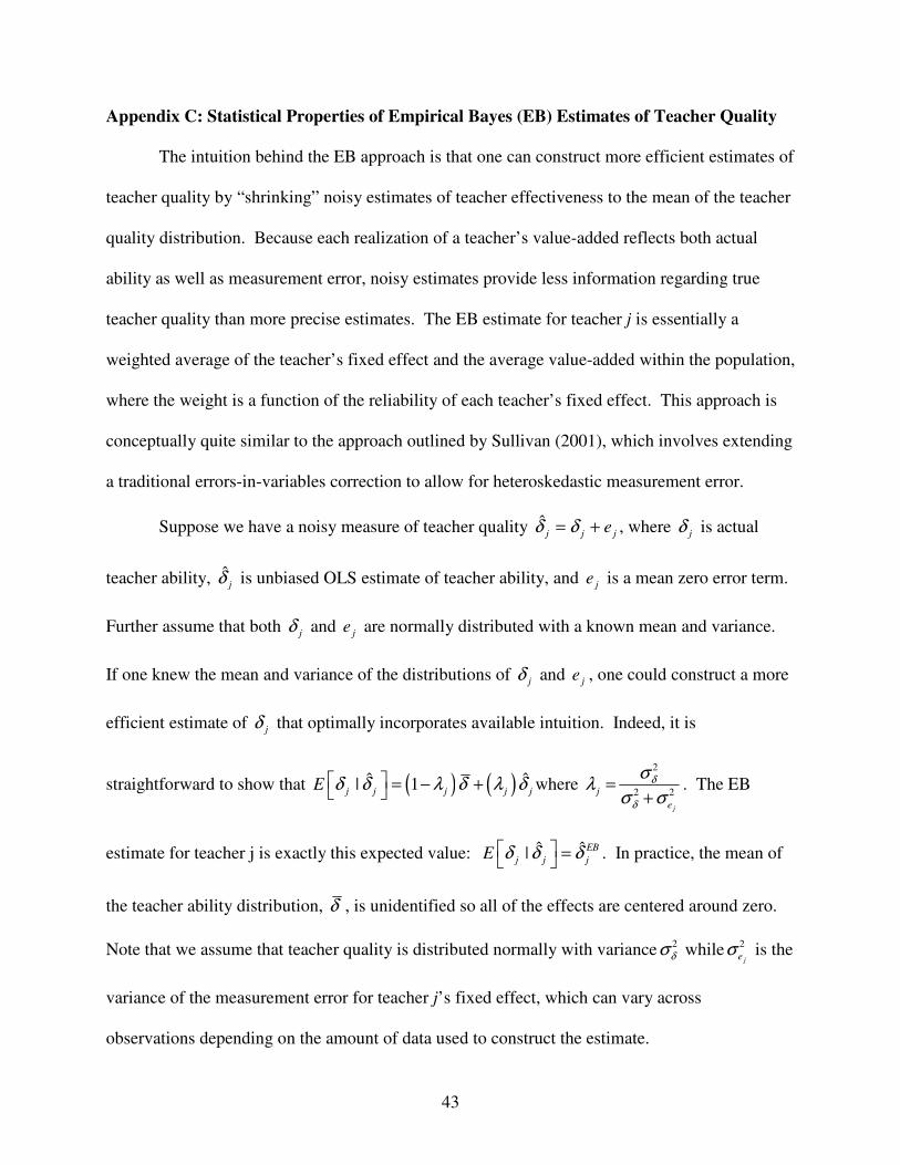
43

Appendix C: Statistical Properties of Empirical Bayes (EB) Estimates of Teacher Quality

The intuition behind the EB approach is that one can construct more efficient estimates of

teacher quality by “shrinking” noisy estimates of teacher effectiveness to the mean of the teacher

quality distribution. Because each realization of a teacher’s value-added reflects both actual

ability as well as measurement error, noisy estimates provide less information regarding true

teacher quality than more precise estimates. The EB estimate for teacher j is essentially a

weighted average of the teacher’s fixed effect and the average value-added within the population,

where the weight is a function of the reliability of each teacher’s fixed effect. This approach is

conceptually quite similar to the approach outlined by Sullivan (2001), which involves extending

a traditional errors-in-variables correction to allow for heteroskedastic measurement error.

Suppose we have a noisy measure of teacher quality ˆj j jeδ δ= + , where jδ is actual

teacher ability, ˆjδ is unbiased OLS estimate of teacher ability, and je is a mean zero error term.

Further assume that both jδ and je are normally distributed with a known mean and variance.

If one knew the mean and variance of the distributions of jδ and je , one could construct a more

efficient estimate of jδ that optimally incorporates available intuition. Indeed, it is

straightforward to show that ( ) ( )ˆ ˆ| 1j j j j jE δ δ λ δ λ δ� = − + � where 2

2 2j

je

δ

δ

σλσ σ

=+

. The EB

estimate for teacher j is exactly this expected value: ˆ ˆ| EBj j jE δ δ δ� = � . In practice, the mean of

the teacher ability distribution, δ , is unidentified so all of the effects are centered around zero.

Note that we assume that teacher quality is distributed normally with variance 2δσ while 2

jeσ is the

variance of the measurement error for teacher j’s fixed effect, which can vary across

observations depending on the amount of data used to construct the estimate.

44

Of course, the mean of the teacher quality distribution and the variance of the error term

are not generally known and must be estimated. One can construct an empirical analog to the

expectation above using the method proposed by Morris (1983). This essentially involves using

the estimated mean and variance to calculate the appropriate shrinkage factor, jλ , and

incorporating an appropriate degrees of freedom adjustment.39 We will refer to this estimate as

ˆEBjδ . The resulting properties of this EB estimate are essentially the same as if these parameters

were known, so for simplicity we will act as if the parameters were known for the remainder of

the discussion.

One can easily show that using the EB estimates as an explanatory variable in a

regression context will yield point estimates that are unaffected by the attenuation bias that

would exist if one used simple OLS estimates. Define the error of the EB estimate as jv , so

that ˆEBj j jvδ δ= + . Because the EB procedure takes advantage of all available information to

construct the estimated teacher effect — indeed it is the empirical analog to the conditional

expectation of jδ — the shrinkage estimator is uncorrelated with the error term: ˆcov( , ) 0EBv δ = .

In fact, the shrinkage estimate can also be thought of as the predicted value from a regression of

the actual teacher quality on the noisy measure. By construction, this prediction is orthogonal to

the residual jv .

Too see that the EB estimate of teacher quality will yield unbiased estimates when used

as an explanatory variable in a regression context, consider the following simple regression

equation:

39 The degrees of freedom adjustment takes into account that the mean that we are shrinking toward is estimated—not known.

45

(C1)

0 1

0 1 1ˆ

j j j

EBj j j

y u

v u

β β δ

β β δ β

= + +

= + + + .

Because, ˆEBjδ is orthogonal to the composite error term, 1 j jv uβ + , we know the resulting

estimate of 1β will be unbiased.

Now suppose that it is known that the distribution of value added varies across a set of K

different groups. For example, the distribution of actual teacher quality may vary by gender or

experience. In this case, the conditional expectation of jδ is

( ) ( )ˆ ˆ| , 1j j j k j jE group kδ δ λ δ λ δ= = − + , where kδ is the mean of teacher quality of teachers in

group k. Additionally, jλ must be constructed using the variance of jδ around the group-

specific mean. Morris’ (1983) method of constructing EB estimates readily generalizes to this

situation, though in practice it may be necessary to impose substantial structure on the

conditional mean.40 The advantage of allowing the mean of the teacher quality measure to vary

with covariates is that one can generate more precise estimates of teacher quality. Furthermore,

the error of the EB estimate will be orthogonal to every piece of information (e.g. gender) used

to construct it. This guarantees regression coefficient estimates that are unbiased by

measurement error in a context that includes covariates besides the EB measure itself.

40 For example, one may need to assume that the conditional mean of teacher ability is a quadratic function of experience to conserve degrees of freedom.

46

Appendix D: OLS Estimates of Parent Requests

Tables VI and VII explore the heterogeneity in parent preferences across family

demographics. Since we do not have student-level request information, we calculate the average

demographic characteristics of all students in each school-grade-year (e.g., the fraction of

students who are eligible for free lunch). We then categorize school-grade-year observations on

the basis of these aggregate demographic measures. To focus on educational outputs, we regress

our normalized parent request variable on the principal’s assessment of a teacher’s ability to

promote student satisfaction and to promote student achievement (including fixed effects for

school-grade-year, but no other covariates). Table D1 shows the OLS estimates for several

different subgroups. Column 2, for example, presents estimates for school-grade-year

observations in which fewer than 50 percent of students were eligible for free lunch. In this

group, a teacher’s student satisfaction rating is strongly related to the number of requests that he

or she receives. The coefficient on a teacher’s achievement rating is substantially smaller and

not significantly different than zero. In contrast, in classes where at least 50 percent of students

were eligible for free lunch, a teacher’s student satisfaction rating has no effect on his or her

requests, but a teacher’s achievement rating has a strong, positive effect on parent requests. A

similar but even stronger pattern is apparent if one compares school-grade-year observations

where fewer than (or at least) 20 percent of students are minority. The estimates in columns 6-7

that show the results by prior student achievement level suggest that this finding may be partially

related to student achievement. 41 Table VI presents estimates from a specification that, as

41 We use test scores from the prior year to determine the percent of students scoring in the top half of the district distribution in a school-grade-year. Because we do not have student test scores for the 2003-04 school year, we use test scores for the 2002-03 school year to calculate the prior ability of the cohorts entering in 2004-05. Unfortunately, we do not have first grade test scores for 2002-03. For this reason, we must exclude second grade classes in both 2003-04 and 2004-05 and third grade classes in 2004-05 from the analyses shown in columns 5-6 in Tables V-A and V-B as well as columns 8-10 in Tables VII-A and VII-B. This is one reason that the reduced precision of these results.

47

above, includes the student satisfaction measure, but replaces the principal-reported teacher

achievement measure with the teacher value-added measure. The results are qualitatively the

same.

48

TABLE D-1 OLS ESTIMATES OF HETEROGENEITY IN PARENTAL PREFERENCES BY FAMILY DEMOGRAPHICS

Independent Variable Full Sample

Less than 50% of students eligible for

free or reduced price

lunch

At least 50% of students eligible for

free or reduced price

lunch

Less than 20% of students are

minority

At least 20% of students are

minority

Less than 50% of students with above

average achievement

scores

At least 50% of students with above

average achievement

scores

(1) (2) (3) (4) (5) (6) (7) Principal’s evaluation of the teacher’s ability to promote student satisfaction (composite measure from factor analysis)

0.045* (0.009)

0.057* (0.012)

0.012 (0.009)

0.075* (0.013)

0.017* (0.007)

0.020† (0.012)

0.055* (0.015)

Principal’s evaluation of the teacher’s ability to raise student achievement (composite measure from factor analysis)

0.022* (0.011)

0.019 (0.015)

0.026* (0.010)

0.019 (0.016)

0.034* (0.010)

0.046* (0.015)

0.022 (0.017)

Number of observations 251 150 101 113 138 56 122 Fraction of parents requesting any teacher 0.284 0.352 0.190 0.376 0.207 0.213 0.326

Average fraction of parents requesting the an individual teacher 0.092 0.114 0.061 0.126 0.063 0.070 0.111

Notes: The unit of observation is teacher-grade-school-year. The sample includes only grades 2-6. For columns 5-6, the sample omits some observations for which prior student achievement measures are not available. The dependent variable is the number of parent requests, normalized by subtracting off the average number of requests in the grade-school-year and then dividing by the student enrollment in the grade-school-year. Demographics are measured at the school-grade-year level. All models include fixed effects for school-grade-year. Standard errors clustered by teacher are shown in parentheses. * = significant at 5 percent level. † = significant at 10 percent level.

49

TABLE D-2 OLS ESTIMATES OF HETEROGENEITY IN PARENTAL PREFERENCES BY FAMILY DEMOGRAPHICS

Independent Variable Full Sample

Less than 50% of students eligible for

free or reduced price

lunch

At least 50% of students eligible for

free or reduced price

lunch

Less than 20% of students are

minority

At least 20% of students are

minority

Less than 50% of students with above

average achievement

scores

At least 50% of students with above

average achievement

scores

(1) (2) (3) (4) (5) (6) (7) Principal’s evaluation of the teacher’s ability to promote student satisfaction (composite measure from factor analysis)

0.054* (0.007)

0.067* (0.009)

0.024* (0.009)

0.083* (0.011)

0.031* (0.006)

0.036* (0.012)

0.063* (0.012)

Teacher value-added 0.025

(0.036) -0.075 (0.047)

0.079* (0.040)

-0.042 (0.065)

0.061 (0.039)

-0.003 (0.068)

-0.022 (0.072)

Number of observations 150 101 113 138 56 122 Fraction of parents requesting any teacher 0.284 0.352 0.190 0.376 0.207 0.213 0.326

Average fraction of parents requesting a particular teacher 0.092 0.114 0.061 0.126 0.063 0.070 0.111

Notes: The unit of observation is teacher-grade-school-year. The sample includes only grades 2-6. For columns 5-6, the sample omits some observations for which prior student achievement measures are not available. The dependent variable is the number of parent requests, normalized by subtracting off the average number of requests in the grade-school-year and then dividing by the student enrollment in the grade-school-year. Demographics are measured at the school-grade-year level. All models include fixed effects for school-grade-year. Standard errors clustered by teacher are shown in parentheses. * = significant at 5 percent level. † = significant at 10 percent level.

50

FIGURE I

0.0

5.1

.15

Fra

ctio

n

0 10 20 30 40

Number of Requests

Distribution of Parent Requests

FIGURE II

0.0

2.0

4.0

6.0

8Fr

actio

n

0 10 20 30

Number of Requests

Difference between most and least requested class in the grade

51

FIGURE III

05

1015

20

Ran

k of

par

ent r

eque

sts

in 2

004

0 5 10 15 20

Rank of parent requests in 2003

Peristence of Parental Requests over Time

52

FIGURE IV DISTRIBUTION OF PRINCIPAL RATINGS WITHIN SCHOOL

0.1

.2.3

.4.5

Frac

tion

-6 -5 -4 -3 -2 -1 0 1 2 3 4 5 6Deviation from Median Rating

Distribution of Principal Reading Ratings0

.1.2

.3.4

.5Fr

actio

n

-6 -5 -4 -3 -2 -1 0 1 2 3 4 5 6Deviation from Median Rating

Distribution of Principal Math Ratings

0.1

.2.3

.4.5

Frac

tion

-6 -5 -4 -3 -2 -1 0 1 2 3 4 5 6Deviation from Median Rating

Distribution of Principal Reading Ratings

53

TABLE I SUMMARY STATISTICS

Overall Range within choice set (i.e., school-grade-year)

Teacher Characteristic Mean Standard deviation

Mean of range

25th percentile of

range

75th percentile of

range Male 0.14 0.34 0.36 0 1 Age 43.69 12.58 19.24 10 29 First year teacher 0.09 0.28 0.29 0 1 2-5 years of experience 0.16 0.36 0.47 0 1 6-10 years of experience 0.23 0.42 0.56 0 1 11-20 years of experience 0.21 0.41 0.52 0 1 21+ years experience 0.31 0.46 0.58 0 1 First year in the school (with >1 year of experience) 0.07 0.26 0.28 0 1

BA Degree at in state (but not local) college 0.14 0.35 0.40 0 1 BA Degree at out of state college 0.04 0.19 0.16 0 0 MA Degree 0.15 0.36 0.42 0 1 Any additional endorsements 0.22 0.41 0.48 0 1 Enrollment in grade-school-year 79.18 15.61 0 0 0 Mixed grade classroom 0.10 0.31 0.12 0 0 Two teachers in the classroom 0.03 0.18 0.09 0 0 Dual language classroom 0.02 0.13 0.05 0 0 Number of positive requests 6.88 6.91 10.96 6 15 Number of negative requests 0.35 1.10 0.98 0 2 Teacher Value-Added (EB estimate of math-reading composite) 0.00 0.18 0.20 0.07 0.29

Student satisfaction factor 0.05 1.00 1.29 0.05 2.14 Student achievement factor 0.09 0.88 1.25 0.39 2.16 Teacher collegiality factor 0.06 0.91 1.27 0.38 1.85 Overall teacher effectiveness 8.09 1.22 1.48 0.5 2 Dedication and work ethic 8.50 1.50 1.75 0 3 Organization 7.97 1.55 1.99 1 3 Classroom management 8.02 1.63 1.67 0 3 Raising student math achievement 7.84 1.30 1.44 0 2 Raising student reading achievement 7.78 1.37 1.56 0 3 Role model for students 8.40 1.19 1.50 1 2 Student satisfaction with teacher 8.35 1.06 1.25 0 2 Parent satisfaction with teacher 8.28 1.16 1.50 1 2 Positive relationship with colleagues 7.93 1.64 1.72 0 2 Positive relationship with administrators 8.43 1.55 1.55 0 2 Notes: Nearly all teachers in the district are Caucasian, so race indicators are omitted.

54

TABLE II WHICH PARENTS MAKE REQUESTS?

Dependent Variable = Fraction of Parents Making Requests (1) (2) (3) (4) (5) (6)

% male -0.44 (0.42)

-0.29 (0.25)

-0.21 (0.28)

% eligible for free lunch -0.52* (0.13)

-0.32 (0.28)

-0.54* (0.14)

% minority -0.72* (0.17)

-0.32 (0.32)

% receiving special education services

-0.34 (0.55)

0.29 (0.50)

0.49 (0.42)

Number of observations 80 80 80 80 80 80 R-squared 0.04 0.37 0.36 0.02 0.40 0.39 Notes: The unit of observation is a school-grade-year (n=80). Each column represents a separate OLS regression. All models also include grade fixed effects. Standard errors clustered at the school-year level are shown in parentheses. * = significant at 5 percent level. † = significant at 10 percent level.

55

TABLE III FACTOR LOADINGS DERIVED FROM PRINCIPAL RATING ITEMS

Item Factor 1 - Student

Satisfaction

Factor 2 – Achievement

Factor 3 - Collegiality

Dedication and work ethic -0.132 0.664 0.165 Organization 0.004 0.830 0.013 Classroom management 0.184 0.827 -0.175 Raising student math achievement -0.005 0.775 0.028 Raising student reading achievement -0.018 0.783 0.056 Role model for students 0.446 0.236 0.290 Student satisfaction with teacher 0.967 0.008 0.046 Positive relationship with colleagues 0.037 -0.034 0.872 Positive relationship with administrators 0.055 -0.026 0.844

Notes: Factors derived from ML factor analysis with a Promax rotation that excludes the parent satisfaction item. All individual survey items are normalized.

56

TABLE IV BASELINE ESTIMATES OF PARENT REQUESTS

OLS Estimates Structural Estimates

(1) (2) (3) (4) (5) (6) (7)

2-5 years of experience 0.077* (0.026) 0.075*

(0.031)

1.105* (0.493) [0.098]

6-10 years of experience 0.054* (0.021) 0.034

(0.032)

0.876† (0.494) [0.073]

11-20 years of experience 0.085* (0.024) 0.061†

(0.036)

1.038† (0.535) [0.089]

21+ years experience 0.017 (0.024) 0.043

(0.031)

0.821 (0.515) [0.066]

First year in the school (with >1 year of experience)

-0.048* (0.019) -0.036

(0.027)

-0.424 (0.398) [-0.029]

Male 0.012 (0.026) 0.025

(0.020)

0.237 (0.184) [0.018]

BA Degree at in state (but not local) college

-0.006 (0.021) -0.003

(0.017)

0.028 (0.251) [0.002]

BA Degree at out of state college

-0.020 (0.027) -0.012

(0.027)

-0.104 (0.361) [-0.008]

MA Degree 0.009 (0.021) 0.026

(0.021)

0.336† (0.204) [0.026]

Any additional endorsements -0.008 (0.022) -0.018

(0.017)

-0.168 (0.160) [-0.012]

Mixed grade classroom -0.067* (0.026) -0.028*

(0.020)

-0.483 (0.326) [-0.033]

Two teachers in the classroom 0.070* (0.031) 0.042*

(0.021)

0.487 (0.803) [0.040]

Dual language classroom 0.024 (0.033) 0.007

(0.027)

0.849 (2.884) [0.077]

Teacher value-added in reading and math 0.062

(0.050) -0.025 (0.041)

-0.026 (0.047)

-0.057 (0.572) [-0.004]

Principal’s evaluation of the teacher’s ability to raise student 0.047*

(0.010) 0.032* (0.011)

0.024* (0.010)

0.264* (0.109)

57

achievement (composite) [0.020] Principal’s evaluation of the teacher’s ability to promote student satisfaction (composite)

0.055* (0.007)

0.057* (0.009)

0.058* (0.009)

0.582* (0.082) [0.043]

Principal’s evaluation of the teacher’s collegiality (composite)

-0.029* (0.011)

-0.026* (0.010)

-0.191† (0.108) [-0.014]

Number of observations 251 251 251 251 251 251 331 Chi-square (p-value) of test of joint significance of grade fixed effects in the cost function

6.00 (0.20)

Chi-square (p-value) of test of joint significance of school fixed effects in the cost function

60.91 (0.00)

Notes: Sample includes grades 2-6. For columns 1-6, the unit of observation is the teacher-grade-school-year (n=251). The dependent variable is the number of parent requests, normalized by subtracting off the average number of requests in the grade-school-year and then dividing by the student enrollment in the grade-school-year. All models include fixed effects for school-grade-year. The fraction of parents requesting any teacher in the sample is 0.283 and the average fraction of parents requesting any individual teacher is 0.095. Standard errors are clustered by teacher. Column 7 presents estimates of the preference parameters from the structural model. The parentheses contain standard errors that are estimated via a bootstrap and the square brackets contain the average marginal effect of the variable on each teacher’s share, which is roughly comparable to the OLS point estimates. * = significant at 5 percent level. † = significant at 10 percent level.

58

TABLE V STRUCTURAL ESTIMATES OF DIFFERENTIAL EFFECTS OF PARENT PREFERENCES BY FAMILY DEMOGRAPHICS

All Students

Eligible for free lunch

Not eligible for free lunch

Diff. Minority Non-Minority Diff.

Bottom Half of

Test Scores

Top Half of Test Scores

Diff.

(1) (2) (3) (4) (5) (6) (7) (8) (9) (10) Principal Student

Satisfaction Factor

Structural Coefficient

0.515* (0.064)

-0.061 (0.283)

0.837* (0.195)

-0.898* (0.444)

-0.437 (0.439)

0.708* (0.132)

-1.145* (0.530)

-0.156 (0.248)

1.152* (0.259)

-1.308* (0.432)

Marginal Effect [Relative Effect]

0.039 [0.351]

-0.004 [-0.042]

0.068 [0.571] -0.072 -0.029

[-0.295] 0.056

[0.484] -0.085 -0.013 [-0.104]

0.085 [0.759] -0.098

Principal

Achievement Factor

Structural Coefficient

0.226* (0.093)

0.740* (0.271)

-0.038 (0.237)

0.778† (0.466)

1.172* (0.430)

0.056 (0.148)

1.116* (0.522)

0.695† (0.351)

-0.058 (0.300)

0.743 (0.561)

Marginal Effect [Relative Effect]

0.017 [0.154]

0.052 [0.505]

-0.003 [-0.026] 0.055 0.079

[0.796] 0.004

[0.038] 0.075 0.057 [0.466]

-0.004 [-0.031] 0.061

Notes: Sample includes only grades 2-6 (n=331). Demographics are measured at the school-grade-year level. * = significant at 5 percent level. † = significant at 10 percent level.

59

TABLE VI STRUCTURAL ESTIMATES OF DIFFERENTIAL EFFECTS OF PARENT PREFERENCES BY FAMILY DEMOGRAPHICS

All Students

Eligible for free lunch

Not eligible for free lunch

Diff. Minority Non-Minority Diff.

Bottom Half of

Test Scores

Top Half of Test Scores

Diff.

(1) (2) (3) (4) (5) (6) (7) (8) (9) (10) Principal Student

Satisfaction Factor

Structural Coefficient

0.599* (0.055)

0.436* (0.211)

0.706* (0.121)

-0.270 (0.307)

0.416 (0.339)

0.648* (0.082)

-0.232 (0.414)

0.195 (0.240)

1.054* (0.274)

-0.859† (0.465)

Marginal Effect [Relative Effect]

0.045 [0.408]

0.030 [0.297]

0.059 [0.481] -0.029 0.026

[0.282] 0.053

[0.443] -0.027 0.017 [0.131]

0.079 [0.694] -0.062

Teacher

Composite Value-Added Measure

Structural Coefficient

0.433 (0.383)

2.999† (1.589)

-1.864 (1.465)

4.863† (2.850)

6.034† (3.170)

-1.245 (0.886)

7.279* (3.410)

0.113 (1.589)

-0.358 (2.237)

0.471 (3.618)

Marginal Effect [Relative Effect]

0.033 [0.295]

0.208 [2.046]

-0.156 [-1.269] 0.364 0.385

[4.095] -0.101

[-0.850] 0.486 0.010 [0.076]

-0.027 [-0.235] 0.037

Notes: Sample includes only grades 2-6 (n=331). Demographics are measured at the school-grade-year level. * = significant at 5 percent level. † = significant at 10 percent level.

60

TABLE VII DOES THE LEVEL AND VARIATION IN TEACHER QUALITY MEASURES DIFFER ACROSS SCHOOLS?

Dependent Variables

Level of Teacher Characteristics Range of Teacher Characteristics

Within Each Choice Set (i.e., school*grade*year)

Independent Variables Value-Added

Average Math and Reading Rating

Average organization

and management

rating

Student Satisfaction

Rating

Value-Added

Average Math and Reading Rating

Average organization

and management

rating

Student Satisfaction

Rating

% eligible for free-lunch 0.026

(0.027) 1.00

(0.88) 1.47

(1.15) 1.07

(0.74) 0.03

(0.06) -2.51† (1.15)

-3.13* (0.92)

-1.30* (0.51)

R-squared 0.006 0.022 0.035 0.035 0.002 0.114 0.167 0.063 F-stat (p-value) of joint significance of the regression that includes school fixed effects but no other covariates

0.11 (1.00)

4.66 (0.00)

5.45 (0.00)

3.29 (0.00)

1.47 (0.17)

4.35 (0.00)

2.16 (0.03)

0.99 (0.46)

Number of observations 198 202 202 202 80 79 79 79 Notes: The unit of observation for columns 1-4 is a teacher-year. The unit of observation for columns 5-8 is a school-grade-year. The percent eligible for free-lunch is the average for a grade-school-year. Estimates are based on OLS regressions with standard errors clustered by school. We do not include our baseline value-added measures because they include school fixed effects. Instead we use a specification that does not include school fixed effects but does include student fixed effects to address concerns regarding unobserved heterogeneity across schools. * = significant at 5 percent level. † = significant at 10 percent level.

61

Table VIII ARE REQUESTING PARENTS SIMILAR TO NON-REQUESTING PARENTS?

School 116 School 122

Full district sample All Students Students who

made requests

All Students Students who made requests

% eligible for free lunch 0.48 0.66 0.38 0.29 0.09 % minority 0.27 0.44 0.24 0.15 0.06 % Hispanic 0.21 0.36 0.15 0.06 0.01 % other minority 0.06 0.08 0.09 0.09 0.05 % limited English proficient 0.21 0.37 0.20 0.10 0.02

% special education 0.12 0.13 0.06 0.12 0.11 Number of observations 5783 391 68 461 141 Percent of parents who made a request 0.17 0.31

Notes: Sample includes all students from school 116 in 2003-04 and school 122 in 2004-05.

62

TABLE IX SENSITIVITY ANALYSES

Student Satisfaction Factor

Structural Coefficient [Marginal Effect]

Achievement Factor Structural Coefficient

[Marginal Effect]

Eligible for Free Lunch

Not eligible for free lunch

Eligible for Free Lunch

Not eligible for free lunch

Baseline Cost function includes grade and school fixed effects. Preference function includes only principal-based student satisfaction and student achievement factors.

-0.061 [-0.004]

0.837* [0.068]

0.740* [0.052]

-0.038 [-0.003]

Alternative Specifications of the Cost Function

Include only grade fixed effects -0.228 [-0.010]

0.692* [0.071]

1.275 [0.058]

0.017 [0.002]

Include school-grade-year fixed effects -0.111 [-0.008]

0.979* [0.077]

0.624* [0.045]

-0.001 [0.000]

Alternative Specification of the Preference Parameters

Includes principal-based teacher collegiality factor.

-0.109 [-0.008]

0.980* [0.080]

0.641† [0.045]

0.112 [0.009]

Includes measures of experience and experience squared along with dummy variables for male and MA degree as well as principal-based collegiality factor.

-0.155 [-0.010]

0.915* [0.075]

0.527 [0.034]

0.141 [0.012]

Alternative Measure of Parent Requests

Include negative as well as positive requests -0.108 [-0.008]

0.929* [0.077]

0.740* [0.055]

-0.057 [-0.005]

Alternative Principal Measures Using principal-reported measures of a teacher’s ability to promote student satisfaction and raise student achievement that are by construction orthogonal to the principal’s report of parent satisfaction

0.064 [0.005]

0.828† [0.071]

0.786 [0.056]

-0.125 [-0.011]

Alternative Assumption Regarding Value of Not Making a Request

Expected teacher quality if no request is made takes into account that the probability of being assigned to a classroom depends on the popularity of the teacher

-0.090 [-0.006]

0.722* [0.056]

0.929* [0.060]

-0.078 [-0.006]

Notes: Sample includes only grades 2-6 (n=331). Demographics are measured at the school-grade-year level. * = significant at 5 percent level. † = significant at 10 percent level.