What Determines the Number of Firms?

Cost Structure and Producer Concentrationin Homogeneous Product Industries

Marvin B. Lieberman

Anderson Graduate School of Management

UCLA

Los Angeles, CA 90024-1481

Tel.: (310) 206-7665

Fax: (310) 206-3337

E-Mail: marvin.lieberman@anderson.ucla.edu

July 30, 1999

I thank John Sutton, Anita McGahan and seminar participants at the the Harvard Business Schoolfor helpful insights. Comments on an early version of this paper were provided by Mark Roberts,Pankaj Ghemawat, and seminar participants at Berkeley, UCLA, USC and the United StatesDepartment of Justice. I am indebted to Curtis Eaton, who collaborated in the initial phase of thisstudy.

1

ABSTRACT

This study considers how cost structure affects producer concentration in

homogeneous product industries. Tests are performed on a sample of 31 chemical

products. By applying the “Dixit” cost function to engineering data, sunk costs are

parameterized into two elements: (a) the industry “entry fee,” and (b) the ratio of sunk to

variable costs. These aspects of sunk cost are shown to have distinct but opposite effects:

the number of producers falls with the entry fee but rises with the sunk cost ratio. Thus,

sunk costs may contribute to either an increase or a decrease in industry concentration,

depending on how the cost components are distributed. These findings help to resolve

ambiguities in prior work on sunk costs.

2

1. Introduction

What determines the number of competitors in a homogeneous product industry?

Recent theoretical work highlights the potential influence of cost structure, particularly the

presence of sunk costs. A standard result is that the number of firms falls with the

investment required for market entry. In addition, if firms make large, irreversible

investments in production capacity, incumbent producers may be able to deter new entry

strategically. Yet sunk costs also create a gap between an industry’s entry- and exit-

inducing prices, which can lead to an overabundance of producers and negative economic

profits. Economic theory thus gives conflicting predictions: higher sunk costs seem likely

to reduce, but may possibly increase, the number of competing firms.

This paper investigates how sunk costs affect producer concentration in

homogeneous product industries where capacity commitments are important. Tests are

performed on a sample of 31 chemical products for which engineering cost estimates were

obtained. These estimates are mapped into the “Dixit” cost function, commonly used in

theoretical work. The resulting measures allow the effects of cost structure to be

evaluated in a conventional regression analysis, unlike prior studies that have inferred the

role of cost structure from information on entry and changes in demand.

Using the engineering data, sunk costs are separated into two components. The

first corresponds to the industry’s “entry fee.” The second reflects the extent to which

total costs are sunk. The regression results show that these two features of sunk cost

have distinct but opposite effects: the number of producers falls with the entry fee and

rises with the proportion of costs that are sunk. Thus, sunk costs may contribute to either

an increase or a decrease in industry concentration, depending on how the cost

components are distributed. These empirical findings are new and help to resolve the

ambiguity raised by theoretical work.

3

The primary data sample for this study is for producers in the United States, with

supplementary information on Western Europe and Japan. In addition to the producer

count and engineering cost data, historical information was collected on the annual output

of each product, which provides an indicator of demand. The regression results imply that

in all three geographic regions, the number of producers was largely determined by cost

structure and market size.

The paper is organized as follows. The next section surveys the literature on

potential determinants of producer concentration. Section 3 describes the sample of

chemical products, the parameterization of cost structure, and the specific measures used

in the study. Section 4 presents the regression estimates. A concluding section

summarizes the findings and relates them to prior work.

2. Cost Structure and Industry Concentration

Views on the influence of cost structure on market concentration have evolved

since the 1950s. Early empirical studies focused on the effects of plant-level economies of

scale. These studies typically regressed producer concentration on various proxies for

scale economies and found a high correlation, particularly for industries with minimal

advertising and R&D expenditures (c.f., Curry and George, 1983). Other work revealed

that industry concentration levels were similar across countries (but decreasing, generally,

with the size of the national market) which implied a strong underlying force of

technological determinism (Bain, 1956; Pashigian, 1969; Pryor, 1972; Scherer, 1973;

George and Ward, 1975).

More recently, economists have aimed at more precise assessments by drawing a

distinction between costs that are fixed but recoverable, and those that are irretrievably

sunk.1 For given level of demand, the equilibrium number of producers generally declines

1 Fixed costs may take various forms; e.g., output-invariant fees or input charges, or initial setup costs.Typically, some proportion of setup costs are not only fixed but also unrecoverable, i.e., sunk.

4

with the magnitude of fixed costs.2 Sunk costs, however, lead to more complicated

dynamic outcomes, where a diversity of theoretical results have been demonstrated.

One line of theoretical research on sunk costs (e.g., Dixit, 1980; Eaton and Ware,

1987) demonstrates how early entrants may be able to preempt a growing market. These

models assume a cost structure similar to the chemical industries evaluated in this study:

firms undertake investments to enter the industry, and then to expand capacity. Sunk

costs provide a means for producers to commit to higher future output. The models show

that under some cost and demand conditions, early entrants can invest strategically to

deter subsequent entry.

Other research (e.g., Dixit, 1989; Bresnahan and Reiss, 1993) shows that in the

presence of uncertainty, sunk costs lead to hysteresis---a gap between the prices that

induce entry and exit---which expands the set of equilibrium market structures. If cost or

demand are uncertain, firms may rationally enter and persist, even though they are unable,

ex post, to earn economic profits. Such results are extensions of Marshall’s classic model

in which firms enter an industry when demand covers fixed plus variable costs and exit

only when price falls below variable cost. MacLeod (1987) shows that as the proportion

of costs that are sunk increases, it is possible to have a larger number of firms forming an

equilibrium market structure. This is the opposite of the predictions of the sunk cost

deterrence models.

Sutton (1991) draws an important distinction between exogenous and endogenous

sunk costs. He considers exogenous sunk costs to be the technologically determined

setup costs required for industry entry.3 Sutton shows that in homogeneous product

2 In models where profits fall with the number of competitors, entry occurs up to the point where anadditional entrant is unable to cover fixed costs. With higher fixed costs, this profit constraint leads tofewer firms in the industry.3 In his analysis of homogeneous product industries, Sutton considers only the initial “entry fee,” ignoringthe additional sunk costs relating to expansion of capacity. Both sets of sunk costs are considered in thepresent study.4 For example, R&D, advertising, and other reputational capital are not normally recorded as assets on thefirm’s books. Measures of tangible capital that are standard items on the balance sheet may be biased byaccelerated depreciation accounting.

5

industries, where sunk costs are mostly exogenous, bounds on producer concentration are

defined by the size of the market relative to the setup cost of entry. Increases in market

size and reductions in the entry fee lead to (potentially) larger numbers of firms.

Endogenous sunk costs, such as advertising and R&D, serve to enhance the

demand for the firm’s product. Sutton argues that normal processes of competition

induce firms to escalate these investments, thereby reducing the number of firms. This

may explain why advertising and R&D-intensive industries are often much more

concentrated than would be expected on the basis of manufacturing economies of scale.

Sutton’s work suggests that the effects of sunk costs in promoting concentration may be

greatest in differentiated product industries where the potential rewards to advertising and

other intangible assets are unbounded. Sutton presents empirical evidence on the food and

drink sector to support these predictions on the effects of exogenous and endogenous

sunk costs.

Other empirical findings on the connection between sunk costs and concentration

have been more equivocal. This may stem from the theoretical ambiguities described

above, or to the difficulty of accurately identifying cost structures. Kessides (1990) found

that industries were less concentrated when the sunkenness of capital was limited by rapid

depreciation or by the availability of leases or resale markets. This finding is consistent

with market preemption based on sunk costs. Gilbert (1986), however, surveyed

accounting data for a range of industries and concluded that in most cases the degree of

capital intensity is too low for deterrence to be effective. Similarly, Lieberman (1987)

found little evidence that incumbents in chemical product markets preempted by building

capacity ahead of demand.

In other recent studies that assess the relation between cost structure and

concentration (e.g., Reiss and Spiller, 1989; Bresnahan and Reiss, 1990, 1991; Berry,

1992), costs are inferred by observing entry and exit in response to changes in demand.

This approach has the advantage that it avoids the use of accounting data, which may be

biased.4 These studies confirm that cost structure and demand factors can jointly explain

6

much of the systematic variation in industry concentration levels. However, the “entry

thresholds” demonstrated in these studies fail to suggest widespread preemption or entry

deterrence through the use of sunk costs.

Various empirical work points to the prevalence of hysteresis effects. Bresnahan

and Reiss (1993) found evidence of hysteresis in the entry and exit behavior of dentists in

small rural markets, which they attributed to sunk costs. Ghemawat and Caves (1986)

found profits to be negatively correlated with capital intensity, a result consistent with

hysteresis but not with predictions of the sunk cost commitment models. Numerous

studies in the international trade literature (e.g., Baldwin, 1988) show persistence in trade

flows which can be explained by hysteresis in firms’ underlying infrastructure investments.

Other studies have focused on changes in concentration over the life cycle of an

industry. A common finding is that the number of firms tends to increase as demand

grows over time, although at some point a “shakeout” of producers commonly occurs

(Klepper and Graddy, 1990). Yet even when concentration remains stable, firm turnover

(entry counterbalanced by exit) is often substantial. High turnover rates have been

observed for most manufacturing industries, including those in the chemical products

sector (Dunne, Roberts and Samuelson, 1988, 1989).

3. Data and Measures

The tests in this study were performed by regressing producer counts for the

chemical products on a set of cost structure and demand-side measures. The resulting

coefficients can be regarded as reduced form estimates of the determinants of producer

concentration. Given that concentration and output are likely to be endogenous (in

particular, the price and volume of output may depend upon the number of producers), the

regressions were estimated using instrumental variables. The data sample and measures

used in the analysis are described below.

7

Chemical Products Sample

The data sample includes 31 commodity industrial chemicals for which suitable

data on cost structure, plant capacity and total industry output could be obtained for the

1970s and 1980s.5 Table 1 lists these chemicals and corresponding counts of producers in

the US, Western Europe and Japan. The 31 products are homogeneous and

undifferentiated among producers; and all but two (hydrogen peroxide and nitric acid) are

petrochemicals.

For most products in the sample, total output grew rapidly from the 1950s through

the early 1970s, which was the major growth phase of the U.S. petrochemical sector. The

engineering cost estimates used in this study pertain to new plants built in 1977.

Regression analyses were performed for the number of producers in that year and also in

the late 1980s, recognizing that some time may have been required for process technology

that was state-of-the-art in 1977 to become widely adopted.

By the 1970s the chemical product industries in the sample could reasonably be

characterized as mature. Demand growth and technical progress had slowed considerably

from the pace of the prior two decades. Moreover, production technology was widely

available through licensing, and it had become common for new plants to be designed and

built by independent engineering contractors (Freeman, 1968; Spitz, 1988; Stobaugh,

1988; Arora and Gambardella, 1998). Thus, restricted access to technology was not a

significant barrier to entry, and firms’ internal R&D activities had become relatively

unimportant.

For purposes of this study, the 31 chemical products in the sample are each

considered to represent a separate industry. Furthermore, the three geographic regions

(United States, Western Europe and Japan) are assumed to be independent. These

5 The sample includes all industrial chemicals that met the following criteria: (1) data on plant capacityand number of producers are listed in the 1977 SRI Directory of Chemical Producers, United States; (2)industry output data are publicly available; (3) plants cannot easily be converted to make other products;(4) engineering cost estimates are listed in the 1977 SRI Processes Economics Program Yearbook; and (5)the Yearbook shows only a single manufacturing process for the chemical (or if there are multipleprocesses, their cost structures are very similar).

8

assumptions are reasonable approximations to reality. The chemical plants represented in

the study are each dedicated to the manufacture of a specific product; the sample excludes

chemicals whose production processes yield significant joint products, and those where

capacity is convertible to other products.6 While industrial chemicals are shipped

internationally in large quantities, the volume of trans-oceanic trade is normally a small

fraction of total output, and the US market, in particular, is largely autonomous.

Number of Producers

The dependent variable for the regression analysis is the logarithm of the number

of producers.7 In 1977, the publication year of the engineering data, the number of U.S.

producers ranged from three (caprolactam and methyl methacrylate) to fifty-seven

(ammonia).8 Table 1 gives comparable counts for Western Europe and Japan.9

These patterns of producer counts are similar across geographic regions and stable

over time. For most products in the sample, the number of U.S. manufacturers was

growing through the mid-1960s, but stable or declining over the period from 1967 to

1987. As shown in Table 2, the correlation coefficient between the 1967 and 1987 U.S.

producer counts is 0.95; the correlation is even higher between adjacent decades. The

producer counts for Western Europe are highly correlated with those for the United States

(r >.7). Nevertheless, the fact that U.S. and European markets are almost entirely

independent allows the European data to serve as instruments for the U.S. regressions and

vice versa.

Japanese data were obtained for 20 of the 31 products in the sample. The

Japanese producer counts are more strongly correlated with Western Europe than the

6 Nevertheless, the plants in this study are commonly part of larger chemical complexes which produce avariety of different products.7 The log transformation avoids heteroskedasticity and allows the coefficients to be interpreted aselasticities. Explanatory variables that were not in ratio form were also converted to logarithms.8 The sample is representative of commodity chemicals but excludes the specialty chemicals sector wheremonopoly and duopoly products are frequently observed.

9

United States; nonetheless, both correlations were rising over time. These patterns may

reflect differences in demand structure and raw materials, and the early role of MITI in

regulating entry into the Japanese chemical industry (Hikino, et al., 1998).

Cost Measures

Theoretical studies of sunk cost commitment have commonly used the Dixit

(1980) cost function, which takes the form: C(x) = F + rk + vx, where C(x) is the total

cost of producing quantity x; F is the lump-sum entry fee; r is the investment cost per unit

of capacity, k, (x ≤ k); and v is the materials cost per unit of output. Investments are

irreversible in Dixit’s model; hence the costs represented by F and r are sunk as well as

fixed. In their generalization of Dixit’s duopoly analysis to the multi-firm case, Eaton and

Ware (1987) show that the equilibrium number of firms decreases with the entry fee, F, as

well as with the sunk to variable cost ratio, r/v.

For most petrochemicals, the Dixit function provides a reasonably accurate

representation of cost structure. The engineering estimates used for the present study are

from the 1977 Process Economics Program Yearbook prepared by SRI International, a

large technical consulting firm. For each product in the sample, the Yearbook gives cost

estimates for plants of three different capacities, where the mid-size plant is

“representative of sizes of competitive U.S. plants” built in the mid-1970s. Costs are

disaggregated into four major categories: “fixed investment,” “materials,” “labor” and

“overhead.” The first two of these categories, which constitute the largest cost

components, correspond closely to the Dixit concepts.

For the chemical plants in the sample, capital investment costs are almost entirely

sunk. Once equipment is set in place for the production of a specific product in a given

facility, the salvage value is minimal.10 Labor and overhead costs are fixed but not sunk;

9 The European data are from the 1989 Directory of Chemical Producers, Western Europe, published bySRI International. The Japanese data are from the Annual Survey of Petrochemical Industries, publishedby the Heavy & Chemical Industries News Agency.10 Once the equipment is assembled in the plant, the costs associated with removal and reuse are generallyprohibitive, and scrap value is low.

10

these costs must be incurred to operate the plant, but they are virtually independent of

plant output.

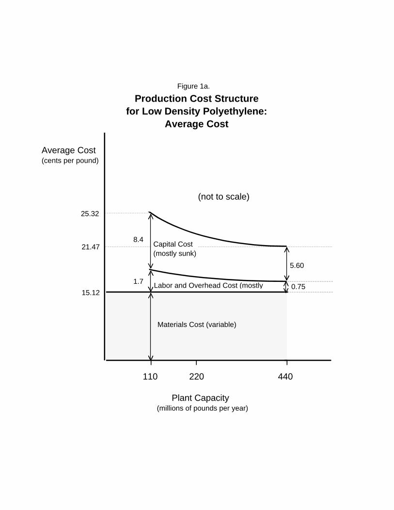
Figures 1a and 1b illustrate the cost structure for a specific product, low-density

polyethylene (LDPE). The mid-size LDPE plant listed in the Yearbook was capable of

producing 220 million pounds per year, while the smaller and larger plants had capacities

of 110 million and 440 million pounds per year, respectively. (There is typically a

doubling of capacity between the plant sizes reported.) The unit materials cost, v, was

15.12 cents per pound, independent of plant size. Other cost categories---capital

investment, labor and overhead---are subject to scale economies. Given these economies,

Figure 1a shows that the estimated average total production cost for LDPE was at 25.32

cents per pound in the smaller plant, falling to 21.47 cents per pound in the larger plant.

Figure 1b, which plots total costs versus plant size, shows how the engineering

cost estimates are mapped into the Dixit function. The bold line at the top of the figure

connects the estimates of total plant investment costs for the smaller plant ($46.3 million),

medium plant ($69.7 million) and larger plant ($123.1 million), as reported in the

Yearbook. Extrapolation back to the y-axis shows that a hypothetical plant of capacity

“zero” would have required a lump-sum investment of $22.9 million. This is equivalent to

an annual investment flow cost of $4.58 million, assuming a 10% cost of capital and 10%

annual depreciation. This flow investment cost for a “zero capacity” plant was taken as

the entry fee, F.11

Figure 1b shows that total investment cost increases in almost-linear fashion with

plant capacity and output, x. Materials costs also grows linearly. Labor costs do not, but

they are a very small fraction of total costs. The measure, SUNKRATIO, equals the ratio

of r/v as shown in the figure. SUNKRATIO is the incremental plant investment cost per

unit of capacity, divided by the materials cost per unit.

11 As an alternative, the total investment cost of the smaller plant ($46.3 million for HDPE) was used as avalue for F. Results were very similar to those reported below. An early version of this paper used a morecomplex parametrization of the cost function, also with similar results.

11

The deterrence models of Dixit and Eaton-Ware suggest that the number of firms

should fall as SUNKRATIO rises. However, SUNKRATIO also corresponds to the wedge

between the Marshallian entry- and exit-inducing prices in the industry. Given a stochastic

entry process arising from uncertainty about demand, technology, costs, or the behavior of

rival firms (c.f., Dixit and Shapiro (1986), Cabral (1993, 1997)), industries with higher

values of SUNKRATIO may tend to exhibit larger numbers of firms. The key test of this

study is to determine whether the net effect of SUNKRATIO is positive, negative or zero

on average.

Many of the early studies of cost structure and concentration attempted to measure

the extent of scale economies based on the slope of the cost function. Such a measure of

scale economies was developed for the present study. SCALECON equals the reduction in

total costs associated with a doubling of capacity. In the case of LDPE, shown in Figure

1a, SCALECON was computed as 1-(21.47/25.32)^.5 = 7.9%. (Larger figures correspond

to greater scale economies.) SCALECON was tested in the regressions to determine

whether the number of producers is sensitive to the slope of the cost function, rather than

the size of the entry fee (F) and incremental sunk costs (SUNKRATIO).

Early studies also found that concentration and entry were sensitive to the size of

the market measured relative to a plant of “minimum efficient scale.” To test this idea, an

additional measure was developed, corresponding to industry output divided by the

capacity of the “mid-size plant,” where the latter is identified in the Yearbook as being

“representative of sizes of competitive U.S. plants.”12

Market Size and Growth

Other things equal, larger markets can sustain more firms. This basic relation is

intuitive and has been identified in virtually all studies on the determinants of producer

concentration. This study controls for differences in market size but includes only limited

12 Alternatively, one might use the size of the smaller plant shown in the Yearbook, but in nearly all casesthis is half the size of the mid-size plant, so the two MES estimates differ by a simple scaling factor.

12

measures of other demand characteristics. Detailed demand-side information is not readily

obtainable for the chemical products in the sample.

The primary demand-side measure used in the study is annual industry output,

which can be measured in either physical or monetary units. Accordingly, two alternate

measures of U.S. market size are included in the regressions: POUNDS (total industry

output, measured by weight), and SALES (monetary value of this output, computed by

multiplying POUNDS by the product’s unit sales value). Data on SALES were recorded

for 1977 only; POUNDS data were collected for 1977, 1987, and a historical period from

the 1960s through 1977.13

Using the historical output data, measures were developed to assess whether

concentration was influenced by the time path of industry growth (controlling for the final

output level). There are various reasons why the growth rate of output, or changes in that

rate, could affect the number of producers. Given increasing marginal costs of adjusting

capacity, rapid demand growth might outstrip incumbent firms’ abilities to expand, thereby

facilitating additional entry (Hause and DuRietz, 1984; Nakao, 1980). Further, the

number of producers may increase with demand volatility. This would arise if supra-

normal profits during peak periods allow the survival of a larger number of firms

(Sheshinski and Dreze, 1977; Mills and Schumann, 1985). Moreover, changes in the rate

of industry growth may lead to uncertainty in entrants’ expectations about the future level

of demand. In industries with hysteresis, this may induce an increase in the number of

producers.14 Ultimately, firms may become trapped in an unprofitable industry if costs are

mostly sunk and there is a large unanticipated downturn in demand.

To assess these potential effects, experiments were performed by adding to the

regressions various measures derived from the historical output data. These measures

included the average recent growth rate of output, the maximum annual rate (post-1960),

the degree of variability in annual output (measured as the residuals from a quadratic

13 The U.S. output data were collected annually for most products back to 1960.14 Uncertainty could also lead to a smaller number of firms, as it may raise the demand or price thresholdnecessary to induce entry.

13

regression of industry output on time), the change in industry growth rate (pre- versus

post-1970) and a dummy for industries with declining demand.15 These measures were

also interacted with SUNKRATIO, given that some of the effects described above would

be expected to increase with the magnitude of sunk costs.

Degree of Multiplant Operation

The SRI engineering data pertain to the cost structure of plants, whereas the

theoretical models are based on the cost structure of firms. If multiplant economies are

important, the assumptions made above regarding the cost parameters may be

inappropriate. A measure of multiplant operation, MULT, was used to determine whether

factors related to multi-plant operation were important determinants of the number of

firms in the sample. MULT equals the average number of plants per firm producing the

product in question in the United States in 1977. A significant MULT coefficient in the

regressions would imply that (unobserved) factors relating to multiplant economies of

scale had an important influence on the number of producers.

Correlations among the Variables

Table 3 gives a matrix of first order correlation coefficients for the variables in the

study. The two measures of market size (SALES and POUNDS) are strongly correlated

with the number of producers, but the cost measures (F, SUNKRATIO, and SCALECON)

are not. These cost measures are, nevertheless, correlated with each other, as all three

tend to be larger for plants with high capital investment. Nevertheless, the three measures

capture different aspects of the cost structure, and their independent effects can be

identified in the regressions. The number of plants per firm, MULT, is positively

correlated with the number of producers, indicating a tendency for greater multiplant

operation in less concentrated markets.

15 Only a few products exhibited declining output prior to 1977, and the extent of these declines wassmall.

14

4. Empirical Results

Table 4 reports the regression results for the number of U.S. producers in 1977,

based on instrumental variable estimation.16 (The OLS results, which are almost identical,

are in the Appendix.) These regressions show that the number of producers was largely

determined by market size and sunk costs.

In regressions 4.1 through 4.5, SALES is used as the measure of market size;

regressions 4.6 through 4.10 use POUNDS. The fit is substantially better with POUNDS,

but the results otherwise are similar. The SALES coefficients are approximately unity,

which implies that the number of producers increased in direct proportion with market

size, measured in monetary terms. The POUNDS regressions yield smaller coefficients but

indicate that differences in market size, measured in physical units, can account for well

over half of the sample variance in the number of producing firms.

The cost measures, F and SUNKRATIO, are highly significant with opposite signs.

The number of producers fell with the entry fee, F. The magnitude of this effect depends

on the specification; the F coefficient doubles in size and the regression fit improves

substantially when SUNKRATIO is included. This suggests that consideration of the entry

fee alone, without the effects represented by SUNKRATIO, leads to a serious

underestimate of the relationship. The dramatic improvement in fit when SUNKRATIO is

added to the specification proved quite robust across time periods and geographic regions.

Regression 4.8 shows that for the U.S. data, more than 80% of the sample variance in the

number of producers can be accounted for by differences in market size and sunk costs.

The coefficient of SUNKRATIO is consistently positive, implying that (after

controlling for F) the number of producers increased with degree to which total costs

were sunk. This is consistent with hysteresis effects, but not entry deterrence or

16 The set of instruments is described in Table 4. Tests showed the absence of heteroskedasticity in thefully specified regression model (e.g., regression 4.8), but to be conservative Table 4 gives t-statisticsbased on robust standard errors. The dependent variable is based upon descrete count data with aminimum bound; the residuals nevertheless appear normally distributed when the variable is in log form.Tobit regression, which takes the bound into account, provided estimates very similar to those in Table 4.

15

preemption. Such evidence is strong but not definitive; conceivably, preemptive behavior

based on sunk cost commitments could have occurred for a limited number of products in

the sample.

Thus, the entry fee and the sunk cost ratio tend to push the market structure in

opposite directions. What, then, is the net effect? Do sunk costs ever lead on balance to

an increase in the number of firms? One way to answer this question is to estimate the

relative influence of the two cost components for each product in the sample. Such

estimates are provided in Figure 2, which was obtained by multiplying the F and

SUNKRATIO coefficients in regression 4.8 by the values corresponding to each data point.

In Figure 2, the horizontal axis gives the reduction in the number of producers attributable

to the entry fee, F; the vertical axis gives the increase in number of producers attributable

to the sunk cost ratio. These two effects exactly offset each other along the dotted

diagonal line.

Nearly all of the 31 products in the sample fall below this diagonal; thus, the net

effect of sunk costs was almost uniformly to reduce the number of firms. The one

exception is maleic anhydride, whose sunk cost ratio was the highest in the sample, but

whose entry fee was only about half the sample average. The regression coefficients imply

that the sunk cost ratio for maleic anhydride, considered alone, served to increase the

number of producers by roughly a factor of four, whereas the entry fee reduced the

number by about a factor of three. Their net effect on the predicted number of firms is

therefore slightly positive.

The other cost measure in Table 4, SCALECON, proved uniformly insignificant in

the regressions when included with F and SUNKRATIO. Similar results (not shown) were

obtained for the measure representing industry output divided by the capacity of a “mid-

size plant.” These findings suggest that the entry fee and sunk cost ratio represent more

suitable constructs than the earlier and less precise concepts of “minimum efficient scale”

and degree of scale economies.

16

Table 4 shows that MULT, the average number of plants per firm, was not

statistically significant. The European data gave similar insignificant results (not shown).

These findings imply that multiplant economies of scale did not play an important role in

determining the number of producers in the industries examined in this study.

Experiments were performed to assess whether the historical growth path of

industry output had an influence on the number of firms. The results of these experiments

were negative; the output growth and variability measures were uniformly insignificant

when added to Regression 4.8 and related specifications. Interactions with SUNKRATIO

were also statistically insignificant. Thus there was no evidence that rapid growth or

substantial variability in (annual) demand contributed to an increase in the number of

firms. In general, the effects of cost structure on the number of competitors appeared

remarkably robust to differences in the profile of industry growth. (NOTE: A table of

regression results can be added here, and the discussion expanded.)

If unanticipated shifts in demand were not the primary source of hysteresis effects,

what may have led to “excess” entry? In the chemical industry, expectations about costs

are likely to have been more important than demand-side factors. Many firms entered in

anticipation of attaining cost advantages, based upon potentially superior (newer)

technology or access to low-cost inputs. In cases where these expectations were not

borne out, but sunk costs were high, entrants would have persisted in the industry despite

their inability to cover total costs. And even when entrants did attain a cost advantage,

incumbents’ plants would have continued to operate, assuming that prices remained above

variable costs.

A further regression analysis was performed to determine whether the observed

relationships were robust across geographic markets and over time. To supplement the

results for 1977, the model (represented by regression 4.8) was estimated for the number

of U.S. producers in 1967 and 1987, as well as for producers in Europe and Japan. These

regression results are shown in Table 5.

17

For the United States, the 1967 and 1987 regression estimates are similar to those

for 1977 discussed previously. The coefficients and fit obtained for 1977 and 1987 are

nearly identical; for 1967 the fit is slightly poorer and coefficient estimates smaller.

Weaker results would be expected for this earlier period, given errors that arise in

applying the 1977 cost parameters to the 1967 data. In general, though, these results

imply that the relationships identified in Table 4 were robust over time.

Table 5 also shows that the regression results for Western Europe resemble those

for the United States. The Japanese results are also comparable, despite the smaller

Japanese sample. Regression 5.5 suggests that the influence of cost structure was weaker

in Japan in 1977 than in the other regions. This may be due to MITI’s role in regulating

entry through the mid-1970s. The effects of sunk costs appear more prominent in the

Japan regression for 1989; here, the coefficients and R2 approach the values shown for the

U.S. and Europe.

5. Conclusions

Using a unique set of engineering data, this study has examined factors that

potentially determine the number of competitors in a homogeneous product industry. The

results show that producer concentration in the sample of 31 chemical product industries

was largely determined by market size and the structure of sunk costs. The findings are

similar for the three geographic regions---United States, Western Europe and Japan---and

robust over time.

The two measures of sunk cost identified in this study appear to have had

substantial but opposite effects. A larger entry fee led to higher producer concentration,

while increases in the ratio of sunk to variable costs led to an increase in the number of

firms. The latter findings are consistent with hysteresis effects, but not with strategic

preemption or entry deterrence.

These findings help to resolve ambiguities raised by prior theoretical and empirical

work on sunk costs. They imply that it is important to distinguish between the entry fee

18

and incremental components of sunk cost. Otherwise, empirical studies will tend to

underestimate the impact of each component on market structure and potentially

misinterpret their net effect.

In addition to the entry fee and sunk cost ratio, measures were developed in this

study resembling those in the earlier literature on scale economies. These measures were

found to lack explanatory value. Such findings suggest that the entry fee and sunk cost

ratio, which have links with modern economic theory, are more suitable constructs than

the earlier but less precise concepts of “minimum efficient scale” and cost curve slope.

The findings also suggest that the dynamics of industry growth have little effect on

market structure. While the number of chemical producers was strongly related to the

current level of industry output, no connection was found between concentration and the

historical path of output. Thus the rate and variability of industry growth had no

significant impact on the number of firms. This suggests that adjustment costs and related

factors have been relatively unimportant, at least in chemical product industries.

These results must be generalized with caution given the small sample size.

Moreover, it should be emphasized that the findings are specific to homogeneous product

industries. Sutton’s (1991) recent work suggests that sunk costs play a greater role in

promoting concentration in differentiated product industries, where sunk investments are

mostly in intangible assets such as advertising and R&D. Such costs can potentially grow

without bound. In chemicals and other mature homogeneous product industries, sunk

costs are inherently tied to production capacity, which limits their extent.

19

REFERENCES

Arora, A., and A. Gambardella (1998). Evolution of Industry Structure in the ChemicalIndustry. Chemicals and Long-Term Economic Growth. A. Arora, R. Landau and N.Rosenberg. New York, Wiley: 379-414.

Asplund, M., and R. Sandin (1999). “The Number of Firms and Production Capacity inRelation to Market Size.” The Journal of Industrial Economics XLVII(1): 69-85.

Bain, J. S. (1956). Barriers to New Competition. Cambridge, Mass., Harvard UniversityPress.

Baldwin, R. E. (1988). “Hysteresis in Import Prices: The Beachhead Effect.” AmericanEconomic Review 78(4): 773-785.

Berry, S. (1992). “Estimation of a model of entry in the airline industry.” Econometrica60(4): 889-917.

Bresnahan, T. F., and P. C. Reiss (1990). “Entry in Monopoly Markets.” Review ofEconomic Studies 57: 531-553.

Bresnahan, T. F, and P. C. Reiss (1991). “Entry and Competition in ConcentratedMarkets.” Journal of Political Economy 99: 977-1009.

Bresnahan, T. F., and P. C. Reiss (1993). “Measuring the Importance of Sunk Costs.”Annales D'Economie et de Statistique 31: 181-217.

Cabral, L. (1993). “Experience Advantages and Entry Dynamics.” Journal of EconomicTheory 59: 403-416.

Cabral, L. (1997). “Entry Mistakes.” Discussion Paper #1729, Center for Economic PolicyResearch, London.

Curry, B., and K. D. George (1983). “Industrial Concentration: A Survey.” Journal ofIndustrial Economics 31(3): 203-255.

Dixit, A. (1980). “The Role of Investment in Entry-Deterrence.” The Economic Journal90: 95-106.

Dixit, A. (1989). “Entry and Exit Decisions Under Uncertainty.” Journal of PoliticalEconomy 97(3): 620-638.

Dixit, A. and C. Shapiro (1986). “Entry Dynamics with Mixed Strategies.” In L.Thomas, ed., The Economics of Strategic Planning. Lexington Books, 63-79.

20

Dunne, T., M. J. Roberts and L. Samuelson (1988). “Patterns of Firm Entry and Exit inU.S. Manufacturing Industries.” Rand Journal of Economics 19(4, Winter): 495-515.

Dunne, T., M. J. Roberts and L. Samuelson (1989). “Firm Entry and Post-EntryPerformance in the U.S. Chemical Industries.” Journal of Law and Economics 32(2):S233-S275.

Eaton, B. C., and Ware, R. (1987). “A Theory of Market Structure with SequentialEntry.” Rand Journal of Economics 18: 1-16.

Freeman, C. (1968). “Chemical Process Plant Innovation and the World Market.” NationalInstitute Economic Review 45: 29-51.

George, K., and T. S. Ward (1975). The Structure of Industry in the EEC. Cambridge,Cambridge University Press.

Ghemawat, P., and R. E. Caves (1986). “Capitial Commitment and Profitability: AnEmpirical Investigation.” Oxford Economic Papers 38: 94-110.

Gilbert, R. J. (1986). Pre-emptive Competition. New Developments in the Analysis ofMarket Structure. J. E. Stiglitz and G. F. Mathewson. Cambridge, MIT Press.

Hause, J. C., and G. du Rietz (1984). “Entry, Industry Growth, and the Microdynamics ofIndustry Supply.” Journal of Political Economy 92: 733-757.

Heavy & Chemical Industries News Agency of Japan (annual). Annual Survey ofPetrochemical Industries in Japan (Jukagaku Kogyo Tsushin-sha, Nihon no SekiyuKagaku Kogyo, in Japanese). Tokyo, The Heavy & Chemical Industries News Agency.

Hikino, T., T. Harada, Y. Tokuhisa and J. Yoshida (1998). The Japanese Puzzle.Chemicals and Long-Term Growth: Insights from the Chemical Industry. A. Arora, R.Landau and N. Rosenberg. New York, Wiley.

Kessides, I. N. (1990). “Market Concentration, Contestability, and Sunk Costs.” Reviewof Economics and Statistics: 614-622.

Klepper, S., and E. Graddy (1990). “The Evolution of New Industries and theDeterminants of Market Structure.” Rand Journal 21(Spring): 27-44.

Lieberman, M. B. (1987). “Excess Capacity as a Barrier to Entry: An EmpiricalAppraisal.” Journal of Industrial Economics 35(June): 607-627.

MacLeod, W. B. (1987). “Entry, Sunk Costs, and Market Structure.” Canadian Journal ofEconomics 20(1): 140-151.

21

Mills, D. E., and L. Schumann (1985). “Industry Structure with Fluctuating Demand.”The American Economic Review 75(September): 758-767.

Nakao, T. (1980). “Demand Growth, Profitability, and Entry.” Quarterly Journal ofEconomics 94(March): 397-411.

Pashigian, P. (1969). “The Effect of Market Size on Concentration.” InternationalEconomic Review 10(October): 291-314.

Pryor, F. L. (1972). “An International Comparison of Concentration Ratios.” The Reviewof Economics and Statistics LIV: 130-140.

Reiss, P. C., and P. Spiller (1989). “Competition and Entry in Small Airline Markets.”Journal of Law and Economics 32(Supplement): 179-202.

Scherer, F. M. (1973). “The Determinants of Industrial Plant Sizes in Six Nations.” TheReview of Economics and Statistics LV(May): 135-145.

Spitz, P. H. (1988). Petrochemicals: The Rise of an Industry. New York, Wiley.

SRI International (1976). Process Economics Program Yearbook. Menlo Park, CA. SRIInternational.

SRI International (1989). Directory of Chemical Producers, Western Europe. Menlo Park,CA, SRI International.

SRI International (annual issues). Directory of Chemical Producers, United States. MenloPark, CA, SRI International.

Stobaugh, R. (1988). Innovation and Competition: The Global Management ofPetrochemical Products. Boston, Harvard Business School Press.

Sutton, J. (1991). Sunk Costs and Market Structure: Price Competition, Advertising, andthe Evolution of Concentration. Cambridge, Mass., MIT Press.

W. Europe

1960 1967 1977 1987 1989 1977 1989

Acetic Acid * 6 7 6 17 7 8Acetone * 11 14 13 14 6 6Acrylonitrile 4 5 4 5 9 6 6Adipic Acid * 6 5 3 6 * *Ammonia 40 64 57 43 38 * *Aniline 4 5 5 5 7 * *Bisphenol A 3 5 4 4 6 2 3Caprolactam 1 4 3 3 8 4 4Cumene * 10 12 10 10 * *Cyclohexane 3 12 9 6 8 7 7Ethylbenzene * 14 15 9 15 * *Ethylene 20 20 26 23 34 14 12Ethylene Glycol 9 12 11 10 13 * *Formaldehyde 14 15 18 15 58 * *Hydrogen Peroxide * 6 6 3 19 * *Isopropyl Alcohol 3 4 4 4 7 3 3Maleic Anhydride 4 7 8 5 13 5 6Methanol 9 12 10 12 7 7 5Methyl Methacrylate 2 4 3 3 7 * *Nitric Acid * 47 49 43 47 * *Phenol 9 12 11 12 10 2 5Phthalic Anhydride 9 12 9 5 17 7 6Polyethylene-HD 8 11 12 15 20 10 10Polyethylene-LD 9 9 13 12 27 10 10Polypropylene Resins * 9 9 12 25 10 14Polystyrene Resins * * 18 19 31 8 9Propylene Glycol * 8 5 5 8 5 5Styrene 8 11 11 8 12 9 7Urea 12 34 33 28 23 * *Vinyl Acetate 4 7 6 4 5 9 5Vinyl Chloride 12 12 10 8 19 17 11

AVERAGE 8.9 13.1 13.1 11.4 17.4 7.4 7.1

*Data not available.

Sources: Directory of Chemical Producers, United States (1960, 1967, 1977, 1987); Directory of Chemical Producers, Western Europe (1989); Annual Survey of Petrochemical Industries in Japan (1977, 1989).

United States Japan

Table 1.

Number of Producers

U.S. (1977) U.S. (1987) W.Europe (1989) Japan (1977)

U.S. (1977) 1.00

U.S. (1987) .98 1.00

W.Europe (1989) .71 .73 1.00

Japan (1977)* .55 .47 .63 1.00

Japan (1989)* .61 .64 .84 .81

*Sample of 31 products for U.S. and W. Europe; 20 products for Japan.

Table 2.

Correlations Between Numbers of Producers:U.S., Western Europe and Japan

Mean Std Dev Minimum Maximum

log NFIRMSUS,1977 2.28 0.74 1.10 4.04

log SALES 6.11 0.90 4.28 8.01

log POUNDS 7.85 1.25 5.23 10.48

log F 2.87 0.80 1.44 4.57

SUNKRATIO 0.28 0.19 0.03 0.74

SCALECON 0.06 0.04 0.01 0.14

MULT 1.38 0.38 1.00 3.00

log NFIRMS log SALES log POUNDS log F PCTSUNK SCALECON

log NFIRMSUS,1977 1.00

log SALES 0.63 1.00

log POUNDS 0.81 0.88 1.00

log F 0.10 0.58 0.38 1.00

SUNKRATIO 0.05 -0.05 -0.13 0.48 1.00

SCALECON -0.02 -0.18 -0.25 0.24 0.85 1.00

MULT 0.42 0.16 0.32 -0.17 -0.02 0.16

Table 3

Correlation Matrix of Explanatory Variables

Table 4.

Regression Analysis of Number of U.S. Producers in 19771

4.1 4.2 4.3 4.4 4.5 4.6 4.7 4.8 4.9 4.10

constant -1.32 -1.57 -2.49 -2.52 2.35 -1.55 -1.36 -1.89 -1.86 -2.37(-1.8) (-1.9) (-3.5) (-5.8) (0.4) (-2.4) (-2.1) (-5.4) (-7.6) (-0.6)

log SALES .59 .84 1.08 1.06 .94(5.0) (5.7) (7.7) (10.0) (9.7)

log POUNDS .49 .55 .65 .66 .66(6.2) (6.0) (12.2) (9.5) (9.1)

log F -.46 -.87 -.84 -.77 -.24 -.50 -.51 -.51(-2.9) (-6.6) (-6.2) (-6.0) (-2.8) (-6.3) (-5.5) (-5.4)

SUNKRATIO 2.30 2.25 2.80 1.83 1.86 1.78(4.3) (3.9) (2.7) (5.5) (4.4) (2.2)

SCALECON -4.43 .50(0.9) (0.1)

MULT .07 .22 -0.5 -0.7(0.6) (1.5) (-0.2) (-0.3)

R2 .391 .495 .633 .640 .662 .649 .701 .828 .828 .828__

R2 .370 .459 .592 .585 .594 .637 .680 .809 .801 .793

No. of Obs. 31 31 31 31 31 31 31 31 31 31

1 Dependent variable is the logarithm of the number of United States producers in 1977. Regressions were estimated using instrumental variables for SALES,POUNDS and MULT, which are potentially endogenous. The set of instruments includes total counts of Western European producers, plants and capacity in1989, and national counts of plants and producers in France, Germany, Italy and the UK. Numbers in parentheses are heteroskedastic-consistent t-statistics.

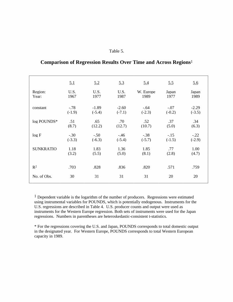
Table 5.

Comparison of Regression Results Over Time and Across Regions1

5.1 5.2 5.3 5.4 5.5 5.6

Region: U.S. U.S. U.S. W. Europe Japan JapanYear: 1967 1977 1987 1989 1977 1989

constant -.78 -1.89 -2.60 -.64 -.07 -2.29(-1.9) (-5.4) (-7.1) (-2.3) (-0.2) (-3.5)

log POUNDS* .51 .65 .70 .52 .37 .34(8.7) (12.2) (12.7) (10.7) (5.0) (6.3)

log F -.30 -.50 -.46 -.38 -.15 -.22(-3.3) (-6.3) (-5.4) (-5.7) (-1.5) (-2.9)

SUNKRATIO 1.18 1.83 1.36 1.85 .77 1.00(3.2) (5.5) (5.0) (8.1) (2.8) (4.7)

R2 .703 .828 .836 .820 .571 .759

No. of Obs. 30 31 31 31 20 20

1 Dependent variable is the logarithm of the number of producers. Regressions were estimatedusing instrumental variables for POUNDS, which is potentially endogenous. Instruments for theU.S. regressions are described in Table 4. U.S. producer counts and output were used asinstruments for the Western Europe regression. Both sets of instruments were used for the Japanregressions. Numbers in parentheses are heteroskedastic-consistent t-statistics.

* For the regressions covering the U.S. and Japan, POUNDS corresponds to total domestic outputin the designated year. For Western Europe, POUNDS corresponds to total Western Europeancapacity in 1989.

(not to scale)

Labor and Overhead Cost (mostly

110 220 440

15.12

25.32

21.47

Plant Capacity (millions of pounds per year)

Average Cost (cents per pound)

Production Cost Structurefor Low Density Polyethylene:

Average Cost

5.60

0.751.7

8.4Capital Cost (mostly sunk)

Figure 1a.

Materials Cost (variable)

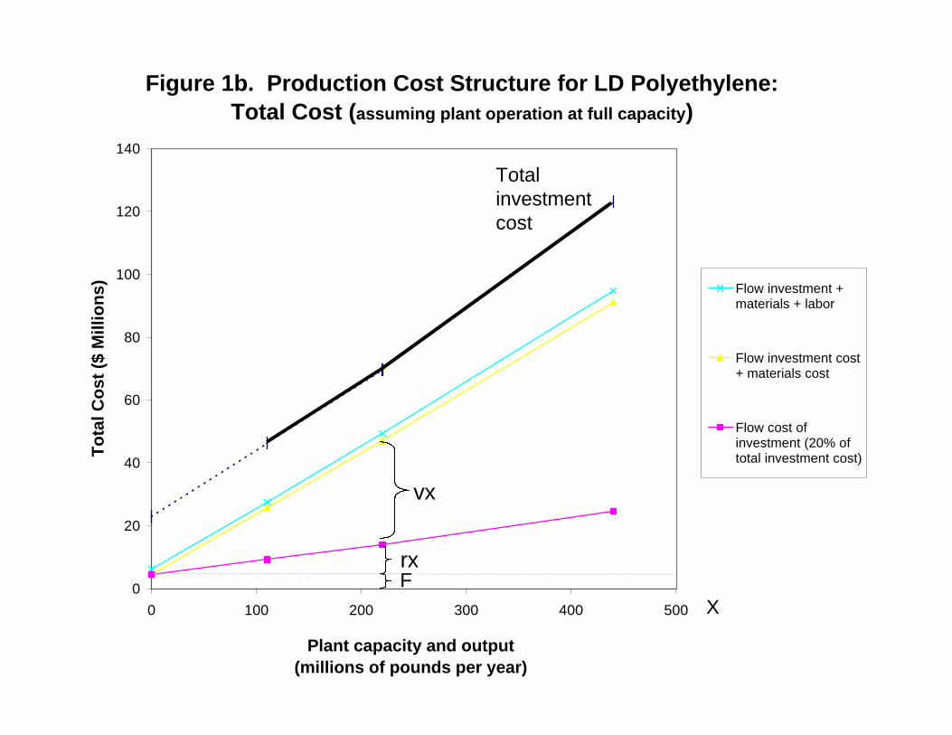
Figure 1b. Production Cost Structure for LD Polyethylene: Total Cost (assuming plant operation at full capacity)

0

20

40

60

80

100

120

140

0 100 200 300 400 500

Plant capacity and output (millions of pounds per year)

To

tal C

ost

($

Mill

ion

s) Flow investment +materials + labor

Flow investment cost+ materials cost

Flow cost ofinvestment (20% oftotal investment cost)

FF

vx

X

rx

Total investment cost

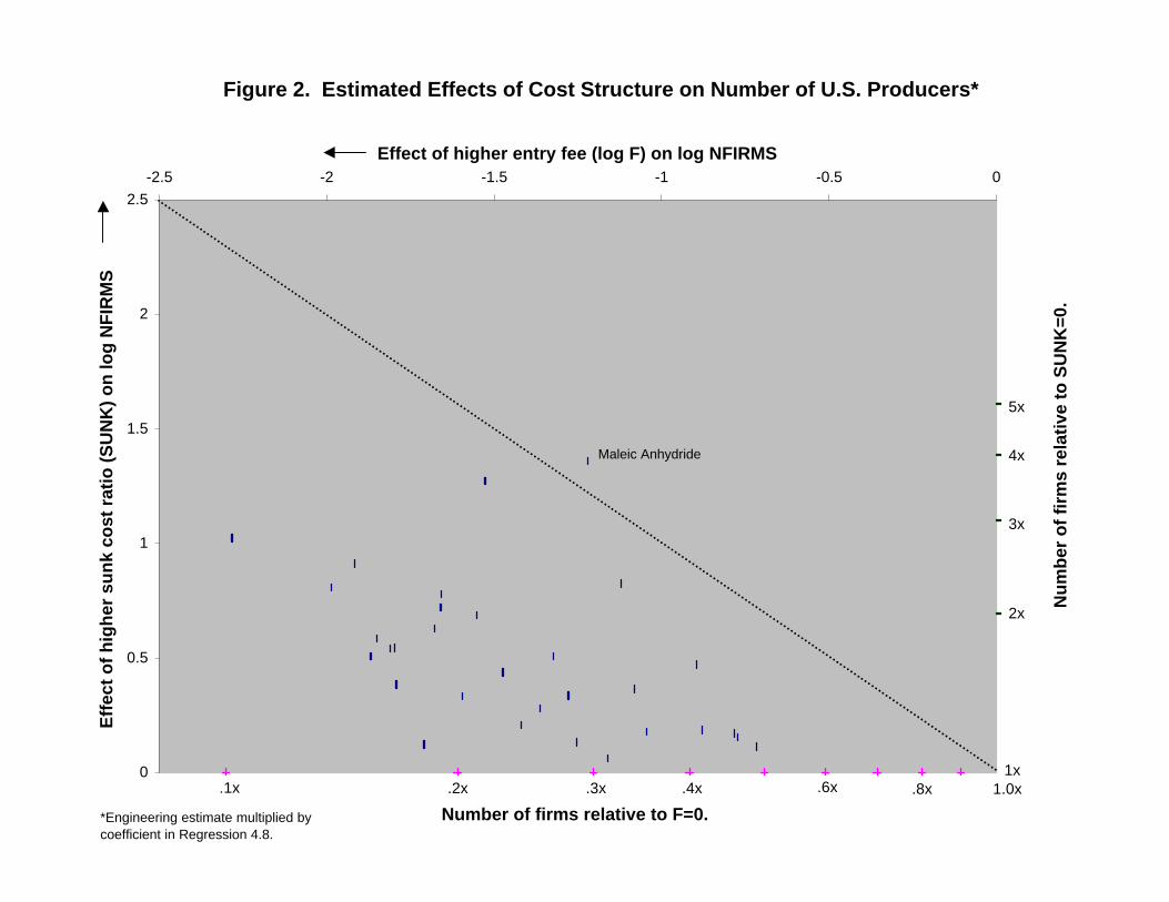
Figure 2. Estimated Effects of Cost Structure on Number of U.S. Producers*

0

0.5

1

1.5

2

2.5

-2.5 -2 -1.5 -1 -0.5 0

Effect of higher entry fee (log F) on log NFIRMS

Eff

ect

of

hig

her

su

nk

cost

rat

io (

SU

NK

) o

n lo

g N

FIR

MS

.1x

Number of firms relative to F=0.

Nu

mb

er o

f fi

rms

rela

tive

to

SU

NK

=0.

2x

1x

3x

1.0x.8x

4x

5x

.2x .3x .4x .6x

*Engineering estimate multiplied by coefficient in Regression 4.8.

Maleic Anhydride