WHAT CAUSED CHICAGO BANK FAILURES IN THE GREAT DEPRESSION ... 22 (Postel-Vinay, April 20… ·...

Working Paper No. 22 – 2015:

WHAT CAUSED CHICAGO BANK FAILURES IN THE GREAT

DEPRESSION? A LOOK AT THE 1920s.

Natacha Postel-Vinay University of Warwick

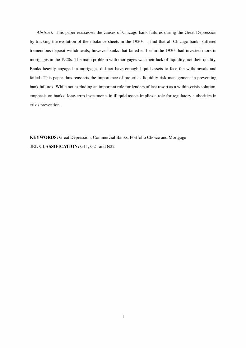
Abstract: This paper reassesses the causes of Chicago bank failures during the Great Depression

by tracking the evolution of their balance sheets in the 1920s. I find that all Chicago banks suffered

tremendous deposit withdrawals; however banks that failed earlier in the 1930s had invested more in

mortgages in the 1920s. The main problem with mortgages was their lack of liquidity, not their quality.

Banks heavily engaged in mortgages did not have enough liquid assets to face the withdrawals and

failed. This paper thus reasserts the importance of pre-crisis liquidity risk management in preventing

bank failures. While not excluding an important role for lenders of last resort as a within-crisis solution,

emphasis on banks’ long-term investments in illiquid assets implies a role for regulatory authorities in

crisis prevention.

KEYWORDS: Great Depression, Commercial Banks, Portfolio Choice and Mortgage

JEL CLASSIFICATION: G11, G21 and N22

1

1 Introduction

The recent financial crisis has raised significant questions about the causes of bank failures. While

many thought that deposit insurance would prevent the incidence of bank runs and thus induce only

insolvent banks to fail, bank runs did in fact occur (on uninsured liabilities) and greatly worsened the

crisis. The question as to whether banks fail primarily because of reckless investments or because

of funding illiquidity has thus once again been at the centre of debates, with strong implications for

government policy (Bordo & Landon-Lane, 2010; Brunnermeier, 2008; Calvo, 2013; Gorton & Metrick,

2013; Kacperczyk & Schabl, 2010; Reinhart, 2011; Shin, 2009; Schleifer & Vishny, 2011; Stein, 2013).

On the one hand, it is commonly believed that if banks’ asset quality is low (giving rise to low

repayment probabilities on banks’ investments), there is no good reason for the government to intervene.

Providing them with emergency liquidity will not solve their solvency problem, and bailing them out

will likely lead them to take more risks than is collectively desirable. On the other hand, if banks face

large withdrawals despite high-quality investments (with high ex ante probabilities of repayment), their

failure is usually viewed as unjustified – suggesting a role for government intervention in the form of

liquidity provision by the central bank.

The aim of this paper is to answer this question with respect to one of the deepest financial crises in

modern times – the U.S. Great Depression. More specifically, it focuses on the city of Chicago, which

had one of the highest urban bank failure rates in the country.1 Although other authors have focused on

Chicago, this paper’s method departs from previous research along three dimensions. First, I introduce

a novel way of examining Chicago state bank failures by separating them into three cohorts ordered

through time: June 1931 failures, June 1932 failures and June 1933 failures, each corresponding to six-

month failure windows containing both panic and non-panic failures. Second, rather than focusing on

banks’ 1929 balance sheets, I look at the evolution of survivors and failures during the full decade from

1923 all the way up to 1933. Third, I specifically examine the relative importance of each financial ratio

in predicting failure.

This third methodological input seems particularly important, as recent balance sheet studies of De-

pression bank failures usually have not specifically focused on the comparative significance of each

balance sheet ratio. Rather, they have concentrated on examining whether any pre-Depression ratios

could together successfully predict bank failure. Such balance sheet studies naturally emerged in re-1Out of 193 state banks in June 1929, only 35 survived up to June 1933.

2

sponse to Friedman & Schwartz (1963)’s work, which by analyzing banking aggregates suggested that

banks failed through no fault of their own, having to face mass deposit withdrawals in a series of bank-

ing panics. The idea behind balance sheet studies was to ask whether any pre-Depression balance sheet

items could predict failure, in which case banks should better be seen as “weak” ex ante (White, 1984;

Calomiris & Mason, 1997, 2003; Esbitt, 1986; Guglielmo, 1998; Thomas, 1935).

Such studies have greatly advanced our state of knowledge on the causes of bank failure in the

Great Depression by showing that many banks indeed presented major weaknesses prior to their failure.

Nevertheless, an important feature common to many of them was that these weaknesses were not always

clearly defined. They usually included a range of possible acts of negligence on the part of banks, from

the setting of low capital ratios to overinvestment in long-term loans to the maintenance of low cash

reserves.2

Some of these items are in fact linked to banks’ liquidity, not just to the quality of their investment

(ie. not just to their probability of default). For example, the importance of cash holdings in predicting

bank failure is obviously linked to banks’ capacity to meet cash withdrawals. Likewise, long-term loans

can be riskier from a liquidity point of view, because of the increased maturity mismatch. Some balance

sheet items are intrinsically more liquid than others, regardless of their quality. In other words, if the best

predictors of failure ex ante happen to be assets whose intrinsic liquidity matters, banks’ weaknesses can

be more clearly specified as resulting from liquidity mismanagement.

Differentiating between credit risk management and liquidity risk management seems important

when tackling Friedman and Schwartz’s argument that the banks that failed were simply “illiquid,” and

thus failed unjustifiably. Of course, banks are by nature illiquid to some extent, due to their important

role in maturity transformation.3 But if banks face depositor runs, aren’t those that are the most prepared

for such runs, that is, those that most attended ex ante to their portfolio’s inherent liquidity, more likely

to survive? The question may not arise in a world of deposit insurance, where runs are supposed to be

unlikely. Nevertheless, the recent crisis has shown that runs can occur on uninsured parts of the banking

system (Brunnermeier, 2008; Gorton & Metrick, 2013). Moreover, deposit insurance can increase moral

hazard by inducing banks to take on more credit risk, which itself would potentially lead to a greater2In some cases it was not always clear whether banks’ failure was deemed to be mainly the result of bank mismanagement

in setting certain ratios or the result of a general fall in certain asset values, or both. For example, if the variable “other loansto total assets” was significant, it was sometimes unclear whether banks should be blamed for having too many of such loans,or if a general recession caused a fall in the value of those loans regardless of banks’ actions, or both.

3In addition, banks may find themselves particularly illiquid due to freezing markets during crises in which investors doubtthe quality of certain assets and refuse to buy them at their original price.

3

risk of a run on uninsured items.

This paper’s principal finding is that real estate loan holdings are the best predictor of failure as well

as of timing of failure. Examining cohorts of bank failures graphically through time, it appears that they

are most clearly ordered in terms of their mortgage holdings: the higher a bank’s amount of mortgages,

the earlier it failed. The ordering is not so clear for other items (such as capital, reserves, stocks and

bonds, and other loans). This is confirmed econometrically by an ordered logistic model, which suggests

that mortgages have the largest predictive power.

At the same time, this paper also shows that all cohorts suffered tremendous deposit withdrawals

throughout the period, including survivors. It therefore emphasizes mortgages’ inherent lack of liquidity

as a determinant risk factor. The quality of mortgages cannot have mattered significantly, for three

reasons. First, most mortgages had a 50 percent loan-to-value (LTV) ratio, while land values did not

fall by more than 50 percent in Chicago until 1933. This means that banks cannot have incurred any

significant losses on defaulting loans. Second, although mortgages had short contract maturities (three to

five years), most of these loans were renewed in good times, creating renewal expectations and increasing

their de facto maturity. Long maturities, the absence of secondary markets and the inability for these

loans to be rediscounted at the Federal Reserve meant that they were inherently less liquid than other

types of loans. Third, I show that sectoral differences in land values within Chicago did not have a

differential impact on bank failure rates.

The view that illiquid assets were the cause of the crisis is supported by evidence that all banks

engaged in fire sales. In this process, mortgages could not be liquidated. Indeed, real estate loans

increased as a share of total assets for all banks during the Depression, at the same time as assets as a

whole were declining. Other types of loans, such as loans on collateral security and “other loans,” were

promptly liquidated.

It is not the aim of this paper to find the origins of deposit withdrawals in Chicago during the

Depression. Two kinds of explanation have usually been put forward. On the one hand, Diamond &

Dybvig (1983) describe them as being caused by depositors either observing a sunspot or suddenly

needing an increased amount of cash.4 On the other hand, Calomiris & Kahn (1991) see bank runs as

a form of monitoring: unable to costlessly value banks’ assets, depositors observing a specific shock to

those assets use runs to reveal the weakest banks.5 In Chicago, depositors in theory could know which4Note that this increased need for cash could be one of the consequences of the Depression.5By “weak,” they imply that banks suffered a shock to the quality and value of their assets.

4

banks had the highest amounts of mortgages thanks to official publications of balance sheet summaries

every six months. This suggests that the cause of those mass withdrawals is indeed still to be determined.

In terms of the consequences of those runs, the interpretation presented in this paper contrasts with

Diamond and Dybvig’s, in which bank runs are usually undesirable phenomena causing even “healthy”

banks to fail. Although in their view “healthy” usually means “solvent,” I suggest that a solvent but

particularly illiquid bank ex ante is not necessarily healthy.

Such findings suggest significant policy implications from a regulatory point of view. While not

excluding an important role for lenders of last resort as a within-crisis solution, emphasis on banks’

long-term investments in illiquid assets implies a role for regulatory authorities in crisis prevention.

Such regulatory measures may include, for instance, renewed emphasis on cash ratios or other liquidity

requirements. This is all the more important given that central banks cannot always precisely predict the

quality of banks’ collateral (especially in the case of assets maturing at a much later date), making their

task a highly complex (and thus possibly imperfect) one (Goodhart, 2010).

Making banks responsible for their liquidity risk management – not just for their credit risk man-

agement – is an idea that has only taken hold in the past few years (Goodhart, 2008). While it was

considered an important aspect of bank regulation from the nineteenth century to the early twentieth

century in the U.S., it was then more or less abandoned, to be replaced by a much more pressing focus

on credit risk, and, in particular, capital requirements, since the 1980s. Liquidity requirements were

indeed almost absent from the Basel I and Basel II regulations, and only recently made a comeback in

the Basel III regulations.6

The results of this paper also suggest a reassessment of the role of real estate in the Great Depression.

Chicago is well-known for its real estate boom in the 1920s, one that resembled both in character and

magnitude the suburban real estate booms of some of the major cities of the American East North

Central and Middle-Atlantic regions.7 Given that the former region had one of the highest numbers of

suspensions in the U.S., the close connection between bank failures and the real estate booms seems

worth investigating.8 The link between real estate and the Depression is probably not a direct one, in the6However it is important to note that so-called liquidity-coverage ratios can lead to some confusion and to regulatory

arbitrage due to their complexity. Perhaps focusing on simple cash ratios would be a better alternative.7These were commonly used census regions. The Chicago boom can be compared in particular to those of Detroit, Pitts-

burgh, Philadelphia (see Wicker, 1996, pp. 16,18), and Toledo (Messer-Kruse, 2004). See also Allen (1931).8The East North Central region (which contains Chicago) had 2,770 suspensions in total between 1930 and 1933 (the term

“suspension” refers to temporary or permanent bank failure, as opposed to “failure” which refers only to the latter category).Only the agricultural states of the West North Central region surpass this number with a total of 3,023 suspensions (Boardof Governors of the Federal Reserve System, 1937, p. 868). Note that the state of Pennsylvania also had a particularly highfailure rate (ibid.).

5

sense that the direct contribution of real estate to the decline in economic activity was small. A number

of recent papers have demonstrated that, in the aggregate, the role of real estate in the Great Depression

was indeed minor.9 This paper assesses the indirect, probably larger contribution that real estate made

to the deepening of the Great Depression via the banking channel. Analysis of the second largest city

in the U.S. in 1930 points to a powerful relationship between real estate lending and commercial bank

failures in the Great Depression.10

Section 2 reviews the literature on banks’ fundamental troubles during the U.S. Great Depression.

Section 3 introduces the data and empirical approach adopted in this study. Section 4 presents empirical

results on the relative importance of financial ratios and on deposit losses. Section 5 focuses on the role

of mortgages’ illiquidity in the crisis. Section 6 concludes.

2 Literature review

This section provides a more precise overview of the literature on the Great Depression. The seminal

work on the Depression was undoubtedly that of Friedman & Schwartz (1963), who emphasized a

“contagion of fear” among depositors, which spread throughout the country after the failure of Bank of

United States in New York City in December 1930. According to this view, mass deposit withdrawals

occurred in a series of four banking panics until Roosevelt called a national bank holiday in March 1933.

The money supply fell by one-third, due to a decrease in the deposit-currency ratio, which led to fire

sales of securities and eventually to the failure of thousands of banks. The Federal Reserve’s role was

seen as crucial in this interpretation, since it generally failed to increase the amount of liquidity available

in the system (see also Wheelock (1991) and Wicker (1996)). In a similar vein, Richardson & Troost

(2009) found that the more expansionary policies characterizing the Atlanta Federal Reserve Bank led

to lower bank failure rates in its District than the more timid policies of the St Louis District in the same

state, Mississippi (see also Richardson (2007)).

Following in the footsteps of Temin (1976), White (1984), on the other hand, compared the balance

sheets of the national banks that failed during the first banking crisis (November-December 1930) with

those of the banks that survived.11 He found that as far back as 1927 many financial ratios determined9See, in particular, White (2009), and Field (2013).

10Chicago was home to 3,376,438 dwellers in 1930, as compared to New York City’s population of 6,930,446 (Carter et al.,2006, Series Aa1-5).

11National banks accounted for only 12.4 percent of all suspensions, whereas state member and non-member banks madeup 2.4 percent and 85.2 percent of all suspensions, respectively. Member banks are members of the Federal Reserve System,

6

banks’ survival. He concluded that the similarities between coefficients from year to year meant that the

causes of failure did not change significantly as banks entered the Depression. This study thus delivered

crucial results as to the possibility of banks’ fundamental troubles, and presented important information

regarding the continuity of banks’ conditions from the onset of the slump up to and including the first

banking crisis.12

Calomiris & Mason (2003) analysed a panel of 8,707 member banks (out of 24,504 banks in total)

from 1929 to 1933, using data on individual banks at two points in time, namely December 1929 and

December 1931. They applied a survival duration model which allowed various variables (including

aggregate and regional economic indicators) to determine chances and length of survival for each bank

at various points in time. They concluded that the financial ratios indeed determined the length of

survival, at least for the first two Friedman-Schwartz crises (late 1930 and March-August 1931). The

only real exception was the fourth banking crisis (early 1933) which “saw a large unexplained increase

in bank failure risk” (ibid.).

The majority of regional balance sheet studies (four in total) have concentrated on Chicago due

to the outstanding magnitude of the Chicago failure rate. The two oldest studies used very similar

methods and obtained similar results. While Thomas (1935) compared the June 1929 balance sheets of

survivors with 1931 failures, Esbitt (1986) analysed the 1927, 1928 and 1929 portfolios of 1930, 1931

and 1932 failures. Both found that, in general, failures had more loans on real estate, had accumulated

smaller surpluses, had fewer secondary reserves and had invested more in bank building. More recently,

Calomiris & Mason (1997) found that banks failing during the summer 1932 crisis had more in common

with other banks failing earlier in 1932 than with survivors, thereby suggesting that widespread depositor

fear was not the primary cause of failure. These banks, in particular, had lower ratios of reserves to

demand deposits, lower ratios of retained earnings to net worth, and higher proportions of long-term

debt in December 1931. The also lost more deposits in 1931. Finally, Guglielmo (1998) compared

the June 1929 balance sheets of both Chicago and Illinois survivors with all Depression failures, using

and a bank suspension occurs when a bank is temporarily or permanently closed, as opposed to a failure which occurs whena bank will permanently close and receivers take control of it to dissolve it. White excluded suspended banks that reopenedas they represented only a small proportion (White, 1984). Note also that White affirms that the causes of failure of state andnational banks were generally similar, as they competed strongly with one another in almost all parts of the country (ibid.).

12White also drew attention to “swollen loan portfolios” and their link to agriculture. Although he did this informally, heexplained that the banks that failed in 1930 were in agricultural areas which suffered from the post- World War I agriculturalland boom and bust. Note that the links between the November 1930 failure of Caldwell and Company, the investment bankinggiant of the South, and the agricultural failures that followed still needs to be assessed. For more information on this bank seeMcFerrin (1939).

7

similar methods, and drew very similar conclusions.13

Some studies have also emerged focusing on the role of real estate in the U.S. Depression. Most

of this research examines the government’s policy response to mortgage distress in the 1930s (Fishback

et al., 2001, 2009, 2013; Rose, 2011; Wheelock, 2008).14 A number of these studies emphasize the role

of the Depression in causing many building and loan (B&L) institutions to fail. Although commercial

banks on average were not the main mortgage lenders – individuals, B&Ls, and mutual savings banks

were –, Bayless & Bodfish (1928) point out that Chicago was specific in that commercial banks supplied

at least 50 percent of the market. Both White (2009) and Field (2013) study the relationship between

housing and the Depression, tackling the role of commercial banks in particular, and argue that the

1920s real estate boom cannot have been an important cause of the following slump. Some of their most

important arguments will be examined below.

3 Data and empirical approach

The analytical core of this research will consist in tracing the evolution of the 131 state bank balance

sheets (by cohort) from June 1923 to June 1933 of both Great Depression survivors and failures.

3.1 Sources

There are two main sources of data that are detailed enough for this kind of study. The most complete

one is the semi-annual Statements of State Banks of Illinois. Published by the Illinois Auditor of Public

Accounts, they focus solely on state-chartered banks (both members and non-members of the Federal

Reserve System). Banks generally reported in June and December of each year, which allows me to

look at balance sheets in all years from 1923 up 1933 for the first time.15 The full dataset includes the

following data points: December 1923, December 1924, June 1925, June 1926, June 1927, June and13Guglielmo (1998) provides much more detail on the history of Chicago banking in the 1920s, for instance describing at

length the rise in mortgage lending, but he draws no explicit and quantitative conclusions about the role of real estate in banks’failure.

14Temin (1976) dwells very little on the real estate market and simply mentions that a fall in construction may have been atthe origin of the contraction. Note also that Snowden analyzes the mortgage market in the 1920s and 1930s, without attemptingto determine the existence of a causal link with the Depression (Snowden, 2003, 2010).

15The NBER defines the early 1920s recession as going from the spring of 1920 to the summer of 1921. However, James(1938, p. 939) and Hoyt (1933, p. 236) see the real recovery only start in early 1922. Those years are not analyzed here asfinancial ratios would likely reflect the effects of this recession, which is not the subject of this study. At any rate, many ofthe banks that went through the Great Depression did not yet exist at that time, so the main analysis will focus on the 1923-1933 period. For example, of the 46 June 1931 failures only 18 existed in May 1920, whereas 28 of them already existed byDecember 1923.

8

December 1928, June and December 1930, June and December 1931, June and December 1932 and

June 1933. All Statements give asset book values.16

The second main source of data used for this study was the Rand McNally Bankers Directory. This

is a recognized source for tracking down bank name changes and consolidations (see Appendix 7.1 for

more detail) .

3.2 Cohorts

For the analysis of the Great Depression banks have been divided into four groups: survivors, June

31 failures, June 32 failures, June 33 failures. The survivor category tracks down each bank and only

includes the banks present at every point in time from June 1929 to June 1933. This system allows me

to keep the same sample size over the Depression period (more on sample sizes below).17

Table 1: Classification of Great Depression Cohorts

Bank existed? Jun1929

Dec1929

Jun1930

Dec1930

Jun1931

Dec1931

Jun1932

Dec1932

Jun1933

Survivors Yes Yes Yes Yes Yes Yes Yes Yes YesJune 1931 Failures Yes Yes Yes Yes No No No No NoJune 1932 Failures Yes Yes Yes Yes Yes Yes No No NoJune 1933 Failures Yes Yes Yes Yes Yes Yes Yes Yes No

The choice of the windows of failure was necessarily somewhat arbitrary but not entirely so. Chicago

faced banking crises especially in the spring of 1931 and in the spring and early June of 1932 (Wicker,

1996, pp. 68-9, 112). Thus selecting the banks that failed between January and June 1931 and banks

that failed between January and June 1932 allows me to include banks that were especially affected by

banking crises as well as non-panic failures, so as not to bias the samples in a way that would include

more of the latter.18

Table 1 shows the different cohorts and the corresponding reporting dates. It should be noted that16See Section 5.1 and Appendix 7.1 for information on national banks and reasons for their exclusion from this study.17For the same reason it is reasonable to make each cohort “exclusive” in the sense that each cohort excludes the banks that

failed before the “window of failure” for the whole cohort. For example, the June 1931 exclusive cohort does not include banksthat had failed by December 1930. It only includes banks that had survived until December 1930 and failed between the startof 1931 and June of that year.

18No cohort was included for 1930 as the wave of bank failures following that of Caldwell and Company in November1930 was confined to the Southern regions of Tennessee, Arkansas and Kentucky, while the failure of Bank of United Statesin December 1930 in New York did not lead to a panic at the time (Wicker, 1996, p. 58). On the other hand, the early 1933crisis was nationwide, prompting me to analyze the few banks that failed in Chicago at the time (Wicker, 1996, p. 108) –although some may argue that many of these banks failed for exogenous reasons (many of these closures where ordered by thegovernment). In general, while some banks failed before - and between - these cohorts, I selected the cohorts that seemed mostimportant to explain Chicago bank failures.

9

Table 2: Survivors and failures

Number ofSurvivors

Number ofJune 1931Failures



Failure Rate(as % of the193 banksexisting inJune 1929)

CompoundFailureRate

Dec 1923 28 28 27 7Dec 1924 30 37 31 8June 1925 31 38 30 8June 1926 32 39 34 9June 1927 31 40 34 9June 1928 33 44 36 11Dec 1928 31 41 35 12June 1929 35 46 36 14 0 0Dec 1929 35 46 36 14 7 7June 1930 35 46 36 14 6 12Dec 1930 35 46 36 14 7 19June 1931 35 46 36 14 24 43Dec 1931 35 46 36 14 10 53June 1932 35 46 36 14 18 72Dec 1932 35 46 36 14 3 74June 1933 35 46 36 14 9 83

Notes: The 193 banks in total for June 1929 mentioned in the sixth column and in the introduction includethose that are not part of any cohort, eg. those that failed between the chosen windows of failure. The actualbank total for June 1929 as the sum of each cohort is 131. Source: Statements of State Banks of Illinois.

for each cohort (except for survivors) there is never a data point for the date by which banks failed. This

is logical: as the banks no longer exist there is no data for these banks. Thus, for instance, the June 1931

failure curve will stop in December 1930, the June 1932 failure curve stops in December 1931, and so

on.

For the 1923-1928 analysis there is a data point for banks from a particular cohort which existed

then. Often some of the banks that were part of a cohort were not present in every year from 1923 to

1928. For example, there were 46 June 1931 failures, but only 39 of them were present in June 1926.19

The variation in sample sizes will not directly affect the econometric analysis of the pre-1929 period

as ordered logistic regression only uses cross-sections in one particular year. Table 2 shows the sample

sizes for each cohort at various points in time.20

19This number may fluctuate between December 1923 and June December 1928 as, say, a fall from 40 to 39 banks mayoccur twice if different banks have appeared and disappeared. (In some rare instances a bank could temporarily close andre-open; this happened for a few banks especially around June 1926.) I could have chosen to reduce the whole cohort sampleto 28 banks (since this is the lowest number of banks for this cohort in the 1920s) but I give priority to full population study inthe years of the Depression itself. It is important to keep in mind, however, that this may cause the variation in results betweenyears to increase, especially for the June 1933 failures whose sample size is never over 12 banks in this period.

20Note that in the regression models below sample sizes may not exactly equal those shown here. The reason is that someof these banks lacked data for some particular explanatory variables (including, for instance, such crucial variables as totaldeposits) and were thus automatically excluded by the statistical software.

10

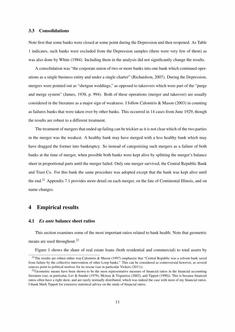
3.3 Consolidations

Note first that some banks were closed at some point during the Depression and then reopened. As Table

1 indicates, such banks were excluded from the Depression samples (there were very few of them) as

was also done by White (1984). Including them in the analysis did not significantly change the results.

A consolidation was “the corporate union of two or more banks into one bank which continued oper-

ations as a single business entity and under a single charter” (Richardson, 2007). During the Depression,

mergers were pointed out as “shotgun weddings,” as opposed to takeovers which were part of the “purge

and merge system” (James, 1938, p. 994). Both of these operations (merger and takeover) are usually

considered in the literature as a major sign of weakness. I follow Calomiris & Mason (2003) in counting

as failures banks that were taken over by other banks. This occurred in 14 cases from June 1929, though

the results are robust to a different treatment.

The treatment of mergers that ended up failing can be trickier as it is not clear which of the two parties

in the merger was the weakest. A healthy bank may have merged with a less healthy bank which may

have dragged the former into bankruptcy. So instead of categorizing such mergers as a failure of both

banks at the time of merger, when possible both banks were kept alive by splitting the merger’s balance

sheet in proportional parts until the merger failed. Only one merger survived, the Central Republic Bank

and Trust Co. For this bank the same procedure was adopted except that the bank was kept alive until

the end.21 Appendix 7.1 provides more detail on each merger, on the fate of Continental Illinois, and on

name changes.

4 Empirical results

4.1 Ex ante balance sheet ratios

This section examines some of the most important ratios related to bank health. Note that geometric

means are used throughout.22

Figure 1 shows the share of real estate loans (both residential and commercial) to total assets by21The results are robust either way.Calomiris & Mason (1997) emphasize that “Central Republic was a solvent bank saved

from failure by the collective intervention of other Loop banks.” This can be considered as controversial however, as severalsources point to political motives for its rescue (see in particular Vickers (2011)).

22Geometric means have been shown to be the most representative measure of financial ratios in the financial accountingliterature (see, in particular, Lev & Sunder (1979), Mcleay & Trigueiros (2002), and Tippett (1990)). This is because financialratios often have a right skew, and are rarely normally distributed, which was indeed the case with most of my financial ratios.I thank Mark Tippett for extensive statistical advice on the study of financial ratios.

11

.05

.1.1

5.2

.25

MO

RTG

AGES

_TA

1922h1 1924h1 1926h1 1928h1 1930h1 1932h1 1934h1halfyearly

Survivors June 1931 FailuresJune 1932 Failures June 1933 Failuresstandard error

Figure 1: Real estate loans to total assets (all categories)

Source: Statements.

cohort from 1923 onwards.23 In the pre-Depression era, survivors often had the lowest mortgage share

during most of the 1920s, followed closely by June 1933 failures.24 June 1932 failures had a sub-

stantially higher share, and the June 1931 failures share was even higher. Interestingly, some form of

divergence between June 1932 failures and survivors from around 1926 onwards is also noticeable, and

this difference becomes significantly larger starting in June 1928. This is evidence that the banks which

failed earlier were those that had invested more in real estate loans as early as 1923. In other words,

the share of mortgages at least partly explains not only the event of failure but also its timing.25 The

question is of course to what extent this was the case, and the econometric analysis provided below will

seek to give an answer.

The rise in the share of real estate loans after June 1929 is not surprising as most banks suffered a

large fall in total assets (see Figure 14 in Appendix 7.5). It will be seen later on that other kinds of assets

however declined as a share of total assets during the Depression, indicating that real estate loans were

more difficult to liquidate.23There is no decomposition of real estate loans on the books of Chicago state banks.24Note that June 1933 failures may have failed for reasons other than pure market discipline, as many were closed during

the national bank holiday in March 1933.25When examining these graphs, it will often appear that a large gap between any cohort and survivors signifies that the

variable is a good predictor of failure. A gap between failing cohorts themselves means that it is a good predictor of time offailure.

12

Regarding the size effect, it is interesting to note that four of the five largest state banks in Chicago

were survivors, and each of these four banks had a particularly low ratio of real estate loans to total

assets, even compared to the survivors average: in June 1929 Continental Illinois had .7 percent, Central

Trust Company of Illinois around 2 percent, Harris Trust and Savings .05 percent, and the Northern

Trust Company .7 percent.26 The fifth largest bank was part of the latest failure cohort, and had a larger

share invested in real estate (around 11 percent), which is representative of this cohort’s average at the

time.27

Although no other balance sheet item is as clearly graphically ordered as mortgage holdings (see

Figure 2 in this section, Figures 5, 7, 8, and 9 in Section 5.2, and Figures 10, 11, 12 and 13 in Appendix

7.2), it is necessary to test the precise importance of each variable econometrically. A simple way to

do so is to introduce an ordered logistic model, which for this study presents several advantages over

other estimation procedures. While in binary logistic models the outcome variable can only take one of

two values (“survivor” or “failure”), ordered logistic regression allows the outcome variable to include

several categories of failure, as well as the survivor one. And while a discrete-time hazard framework

necessarily takes into account within (ie. post-1929) Depression variables, ordered logistic models

allow one to focus exclusively on the impact of pre-Depression variables on the outcome.28 This matters

because external shocks may affect bank variables during the Depression, whereas ex ante variables

are more likely to reflect banks’ pre-Depression portfolio decisions, which are the subject of this study.

Nevertheless I report discrete-time hazard estimations in Appendix 7.3 for reference.

The dependent variable in the ordered logit model is thus an ordinal variable ( f ailure type) in which

each category represents a bank’s failure type. The categories are ordered so that the first category is

June 1931 failure (1), the second category is June 1932 failure (2), the third category is June 1933 failure

(3), and the last category is Survivor (4). Formally, I estimate a probabilistic model of bank failure such

that26See also Appendix 7.5 on bank size.27One may also wonder how a non-increasing share of real estate to total assets may have substantially weakened banks.

Appendix 7.6 deals with mortgage growth rates.28A discrete-time hazard model necessarily includes time-varying covariates up until the time of failure or censoring, which

in this dataset occurred mainly during, not before, the Depression. Although it is in theory possible to test the significance ofpre-Depression variables by adding interactions with time dummies, it is not possible to do so with this dataset as the hazardrate is very often zero prior to 1929. A hazard rate of zero means that time dummies will perfectly predict failure, which leadsto such dummies being automatically omitted from the model.

13

Table 3: Variable definitions

Variable Description

failure type ordinal dependent variable (1: June 1931 failure; 2: June 1932failure; 3: June 1933 failure; 4: Survivor)

size log (total assets)capital capital÷ total assetsreserve dep (cash balances + due from other banks)÷

(demand deposits + time deposits + due to other banks)gvtbds government bonds÷ total assetssecloans loans on security collateral÷ total assetsmortgages real estate loans (all categories)÷ total assetsother re other real estate÷ total assetsothloans other loans÷ total assetsbankhouse banking house÷ total assetsrearngs retained earnings÷ total capitalage dummy 1 = existed in May 1920;

0 = did not exist in May 1920

Notes: All variables except for size and age have been multiplied by 100 to ease interpre-tation of the odds ratios. The variable mortgages contains both residential and commercialmortgages as no decomposition was available on the original bank statements.

f ailure type = a +b1size+b2capital +b3reserve dep+b4gvtbds+b5secloans

+b6mortgages+b7other re+b8othloans+b9bankhouse

+b10rearngs+b11age+ e

(1)

where size is a value of bank size, capital is the capital ratio, reserve dep is the reserve-deposit ratio,

gvtbds is the share of U.S. government bonds, secloans represents loans on security collateral (short-

term loans backed by stock-market securities), mortgages is the share of real estate loans, other re is the

share of repossessed real estate after foreclosure, othloans is the share of other loans, bankhouse is the

share banking house, furniture and fixtures (bank expenses), rearngs is retained earnings to net worth

(a common measure of bank profitability),29 and age is a dummy variable equal to 1 if a bank already

existed in May 1920 and zero otherwise. The precise description of each variable is given in Table 3.

Table 4 presents the results for this model, in odds ratios. Each column represents a separate regres-

sion in which predictors are restricted to one particular year. For instance, the 1923 column helps find

out which 1923 variables best predict failure during the Depression.

Clearly, many ratios predict failure quite well throughout the pre-Depression period. In particular,29On 1929 financial statements retained earnings appear in the form of “undivided profits” or “the volume of recognized

accumulated profits which have not yet been paid out in dividends.” See Rodkey (1944, p. 108) and Van Hoose (2010, p. 12).

14

Table 4: Ordered logistic model of bank failure (odds ratios), 1923-1929 (dependent variable:failure type)

Dec1923

Dec1924

Jun 1925 Jun 1926 Jun 1927 Jun 1928 Dec1928

Jun 1929

size 1.620 1.421 1.207 1.708** 1.568 1.206 1.120 1.196(.56) (.43) (.29) (.49) (.46) (.31) (.28) (.27)

capital 1.027 .978 1.059 1.026 1.051 1.057 1.056 1.020(.06) (.04) (.04) (.04) (.04) (.04) (.04) (.04)

reserve dep 1.036 1.037 1.059 .988 .935 .965 .970 1.007(.05) (.04) (.04) (.03) (.04) (.04) (.02) (.02)

gvtbds 1.070* 1.044 1.070* 1.046 1.048 1.070 1.061 1.141**(.04) (.04) (.04) (.05) (.05) (.06) (.05) (.06)

secloans .987 1.020 1.025 .999 1.035 1.030 1.044** 1.023(.03) (.03) (.03) (.02) (.02) (.02) (.02) (.02)

mortgages .937** .928** .951* .919*** .940** .940** .930** .927***(.03) (.03) (.03) (.03) (.03) (.03) (.03) (.03)

other re .985 1.037 .937 .560** .477* .670 .568 .776(.12) (.09) (.12) (.15) (.20) (.23) (.24) (.18)

othloans 1.012 .971 .969* .978 .951** .973 .938** 1.003(.02) (.02) (.02) (02) (.02) (.02) (.02) (.02)

bankhouse .961 1.000 .939 1.072 .992 .922 .940 1.003(.08) (.08) (.07) (.05) (.07) (.06) (.05) (.06)

rearngs .995 1.030 1.025 1.057** 1.068** 1.035 1.036 1.060**(.03) (.03) (.03) (.03) (.03) (.02) (.03) (.03)

age .828 1.103 1.334 1.294 1.664 2.189* 3.249** (1.290)(.49) (.55) (.64) (.64) (.80) (1.00) (1.55) (.55)

n 86 102 103 111 112 122 116 128Prob > chi2 .006 .000 .000 .000 .000 .000 .000 .000Likelihood -98.78 -109.87 -111.91 -119.98 -116.85 -135.62 -125.21 -140.32

Notes: *** significant at a = 0.01, ** significant at a = 0.05, * significant at a = 0.10. The dependent variable(failure type) is an ordinal one, ordered in the following way: 1. June 1931 failure; 2. June 1932 failure; 3. June 1933failure; 4. Survivor. Each column represents a separate model run with variables taken each year before the start ofthe Depression. The table shows odds ratios, with standard errors based on the original coefficients in parentheses.An odds ratio above one increases the likelihood of survival, whereas an odds ratio below one decreases it. Eachvariable except for size and age has been multiplied by 100 so that a one unit increase can be interpreted as a onepercentage increase in the ratio. Source: Statements.

government bonds, other loans and especially retained earnings to net worth significantly each reduce

the likelihood of failure. The relative importance of the latter is also illustrated in Figure 2, which is

quite reminiscent of that of real estate loans, and is interesting in that the last failing cohort behaves

quite differently from survivors after 1926.

Of greater interest is the role of the real estate loan share. This variable stands out as the most

significant one overall. Already in December 1923, for a one percent increase in the proportion of

mortgages to total assets, the odds of surviving versus failing (all failure categories combined) were

.94 times lower, holding other variables constant in the model.30 This coefficient retains its significant30Recall that all ratio variables were multiplied by 100. This makes interpretation of the odds ratios more practical, as a

one-unit increase in the explanatory variable can now be interpreted as a “one percent” increase in the original proportion. Anodds ratio above one increases the likelihood of survival, whereas an odds ratio below one decreases it.

15

0.0

5.1

.15

REA

RN

GS_

TC



Figure 2: Retained earnings to net worth

Source: Statements.

predictive power compared to all other variables throughout the 1920s, up until the eve of the Depression

(June 1929). No other variables is as consistently significant as the real estate loan share throughout the

period.31

31The relative insignificance of other re will be explained in more detail in Section 5.2.

16

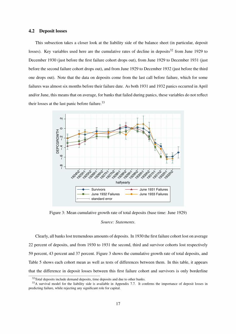
4.2 Deposit losses

This subsection takes a closer look at the liability side of the balance sheet (in particular, deposit

losses). Key variables used here are the cumulative rates of decline in deposits32 from June 1929 to

December 1930 (just before the first failure cohort drops out), from June 1929 to December 1931 (just

before the second failure cohort drops out), and from June 1929 to December 1932 (just before the third

one drops out). Note that the data on deposits come from the last call before failure, which for some

failures was almost six months before their failure date. As both 1931 and 1932 panics occurred in April

and/or June, this means that on average, for banks that failed during panics, these variables do not reflect

their losses at the last panic before failure.33

−.8

−.6

−.4

−.2

0.2

DEPC

GRO

WTH

1924

h2

1925

h1

1925

h2

1926

h1

1926

h2

1927

h1

1927

h2

1928

h1

1928

h2

1929

h1

1929

h2

1930

h1

1930

h2

1931

h1

1931

h2

1932

h1

1932

h2

halfyearly


Figure 3: Mean cumulative growth rate of total deposits (base time: June 1929)

Source: Statements.

Clearly, all banks lost tremendous amounts of deposits. In 1930 the first failure cohort lost on average

22 percent of deposits, and from 1930 to 1931 the second, third and survivor cohorts lost respectively

59 percent, 43 percent and 37 percent. Figure 3 shows the cumulative growth rate of total deposits, and

Table 5 shows each cohort mean as well as tests of differences between them. In this table, it appears

that the difference in deposit losses between this first failure cohort and survivors is only borderline32Total deposits include demand deposits, time deposits and due to other banks.33A survival model for the liability side is available in Appendix 7.7. It confirms the importance of deposit losses in

predicting failure, while rejecting any significant role for capital.

17

Table 5: Tests of differences between mean deposit growth rates

Survivors June 1931 June 1932 June 1933(1) (2) (3) (1) (1) (2) (1) (2) (3)

Mean -.08 -.37 -.59 -.22 -.17 -.59 -.00 -.43 -.63(.07) (.06) (.08) (.04) (.03) (.03) (.13) (.10) (.09)

June 1931(t-stat)

1.806*

June 1932(t-stat)

1.298 3.380*** -.995

June 1933(t-stat)

-.527 .472 .366 -1.606 -1.288 -1.550

Observations 35 46 36 14

Notes: * significant at a = 0.01, ** significant at a = 0.05, *** significant at a = 0.10.(1) June 1929 - Dec 1930 cumulative deposit losses;(2) June 1929 - Dec 1931 cumulative deposit losses;(3) June 1929 - Dec 1932 cumulative deposit losses.First row gives the mean deposit growth rates (standard errors in parentheses). Next rows give t-statistics of differ-ences between two means. Source: Statements.

significant, and is not significant when comparing to other failure cohorts. On the other hand, the

magnitude of the second failure cohort’s withdrawals significantly differs from survivors’.34 Yet even

in this case deposit losses were very large for survivors (around 37 percent compared to 59 percent for

June 1932 failures). By June 1932, survivors themselves had lost an outstanding 60 percent of total

deposits.35 Together these results suggest that while mortgages remain essential to explain Chicago

bank failures, the role of mass deposit withdrawals cannot be disregarded.

Now, the causes of these large withdrawals in preceding non-panic windows are open to debate.

Tentative answers may be found in the literature on bank runs. According to Diamond & Dybvig (1983),

bank runs are undesirable equilibria in which borrowers observe random shocks (sunspots) and withdraw

their deposits, thus causing even “healthy” banks to fail. Others, such as Calomiris & Gorton (1991)

and Calomiris & Kahn (1991), have stressed the role of signal extraction in the context of asymmetric

information between depositors and bank managers. In this view, depositors observe a specific shock to

banks’ assets, but do not know which banks have been most hit. They therefore run on all banks, which

causes only the weaker banks to fail. Bank runs thus act as a form of monitoring: unable to costlessly

value banks’ assets, borrowers use runs to reveal the unhealthy banks.

In Chicago, depositors in theory could know which banks had the highest amounts of mortgages34Note that these figures differ slightly from Calomiris & Mason (1997)’s as their sample included national banks as well.

Their survivor category also includes my June 1933 Failures cohort.35Note that some central-reserve city banks in the Loop, most of which ended up surviving, benefited from an inflow of

deposits in the summer 1931 crisis as outlying banks closed and some of the money was redeposited in the Loop banks (see,in particular, Mitchener & Richardson (2013) and U.S. Congress (1934, part 2, p. 1062)). Despite such inflows their totalcumulative deposit losses were very large, as Figure 3 suggests.

18

thanks to official publications of balance sheet summaries every six months. This suggests that the initial

cause of withdrawals is indeed still to be found. Nevertheless, the fact that differences in withdrawals

did widen to some extent after June 1931 may be explained by a learning effect on the part of creditors.

As creditors witnessed withdrawals and the failure of banks with the largest amounts of mortgages in the

first episode, they withdrew more from banks with larger amounts of such assets subsequently. However

this information effect cannot entirely explain, for instance, why survivors themselves ended up losing

nearly 60 percent of their deposits.

So why did mortgages matter so much in practice, given large deposit withdrawals? Did banks fail

simply because they had a particularly large share of illiquid mortgages, or because of the particularly

low quality (in terms of underlying values) of these mortgages? It is to this question that I now turn.

5 The role of mortgages

The aim of this section is to explain the importance of mortgages as a determinant of bank failure.

It will start by giving some background information on the Chicago building boom of the 1920s, which

explains the large share of mortgages on banks’ portfolios. It will then move on to an exposition of the

reasons why mortgages’ illiquidity came to be more problematic than their low quality.

5.1 Unit banking and the Chicago building boom

Already in August 1929, an article published in the Chicago Tribune entitled “Claim Illinois is Over-

loaded with Banks” expressed concern that too many banks were in operation for too small a number

of people (Chicago Tribune, n.d.). And, according to James, “[these banks’] soundness was intimately

related to the building boom” (James, 1938, p. 953).

The boom itself was the result of circumstances created by World War I. On the one hand, a near

wartime embargo on building material and labour created a housing shortage which realtors were eager

to compensate for after the war (U.S. Congress, 1921). On the other hand, the war led to a substantial

boom in agricultural goods and land, which quickly gave way to a deep recession in farming areas when

the war came to an end. As a flourishing business centre lying next to the vast but weakened agricultural

lands of the Midwest, Chicago profited from this situation perhaps more than any other city in the U.S.

The excitement that the progress in economic activity and the near-constant arrival of new dwellers

in search of higher wages brought to the city led to an extremely fast development of credit (James, 1938,

p. 939). Eichengreen & Mitchener (2003) stress the interaction between the structure of the financial

19

sector and the business boom. While the rapid growth of installment credit first started with nonbank in-

stitutions,36 very quickly many sorts of financial institutions ended up competing for consumers’ credit.

One of the consequences of this credit expansion in Chicago was the boom in construction activity.37

The Chicago real estate boom was excessive in the sense that it reflected predictions of population

increase that went far beyond the actual increase. Hoyt shows how as Chicago’s population started

growing at an unusually rapid rate investors imagined that a “new era” was born and that Chicago would

grow to 18 million by 1974 (Hoyt, 1933, p. 403).38 While from 1918 to 1926 the population of Chicago

increased by 35 percent, the number of lots subdivided in the Chicago Metropolitan Region increased by

3,000 percent (ibid., p. 237).39 But a population slowdown occurred in 1928, just before the start of the

Depression. Figure 4 shows that the Chicago building boom reached a peak in 1925 and then receded

abruptly.

-

2,000

4,000

6,000

8,000

10,000

12,000

14,000

16,000

18,000

20,000

1915

1916

1917

1918

1919

1920

1921

1922

1923

1924

1925

1926

1927

1928

1929

1930

1931

1932

1933

Figure 4: Annual amount of new buildings in Chicago

Source: Hoyt (1933, p.475).

The role that small state banks played in allowing this building boom to occur was a determinant

one. In December 1929, state banks made up 95.5 percent of all banks in the city (University of Illinois

Bulletin, 1929). There were few national banks; however these banks were large. Indeed at the time they36For example, in 1919 General Motors established the General Motors Acceptance Corporation (GMAC) to finance the

development of its mass market in motor vehicles.37White (2009) studies the question for the country as a whole but does not disaggregate into the various regions and cities

of the U.S.. For journalistic accounts see Allen (1931) and Sakolski (1966).38Hoyt humorously depicts “distinguished scholars”’ assessments of the situation, which were often quite surprising (Hoyt,

1933, p. 388).39In 1928, Ernest Fisher, associate professor of real estate at the University of Michigan, studied real estate subdividing

activity and found that “periods of intense subdividing activity almost always force the ratio of lots to population considerablyabove the typical” (Fisher, 1928, p. 3). His explanation was that “the only basis for decision is the position of the market at thetime the manufacturer [makes] his plans,” which leads to procyclicality.

20

reported close to 40 percent of the aggregate resources of all banks (ibid.). The largest of these national

banks, First National, rivaled in size the largest bank in Chicago (Continental Illinois, which was state-

chartered). As a contemporary made clear, “by the summer of 1929, then, the Continental Illinois and

the First National towered over the Chicago money market like giants” (James, 1938, p. 952).40 Yet a

huge number of small unit banks swarmed around the city, most of them state-chartered. As James put

it “around these great banks of the Loop, there nestled, however, some 300 outlying commercial banks,

each of which appeared microscopic with the Continental or the First although, in the aggregate, they

handled a considerable proportion of the city’s business.”

These small banks were usually unable to branch, due to state banking laws in Illinois which pre-

vented them from doing so. Such restrictions likely created incentives for unit banks to make the most

of local profit-making opportunities, such as real estate lending. Had they been allowed to branch, they

would have likely been able to better diversify their assets and prepare for a sudden backlash (Carlson,

2001; Calomiris & Mason, 2003; Mitchener, 2005). See Appendix 7.4 for a more complete discussion

of the role of unit banking in the Chicago boom.

5.2 The impact of mortgage illiquidity

Despite the excessive proportions of the real estate boom, evidence suggests that the role of mort-

gages’ quality in causing banks’ failure was minor. Indeed, what really mattered was their inherent lack

of liquidity, for three reasons.

First, mortgages at the time only had a 50 percent loan-to-value ratio (LTV), which is particularly low

compared to today’s standards.41 This has been emphasized both by Field (2013) and White (2009).42

Given that land values in Chicago never fell by more than 50 percent until 1933, and that most Chicago

banks failed before then (see Table 2), they could not have made any substantial losses on these loans,

even after foreclosure. The fall in land values is documented by Hoyt (1933, p. 399), who shows that

Chicago land values fell by 5 percent in 1929, 20 percent in 1930, 38 percent in 1931, 50 percent in40Indeed, together they were responsible “for about half of the banking business transacted in the city” (ibid.).41In Chicago specifically, a survey conducted in 1925 indicates that the average LTV on residential properties varied from

41.3 percent to 50.5 percent. First mortgages on apartments encumbered by a second mortgage (which constituted the majorityof cases for apartments) had an average LTV of 54.7 percent. In other cases (especially when apartments were not encumberedby a second mortgage) LTVs could go up to 59.9 percent. Interest rates on average reached around 6 percent (Bayless &Bodfish, 1928).

42This low average LTV is in fact one of the main arguments put forward by Field and by White against any possiblecausation link between mortgage holdings and bank failures. As this section will go on to suggest, low LTVs partly explainwhy the quality of mortgages did not matter, but do not preclude mortgages’ lack of liquidity from having a detrimental impacton bank survival.

21

Table 6: Percentage of banks by cohort falling into one of the three cate-gories of cumulative value decline from 1926 to 1931 (lowest to highest)

Fall in land val-ues

June 1931Failures

June 1932Failures

June 1933Failures

Survivors

0 36.96 28.57 30.77 45.451 58.70 68.57 38.46 48.482 4.35 2.86 30.77 6.06

Total 100 100 100 100

Source: Hoyt (1933, pp. 259, 267) and Statements.

1932 and 60 percent in 1933.43

Further, I use Hoyt (1933, pp. 259, 267)’s sectoral data on land values to test the hypothesis that

differences in land values were uncorrelated with bank failure rates. Although Hoyt’s land value variable

is categorical, his maps are detailed enough to allow efficient matching with my balance sheet data,

using banks’ contemporary addresses in Chicago. I thus generated a new categorical variable, valuefall,

which includes three categories of cumulative fall in residential land values per front foot from 1926 to

1931 (from lowest to highest) in each bank’s sector.44 As mentioned earlier, banks were numerous and

spread out around the city, which makes it reasonable to assume that they catered mainly to their own

neighbourhoods,45 so that land values in their own sector would likely have had the highest impact

on their health. Although 1931 is the latest available year, it was chosen by Hoyt to illustrate the

geographical pattern of falls in land values in the city as this was when the first sharp decline in values

occurred (ibid., p. 266). It is reasonable to assume that subsequent falls in land values followed the

initial geographical pattern in terms of differences in intensity.46

Table 6 shows the percent of banks in each cohort by category of value decline. There are few

differences within the three failing cohorts, so that falls in land values do not point to any possible

correlation between falls in land values between 1926 and 1931 and those cohorts’ timing of failure. In

addition, although survivors seem to have experienced less of a decline in values than all other cohorts

together, many survivors were very large banks from the Loop, where land values were more stable43These land values are mainly based on sales and real estate brokers’ opinions rather than assessments for tax purposes.

Note also that very few banks failed after March 1933, but that one cannot know whether most of the “1933” decline occurredbefore the national bank holiday in March 1933 or after. On p. 172 Hoyt asserts that “the decline in the value of improvedproperties from 1928 to 1933 was 50 per cent,” not 60 per cent (Hoyt, 1933).

44This variable was generated using the two maps shown in Figures 42 and 47 in Hoyt (1933, pp. 259, 267). For these mapshe used sales data from Olcott’s Land Values Blue Book of Chicago and land assessment data from Jacob (1931). These mapsare divided into grids, and a bank’s sector is one of the 219 squares on each grid. Each square’s size is about 2.5 squaredkilometers.

45This is confirmed by James (1938).46Indeed, while it is likely that a particular section of Chicago saw further declines in land values after 1931, the assumption

that the geographical pattern of differences in intensity between regions remained stable seems reasonable.

22

throughout the period. Controlling for size may therefore be important when assessing the role of land

value falls. More generally, should there be any relationship between land values and bank failures, it

may not be a directly causal one: sectors experiencing a larger fall in land values may also be sectors

in which banks simply made larger amounts of mortgages in the 1920s, which may lead land values to

be related to bank failures only indirectly and not through loan losses. Controlling for other financial

ratios may therefore also be important. Table 7 reports estimates of the same ordered logistic model as

before, only with 1929 balance sheet variables on the right-hand side and the added valuefall variable.

This variable remains insignificant regardless of whether mortgages are included or not.

Interestingly, a simple t-test reveals that deposit losses among all cohorts are uncorrelated with falls

in land values. This holds for deposit losses up to December 1930 (Prob > F = 0.701) as well as for

deposit losses up to December 1931 (Prob > F = 0.080).

The fact that banks’ losses did not have a large impact on bank failure can also be seen in the low

predictive power of capital ratios throughout the period (see Table 4). As Figure 5 suggests, June 1931

failures had the highest ratio of capital to total assets through most of the 1920s, despite being the first

cohort to fail.47

Finally, although mortgages’ contract maturity was usually only three to five years, their de facto

maturity in the 1920s was much longer. Precisely because these loans were relatively short-term (and

perhaps for other reasons), it was customary for banks to renew them. As Saulnier made clear in his 1956

study of 1920s mortgage lending in the U.S., “the much lauded feature of full repayment by maturity has

been won at the price of extended maturities” (see Morton (1956, p. 8) and Chapman & Willis (1934,

p. 602)). This created entrenched renewal expectations on the part of borrowers, who after three or five

years, having only made the initial down payments and interest payments – loans were unamortized –,

expected to be given another three to five years to make the final “balloon” payment. This is illustrated

in the following quote:“Another thorn was the uncertainty and recurring crises in the credit arrangements inher-

ent in the then prevalent practice of buying a home with a first mortgage written for one tofive years, without any provision for paying back the principal of the loan during that time.This latter device was a fair weather system, and, as is the case with most such systems,nobody suspected that there was anything wrong with it until the weather changed.

47There are unfortunately no good statistics on the rate of foreclosure for commercial banks in Chicago. Most of the numbersare provided by Hoyt (1933, p. 269-270), and they concern the total amount of foreclosures: “Foreclosures were mountingrapidly, the number increasing from 5,818 in 1930 to 10,075 in 1931 (...), [and] reached a new peak in 1932, rising to (...)15,201.” It is thus not possible to describe banks’ precise losses in real estate. In any case, as will be shown later, foreclosuresonly mattered for banks insofar as it took more than eighteen months to foreclose in Illinois, which greatly impeded banks’liquidity during crises.

23

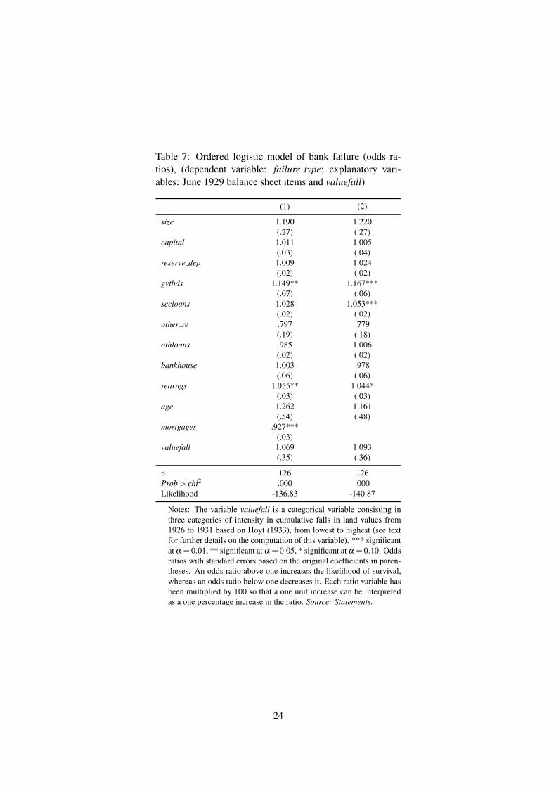
Table 7: Ordered logistic model of bank failure (odds ra-tios), (dependent variable: failure type; explanatory vari-ables: June 1929 balance sheet items and valuefall)

(1) (2)

size 1.190 1.220(.27) (.27)

capital 1.011 1.005(.03) (.04)

reserve dep 1.009 1.024(.02) (.02)

gvtbds 1.149** 1.167***(.07) (.06)

secloans 1.028 1.053***(.02) (.02)

other re .797 .779(.19) (.18)

othloans .985 1.006(.02) (.02)

bankhouse 1.003 .978(.06) (.06)

rearngs 1.055** 1.044*(.03) (.03)

age 1.262 1.161(.54) (.48)

mortgages .927***(.03)

valuefall 1.069 1.093(.35) (.36)

n 126 126Prob > chi2 .000 .000Likelihood -136.83 -140.87

Notes: The variable valuefall is a categorical variable consisting inthree categories of intensity in cumulative falls in land values from1926 to 1931 based on Hoyt (1933), from lowest to highest (see textfor further details on the computation of this variable). *** significantat a = 0.01, ** significant at a = 0.05, * significant at a = 0.10. Oddsratios with standard errors based on the original coefficients in paren-theses. An odds ratio above one increases the likelihood of survival,whereas an odds ratio below one decreases it. Each ratio variable hasbeen multiplied by 100 so that a one unit increase can be interpretedas a one percentage increase in the ratio. Source: Statements.

24

.1.2

.3.4

CAP

_TA



Figure 5: Capital to total assets

Source: Statements.

What usually happened was that the average family went along, budgeting for the inter-est payments on the mortgage, subconsciously regarding the mortgage itself as written foran indefinite period, as if the lender were never going to want his money back (...). This im-pression was strengthened by the fact that lenders most frequently did renew the mortgageover and over again when money was plentiful” (Federal Home Loan Bank Board, 1952,pp. 2-5).

As a consequence, while most loans were made in the boom years of 1925 to 1927 (see Figure 6),

those maturing between 1929 and 1930 were likely renewed and would not actually come due before

1932-35.48 In addition, loans maturing for the first time during the Depression would come up for

(expected) renewal, with banks under liquidity pressure pressing unprepared borrowers to pay back their48This is confirmed by Morton (1956), who derived figures on contract maturity from a National Bureau of Economic

Research survey of urban mortgage lending, whose absolute precision may be taken with care. The survey was made in 1947on a sample of 170 surviving commercial banks of all sizes, “representing about one-third of the commercial banks totalnonfarm mortgage portfolio as of mid-1945” (ibid., p. 71). The precise average contract length for loans made in 1926 was 3.6years (for commercial banks), and 3.1, 2.5 and 3.2 years for loans made in 1925, 1927 and 1928 respectively (ibid., p. 174).For 1927 loans, maturity would be reached around mid-1929, and for 1928 loans around mid-1931. In 1925 the amount ofnew mortgages in Cook County was slightly lower than in 1927, but taking this year into account would still mean that a largeportion of mortgages were expected to be refinanced in early 1929 (the average contract length for 1925 loans was 3.1 years).Morton points out that even for mortgages made in the 1925-29 period, the realized maturity was 8.8 years (ibid., p. 119).

25

0

500

1000

1500

2000

-

200,000,000

400,000,000

600,000,000

800,000,000

1,000,000,000

1,200,000,000

1920 1921 1922 1923 1924 1925 1926 1927 1928 1929 1930 1931

Figure 6: New mortgages and trust deeds, Cook County, Illinois ($)

Note: the source does not specify whether new mortgages include renewed mortgages. Source: Hoyt(1933, p.475).

loans.49 In such cases foreclosure would not entail any loss (due to the 50 percent LTV),50 but it would

create a clear liquidity issue as the foreclosure process in Illinois lasted more than eighteen months on

average (Child, 1925; Gries & Ford, 1932; Hoppe, 1926; Johnson, 1923).51

Mortgages’ sheer lack of liquidity thus posed a tremendous challenge to banks. In the interwar period

mortgages could neither be sold in the secondary market nor rediscounted at the Federal Reserve.52

49As the vice-president of the banking department of the First National Trust and Savings Bank in Chicago put it: “I haveheard a lot of talk about foreclosures and that the banks are calling loans and insisting upon repayment and that the borrowersare unable to refund elsewhere, and they are doing this because they are trying to keep their assets liquid” (U.S. Congress,1932, part 2, p. 269). This is confirmed in Federal Home Loan Bank Board (1934), which mentions “the dangers attendant onthe mortgagee’s refusal to renew,” and in Federal Home Loan Bank Board (1952), which reports: “The time of stress came in1929-30; the short-term mortgage came to maturity against a situation of tight credit and, in many cases, of no credit (...). Alltoo often the lender (...) did not want to renew the loan to the home-owner no matter how high the premium or rate of interest.”Note, in addition, that second mortgage financing made prompt repayment even less likely – see Postel-Vinay (2014).

50After foreclosure either the property could be auctioned off to external buyers or, if there were no buyers, the property wasrepossessed by the bank at an appraisal price. Such repossessed property then sat on the bank’s books as non-performing assets(called “other real estate”) until they could be sold again later. Arguably, the foreclosure price could potentially be lower thanthe current “market” price. Nevertheless, it is important to note that in Depression Chicago transactions were few, foreclosureswidespread (Hoyt, 1933, p. 266-272), and sales prices were probably themselves affected by foreclosures in surrounding areas(this theoretical point is made by Campbell et al. (2011); see also Genesove & Mayer (2001)). This suggests that gaps betweenforeclosure and sales prices may not have been very large. Further comments on the meaning and significance of other realestate in the dataset under study can be found at the end of this sub-section.

51This was particularly emphasized by Gries & Ford (1932, p. 39): “One of the greatest hindrances to the availability ofmortgage money in some states is the right of redemption from sale under foreclosure. During the period of redemption,foreclosed property is rendered practically unmarketable, may suffer serious damage or depreciation, and presents in a highdegree a type of frozen asset.” See also Anderson (1927), Hopper (1927), Stalker (1925), and Postel-Vinay (2014).

52Note that in early 1932 the Reconstruction Finance Corporation proposed to lend against “ineligible” collateral, whichcould include high quality real estate loans. Nevertheless loans against such assets remained proportionately small as the RFCpreferred loans with maturities of less than six months (Calomiris et al., 2013) and refused to lend against real estate loans’book value, likely taking into account their uncertain quality paramount to their long maturity (Wigmore, 1995, p.324). Ingeneral the RFC remained very cautious and mainly lent against high-quality and liquid collateral, until 1933 when it switchedto preferred stock purchases in financial institutions (Calomiris & Mason, 2004; Calomiris et al., 2013; James, 1938; Mason,2001). In addition, around the same time the Banking Act of 1932 also allowed the Federal Reserve to widen its acceptedcollateral for rediscounts. According to Friedman & Schwartz (1963, p. 45), however, such powers were used only to a very

26

Figure 1 showed how real estate loans increased as a share of total assets for all banks during the

Depression, at the same time as assets as a whole were diminishing.53 Other types of loans, on the other

hand, were promptly liquidated in this period. Figure 7 shows the falling share of loans on collateral

security owned by banks,54 while Figure 8 shows a similar decline in other loans as a share of total

assets. Compared to other assets, therefore, mortgages were notoriously difficult to liquidate.55 As all

banks engaged in fire sales they became the main constraint on their liquidation process.

As a final note, the variable “other real estate” deserves special attention. Other real estate is an

asset consisting of property repossessed by banks after real estate foreclosures and before it can be

resold. One might question the importance of this variable in explaining bank failures given the very low

percentages shown in Figure 9, which never go much beyond 3 percent, and given the low significance of

this variable in the ordered logit model. This can be explained, first, by the fact that mortgages’ impact

on bank failure could have been strong without any foreclosures taking place. When foreclosures did

occur, it is precisely their very lengthy process that would have created liquidity problems for banks.

Each cohort’s last data point represents its status at the last call before failure, and each call occurred

only every six months. This means that if many banks failed between April and June, which was the

case for the first two failing cohorts, it is likely that much of their repossessed property would not have

been recorded by December before this date. Thus, the lengthy foreclosure process increases the odds

that many of the effects of foreclosure are not visible on this graph (Child, 1925; Hoppe, 1926; Johnson,

1923).56

limited extent, perhaps for the same reason. See also Mason (2001) and Wicker (1996, p.85).53For a graph of total assets see Figure 14 in Appendix 7.5.54Security loans were mainly call loans, that is, loans repayable at the option of the lender within twenty-four hours’ notice.

Funds were lent in this way to individuals who used them to carry securities, for example when dealing with them on margin.The securities themselves were used as collateral for these loans, with the understanding that they were likely to be withdrawnat any time. According to Bogen & Willis (1929, p. 245), “depositors can, and sometimes do, determine the calling of loans bythe activity of their own demands.” Other loans were short-term commercial loans, often sought by companies for the seasonalexpansion of their inventories. In such cases “the customer of the commercial bank is expected to pay off or “clean up” hisobligations to it at certain intervals” (ibid., p. 11). Both types of loans were eligible for rediscount at the Federal Reserve Banksor could be sold in the open market, while mortgages in general were not (Bogen & Willis, 1929; U.S. Congress, 1927).

55Note, perhaps surprisingly, that cash is not a good predictor of failure. This suggests that cash ratios were relativelysimilar for all four cohorts, and that what really differentiated them were their mortgage holdings. Government bonds weremore important than cash, as can be seen in Table 4 and Figure 11 in Appendix 7.2.

56Further comments on the value of repossessed property after foreclosure are made earlier in this sub-section.

27

.1.2

.3.4

SECL

OAN

S_TA



Figure 7: Loans on collateral security to total assets

Source: Statements.

0.0

5.1

.15

.2.2

5O

THLO

ANS_

TA



Figure 8: Other loans to total assets

Source: Statements.

28

0.0

1.0

2.0

3.0

4O

THER

_RE_

TA



Figure 9: Other real estate to total assets

Source: Statements.

6 Conclusion

Looking into the long-term behaviour of Chicago banks in the 1920s yielded new insights into the causes

of their failure. I showed that banks’ long-term investments in illiquid assets (especially mortgages)

severely weakened their position when they came to face large withdrawals on their deposits. Though

restricted to Chicago, these results reassert the role that liquidity issues played in the Great Depression,

both on the liability and the asset sides of the balance sheet. More specifically, they suggest that a

solvent but ex ante less liquid bank is not necessarily healthy, and that liquidity risk management is

just as important as credit risk management when the occurrence of bank runs cannot be completely

excluded.

This paper also reassessed the role that mortgage investments played in the Great Depression via

the banking channel. Parallels with the recent crisis may be tentatively drawn, despite major differences

in mortgage contracts then and now. In both cases banks suffered tremendous liquidity shocks on the

uninsured liability side of their balance sheets, which, regardless of their origin, highlighted once again

the impact of maturity mismatches between long-term assets and short-term liabilities (Brunnermeier,

2008; Gorton & Metrick, 2012). Securitization can potentially increase the liquidity of mortgages by

making them more salable and by distributing different kinds of risks to different types of investors. But

29

in order to do so it has to be undertaken in the right way (see Postel-Vinay (2013)).

Central banks can in theory help during a liquidity crisis by following Bagehot’s rule and lending

on good (though not perfect) collateral. Although central banks’ role during crises is essential, it is

always difficult for it to gauge the precise quality (credit risk) of an asset – especially if the asset is a

long-term one, thereby creating more uncertainty about its long-term value (Goodhart, 2008, 2010). For

this reason, the Federal Reserve’s role in the recent crisis has been controversial: by actually lending

against such doubtful collateral as mortgage-backed securities it has once again raised the question as

to how a central bank can measure asset risk (Bordo & Landon-Lane, 2010; Schleifer & Vishny, 2011;

Gorton & Metrick, 2013; Stein, 2013).57

Because central bank help will likely never be entirely adequate, it is important for banks to attend to

the inherent liquidity of their portfolios. Of course, nowadays assets’ liquidity is increasingly intertwined

with their quality as markets are formed and disappear in terms of the perceived quality of such assets.

Nevertheless, some assets are inherently less liquid than others, and longer-term assets tend to be less

liquid either because they are paid back in a long time or because of the uncertainty attached to their

long maturity. Conversely, some assets are inherently more liquid than others, such as cash assets and

(usually) government bonds.

No bank will ever be perfectly hedged in terms of its maturity profile, but promoting liquidity in a

preventive regulatory framework, perhaps through countercyclical cash ratios may be a good start. In this

paper, cash did not matter in the sense that differences in mortgage holdings made a larger difference.

But it is possible to speculate that had banks holding more mortgages also held more cash, they would

not have run into such difficulty in the face of bank runs.58 Although Basel I and Basel II had a clear

focus on capital rather than liquidity, Basel III has started to introduce measures to regulate the latter

(Basel Committee on Banking Supervision, 2008). Yet it has mainly focused on so-called “liquidity

coverage ratios,” which may be inadequate as their vagueness could lead to new forms of risk-shifting.

Cash may be a simpler and more transparent way of assessing a bank’s liquidity. And, in turn, increased

liquidity in the system may reduce the risk of runs, as runs can partly be triggered by fears of banks’

illiquidity, not just by fears regarding their potential insolvency.59

57And by purchasing such securities outright, it clearly cut across the boundary between monetary and fiscal policy (Rein-hart, 2011).

58Note that government bonds mattered more than cash, as can be seen in Table 4 and Figure11 in Appendix 7.2.59See also Calomiris et al. (2012), Goodhart (2008, 2010) and Shin (2009). Note that Calomiris et al. (2012) also see cash

ratios as important buffers against credit risk.

30

References

F. L. Allen (1931). Only Yesterday: An Informal History of the Nineteen-Twenties. Harper and Brothers,New York.

F. H. Anderson (1927). ‘Essential and Practical Covenants of First and Second Mortgages’. Real EstateFinance 5.

Basel Committee on Banking Supervision (2008). Principles for Sound Liquidity Risk Management andSupervision. Bank of International Settlements.

A. C. Bayless & M. H. Bodfish (1928). ‘Costs and Encumbrance Ratios in a Highly Developed RealEstate Market’. The Journal of Land and Public Utility Economics 4(2).

Board of Governors of the Federal Reserve System (1937). Federal Reserve Bulletin. Federal ReserveSystem.

J. I. Bogen & H. P. Willis (1929). Investment Banking. Harper & Brothers, New York.

M. Bordo & J. Landon-Lane (2010). ‘The banking panics of the United States in the 1930s: somelessons for today’. Oxford Review of Economic Policy 26(3).

M. K. Brunnermeier (2008). ‘Deciphering the Liquidity Credit Crunch 2007-08’. NBER Working Paper14612.

C. W. Calomiris & G. Gorton (1991). ‘The Origins of Banking Panics: Models, Facts, and Bank Regu-lation’. In R. G. Hubbard (ed.), Financial Markets and Financial Crises. The University of ChicagoPress.

C. W. Calomiris, et al. (2012). ‘A Theory of Bank Liquidity Requirements’. Working Paper.

C. W. Calomiris & C. M. Kahn (1991). ‘The Role of Demandable Debt in Structuring Optimal BankingArrangements’. The American Economic Review 81(3).

C. W. Calomiris & J. R. Mason (1997). ‘Contagion and Bank Failures During the Great Depression: theJune 1932 Chicago Banking Panic’. American Economic Review 87(5).

C. W. Calomiris & J. R. Mason (2003). ‘Fundamentals, Panics, and Bank Distress During the Depres-sion’. American Economic Review 87(5).

C. W. Calomiris & J. R. Mason (2004). ‘How to Restructure Failed Banking Systems: Lessons fromthe United States in the 1930s and Japan in the 1990s’. In T. Ito & A. Krueger (eds.), Governance,Regulation, and Privatization in the Asia-Pacific Region, NBER East Asia Seminar on Economics,Volume 12. University of Chicago Press.

C. W. Calomiris, et al. (2013). ‘The Effects of Reconstruction Finance Corporation Assistance onMichigan’s Banks’ Survival in the 1930s’. Explorations in Economic History 50.

C. W. Calomiris & D. C. Wheelock (1995). ‘The Failures of Large Southern Banks During the GreatDepression’. Columbia University Working Paper .

G. Calvo (2013). ‘Puzzling Over the Anatomy of Crises’. Working Paper.

J. Y. Campbell, et al. (2011). ‘Forced Sales and House Prices’. American Economic Review 101.

31

M. Carlson (2001). ‘Are Branch Banks Better Survivors? Evidence from the Depression Era’. FederalReserve Board Working Paper 2001(51).

S. B. Carter, et al. (2006). Historical Statistics of the United States. Cambridge University Press,Cambridge.

J. M. Chapman & H. P. Willis (1934). The Banking Situation, American Post-War Problems and Devel-opments. Columbia University Press, New York.

Chicago Tribune (n.d.). Various issues. Chicago Tribune, Chicago, Ill.

S. R. Child (1925). ‘A Uniform Mortgage Law for All the States’. Real Estate Finance .

D. W. Diamond & P. H. Dybvig (1983). ‘Bank Runs, Deposit Insurance, and Liquidity’. Journal ofPolitical Economy 91(3).

B. Eichengreen & K. Mitchener (2003). ‘The Great Depression as Credit Boom Gone Wrong’. BISWorking Paper 137.

M. Esbitt (1986). ‘Bank Portfolios and Bank Failures During the Great Depression: Chicago’. Journalof Economic History 46(2).

Federal Home Loan Bank Board (1934). Federal Home Loan Bank Review. Federal Home Loan Banks.

Federal Home Loan Bank Board (1952). The Federal Home Loan Bank System, 1932-195. FederalHome Loan Banks, Washington, D. C.

A. J. Field (2013). ‘The Interwar Housing Cycle in the Light of 2001-2011: A Comparative HistoricalApproach’. NBER Working Paper 18796.

P. Fishback, et al. (2001). ‘The Origins of Modern Housing Finance: the Impact of Federal HousingPrograms During the Great Depression’. Working Paper.

P. Fishback, et al. (2009). ‘The Influence of the Home Owners Loan Corporation in Housing MarketsDuring the 1930s’. Working Paper.

P. Fishback, et al. (2013). Well Worth Saving: How the New Deal Safeguarded Home Ownership.University of Chicago Press., Chicago.

E. M. Fisher (1928). ‘Real Estate Subdividing Activity and Population Growth in Nine Urban Areas’.Michigan Business Studies 1(9).

M. Friedman & A. J. Schwartz (1963). A Monetary History of the United States, 1867-1960. PrincetonUniversity Press, Princeton.

C. M. Gambs (1977). ‘Bank Failures - An Historical Perspective’. Monthly Review Federal ReserveBank of Kansas City 62.

D. Genesove & C. Mayer (2001). ‘Loss Aversion and Seller Behavior: Evidence from the HousingMarket’. The Quarterly Journal of Economics 116(4).

C. A. Goodhart (2008). ‘Liquidity risk management’. Banque de France Financial Stability Review 11.

C. A. Goodhart (2010). ‘The changing role of central banks’. BIS Working Papers 326.

G. Gorton & A. Metrick (2012). ‘Securitized Banking and the Run on Repo’. Journal of FinancialEconomics 104:425.

32

G. Gorton & A. Metrick (2013). ‘The Federal Reserve and Panic Prevention: The Roles of FinancialRegulation and Lender of Last Resort’. Journal of Economic Perspectives 27(4).

J. M. Gries & J. Ford (1932). The Presidents Conference on Home Building and Home Ownership,called by President Hoover, Home Finance and Taxation. National Capital Press, Washington, D. C.

M. Guglielmo (1998). Illinois State Bank Failures in the Great Depression. Ph.D. thesis, University ofChicago.

W. J. Hoppe (1926). ‘Assignment of Rents as Additional Security for Second Mortgages’. Real EstateFinance .

C. B. Hopper (1927). ‘Trust Deeds Versus Mortgages’. Real Estate Finance 5.

H. Hoyt (1933). One Hundred Years of Land Values in Chicago, The Relationship of the Growth ofChicago to the Rise in its Land Values, 1830-1933. The University of Chicago Press, Chicago.

Illinois Auditor of Public Accounts (n.d.). Statement Showing Total Resources and Liabilities of IllinoisState Banks. Journal Printing Company, Springfield. Various years.

F. C. James (1938). The Growth of Chicago Banks. Harper and Brothers Publishers, New York.

F. L. Johnson (1923). ‘How Banks and Mortgage Companies Can Help the Realtor’. Real Estate Finance.

M. Kacperczyk & P. Schabl (2010). ‘When Safe Proved Risky: Commercial Paper during the FinancialCrisis of 20072009’. Journal of Economic Perspectives 24(1).

B. Lev & S. Sunder (1979). ‘Methodological Issues in the Use of Financial Ratios’. Journal of Account-ing and Economics 1:187.

J. R. Mason (1998). ‘American Banks During the Great Depression: A New Research Agenda’. FederalReserve Bank of St Louis Review 80(3).

J. R. Mason (2001). ‘Do Lender of Last Resort Policies Matter? The Effects of Reconstruction Fi-nance Corporation Assistance to Banks During the Great Depression’. Journal of Financial ServicesResearch 20(1).

J. B. McFerrin (1939). Caldwell and Company: A Southern Financial Empire. Chapel Hill.

S. Mcleay & D. Trigueiros (2002). ‘Proportionate Growth and the Theoretical of Financial Ratios’.Abacus 38(3).

R. McNally (n.d.). Rand McNally Bankers Directory. Rand McNally and Co., New York. Various years.

T. Messer-Kruse (2004). Banksters, Bosses and Smart Money: A Social History of the Toledo BankCrash of 1931. Ohio State University Press, Columbus.

K. J. Mitchener (2005). ‘Bank Supervision, Regulation, and Instability during the Great Depression’.Journal of Economic History 65(1).

K. J. Mitchener & G. Richardson (2013). ‘Shadowy Banks and Financial Contagion during the GreatDepression: A Retrospective on Friedman and Schwartz’. American Economic Review: Papers andProceedings 103(3).

33

J. E. Morton (1956). Urban Mortgage Lending: Comparative Markets and Experience. PrincetonUniversity Press, Princeton.

N. Postel-Vinay (2013). ‘Chicago Banks’ Mortgage Securitization in the Great Depression’. WorkingPaper.

N. Postel-Vinay (2014). ‘Debt Dilution in 1920s America: Lighting the Fuse of a Mortgage Crisis’.EHES Working Paper 53.

V. Reinhart (2011). ‘A Year of Living Dangerously: The Management of the Financial Crisis in 2008’.Journal of Economic Perspectives 25(1).

G. Richardson (2007). ‘Categories and Causes of Bank Distress During the Great Depression, 1929-1933: the Illiquidity versus Insolvency Debate Revisited’. Explorations in Economic History 44:588.

G. Richardson & W. Troost (2009). ‘Monetary Intervention Mitigated Banking Panics during the GreatDepression: Quasi-Experimental Evidence from a Federal Reserve District Border, 1929-1933’. Jour-nal of Political Economy 117(6).

R. G. Rodkey (1935). ‘State Bank Failures in Michigan’. Michigan Business Studies 7(2).

R. G. Rodkey (1944). Sound Policies for Bank Management, A Discussion for Bank Officers and Direc-tors. The Ronald Press Company, New York.

J. D. Rose (2011). ‘The Incredible HOLC? Mortgage Relief during the Great Depression’. Journal ofMoney, Credit and Banking 43(6).

A. M. Sakolski (1966). The Great American Land Bubble: The Amazing Story of Land-Grabbing,Speculations, and Booms from Colonial Days to the Present Time. Johnson Reprint Corp, New York.

A. Schleifer & R. Vishny (2011). ‘Fire Sales in Finance and Macroeconomics’. Journal of EconomicPerspectives 25(1).

H. S. Shin (2009). ‘Reflections on Northern Rock: The Bank Run that Heralded the Global FinancialCrisis’. Journal of Economic Perspectives 23(1).

K. Snowden (2010). ‘The Anatomy of a Residential Mortgage Crisis: A Look Back to the 1930s’. NBERWorking Paper 16244.

K. A. Snowden (2003). ‘The Transition from Building and Loan to Savings and Loan, 1890-1940’. InH. P. T. R. J. Engerman, S. L. & K. Sokoloff (eds.), Finance, Intermediaries and Economic Develop-ment. Cambridge University Press.

J. N. Stalker (1925). ‘Report on Field Trip’. Real Estate Finance 4.

J. M. Stein (2013). ‘Overheating in Credit Markets: Origins, Measurement, and Policy Responses’.Remarks at “Restoring Household Financial Stability after the Great Recession: Why HouseholdBalance Sheets Matter,” Research Symposium sponsored by the Federal Reserve Bank of St. Louis.

P. Temin (1976). Did Monetary Forces Cause the Great Depression. W. W. Norton & Company, NewYork.

R. Thomas (1935). ‘Bank Failures Causes and Remedies’. Journal of Business of the University ofChicago 8(3).

M. Tippett (1990). ‘An Induced Theory of Financial Ratios’. Accounting and Business Research 21(81).

34

University of Illinois Bulletin (1929). ‘An Analysis of Earning Assets of Chicago Banks’.

U.S. Congress (1921). Hearings before the Select Committee on Reconstruction and Production, UnitedStates Senate, Sixty-Sixth Congress, Third Session, pursuant to S. Res. 350, Authorizing the Appoint-ment of a Committee to Inquire into the General Building Situation and to Report to the Senate beforeDecember 1, 1920, such Measures as may be Deemed Necessary to Stimulate and Foster the Devel-opment of Construction Work in all its forms. Government Printing Office.

U.S. Congress (1927). ‘Hearings before the Committee on Banking and Currency, House of Represen-tatives, Sixty-Ninth Congress, First Session on H.R. 7895, A Bill to Amend Paragraph (d) of Section14 of the Federal Reserve Act, as Amended, to Provide for the Stabilization of the Price Level forCommodities in General.’.

U.S. Congress (1932). Hearings before a Subcommittee of the Committee on Banking and Currency,United States Senate, Seventy-Second Congress, First Session on S. 2959, a Bill to Create FederalHome Loan Banks, to Provide for the Supervision Thereof, and for Other Purposes. GovernmentPrinting Office.

U.S. Congress (1934). Public Hearings before a Subcommittee of the Select Committee on Investigationof Real Estate Bondholders’ Reorganizations, House of Representatives, Seventy-Third Congress,Second Session. Government Printing Office.

D. Van Hoose (2010). The Industrial Organization of Banking, Bank Behavior, Market Structure andRegulation. Springer, Berlin.

R. B. Vickers (2011). Panic in the Loop: Chicago’s Banking Crisis of 1932. Lexington Books, Plymouth.

D. C. Wheelock (1991). The Strategy and Consistency of Federal Reserve Monetary Policy, 1924-1933.Cambridge University Press, Cambridge.

D. C. Wheelock (2008). ‘The Federal Response to Home Mortgage Distress: Lessons from the GreatDepression’. Federal Reserve of St Louis Review 90(3).

E. N. White (1984). ‘A Reinterpretation of the Banking Crisis of 1930’. Journal of Economic History44(1).

E. N. White (2009). ‘Lessons from the Great American Real Estate Boom and Bust of the 1920s’. NBERWorking Paper 15573.

E. Wicker (1996). The Banking Panics of the Great Depression. Cambridge University Press, Cam-bridge.

B. A. Wigmore (1995). The Crash and its Aftermath : a History of Securities Markets in the UnitedStates, 1929-1933. Greenwood Press, London.

35

7 Appendix

7.1 Sources, name changes and consolidations

This study uses the Statements of State Banks of Illinois. The Reports of Condition from the Office

of the Comptroller of Currency focus on all member banks (both state and national) nationwide at

disaggregated levels, and contain very detailed information on individual banks, including qualitative

information. For my study these reports would have proved insufficient: the extant reports for state

member banks are available for the same dates as the Statements and are less complete since they include

only state member banks, and for national member banks the only available reports are for December

1929 and December 1931.60 There are no reports for 1930, which is an important year for this research.

Focusing on state banks should not be a problem since as pointed out in Section 5.1, in December 1929

state banks made up 95.5 percent of all banks in the city (University of Illinois Bulletin, 1929) and

87.6 percent of all suspensions, whereas national banks accounted for only 12.4 percent of suspensions

(White, 1984).

Creating cohorts is an essential way of keeping track of the same sample of banks, whether failures

or survivors (aside from its advantages for economic analysis). Another essential feature of this aim is

linked to name changes and consolidations. As previously mentioned, I had all the data needed for this

purpose. Name changes were corrected in 26 instances. However, I still had to make decisions about

whether to include a merger or acquisition in the failing or surviving categories. Most authors include

such consolidations as failures; that is, a bank that was taken over is usually considered a failure, and

so are both of the banks that merged, even when the merger itself ended up surviving the Depression.

For instance, Calomiris & Mason (2003) specify that their data “contain almost seventy different ways

a bank can exit the dataset, ranging from all imaginable types of mergers and acquisitions to relatively

simple voluntary liquidations and receiverships; [...] together, we term [them] failures.” The Reports of

Condition they used were more detailed in this respect, and I do not have data on all types of mergers

and acquisitions. Nevertheless, the Rand McNally directory gives sufficient detail at least on whether a

merger or a simple takeover occurred.

As in Calomiris & Mason (2003) I thought reasonable to count as failures banks that were taken

over by other banks. This occurred in 14 cases since June 1929. The banks that were taken over before

June 1929 are not taken into account in the sense that only the resulting consolidation should be part of60Details of the available volumes are described in Mason (1998).

36

Table 8: State mergers between June 1929 and June 1933

Bank 1 Bank 2 New merger Firstreporting date

Failing?

The Foreman Trustand Savings Bank

State Bank Foreman-StateTrust and Savings

Bank

Dec 1929 Yes, June1931

Roosevelt StateBank

Bankers State Bank Roosevelt-BankersState Bank

June 1930 Yes, Aug1930

Builders andMerchants State

Bank

Capital StateSavings Bank

Builders andMerchants Bank

and Trust Co

Nov 1930 Yes, April1931

Central Trust Co ofIllinois

Chicago Trust Co Central RepublicBank and Trust Co

July 1931 No

Sources: Statements, and Rand Mc Nally Bankers’ Directory.

a cohort. Exactly the same applies to pre-June 1929 mergers: only the resulting merger can be part of a

cohort and thus only this bank will be tracked down as early as possible in the 1920s. Table 8 shows the

state mergers that occurred since June 1929 and whether the merger ended up failing or not.

For the mergers that had failed by June 1933, there is no apparent dilemma regarding how to classify

the original consolidating banks. That is, when a merger ended up failing, the two original banks’

data could be kept until they merge under a new name, at which point the new merger’s data could be

excluded from the dataset, making the two original banks failures at the time of consolidation. Yet this

decision sounds slightly arbitrary given the fact that a healthy bank may have merged with a less healthy

bank which may have dragged the former into bankruptcy. In the first and third cases shown in Table 8,

it was actually possible to divide the merger’s balance sheet in two proportional parts and make the two

original banks continue until the time the merger itself fails. In the second case, the merger itself fails in

August 1930 so could not be part of any cohort. Results are robust to different categorizations.

In the dataset only one state merger actually survived in Chicago: the Central Republic Bank and

Trust Co, a July 1931 consolidation of Central Trust Co of Illinois, Chicago Trust Co and a national

bank, the National Bank of the Republic. As in the previous cases, it was decided that both state banks

would be kept “alive” by taking the items on the balance sheet of the new merger and splitting them into

parts proportional to each original banks share of the total.61

Finally, it seems necessary to specifically discuss the case of the Continental Illinois Bank and Trust

Company, which was the largest bank in Chicago in 1929, and which with the First National Bank (as61But again the results are robust either way. See footnote above in Section 3 on the controversial aspect of this rescue. I

also thank Joseph Mason for kindly making national bank data available to me.

37

its name indicates, a national bank) “towered over the Chicago money market like giants” (James, 1938,

p. 952). Together they were responsible for about half the business transacted in the city (ibid.). Initially

this bank was not included in the sample, for the simple reason that it apparently failed in December

1932 and thus could not be part of a particular cohort. However, it was soon discovered that the “failure”

of the bank was in fact due to a rare phenomenon at the time: the fact that it adopted a national charter.

The Chicago Tribune titled in October 1932 “CONTINENTAL GETS NATIONAL BANK CHARTER”

which was at the time seen as a strange kind of event (Chicago Tribune, 1932). One of the reasons this

happened, as the article explained, is that national banking laws were in the process of being changed

to allow branching everywhere, including in states that technically forbade it. As the crisis made clear

to some bank managers the potential benefits of branching, it is not surprising that a strong bank like

Continental Illinois sought a national charter, and was granted one.62 The bank was thus manually

categorised as a survivor.

7.2 Additional financial ratios

Figures 10, 11, 12 and 13 show the reserve-deposit ratio, U.S. government bonds, banking house, and

borrowed funds. The relative importance of government bonds, which was also noted in Table 4, can

likely be explained by its important role in liquidity maintenance during crises.

Bills payable and rediscounts are a form of long-term, high interest debt, which is a good indicator

of bank trouble, as when deposits are withdrawn from risky banks, they are forced to rely on high-cost

debt (Calomiris & Mason, 1997). Figure 13 thus shows banks’ race for liquidity as they started losing

deposits. In December 1931, for instance, when survivors lost slightly fewer deposits than the June

1932 Failures, they also secured fewer funds from these sources. Note however that the interpretation of

this variable is not straightforward, as it could also reflect creditors’ confidence (or lack thereof) in the

bank.63

7.3 Discrete-time hazard estimates

Table 9 reports estimates of discrete time hazard models. As mentioned above, survival models nec-

essarily take into account within-Depression covariates and therefore cannot test the importance of62The adjective “strong” here is based on the fact that Continental Illinois in June 1929 had healthier ratios than even the

average of survivors. I do not know of any other state banks in Chicago which adopted a national charter at that time.63As a side note, the June 1932 spike for survivors and late failures may be due to a Reconstruction Finance Corporation

(RFC) plan to inject liquidity during the June 1932 crisis (Calomiris & Mason, 1997).

38

.1.2

.3.4

.5R

D1



Figure 10: Cash reserves to total deposits (cash, other cash resources, due from other banks)

Source: Statements.

0.0

2.0

4.0

6.0

8pg

vtbd

s/ta



Figure 11: U.S. government bonds to total assets

Source: Statements.

39

0.0

2.0

4.0

6.0

8.1

BANK

HOUS

E_TA



Figure 12: Banking house, furniture and fixtures to total assets

Source: Statements.

0.1

.2.3

EXD

EBT_

TA



Figure 13: Bills payable and rediscounts to total assets

Source: Statements.

40

pre-Depression variables as well as ordered logit can. Adding time dummies with interactions could

potentially help, but with this particular dataset the hazard rate is frequently zero in pre-Depression

years, so that pre-Depression effects cannot be efficiently estimated (time dummies are automatically

omitted).

Nevertheless the results are of some interest. Both models are discrete-time proportional odds (logit)

models, chosen among other survival frameworks (such as continuous time survival models) due to the

frequency of the data, which is halfyearly. If T is survival time and T = t the time of failure, then the

discrete hazard for this model is:

l (t | x) = P(T = t | T � t,x) =exp(bt + gX)

1+ exp(bt + gX)(2)

where b is the baseline hazard, X a vector of explanatory variables and g a vector of variable-specific

parameters.

The first model in Table 9 assumes a constant baseline hazard, which may not be wholly adapted to

the dataset since the hazard rate greatly increased as the Depression unfolded. For this reason a second

model, assuming positive time duration, is estimated in the second column. The time variable is very

significant, and the McFadden R-squared much higher, suggesting that this model is a better fit than the

previous one. Odds ratios are reported, which in such models can be interpreted as hazard ratios. Hazard

ratios between zero and one decrease the probability of failure; hazard ratios above one increase it.

In this model it can be seen that many variables are significant – more so than in the ordered logit

models. This could be interpreted as a sign that the Depression exacerbated differences between banks.

The most powerful variable, however, remains mortgages to total asset, with a hazard ratio of 1.084.

41

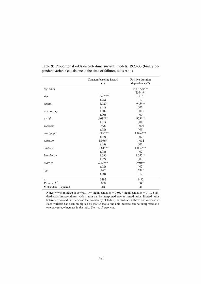
Table 9: Proportional odds discrete-time survival models, 1923-33 (binary de-pendent variable equals one at the time of failure), odds ratios

Constant baseline hazard(1)

Positive durationdependence (2)

log(time) 2477.729***(2374.94)

size 1.640*** .916(.26) (.17)

capital 1.020 .945***(.01) (.02)

reserve dep 1.002 1.001(.00) (.00)

gvtbds .961*** .953***(.01) (.01)

secloans .998 1.009(.02) (.01)

mortgages 1.088*** 1.084***(.02) (.02)

other re 1.076* 1.054(.05) (.07)

othloans 1.064*** 1.064***(.02) (.02)

bankhouse 1.036 1.055**(.02) (.03)

rearngs .942*** .950**(.02) (.02)

age .692 .638*(.00) (.17)

n 1492 1492Prob > chi2 .000 .000McFadden R-squared .18 .41

Notes: *** significant at a = 0.01, ** significant at a = 0.05, * significant at a = 0.10. Stan-dard errors in parentheses. Odds ratios can be interpreted here as hazard ratios. Hazard ratiosbetween zero and one decrease the probability of failure; hazard ratios above one increase it.Each variable has been multiplied by 100 so that a one unit increase can be interpreted as aone percentage increase in the ratio. Source: Statements.

42

7.4 Problems with unit banking

In the 1920s all Chicago state banks operated under the unit banking system; they were not allowed

to open branches as Illinois banking law forbade it. Problems linked to unit banking were numerous.

The main reason branch banking is usually thought of as an advantage is that it increases portfolio

diversification. Branch banking can be contrasted to group or chain-banking as branches of the same

bank can pool their assets and liabilities together. When there is a liquidity shortage at one of the banks

in a chain, other member banks cannot simply transfer funds to that bank for help, a problem which does

not even arise in the branch banking system. This may partly explain the collapse of the Bain chain in

June 1931 which triggered the banking crisis at that time (James, 1938, p. 994).

Yet the lack of portfolio diversification was not necessarily directly due to the unit banking system.

Indeed, Rodkey points to the fact that many small bankers prior to the Depression felt a moral duty to

“meet all demands for good local loans” (Rodkey, 1944, p. 4). It also seems that the lack of portfolio

diversification was not the only disadvantage of unit banking. Rodkey blamed this system for fostering

the incompetence of bank managers:

“This system leads naturally to a multiplicity of small banks under local control, ownedlocally, and operated usually by citizens of the home community who may or may not havesome knowledge of the fundamental principles of sound banking” (Rodkey, 1935, p. 147).

Thus, by triggering the establishment of many small banks, unit banking made it easier for inexpe-

rienced bankers to become managers.64 Rodkey also pointed out that little attention was given to the

ability of the borrower to meet his interest payments (ibid., p. 122).

The ease with which almost any kind of manager could open a small community bank and the result-

ing lack of experience of such unit bank managers in Illinois stand out as potentially serious problems

when the Chicago mortgage boom is taken into account.

64Nevertheless, the debate on branch banking has not completely ended. So far, at least four studies have shown that thebranch banking system was detrimental to bank survival during the Depression. While Calomiris & Wheelock (1995) concedethat it has usually been a good thing in U.S. history, they find that such was not the case in the Great Depression. Some ofthe largest branching networks collapsed in the 1930s, which may have been due to a form of moral hazard: branching banksthought they were better protected against local risk, and thus were less careful with their asset management (see also Carlson(2001)). Calomiris & Mason (2003) confirm the negative effect of branch banking, and so does Carlson (2001). On the otherhand, Mitchener (2005) finds a positive effect, while Gambs (1977) finds no effect at all.

43

7.5 Bank size

This appendix deals with the problem of bank size. First of all, it should be noted that bank size is not

necessarily a problem in the sense that it does not necessarily introduce bias in the results. Most of the

time it does not because authors make a point of studying mainly financial ratios. When looking at the

main indicators of bank size (total assets, total capital, and sometimes total deposits), it appears that

larger banks did tend to have a higher survivor rate. However, one of the aims of this paper is precisely

to show that this was certainly not the only reason for their survival (of course, it may be that there is a

correlation between larger bank size and better management practice). Table 10 shows the failure rate

per size group, using the whole population of 193 banks (see notes below Table 2).

Table 10: Relationship between bank size and failure rate, June 1929 -June 1933

Total Capital Number of banks Number of failures Failure rate(%)

Less than $250,000 87 77 89

$250,001 -$375,000

16 14 88

$375,001 -$800,000

45 36 80

More than$800,000

45 33 73

Notes: There are 193 banks in total in this table because they include those that arenot part of any cohort, eg. those that failed between the chosen windows of failure.The actual bank total for June 1929 as the sum of each cohort is 131. Source:Statements.

From this table it appears that there is indeed a relationship between size and failure, although this

relationship is not very strong. True, whether large or small, banks had a high failure rate, always above

70 percent. Nevertheless, it is still noticeable that banks with less than $250,000 in capital had 89 percent

chances of failing, whereas banks whose capital went beyond $800,000 “only” had a failure rate of 73

percent. Looking at total assets for the whole period, the differences are even more striking (see Figure

14).

7.6 Mortgage growth rates

One may wonder how a non-increasing share of real estate to total assets may have substantially weak-

ened banks. First note that the data only start in 1923, which as shown in Section 5 was already some

way into the boom. The real estate boom may also be hidden by the fact that banks grew significantly

44

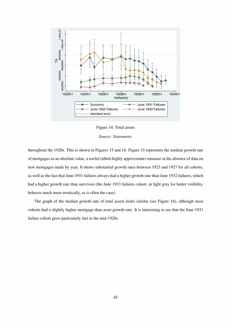
2000

00040

0000

0 6000

00080

0000

0 1.00

e+07

1.20

e+07

TA



Figure 14: Total assets

Source: Statements.

throughout the 1920s. This is shown in Figures 15 and 16. Figure 15 represents the median growth rate

of mortgages as an absolute value, a useful (albeit highly approximate) measure in the absence of data on

new mortgages made by year. It shows substantial growth rates between 1923 and 1927 for all cohorts,

as well as the fact that June 1931 failures always had a higher growth rate than June 1932 failures, which

had a higher growth rate than survivors (the June 1933 failures cohort, in light grey for better visibility,

behaves much more erratically, as is often the case).

The graph of the median growth rate of total assets looks similar (see Figure 16), although most

cohorts had a slightly higher mortgage than asset growth rate. It is interesting to see that the June 1931

failure cohort grew particularly fast in the mid-1920s.

45

−.1

0.1

.2.3


Survivors June 1931 FailuresJune 1932 Failures June 1933 Failures

Figure 15: Median growth rate of mortgages (six months to six months)

Source: Statements.

−.2

−.1

0.1

.2


Survivors June 1931 FailuresJune 1932 Failures June 1933 Failures

Figure 16: Median growth rate of total assets (six months to six months)

Source: Statements.

46

7.7 Survival model for the liability side

Table 11 provides a discrete-time proportional odds model for the liability side of bank balance sheets.

This model was chosen for the same reasons as in Appendix 7.3. The focus is on the years 1929-

1933. As borrowed funds and deposit losses are highly correlated, they were entered separately in the

regression. All items are ratios to total liabilities and equity except for retained earnings to net worth.

Table 11: Discrete-time proportional odds estimation, 1929-33 (bi-nary dependent variable equals one at the time of failure), oddsratios

(1) (2)

Capital 1.008 .982(.01) (.01)

Retained earnings .939*** .941***(.02) (.02)

Borrowed funds 1.043***(.01)

Total deposits .972***(.01)

n 885 885Prob > chi2 .000 .000Likelihood -284.22 -287.12

Notes: *** significant at a = 0.01, ** significant at a = 0.05, * significant ata = 0.10. Standard errors in parentheses. Odds ratios can be interpreted hereas hazard ratios. Hazard ratios between zero and one decrease the probabilityof failure; hazard ratios above one increase it. Each variable has been multi-plied by 100 so that a one unit increase can be interpreted as a one percentageincrease in the ratio.Source: Statements.

47

WHAT CAUSED CHICAGO BANK FAILURES IN THE GREAT DEPRESSION ... 22 (Postel-Vinay, April 20… ·...

Documents

Transcript of WHAT CAUSED CHICAGO BANK FAILURES IN THE GREAT DEPRESSION ... 22 (Postel-Vinay, April 20… ·...