Western Washington Hydrology Model · PDF fileWESTERN WASHINGTON HYDROLOGY MODEL Prepared by...

Western WashingtonHydrology Model

User’s Manual

June 2001Publication Number 01-10-040

To download the Western Washington Hydrology Modeland the electronic version of this User’s Manual,

please visit our website at:

http://www.ecy.wa.gov/programs/wq/links/stormwater.html

If you have questions about the WWHM, please contact:

Foroozan Labib, Environmental EngineerDepartment of EcologyWater Quality Program

(360) [email protected]

The Department of Ecology is an equal opportunity agency and does not discriminate on thebasis of race, creed, color, disability, age, religion, national origin, sex, marital status, disabledveteran's status, Vietnam Era veteran's status, or sexual orientation.

If you have special accommodation needs or require this document in an alternative format,please call Donna Lynch at (360) 407-7529. The TDD number is (306) 407-6006. Email can besent to [email protected]

WESTERN WASHINGTONHYDROLOGY MODEL

Prepared by

AQUA TERRA ConsultantsIn Association with

Otak, Inc.

User’s Manual

W E S T E R N WA S H I N G T O N H Y D R O LO G Y M O D E L Table of Contents

Introduction ................................................................................................. 1

Step 1 ........................................................................................................... 3

Step 2 .........................................................................................................10

Step 3 .........................................................................................................17

Step 4 .........................................................................................................18

Step 5 .........................................................................................................19

Step 6 .........................................................................................................21

Step 7 .........................................................................................................22

Step 8 .........................................................................................................25

Report .........................................................................................................26

Analysis .......................................................................................................31

Graphing Capability ....................................................................................34

W E S T E R N WA S H I N G T O N H Y D R O LO G Y M O D E L Introduction

Page 1

Purpose Size storm water control facilities that mitigate the effects of increased runoff (peak

discharge, duration, and volume) from a proposed development on a stream using

a computer model that represents the following:• a uniform method for western Washington

• a more accurate method than single event design storms

• an easy–to–use software package

The computer program is based on:

• continuous simulation hydrology (HSPF)

• actual recorded precipitation• measured pan evaporation

• historic vegetation

• regional HSPF parameters

Parameter values can be modified for local conditions.

• Windows 9x/ME/2000 with 50 MB uncompressed hard drive space• Internet access (only required for downloading program, not required for

executing WWHM)

• Pentium 2 or faster processor (desirable)

• Color monitor (desirable)

• Site location or street address

• Aerial distribution of existing site soil by category (outwash, till, wetland)• Aerial distribution of proposed development (residences, streets/sidewalks,

landscaped areas) in relation to the soil categories

• At least a first approximation for stormwater control facility (stage (ft), storage

(ac-ft), discharge (cfs))

• Assemble site characteristics

Download the program. The program is available at ftp://www.ecy.wa.gov/ftp

anon/wq/. The user needs to download the following files: setup.exe,ehm.cab, setup.lst, infoandassumptions.doc, and “name of the county”co.exe

(name of the county in which the project is located, i.e., kingco.exe)

• After download is completed, user needs to run setup.exe file. This will create

c:\program files\ehm folder. Now the user can access and run the model from

c:\program files\ehm folder by double clicking on the ehm.exe file. However,the user must load the map file for the county of the project by double

clicking on the county’s name and unzipping the map information for that

county. This county’s map files have to be in c:\program\wwhm\map\directory.

• Step through each of the screens• Review performance of stormwater control facility

• If facility meets requirements, stop; otherwise:

• adjust stage–storage–discharge relationship of facility

• review performance of facility

ComputerRequirements

Before Startingthe Program

Procedure

W E S T E R N WA S H I N G T O N H Y D R O LO G Y M O D E L Introduction

Page 2

• WWHM is available through the Washington Department of Ecology

controlled web site

• The program is downloaded to the user’s personal computer and isautomatically executed

• WWHM comes with default values for most input parameters

• Tool bars are available for saving or reloading project data, editing default

parameter values, and finding help concerning the program• The following pages illustrate the steps required to run the WWHM, as they

would appear on screen (except for this User’s Manual’s explanatory graphics)

Step 1

Page 3

W E S T E R N WA S H I N G T O N H Y D R O LO G Y M O D E L

A To use Zoom to Rectangle, left click and draw a rectangle in the maparea to view a specific location in the map.

B Move Center.

C The Zoom Out button allows the user to view a larger area at asmaller scale.

D The Zoom In button allows the user to view a smaller area at a largerscale.

E The Reset button allows the user to view the full map after any zoomoperations.

F The user can right-click on a street and it will be identified in theseboxes. (The crosshairs must be exactly on the street line.)

G Drag the Flag over the map and drop in desired location. It allows theuser to select a particular project site within the map.

GETTING STARTED

THE BUTTONS

A Pull down menu

B Buttons

C Map Area

D Forward/Back Navigation buttons

B

C

A

D

D

A D FECB G

Step 1

Page 4


PULL DOWN MENU

Load Project Will automatically take you to the directoryc:\program files\wwhm\.

Save Project As Any new project should be saved the first time using thiscommand.

Note: Projects may not work if saved in network folders on other computers.

File Name The program will not work if the project name includes any nonalphanumeric characters. It will accept spaces in between alphanumericcharacters, but not anything else.

Export Timeseries Will export time series files to a specified filename under asubdirectory. This option will be available only after completing runoff andflood frequency analysis. See page 23 for further information.

Location Editor This option will be available once the project site is selectedin the county selected by dragging and dropping the flag. See next page forlocation editor screen.

Change Criteria When this option is chosen, you get the following dialog box:

File

Tools

Using these three dialog boxes, any range of flow can be selected for flowduration analysis.

Allowable post developed flow discharge durationPredeveloped flow discharge duration X 100=

Step 1

Page 5


Location Editor

HSPF parameters for each PERLND type which describe various hyrologicfactors that influence runoff. See next page for further discussion.

Previous land categories represented by PERLNDs in WWHM.See next page for further discussion.

User can edit these values if better representative values are known.

Update Updates the table if values are edited.

Done Will take user to previous screen.

Reset to defaults This will automatically set the values to default.

Done Once the four values are set, this will update the values.

Step 1

Page 6


PERLND AND IMPLND PARAMETER VALUES.

PERLNDParameters

In WWHM (and HSPF), pervious land categories are represented by PERLNDs;

impervious land categories (EIA) by IMPLNDs. An example of a PERLND isa till soil covered with forest vegetation. This PERLND has a unique set of

HSPF parameter values. For each PERLND there are 16 parameters that

describe various hydrologic factors that influence runoff. These range from

interception storage to infiltration to active groundwater evapotranspiration.Only four parameters are required to represent IMPLND.

The PERLND and IMPLND parameter values to be used in the WWHM are

listed below. These values are based on regional parameter values developed bythe U.S. Geological Survey for watersheds in western Washington (Dinicola,

1990) plus additional HSPF modeling work conducted by AQUA TERRA

Consultants.

TF TP TL OF OP OL SF SP SL

Name

LZSN 4.5 4.5 4.5 5.0 5.0 5.0 4.0 4.0 4.0

INFILT 0.08 0.06 0.03 2.0 1.6 0.80 2.0 1.8 1.0

LSUR 400 400 400 400 400 400 100 100 100

SLSUR 0.10 0.10 0.10 0.10 0.10 0.10 0.001 0.001 0.001

KVARY 0.5 0.5 0.5 0.3 0.3 0.3 0.5 0.5 0.5

AGWRC 0.996 0.996 0.996 0.996 0.996 0.996 0.996 0.996 0.996

INFEXP 2.0 2.0 2.0 2.0 2.0 2.0 10.0 10.0 10.0

INFILD 2.0 2.0 2.0 2.0 2.0 2.0 2.0 2.0 2.0

BASETP 0.0 0.0 0.0 0.0 0.0 0.0 0.0 0.0 0.0

AGWETP 0.0 0.0 0.0 0.0 0.0 0.0 0.7 0.7 0.7

CEPSC 0.20 0.15 0.10 0.20 0.15 0.10 0.18 0.15 0.10

UZSN 0.5 0.4 0.25 0.5 0.5 0.5 3.0 3.0 3.0

NSUR 0.35 0.30 0.25 0.35 0.30 0.25 0.50 0.50 0.50

INTFW 6.0 6.0 6.0 0.0 0.0 0.0 1.0 1.0 1.0

IRC 0.5 0.5 0.5 0.7 0.7 0.7 0.7 0.7 0.7

LZETP 0.7 0.4 0.25 0.7 0.4 0.25 0.8 0.8 0.8

PERLND types:

TF = Till ForestTP = Till PastureTL = Till LawnOF = Outwash ForestOP = Outwash Pasture

OL = Outwash LawnSF = Saturated ForestSP = Saturated PastureSL = Saturated Lawn

Step 1

Page 7


IMPLNDParameters

PERLND parameters:

LZSN = lower zone storage nominal (inches)INFILT = infiltration capacity (inches/hour)LSUR = length of surface overland flow plane (feet)SLSUR = slope of surface overland flow plane (feet/feet)KVARY = groundwater exponent variable (inch-1)AGWRC = active groundwater recession constant (day-1)INFEXP = infiltration exponentINFILD = ratio of maximum to mean infiltrationBASETP = base flow evapotranspiration (fraction)AGWETP = active groundwater evapotranspiration (fraction)CEPSC = interception storage (inches)UZSN = upper zone storage nominal (inches)NSUR = roughness of surface overland flow plane (Manning’s n)INTFW = interflow indexIRC = interflow recession constant (day-1)LZETP = lower zone evapotranspiration (fraction)

A more complete description of these PERLND parameters is found in the

HSPF User Manual (Bicknell et al, 1997).

PERLND parameter values for other additional soil/vegetation categories will

be investigated and added to the EHM, as appropriate.

IMPLND parameters:

LSUR = length of surface overland flow plane (feet)SLSUR = slope of surface overland flow plane (feet/feet)NSUR = roughness of surface overland flow plane (Manning’s n)RETSC = retention storage (inches)

EIA

Name

LSUR 100

SLSUR 0.01

NSUR 0.10

RETSC 0.10

Step 1

Page 8


A more complete description of these IMPLND parameters is found in the

HSPF User Manual (Bicknell et al, 1997).

The PERLND and IMPLND parameter values will be transparent to the

general user. The advanced user will have the ability to change the value of a

particular parameter for that specific site. However, such changes will berecorded in the WWHM output.

Surface runoff and interflow will be computed based on the PERLND andIMPLND parameter values. Groundwater flow will not be computed, as it is

assumed that there is no groundwater flow from small catchments that reach the

surface to become runoff. This is consistent with King County procedures (King

County, 1998).

Step 1

Page 9


Help

Step 2

Page 10


Enter projectinformation inthese fields.

After entering project information, the user has to select Standard Residentialor Non–Standard Commercial for developed conditions before entering anyother values. The user has the option to choose one or the other, but notboth. If there are both types of development available, the user has to analyzeseparately. See page 15 for further detail on development land use data.

STANDARD RESIDENTIAL OPTION

Enter Predeveloped Acres appropriately.

Choose Vegatation type appropriately. Since pasturecreates less runoff, if pasture is chosen, the user willget the following message (see page 14 for furtherdetail on vegetation data):

Step 2

Page 11


User has the option to choose one or anycombination of basins. See page 17 for furtherinformation.

Information in this dialog boxrepresents developed conditions. Seepage 15 for further information onstandard residential.

Lot Acres Enter lot acres appropriately

Note: Total acreage of A/B soils enteredunder predeveloped acres should matchthe acreage of A/B soils entered under

developed conditions, and the total acreage of C soils entered underpredeveloped acres should match the acreage of C soils entered underdeveloped conditions; i.e., standard residential or non-standard/commercial,whichever the type of development. Otherwise, user will get a warningmessage:

Streets/Sidewalks Input impervious area streets and sidewalks within thepublic row which used to be A/B soils or C soils.

Number of Lots Enter total number of lots in the standard residential area.

Pavement Credit and Roof Runoff Credits Select these options if applicable.To select, click on the buttons to make them green and then enter percentages.See page 16 for further information.

Enter an Estimated Pond Area. This area isconsidered part of the post-developed area andis modeled impervious in the “developed without

facility” scenario. It is replaced by the pond in the “developed with facility”scenario.

Note: Pond area must be reentered if the user switches from standard to non-standard or vice-versa.

Step 2

Page 12


NON–STANDARD COMMERCIAL OPTION

To select the Non–Standard Commercial option,click on the button to make it green.

User has the option to choose one or anycombination of Basins. For each of the options

selected, user has to enter the predeveloped and developed data. See page 17for further information.

Enter values appropriately. See page 17for further information. Total Type A/B

soils and Type C acreage should match under predeveloped and post-developed conditions.

The only runoff credit availabe in non–standard/commercial is Porous Pavement. Click there if

applicable. To select this option, make the button is green. See page 16 forfurther information.

Step 2

Page 13


As with soil type, vegetation types greatly influence the rate and timing of the

transformation of rainfall to runoff. Vegetation intercepts precipitation,

increases its ability to percolate through the soil, and evaporates and transpires

large volumes of water that would otherwise become runoff.

The WWHM will represent the vegetation of western Washington with three

predominant vegetation categories: forest, pasture, and lawn (also known as grass).

Forest vegetation is represented by the typical second growth Douglas fir found in

the Puget Sound lowlands. Forest has a large interception storage capacity. This

means that a large amount of precipitation is caught in the forest canopybefore reaching the ground and becoming available for runoff. Precipitation

intercepted in this way is later evaporated back into the atmosphere. Forest

also has the ability to transpire moisture from the soil via its root system. This

leaves less water available for runoff.

Pasture vegetation is typically found in rural areas where the forest has been

cleared and replaced with shrub or grass lots. Some pasture areas may be used

to graze livestock. The interception storage and soil evapotranspiration capacitiesof pasture are less than forest. Soils may have also been compressed by mechanized

equipment during clearing activities. Livestock can also compact soil. Pasture areas

typically produce more runoff (particularly surface runoff and interflow) than

forest areas.

Lawn vegetation is representative of the suburban vegetation found in typical

residential developments. Soils have been compacted by earth movingequipment, often with a layer of top soil removed. Sod and ornamental bushes

replace native vegetation. The interception storage and evapotranspiration of

lawn vegetation is less than pasture. More runoff results.

Predevelopment land conditions are assumed to be forest, although the user

has the option of specifying pasture if there is documented evidence that

pasture vegetation was native to the predevelopment site (if this option is used,

pasture predevelopment vegetation will be recorded in the WWHM output).

Forest vegetation is represented by specific HSPF parameter values that represent

the forest hydrologic characteristics. As described above, the existing regionalHSPF parameter values for forest are based on undisturbed second-growth

Douglas fir forest found today in western Washington lowland watersheds.

Postd-evelopment vegetation will reflect the new vegetation planned for the site.

The user has the choice of forest, pasture, and landscaped vegetation. Forest

and pasture are only appropriate for post-development vegetation in parcels

separate from standard residential or non-standard residential/commercial. The

pervious land portion of the standard residential and non-standard residential/commercial is assumed to be covered with lawn vegetation, as described above.

VEGETATION DATA

Step 2

Page 14


Development land use data are used to represent the type of development

planned for the site and are used to determine the appropriate size of therequired stormwater mitigation facility.

For the purposes of the WWHM in western Washington, developed land isdivided into two major categories:

1. standard residential, and

2. non-standard residential/commercial.

Standard residential development makes specific assumptions about the

amount of impervious area per lot and its division between driveways and

rooftops. Streets and sidewalk areas are input separately. Ecology has selected

a standard impervious area of 4,200 square feet per residential lot, with 1,000square feet of that as driveway, walkway, and patio area, and the remainder as

rooftop area.

Impervious, as the name implies, allows no infiltration of water into the

pervious soil. All runoff is surface runoff. Impervious land typically consists

of paved roads, sidewalks, driveways, and parking lots. Roofs are also

hopefully impervious.

For the purposes of hydrologic modeling, only effective impervious area is

categorized as impervious. Effective impervious area (EIA) is the area wherethere is no opportunity for surface runoff from an impervious site to infiltrate

into the soil before it reaches a conveyance system (pipe, ditch, stream, etc.).

An example of an EIA is a shopping center parking lot where the water runs

off the pavement and directly into a catch basin where it then flows into a pipe

and eventually to a stream. In contrast, some homes with impervious roofs collectthe roof runoff into roof gutters and send the water down downspouts. When

the water reaches the base of the downspout it can be directed either into a pipe

or dumped on a splash block. Roof water dumped on a splash block then has the

opportunity to spread out into the yard and soak into the soil. Such roofs are notconsidered to be effective impervious area. For hydrologic modeling purposes,

runoff credits are given to developments that contain houses that have roof runoff

systems that disperse roof runoff and allow it to drain into the soil. A runoff

credit is given by assuming in the modeling that the roof area behaves

hydrologically as lawn rather than EIA.

The non-effective impervious area uses the adjacent or underlying soil and

vegetation properties. Vegetation often varies by the type of land use. Standardresidential and non-standard residential/commercial are both assumed to have

lawn as their typical pervious area vegetation.

The assumption is made in the WWHM that the EIA equals the TIA (total

impervious area). This is consistent with King County’s determination of EIA

DEVELOPMENT LAND USE DATA

StandardResidential

Step 2

Page 15


acres for new developments. Where appropriate, the TIA can be reduced through

the use of runoff credits (more on that below).

For standard residential developments the user will input the TIA in the public

right-of-way (streets and sidewalks). In addition, the user will input the

number of residential lots and the number of acres associated directly withthese residential lots (public right-of-way acreages and non-residential lot

acreages excluded). The number of residential lots and the associated number

of acres will be used to compute the average number of residential lots per

acre. This number will be used to compute the average amount of imperviousarea per residential lot. This value together with the number of residential lots

and the public right-of-way TIA will be used by the model to calculate the

total TIA for the proposed development.

Runoff credits will be given reducing runoff from standard residential lots.

Runoff credits can be obtained using any or all of the three methods described

below:

1. Infiltrate roof runoff2. Disperse roof runoff

3. Use porous pavement for driveway areas

Credit is given for disconnecting the roof runoff from the development’s

stormwater conveyance system and infiltrating on the individual residential

lots. The WWHM assumes that this infiltrated roof runoff does not contribute to

the runoff flowing to the stormwater detention pond site. It disappears from the

system and does not have to be mitigated.

Credit is also given for disconnecting the roof runoff from the development’s

stormwater conveyance system and dispersing it on the surface of individuallots. This runoff is assumed to be the equivalent of runoff from lawn

vegetation.

The third option for runoff credit is the use of porous pavement for private

driveway areas. Specific HSPF parameters for porous pavement have not been

developed for the WWHM. Ecology has made the assumption that porous

pavement runoff is equivalent to the conversion of 147 square feet (4200*0.035)

of impervious area to lawn vegetation. This assumption is used in the WWHMcalculations.

Forest and pasture vegetation areas are only appropriate for separate undevelopedparcels dedicated as open space, wetland buffer, or park within the total area of the

standard residential development.

Pavement orRoof Runoff Credits

Step 2

Page 16


Non-standard residential/commercial development includes residential

developments for which the standard residential development assumptions are

inappropriate, plus commercial, industrial, schools, roads, multi-familyresidential (apartments, condos), and other non-single family residential

developments. For this type of development the user will input the roof area,

landscaped area, street/sidewalk/parking areas, and any appropriate non-developed

forest and pasture areas. Developed runoff will be calculated based on thesecategories and their areas. The only explicit runoff credit available to the user is

porous pavement for streets, sidewalks, and parking lots. It is specified as a percent

of the total street/sidewalk/parking impervious area. The user can also implicitly

obtain other runoff credits by decreasing roof area and street/sidewalk/parking

areas. This will decrease surface runoff.

Forest and pasture vegetation areas are only appropriate for separate

undeveloped parcels dedicated as open space, wetland buffer, or park withinthe total area of the development.

The WWHM allows the flexibility of routing a portion of the development areaaround a stormwater detention facility and/or having offsite inflow enter the

development area. Three options are available to the user:

1. Design Basin: usual development situation with no offsite inflow and no

flow bypass.2. Bypass: a portion of the development does not drain to a stormwater

detention facility.

3. Offsite Inflow: an upslope area outside the development drains to the

stormwater detention facility in the development.

For each of these options the user inputs the number of acres in the different

categories for the predevelopment and post-development land use. When Offsite

Inflow option is chosen, the user will enter the areas under developed conditionsonly since this offsite area is out of the development. See next page. For each type

of basin being selected, user has to choose Standard Residential or Non–Standard

Commercial before entering any values in the developed areas. The WWHM

computes the runoff from each separately and adds them together, as appropriate,

to check to see if the stormwater standards have been satisfied.

With all of the above information provided by the user, the WWHM computes

the corresponding number of acres of pervious and impervious land and assignsthese acres to specific PERLNDs and IMPLNDs (HSPF-speak for pervious land

categories and impervious land categories) for use by the model in computing

post-development runoff.

Non–StandardResidential/Commercial

Basins

Step 2 and Step 3

Page 17


OFFSITE INFLOW SELECTED

• Entering predeveloped areas will not be an option when Offsite Inflow ischosen.

• User enters the areas values under the Developed Conditions only.

When the Next button is pressed after entering all thevalues, click Yes to Compute Runoff.

Program now computes runoff for predeveloped and developed conditions.Once this dialog box disappears, click on Next to go to the next step.

Step 4

Page 18


PERFORMING ANALYSIS

Perform Click here to compute Flood Frequency and Flood Duration values.When this option is chosen, user will see three graphs progressing in the boxnext to it.

Black Flood frequency values for predeveloped conditions.

Red Flood duration values for predeveloped.

Blue Flood frequency values for post- development without facility.

Flood frequency is computed using USGS standard Log-Pearson Type IIIprocedures rather than assuming a preselected year for a specified floodevent. The flood frequency computations include a regional skew coefficient.The regional skew coefficient is not input by the user, but is determined fromPlate I of Bulletin 17B (the USGS refers to the regional skew coefficient as the“generalized skew coefficient”) for Western Washington. Plate I shows thecoefficient is 0.0 for areas east of the Olympic Mountains and 0.2 for areaswest. These values have been included in the dataset.

Once Flood Frequency and Flood Duration analyses are done, correspondingvalues show up. Note: After this step, if user edits any values in LocationEditor (see page 6), user must compute runoff again by clicking Previousbutton. The program will not update the analysis by itself.

Next Click to go to the next step.

Step 5

Page 19


Infiltration If the facility has infiltration capacity, choose this option byclicking and making the button green. If not, click on Add Table From File.Enter Facility Name and Type of Facility. (The file can be a *.csv, tab delimited,or a text file with the numbers separated by spaces.)

Note: When manually entering numbers in this table, decimal numbers lessthan one must be preceded by a zero.

INFILTRATION OPTION

Screen with Infiltration option chosen.

Step 5

Page 20


Enter Facility Name and Type of Facility information.

Add Table From File File should be a CSV (Comma delimited)(*.csv) one. Thefile should have five columns if Infiltration option is chosen, otherwise itshould have four columns.

User should note the following:• When importing or entering values, values should be consistent with the

units in the heading.• The first row of values must be zero.• Stage must increase from one row to the next.• Storage should increase from one row to the next.• Maximum number of total values is 500 (5 x 100 if infiltration option is

chosen) or 400 (4 x 100 if infiltration option is not chosen).• Maximum number of rows is 99.

Next Once finished entering all the values, click here to go to the next step.

Click Yes to compute analysis with pond.

Step 6

Page 21


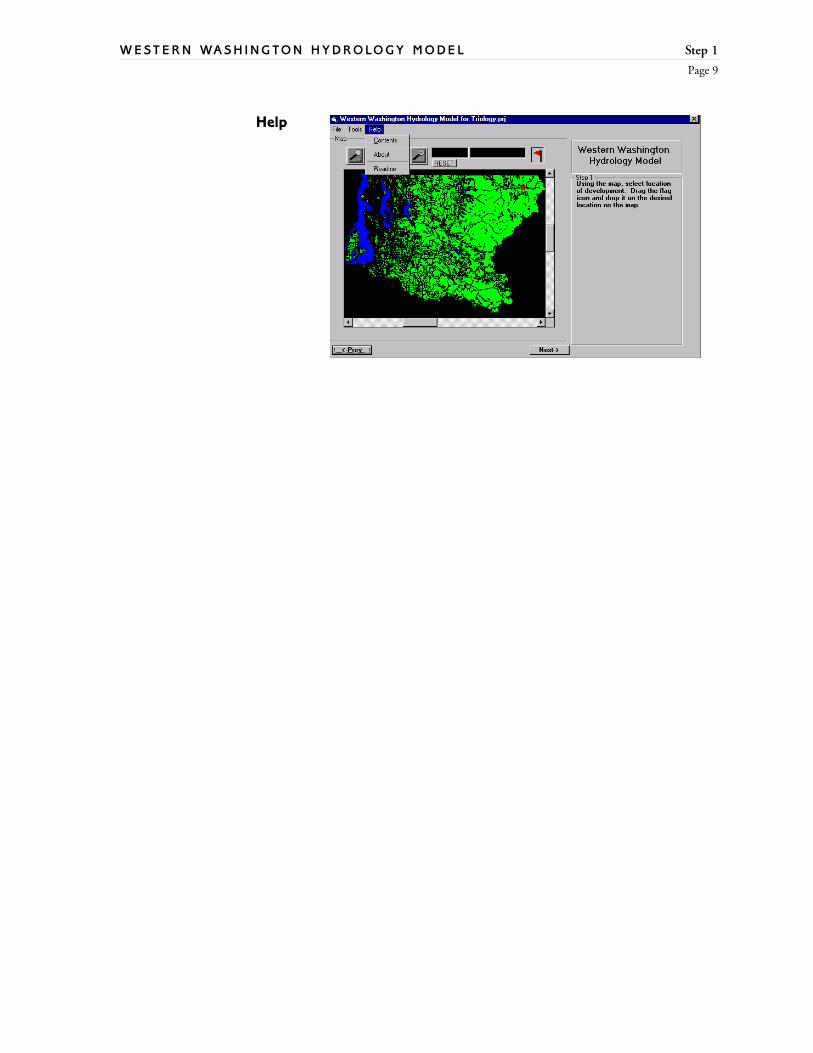
COMPUTING RUNOFF

The program now computes runoff for developed conditions with facility.Once completed, click on Next to go to Step 7.

Step 7

Page 22


Perform Click to see computer peaks with detention facility:

Once the Flood Frequency Analysis is done for Predevelopment, Post-development and Post-development with Detention Facility, user can ExportTimeseries to a specified location:

Time Series User has to choose one at a time. Follow through next threescreen shots.

Browse Click here to give a file name. The program will take the userautomatically to c:\program files\wwhm\data directory. See next screen.

Step 7

Page 23


File Name Enter file name.

Save as type Data is exported to a sequential file for use with HSPF.

Save Click Save when done.

To actually generate the file in the format selected and to save, user must clickhere. See next screen.

Program is generating and saving.

Perform Statistical Analysis Click here to perform Statistical Analysis in Step7 (page 23). See next screen. Anytime if the user edits values under changecriteria (see page 5), the user has to perform statistical analysis again bypressing this button in Step 7 (see page 23). The program will not update theresults automatically.

Step 7

Page 24


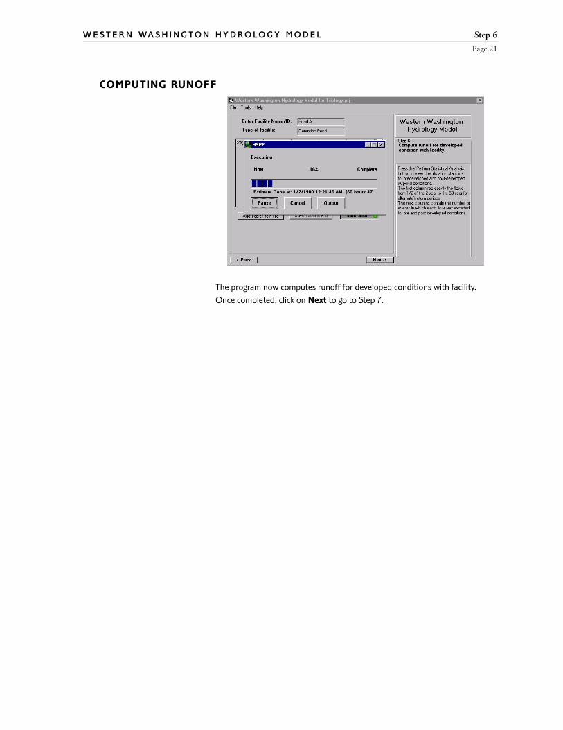
The program rates the detention facility as Pass if none of the values in Column5 fail and if no more than 50% of the values in column 4 exceed 100%. Seenext screen.

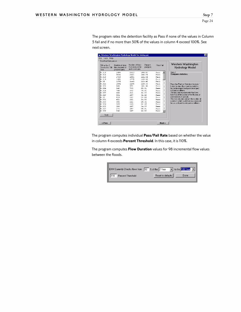
The program computes individual Pass/Fail Rate based on whether the valuein column 4 exceeds Percent Threshold. In this case, it is 110%.

The program computes Flow Duration values for 98 incremental flow valuesbetween the floods.

Step 8

Page 25


The program rated the facility Pass or Fail.

User must save project before clicking on Generate Report.

See next screen.

After highlighting the report, user can click on Copy to copy text to a differentprogram and save file there. See following pages for report.

Click on Print to print the file.

Report

Page 26


REPORT Project File: triology.prjTriology8th Street EastRedmond

Predeveloped Land Use (acres)Basin Outwash Till Saturated/WetlandDesign Basin 1 .5 0

DEVELOPED LAND USETYPE: Residential (acres)BASIN LAND USE OUTWASH TILLDesign Basin Lot Acres .5 .25Design Basin Streets/Sidewalks .5 .25Number of Lots 20

RETURN PERIOD VALUES FOR PREDEVELOPED CONDITIONS (CFS)

YEAR: 2 5 10 25 50 100CFS : 0.03 0.06 0.07 0.1 0.12 0.15

RETURN PERIOD VALUES FOR DEVELOPED CONDITIONS W/ NODETENTION FACILITY(CFS)

YEAR: 2 5 10 25 50 100CFS : 0.99 1.21 1.37 1.57 1.73 1.89

RETURN PERIOD VALUES FOR POST-DEVELOPED CONDITIONS W/POND(CFS)

YEAR: 2 5 10 25 50 100CFS : 0.01 0.03 0.07 0.18 0.36 0.7

DETENTION FACILITY INFORMATION:

NAME OF FACILITY: Pond ATYPE OF FACILITY: Detention Pond

Depth Area Volume Outflow1(ft) (acres) (acre-ft) (cfs)0.00 0.4477 0.0000 0.0000 0.00000.13 0.4530 0.0585 0.0000 0.02280.26 0.4583 0.1177 0.0000 0.02310.39 0.4636 0.1775 0.0000 0.02340.52 0.4690 0.2380 0.0000 0.02360.65 0.4745 0.2992 0.0000 0.02390.78 0.4799 0.3610 0.0000 0.02420.91 0.4854 0.4235 0.0000 0.02451.04 0.4909 0.4867 0.0000 0.02471.17 0.4964 0.5506 0.0000 0.02501.30 0.5020 0.6152 0.0000 0.02531.43 0.5076 0.6804 0.0000 0.02561.56 0.5132 0.7463 0.0011 0.02591.69 0.5189 0.8129 0.0019 0.02621.82 0.5245 0.8803 0.0025 0.02641.95 0.5302 0.9483 0.0029 0.02672.08 0.5360 1.0170 0.0033 0.02702.21 0.5418 1.0865 0.0037 0.02732.34 0.5476 1.1566 0.0040 0.0276

Report

Page 27


2.47 0.5534 1.2275 0.0043 0.02792.60 0.5592 1.2991 0.0046 0.02822.73 0.5651 1.3714 0.0048 0.02852.86 0.5711 1.4445 0.0051 0.02882.99 0.5770 1.5183 0.0053 0.02913.12 0.5830 1.5928 0.0055 0.02943.25 0.5890 1.6680 0.0057 0.02973.38 0.5950 1.7440 0.0060 0.03003.51 0.6011 1.8208 0.0062 0.03033.64 0.6072 1.8983 0.0064 0.03063.77 0.6133 1.9765 0.0065 0.03093.90 0.6195 2.0555 0.0067 0.03124.03 0.6256 2.1353 0.0081 0.03154.16 0.6319 2.2158 0.0098 0.03194.29 0.6381 2.2971 0.0109 0.03224.42 0.6444 2.3792 0.0118 0.03254.55 0.6507 2.4620 0.0126 0.03284.68 0.6570 2.5456 0.0133 0.03314.81 0.6634 2.6300 0.0140 0.03344.94 0.6697 2.7152 0.0146 0.03385.07 0.6762 2.8012 0.0178 0.03415.20 0.6826 2.8880 0.0202 0.03445.33 0.6891 2.9756 0.0219 0.03475.46 0.6956 3.0639 0.0235 0.03515.59 0.7021 3.1531 0.0248 0.03545.72 0.7087 3.2431 0.0261 0.03575.85 0.7153 3.3339 0.6432 0.03615.98 0.7219 3.4255 2.1769 0.03646.11 0.7286 3.5179 4.2367 0.03676.24 0.7353 3.6112 6.7114 0.03716.37 0.7420 3.7053 9.5404 0.03746.50 0.7487 3.8002 12.6837 0.03776.63 0.7555 3.8959 16.1127 0.03816.76 0.7623 3.9925 19.8051 0.03846.89 0.7691 4.0899 23.7434 0.03887.02 0.7760 4.1882 27.9131 0.03917.15 0.7829 4.2873 32.3020 0.03957.28 0.7898 4.3872 36.8997 0.03987.41 0.7967 4.4881 41.6970 0.04027.54 0.8037 4.5897 46.6860 0.04057.67 0.8107 4.6923 51.8596 0.04097.80 0.8178 4.7957 57.2114 0.04127.93 0.8248 4.9000 62.7356 0.04168.06 0.8319 5.0051 68.4271 0.04198.19 0.8390 5.1111 74.2811 0.04238.32 0.8462 5.2180 80.2931 0.04278.45 0.8534 5.3258 86.4591 0.04308.58 0.8606 5.4345 92.7754 0.04348.71 0.8678 5.5441 99.2384 0.04388.84 0.8751 5.6545 105.8450 0.04418.97 0.8824 5.7659 112.5920 0.04459.10 0.8897 5.8782 119.4766 0.04499.23 0.8971 5.9913 126.4960 0.04529.36 0.9045 6.1054 133.6479 0.04569.49 0.9119 6.2204 140.9297 0.04609.62 0.9194 6.3363 148.3391 0.04649.75 0.9268 6.4532 155.8740 0.04679.88 0.9344 6.5709 163.5324 0.047110.01 0.9419 6.6896 171.3123 0.047510.14 0.9495 6.8092 179.2118 0.0479

Report

Page 28


10.27 0.9571 6.9298 187.2291 0.048310.40 0.9647 7.0513 195.3625 0.048610.53 0.9723 7.1737 203.6104 0.049010.66 0.9800 7.2971 211.9713 0.049410.79 0.9877 7.4214 220.4435 0.049810.92 0.9955 7.5467 229.0258 0.050211.05 1.0033 7.6729 237.7166 0.050611.18 1.0111 7.8001 246.5146 0.051011.31 1.0189 7.9283 255.4186 0.051411.44 1.0267 8.0574 264.4273 0.051811.57 1.0346 8.1875 273.5395 0.052211.70 1.0426 8.3186 282.7541 0.052611.83 1.0505 8.4506 292.0698 0.053011.96 1.0585 8.5837 301.4857 0.053412.09 1.0665 8.7177 311.0006 0.053812.22 1.0745 8.8527 320.6136 0.054212.35 1.0826 8.9887 330.3237 0.054612.48 1.0907 9.1257 340.1298 0.055012.61 1.0988 9.2637 350.0311 0.055412.74 1.1070 9.4027 360.0267 0.0558

STATISTICAL ANALYSIS FOR PREDEVELOPEDAND DEVELOPED WITH FACILITY

Analysis from 50% of the 2 Year to the 100 Year.

Flows |# of times |# of times |% developed |Pass/Fail|flow exceeds |flow exceeds |compared to ||predeveloped |developed |predeveloped |

(CFS) | | | |

.02 2405. 2420. 100.62 Pass

.02 2034. 2161. 106.24 Pass

.02 1725. 1981. 114.84 Fail

.02 1481. 1775. 119.85 Fail

.02 1276. 1448. 113.48 Fail

.02 1084. 1196. 110.33 Fail

.02 958. 972. 101.46 Pass

.02 846. 753. 89.01 Pass

.03 748. 552. 73.8 Pass

.03 666. 341. 51.2 Pass

.03 594. 187. 31.48 Pass

.03 519. 112. 21.58 Pass

.03 452. 111. 24.56 Pass

.03 392. 111. 28.32 Pass

.03 339. 110. 32.45 Pass

.04 306. 107. 34.97 Pass

.04 275. 107. 38.91 Pass

.04 246. 107. 43.5 Pass

.04 226. 106. 46.9 Pass

.04 199. 106. 53.27 Pass

.04 178. 106. 59.55 Pass

.04 162. 106. 65.43 Pass

.05 137. 106. 77.37 Pass

.05 123. 104. 84.55 Pass

.05 111. 104. 93.69 Pass

.05 98. 103. 105.1 Pass

.05 88. 101. 114.77 Fail

Report

Page 29


.05 78. 101. 129.49 Fail

.05 73. 100. 136.99 Fail

.05 62. 100. 161.29 Fail

.06 54. 98. 181.48 Fail

.06 52. 97. 186.54 Fail

.06 48. 97. 202.08 Fail

.06 45. 96. 213.33 Fail

.06 43. 96. 223.26 Fail

.06 41. 96. 234.15 Fail

.06 39. 96. 246.15 Fail

.07 34. 96. 282.35 Fail

.07 31. 94. 303.23 Fail

.07 29. 94. 324.14 Fail

.07 27. 94. 348.15 Fail

.07 27. 94. 348.15 Fail

.07 26. 94. 361.54 Fail

.07 23. 94. 408.7 Fail

.07 23. 94. 408.7 Fail

.08 22. 94. 427.27 Fail

.08 22. 94. 427.27 Fail

.08 21. 93. 442.86 Fail

.08 19. 91. 478.95 Fail

.08 17. 91. 535.29 Fail

.08 17. 91. 535.29 Fail

.08 15. 91. 606.67 Fail

.09 15. 91. 606.67 Fail

.09 14. 91. 650. Fail

.09 14. 91. 650. Fail

.09 14. 90. 642.86 Fail

.09 13. 89. 684.62 Fail

.09 12. 89. 741.67 Fail

.09 12. 89. 741.67 Fail

.1 12. 88. 733.33 Fail

.1 11. 87. 790.91 Fail

.1 10. 87. 870. Fail

.1 10. 85. 850. Fail

.1 10. 84. 840. Fail

.1 9. 83. 922.22 Fail

.1 9. 83. 922.22 Fail

.1 9. 83. 922.22 Fail

.11 9. 83. 922.22 Fail

.11 9. 83. 922.22 Fail

.11 9. 83. 922.22 Fail

.11 9. 83. 922.22 Fail

.11 9. 83. 922.22 Fail

.11 9. 83. 922.22 Fail

.11 8. 83. 1037.5 Fail

.12 8. 83. 1037.5 Fail

.12 8. 83. 1037.5 Fail

.12 7. 80. 1142.86 Fail

.12 6. 80. 1333.33 Fail

.12 5. 80. 1600. Fail

.12 5. 80. 1600. Fail

.12 5. 80. 1600. Fail

.12 5. 80. 1600. Fail

.13 5. 80. 1600. Fail

.13 5. 79. 1580. Fail

.13 4. 79. 1975. Fail

.13 4. 79. 1975. Fail

.13 4. 79. 1975. Fail

Report

Page 30


.13 4. 79. 1975. Fail

.13 4. 79. 1975. Fail

.14 4. 79. 1975. Fail

.14 4. 79. 1975. Fail

.14 3. 78. 2600. Fail

.14 3. 78. 2600. Fail

.14 2. 77. 3850. Fail

.14 2. 77. 3850. Fail

.14 1. 75. 7500. Fail

.15 1. 75. 7500. Fail

.15 1. 75. 7500. Fail

.15 1. 75. 7500. Fail

.15 1. 74. 7400. Fail

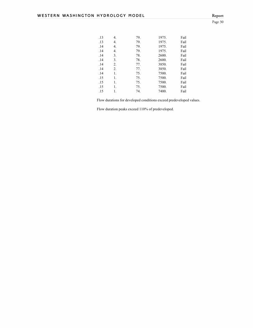
Flow durations for developed conditions exceed predeveloped values.

Flow duration peaks exceed 110% of predeveloped.

Analysis

Page 31


Analyzing WWHMOutput

• In most instances, you will be required to meet a flow duration standard

• Desirable to view output as a graph of discharge versus probability of

exceedence(inverse of return period)

• Analyze curve from bottom to top, and adjust orifices from bottom to top

• Bottom arc corresponds with the discharge from the bottom orifice• reducing the bottom orifice discharge lowers and shortens the

bottom arc

• increasing the bottom orifice raises and lengthens the bottom arc

• Inflection points in the outflow curve occur when additional components(orifices, notches, overflows) become engaged

• lowering the upper orifice moves the breakpoint right on the lower arc

• raising the upper orifice moves the breakpoint left of the lower arc

• Upper arc represents the combined discharge of both orifices. Adjustments

are made to the second orifice as described above for the bottom orifice• Increasing facility volume (via bottom length, width area) moves the entire

curve down and to the left. This is done to control riser overflow conditions.

• Decreasing facility volume (via bottom length, width, area) moves the entire

curve up and to the right. This is done to ensure that the outflow durationcurve extends up to riser overflow.

• The upper tail of the outflow curve will usually not extend all the way to

the riser overflow line. If the riser overflow line does not appear on the

graph, reduce the facility volume until it appears.

Analyzing FlowDuration Curves

Analysis

Page 32


Flow DurationStandard (example)

Observation

1. First arc crosses too high

2. Transition point too far left

3. Second arc too high

4. Second arc stops short of overflow

Refinement

1. Reduce bottom orifice diameter

2. Lower second orifice

3. Reduce second orifice diameter4. Reduce volume of facility if after the above refinements, the second arc still

stops short of the overflow

When required to meet discharge standard, look at the results and adjust

orifice elevation and/or size in a manner similar to that described for the

duration standard output evaluation.

Analysis

Page 33


Peak DischargeStandard (example)

Refinements should be made in small increments. Refine one structure at a time,until you are familiar with the process and the results that you can expect with any

one refinement.

Start adjustments by refining the structure controlling the low flow discharge and

duration. Proceed to the next higher structure after achieving satisfactory results

with the lower structure.

Graphing Capability

Page 34


The following is a description of the WWHM graphing capabilities,

including screenshots.

The flow frequency and duration analysis must be performed in the WWHMbefore the graph will function.

From the Graph Menu, choose from three types of graphs:· Hydrograph· Flow Frequency· Duration Analysis

Hydrograph:

In the Hydrograph Setup, the user must choose which dataset(s) to graph, theinterval and the beginning and end dates to graph.

Also the user must specify whether mean/average or max/peak values areused.

Example If the graph is of monthly values for a number of years, each monthcan be represented by either the maximum flow value for that month or themean/average flow value during that month.

GRAPHING CAPABILITY

Graphing Capability

Page 35


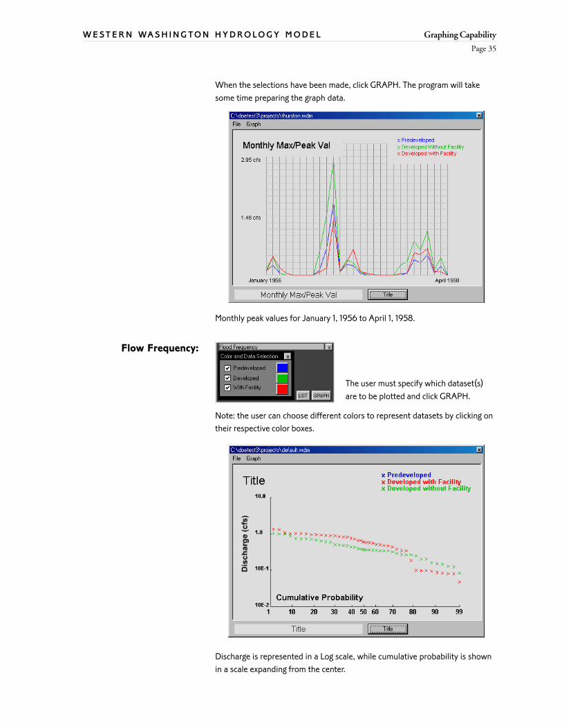
When the selections have been made, click GRAPH. The program will takesome time preparing the graph data.

Flow Frequency:

Monthly peak values for January 1, 1956 to April 1, 1958.

The user must specify which dataset(s)are to be plotted and click GRAPH.

Note: the user can choose different colors to represent datasets by clicking ontheir respective color boxes.

Discharge is represented in a Log scale, while cumulative probability is shownin a scale expanding from the center.

Graphing Capability

Page 36


Duration Analysis The Duration analysis uses datasets for pre developed and developed withfacility only.

Discharge is represented as 1/2 the 2 year return value* to the 50 year return value.*

100 points represent the percentage of flow values that exceed 100 intervalsbetween the 1/2 2 year and 50 year values.

From the File Menu, the user can print the graph or export it to a Bitmap(bmp), Windows Metafile (emf) or a Jpeg (jpg) file.

*These values can be adjusted in the WWHM.

Western Washington Hydrology Model · PDF fileWESTERN WASHINGTON HYDROLOGY MODEL Prepared by...

Documents

Transcript of Western Washington Hydrology Model · PDF fileWESTERN WASHINGTON HYDROLOGY MODEL Prepared by...