LAND AND WATER

Western Port sediment supply, seagrass interactions and remote sensing

Scott N Wilkinson, Janet M Anstee, Klaus D Joehnk, Fazlul Karim, Zygmunt Lorenz, Mark Glover, Rhys Coleman

ii

Citation Wilkinson SN, Anstee JM, Joehnk KD, Karim F, Lorenz Z, Glover M, Coleman R. 2016. Western Port sediment supply, seagrass interactions and remote sensing. Report to Melbourne Water. CSIRO, Australia.

Copyright and disclaimer © 2016 Melbourne Water.

Important disclaimer CSIRO advises that the information contained in this milestone report comprises general statements based on scientific research. The reader is advised and needs to be aware that such information may be incomplete or unable to be used in any specific situation. No reliance or actions must therefore be made on that information without seeking prior expert professional, scientific and technical advice. To the extent permitted by law, CSIRO (including its employees and consultants) excludes all liability to any person for any consequences, including but not limited to all losses, damages, costs, expenses and any other compensation, arising directly or indirectly from using this milestone report (in part or in whole) and any information or material contained in it.

1

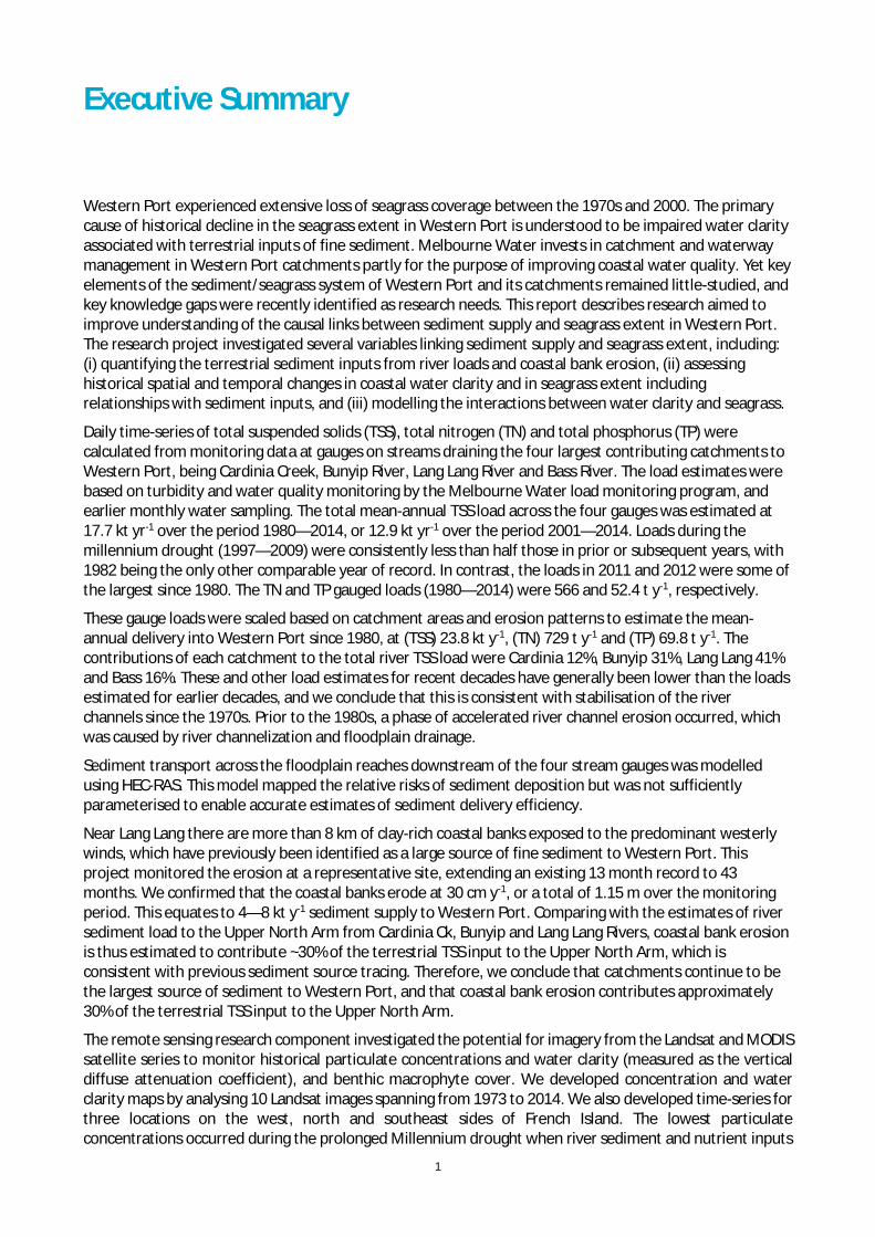
Executive Summary

Western Port experienced extensive loss of seagrass coverage between the 1970s and 2000. The primary cause of historical decline in the seagrass extent in Western Port is understood to be impaired water clarity associated with terrestrial inputs of fine sediment. Melbourne Water invests in catchment and waterway management in Western Port catchments partly for the purpose of improving coastal water quality. Yet key elements of the sediment/seagrass system of Western Port and its catchments remained little-studied, and key knowledge gaps were recently identified as research needs. This report describes research aimed to improve understanding of the causal links between sediment supply and seagrass extent in Western Port. The research project investigated several variables linking sediment supply and seagrass extent, including: (i) quantifying the terrestrial sediment inputs from river loads and coastal bank erosion, (ii) assessing historical spatial and temporal changes in coastal water clarity and in seagrass extent including relationships with sediment inputs, and (iii) modelling the interactions between water clarity and seagrass.

Daily time-series of total suspended solids (TSS), total nitrogen (TN) and total phosphorus (TP) were calculated from monitoring data at gauges on streams draining the four largest contributing catchments to Western Port, being Cardinia Creek, Bunyip River, Lang Lang River and Bass River. The load estimates were based on turbidity and water quality monitoring by the Melbourne Water load monitoring program, and earlier monthly water sampling. The total mean-annual TSS load across the four gauges was estimated at 17.7 kt yr-1 over the period 1980—2014, or 12.9 kt yr-1 over the period 2001—2014. Loads during the millennium drought (1997—2009) were consistently less than half those in prior or subsequent years, with 1982 being the only other comparable year of record. In contrast, the loads in 2011 and 2012 were some of the largest since 1980. The TN and TP gauged loads (1980—2014) were 566 and 52.4 t y-1, respectively.

These gauge loads were scaled based on catchment areas and erosion patterns to estimate the mean-annual delivery into Western Port since 1980, at (TSS) 23.8 kt y-1, (TN) 729 t y-1 and (TP) 69.8 t y-1. The contributions of each catchment to the total river TSS load were Cardinia 12%, Bunyip 31%, Lang Lang 41% and Bass 16%. These and other load estimates for recent decades have generally been lower than the loads estimated for earlier decades, and we conclude that this is consistent with stabilisation of the river channels since the 1970s. Prior to the 1980s, a phase of accelerated river channel erosion occurred, which was caused by river channelization and floodplain drainage.

Sediment transport across the floodplain reaches downstream of the four stream gauges was modelled using HEC-RAS. This model mapped the relative risks of sediment deposition but was not sufficiently parameterised to enable accurate estimates of sediment delivery efficiency.

Near Lang Lang there are more than 8 km of clay-rich coastal banks exposed to the predominant westerly winds, which have previously been identified as a large source of fine sediment to Western Port. This project monitored the erosion at a representative site, extending an existing 13 month record to 43 months. We confirmed that the coastal banks erode at 30 cm y-1, or a total of 1.15 m over the monitoring period. This equates to 4—8 kt y-1 sediment supply to Western Port. Comparing with the estimates of river sediment load to the Upper North Arm from Cardinia Ck, Bunyip and Lang Lang Rivers, coastal bank erosion is thus estimated to contribute ~30% of the terrestrial TSS input to the Upper North Arm, which is consistent with previous sediment source tracing. Therefore, we conclude that catchments continue to be the largest source of sediment to Western Port, and that coastal bank erosion contributes approximately 30% of the terrestrial TSS input to the Upper North Arm.

The remote sensing research component investigated the potential for imagery from the Landsat and MODIS satellite series to monitor historical particulate concentrations and water clarity (measured as the vertical diffuse attenuation coefficient), and benthic macrophyte cover. We developed concentration and water clarity maps by analysing 10 Landsat images spanning from 1973 to 2014. We also developed time-series for three locations on the west, north and southeast sides of French Island. The lowest particulate concentrations occurred during the prolonged Millennium drought when river sediment and nutrient inputs

2

were small. Particulate concentrations varied substantially both spatially and between adjacent time-series data points. We therefore conclude that sediment resuspension by tides and wind driven waves is the largest impact on particulate concentrations and water clarity at sub-daily to annual time-scales, but that ongoing episodic river inputs elevate the background levels of turbidity for months to years.

Seagrass and macroalgae extent were mapped from the same 10 Landsat images. The submerged extent of these combined vegetation classes was predicted with reasonable accuracy. Seagrass could not be distinguished from macro-algae due to the limited spectral bands of Landsat, except in homogeneous areas large enough to cover several Landsat pixels. This research has demonstrated that analysis of remote-sensing imagery is very useful to augment the sparse in situ measurement records to provide a fuller understanding of the temporal dynamics of sediment transport and seagrass extent within Western Port. Further, we conclude that seagrass extent has fluctuated in recent decades, but that since 1979 is has been generally smaller than it was in the early 1970s.

To simulate seagrass growth and the impact of water quality under long-term scenarios, a stand-alone model of seagrass growth was developed, incorporating the primary drivers of light, temperature, salinity, light absorption by turbidity, shading by epiphyte growth and nutrient limitation. The results confirm that seagrass extent is strongly controlled by light availability in Western Port. Both water quality and water depth were found to impact significantly on light availability. We conclude that one metre of sea level rise and/or an increase in water temperature would be sufficient to substantially reduce seagrass extent.

Opportunities to build on this research are considered below. Firstly, further development of remote sensing and seagrass modelling would include:

a) The Landsat based predictions of particulate concentrations, water clarity and seagrass/macro-algae extent can be used to help calibrate hydrodynamic models of Western Port and to monitor ecosystem condition,

b) In situ measurements of the spectral characteristics of Western Port would improve remote sensing analysis of seagrass extent and particulate concentrations, and digital data from additional historical seagrass surveys will improve validation of remote sensing,

c) Monitoring changes in the spatial extent of macrophytes over time using remote sensing would require consideration of macrophyte cover exposed at low tide as well as that submerged,

d) Developing a more detailed historical archive of water quality would assist further investigation of the effect on particulate concentrations of wind and tidal resuspension relative to river inputs,

e) Analysis of data from new satellite sensors, including Landsat 8 and the Sentinel series, can be investigated for improved monitoring of seagrass and macro-algae extent and density,

f) Particle size variations in turbid parts of Western Port could be modelled from remote sensing imagery to help distinguish between new sediment inputs and sediment resuspension by tidal currents and wind/waves,

g) The improved seagrass model can be implemented into the Melbourne Water Elcom Caedym hydrodynamic model,

h) Assimilating remote sensing data into the seagrass model would improve predictions, i) The effect of river loading can be tested by simulating river plume development, j) Sediment redistribution can be simulated to assess the timescales over which sediment stores in

the Upper North Arm of Western Port may be depleted under sediment input scenarios.

Secondly, opportunities for further developing river load monitoring and modelling include:

k) Priorities for erosion management, and evaluating the effect of changes in management, would be informed by implementing a catchment model such as Dynamic SedNet that represents the primary land use sources of sediment,

l) Renewing the monitoring of river sediment and nutrient concentrations will help to inform management priorities and evaluate their effects, as well as constraining modelling of catchment sources. Turbidity sensors have been demonstrated to improve load estimates,

m) Further analysis of historical river fine sediment and nutrient concentration data could be undertaken to better define and attribute the timing and magnitudes of change.

3

Thirdly, opportunities for further study to inform management of sediment and nutrient inputs include:

n) Mapping the extent and severity of stream bank and gully erosion (e.g., using LiDAR imagery), and assessing the local effectiveness of stream bank vegetation at mitigating erosion,

o) Control of coastal bank erosion requires further study, to identify and prove suitable options, p) Quantifying the contributions of urban development relative to runoff from existing urban and

agricultural areas would help to inform management priorities.

4

Contents

Acknowledgments ...................................................................................................................................... 11

1 Introduction .................................................................................................................................. 12 1.1 State and drivers of bay turbidity and seagrass.................................................................. 12 1.2 Catchment management and water quality responses ...................................................... 14 1.3 Research scope ................................................................................................................... 15

2 River station sediment and nutrient loads .................................................................................... 16 2.1 Objectives ........................................................................................................................... 16 2.2 Methods .............................................................................................................................. 16 2.3 Results ................................................................................................................................. 17 2.4 Discussion ........................................................................................................................... 22 2.5 Recommendations .............................................................................................................. 24 2.6 Supplementary data on river station loads ........................................................................ 26

3 Channel sediment delivery ............................................................................................................ 33 3.1 Objectives ........................................................................................................................... 33 3.2 Methods .............................................................................................................................. 33 3.3 Results ................................................................................................................................. 35 3.4 Model limitations ................................................................................................................ 44

4 Coastal bank erosion monitoring .................................................................................................. 45 4.1 Objectives ........................................................................................................................... 45 4.2 Methods .............................................................................................................................. 45 4.3 Results ................................................................................................................................. 45

5 Macrophyte and water quality remote sensing ............................................................................ 50 5.1 Methods .............................................................................................................................. 50 5.2 Results ................................................................................................................................. 61 5.3 Gaps and Limitations .......................................................................................................... 82 5.4 Conclusions ......................................................................................................................... 83 5.5 Future Directions ................................................................................................................ 83

6 Seagrass modelling ........................................................................................................................ 86 6.1 Objectives ........................................................................................................................... 86 6.2 Methods .............................................................................................................................. 87 6.3 Data inputs .......................................................................................................................... 94 6.4 Simulations.......................................................................................................................... 94 6.5 Conclusions ......................................................................................................................... 99

References ................................................................................................................................................ 101

5

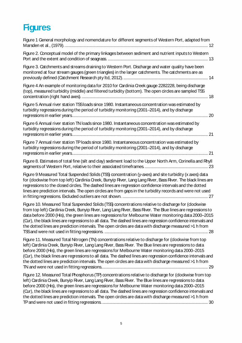
Figures Figure 1 General morphology and nomenclature for different segments of Western Port, adapted from Marsden et al., (1979). ............................................................................................................................... 12

Figure 2. Conceptual model of the primary linkages between sediment and nutrient inputs to Western Port and the extent and condition of seagrass. ......................................................................................... 13

Figure 3. Catchments and streams draining to Western Port. Discharge and water quality have been monitored at four stream gauges (green triangles) in the larger catchments. The catchments are as previously defined (Catchment Research pty ltd, 2012). ........................................................................... 14

Figure 4 An example of monitoring data for 2010 for Cardinia Creek gauge 2282228, being discharge (top), measured turbidity (middle) and filtered turbidity (bottom). The open circles are sampled TSS concentration (right hand axes). ................................................................................................................ 18

Figure 5 Annual river station TSS loads since 1980. Instantaneous concentration was estimated by turbidity regressions during the period of turbidity monitoring (2001–2014), and by discharge regressions in earlier years. ........................................................................................................................ 20

Figure 6 Annual river station TN loads since 1980. Instantaneous concentration was estimated by turbidity regressions during the period of turbidity monitoring (2001–2014), and by discharge regressions in earlier years. ........................................................................................................................ 21

Figure 7 Annual river station TP loads since 1980. Instantaneous concentration was estimated by turbidity regressions during the period of turbidity monitoring (2001–2014), and by discharge regressions in earlier years. ........................................................................................................................ 21

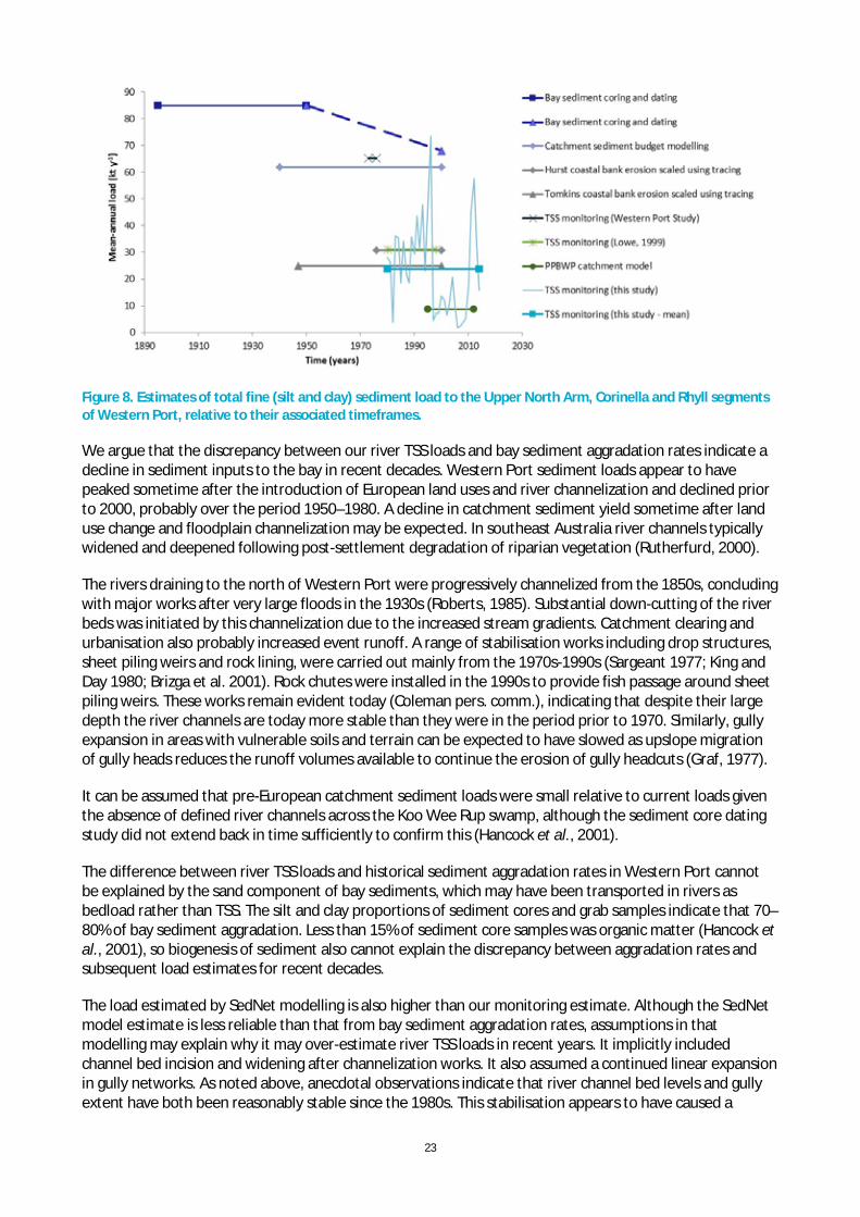
Figure 8. Estimates of total fine (silt and clay) sediment load to the Upper North Arm, Corinella and Rhyll segments of Western Port, relative to their associated timeframes. ........................................................ 23

Figure 9 Measured Total Suspended Solids (TSS) concentration (y-axes) and site turbidity (x axes) data for (clockwise from top left) Cardinia Creek, Bunyip River, Lang Lang River, Bass River. The black lines are regressions to the closed circles. The dashed lines are regression confidence intervals and the dotted lines are prediction intervals. The open circles are from gaps in the turbidity records and were not used in fitting regressions. Excluded outliers are not shown. ............................................................................ 27

Figure 10. Measured Total Suspended Solids (TSS) concentrations relative to discharge for (clockwise from top left) Cardinia Creek, Bunyip River, Lang Lang River, Bass River. The Blue lines are regressions to data before 2000 (His), the green lines are regressions for Melbourne Water monitoring data 2000–2015 (Cur), the black lines are regressions to all data. The dashed lines are regression confidence intervals and the dotted lines are prediction intervals. The open circles are data with discharge measured >1 h from TSS and were not used in fitting regressions. ............................................................................................ 28

Figure 11. Measured Total Nitrogen (TN) concentrations relative to discharge for (clockwise from top left) Cardinia Creek, Bunyip River, Lang Lang River, Bass River. The Blue lines are regressions to data before 2000 (His), the green lines are regressions for Melbourne Water monitoring data 2000–2015 (Cur), the black lines are regressions to all data. The dashed lines are regression confidence intervals and the dotted lines are prediction intervals. The open circles are data with discharge measured >1 h from TN and were not used in fitting regressions............................................................................................... 29

Figure 12. Measured Total Phosphorus (TP) concentrations relative to discharge for (clockwise from top left) Cardinia Creek, Bunyip River, Lang Lang River, Bass River. The Blue lines are regressions to data before 2000 (His), the green lines are regressions for Melbourne Water monitoring data 2000–2015 (Cur), the black lines are regressions to all data. The dashed lines are regression confidence intervals and the dotted lines are prediction intervals. The open circles are data with discharge measured >1 h from TP and were not used in fitting regressions. .............................................................................................. 30

6

Figure 14 Port Bay catchment showing major rivers and creeks. The red triangle shows the name and location of gauging stations and the orange circle represents the location of stream photos shown in the next figure .................................................................................................................................................. 34

Figure 15 River cross sections for a) Cardinia Creek, b) Bunyip River, c) Lang Lang River and d) Bass River, within the floodplain reaches of these streams (locations are shown in Figure 14) ................................. 36

Figure 16 Left: River bank height (left) and width of vegetation (right) for each 100 m section of stream, as assessed for the Index of Stream Condition 2010 (Wilson, 2014). ........................................................ 36

Figure 17 River bed profile of Cardinia Creek based on LiDAR 1m DEM .................................................... 37

Figure 18 Typical example of stream cross-sections: a) single channel 3 km upstream of Cardina, b) multiple channels at Ballarto Road Crossing, 5 km upstream of Gippsland Highway. The values above each plot illustrate how different channel roughness values were applied to the channel and floodplain segments of cross sections. ........................................................................................................................ 37

Figure 19 Cumulative bed material particle size distributions for Western Port rivers ............................. 39

Figure 20 Observed and modelled sediment concentrations relative to stream discharge at Cardinia, based on a daily time series for 2013, and compared with the observed sediment concentrations estimated in Section 2. ............................................................................................................................... 39

Figure 22 Sediment delivery ratio between catchment outlet (4.8 km from river mouth) and Glen Forbes gauge (13 km from the river mouth) for the Bass River. Results presented are based on daily time series of sediment delivery rate in 2011 and 2013. ............................................................................................. 40

Figure 23 Sediment delivery ratio to estimate catchment sediment delivery from the stream gauges to Western Port for the Cardinia, Bunyip, Lang Lang and Bass rivers ............................................................ 41

Figure 24 Erosion and deposition rate as a function of stream discharge for Cardinia Creek ................... 42

Figure 25 Spatial distribution of erosion and deposition along Cardinia Creek. A positive value indicates a sediment source and a negative value indicates sediment sink. Results are based on a simulation period of 1/01/2013 to 31/12/2013. ..................................................................................................................... 42

Figure 26 Spatial distribution of erosion and deposition along the Bunyip River. A positive value indicates a sediment source and a negative value indicates sediment sink. Results are based on a simulation period of 1/01/2013 to 31/12/2013. .......................................................................................................... 43

Figure 27 Spatial distribution of erosion and deposition along the Lang Lang River. A positive value indicates a sediment source and a negative value indicates sediment sink. Results are based on a simulation period of 1/01/2013 to 31/12/2013. ........................................................................................ 43

Figure 28 Spatial distribution of erosion and deposition along the Bass River. A positive value indicates a sediment source and a negative value indicates sediment sink. Results are based on a simulation period of 1/01/2013 to 31/12/2013. ..................................................................................................................... 43

Figure 29 Average coastal bank erosion rates over the period prior to each monitoring date. A linear regression is fitted to the data. .................................................................................................................. 46

Figure 30 (Left) Average coastal bank erosion rates at each monitoring profile over 33 months to August 2015. (Right) Location of each erosion pin profile (Tag) at the site, reproduced from (Tomkins et al., 2014). .......................................................................................................................................................... 46

Figure 31. Webcam images near the start and end of monitoring illustrate the coastal erosion over the monitoring period. The top image is from 10 November 2012, 17:45pm; the bottom image is from 8 February 2016, 6:00pm. The dark blue vertical lines connect features identical to both images (shrub in centre, erosion pin at right). The light blue vertical lines indicate erosion over the 39 months between the two images of (from left) the lower and upper bank face at the headland, and lower and upper bank face in the crenulation/inlet. ...................................................................................................................... 47

7

Figure 32 Left: Coastal bank erosion monitoring site at 11:45 am on 24 June 2014. Right: the site on 26 November 2014. ......................................................................................................................................... 48

Figure 33 Left: Vegetation density affected by wave inundation behind the crenulation section. Right: Looking downwards showing tension cracks running along the top of the lower bank adjacent to the headland at the southern end of the site. .................................................................................................. 48

Figure 34 Coastal bank erosion site during high tide, 9 October 2012. ..................................................... 49

Figure 35: The SAMBUCA physics-based approach using atmospherically corrected imagery (in rrs) and an objective process of quality control. The 3 steps include an image noise estimate, inversion optimisation (SAMBUCA), and finally a quality control step. Optimally, a bathymetry layer is used to constrain Step 2. ................................................................................................................................................................. 53

Figure 36: Western Port bathymetry from LiDAR and acoustic measurements (source: Melbourne Water). ........................................................................................................................................................ 55

Figure 37: Averaged specific inherent optical properties (SIOPs) used in the optical model. Data was acquired from field and laboratory measurements. .................................................................................. 55

Figure 38: The solid lines show in situ reflectance spectra, collected with a RAMSES spectrometer over a seagrass (Zostera spp.) and brown macroalgae (Cockleweed), green and brown solid lines respectively. Long dashed lines show surface reflectance spectra modelled to the Landsat 5 spectral bands and the dotted lines show the Landsat 8 modelled reflectance. The placement and bandwidth of the Landsat 5 TM and Landsat 8 spectral bands are indicated. ........................................................................................ 57

Figure 39. Spectral characteristics of Landsat TM/ETM+ (top) and Landsat 8 (lower) overlaid on 4 common seagrass species spectra found in Western Port Bay. ................................................................. 58

Figure 40. Seagrass map derived from Stephens (1995). ........................................................................... 59

Figure 41. Seagrass map derived from Blake and Ball (2001) .................................................................... 60

Figure 42: Site locations of Landsat water quality time-series which were compared with the EPA sites 709 (Hastings), 716 (Barrallier) and 724 (Corinella). .................................................................................. 60

Figure 43 Classification of the Landsat MSS image from 19 January 1973. This classification was labelled using Bulthuis, 1974. .................................................................................................................................. 61

Figure 44 Classification of the Landsat MSS image from 19 March 1979. This classification was labelled comparing the Bulthuis, 1974 map. Diagonal lines in the classification are coherent noise. .................... 62

Figure 45 Macrophyte cover retrieved from the Landsat 5 TM data acquired 11 April 1988. .................. 63

Figure 46 Macrophyte cover retrieved from the Landsat 5 TM data acquired 29 December 1990. ......... 64

Figure 47 Macrophyte cover retrieved from the Landsat 5 TM data acquired 21 October 1994. ............. 64

Figure 48 Macrophyte cover retrieved from the Landsat 5 TM data acquired 31 October 1998. ............. 65

Figure 49: The Landsat 5 image of Western Port Bay from 10 April 1999 with the retrieved bare, macroalgae, seagrass and combined seagrass/macroalgae classes in light blue, green, red and dark blue, respectively. ................................................................................................................................................ 65

Figure 50: The Landsat 5 image of Western Port Bay from 2 February 2001 with the retrieved bare, seagrass, algae and combined seagrass/macroalgae classes in light blue, red, green and dark blue, respectively. ................................................................................................................................................ 66

Figure 51: The Landsat 5 image of Western Port Bay from 18 January 2004 with the retrieved bare, seagrass, algae and combined seagrass/macroalgae classes. .................................................................... 66

Figure 52: The Landsat 5 image of Western Port Bay from 27 August 2009 with the retrieved seagrass, algae and bare substrate classes. ............................................................................................................... 67

8

Figure 53 : The Landsat 8 image of Western Port Bay from 26 August 2014 with the retrieved seagrass and algae classes. ....................................................................................................................................... 67

Figure 54: The areal extent of benthic cover estimated by SAMBUCA from the Landsat time series (at various tidal states). Data labels are the total area assessed at each date in square kilometres. A maximum likelihood classification was used for the 1973 and 1979 data and the SAMBUCA method was used for subsequent years. The ‘seagrass’, ‘macroalgae’, and ‘seagrass &/or macroalgae’ classes were combined. ................................................................................................................................................... 68

Figure 55: Monthly river TSS loads summed across the four stream gauges (from Section 2.3.2) compared with the time series of non-algal particulate concentrations from Landsat SAMBUCA modelling in the Corinella segment of Western Port. ................................................................................ 72

Figure 56. Maps of non-algal particulate (NAP) concentration from the SAMBUCA model, based on the same Landsat 5, 7 & 8 images for which seagrass and macro-algae were predicted (from 11 April 1988 top left until 26 August 2014, bottom right). Higher concentrations are shown in blue, intermediate concentrations in green and lower concentrations in red. The historical tide height estimates were obtained using WXTide32 (http://www.wxtide32.com/index.html), developed by the National Ocean Service (U.S.A.), and are not validated. ...................................................................................................... 75

Figure 57: SAMBUCA retrieval of non-algal particulates (NAP) concentration from the USGS images (circles), and from the AGDC (triangles) in the Corinella segment, compared with TSS measurements at the EPA Corinella site (squares).................................................................................................................. 76

Figure 58: SAMBUCA retrieval of non-algal particulates (NAP) concentration from the USGS images (circles), and from the AGDC (triangles) in the Upper North Arm, compared with TSS measurements at the EPA Barrallier Island site. ..................................................................................................................... 76

Figure 59: SAMBUCA retrieval of non-algal particulates (NAP) concentration in the Lower North Arm segment from the USGS images (circles), compared with TSS measurements at the EPA Hastings site (squares). No AGDC retrievals were undertaken for this site. ................................................................... 76

Figure 60: The comparison between the surface reflectance products produced by the AGDC (y-axis) and the USGS (x-axis) for the blue, green and red bands. ................................................................................ 77

Figure 61: The SAMBUCA retrieved Kd (490nm) from USGS data (circles) compared with the EPA Kd (squares) as calculated from PAR measurements at the EPA Corinella sampling location (EPA measurements from Holland et al., 2013). ................................................................................................ 78

Figure 62: The SAMBUCA retrieved Kd (490nm) from USGS data (circles) compared with the EPA Kd (squares) as calculated from PAR measurements at the EPA Barrallier Island sampling location (EPA measurements from Holland et al., 2013). ................................................................................................ 78

Figure 63: The SAMBUCA retrieved Kd (490nm) from USGS data (circles) compared with the EPA Kd (squares) as calculated from PAR measurements at the EPA Hastings sampling location (EPA measurements from Holland et al., 2013). ................................................................................................ 78

Figure 64: The SAMBUCA retrievals for Kd (490 nm) from the USGS Landsat 5, 7 & 8 images acquired from 11 April 1988 top left until 26 August 2014, bottom right. Low Kd (490nm) values (shown in red) indicating increased water clarity and light availability at the seafloor. .................................................... 79

Figure 65: MODIS Aqua mean values for Kd 490 nm (grey) from whole of the Western Port Bay area from July 2002 until September 2015 within the region specified by the polygon, top left:38.20°S,145.11°E and lower right 38.53°S, 145.57°E. This data is available in a tabular format with geographic reference and date. The MODIS data is compared with the Landsat SAMBUCA retrieved Kd (490nm) as circles compared with the EPA Kd as squares as calculated from PAR measurements at the EPA Hastings sampling location (EPA measurements from Holland et al., 2013). ..................................... 80

Figure 66: MODIS Aqua K_490 1km monthly time series for Australia, Dataset ID: csiro_1m_1km_aust_K_490. ...................................................................................................................... 82

9

Figure 67: A Landsat 8 image acquired on 25 April 2016 at very low tide. Significant macrophyte coverage is exposed on the intertidal flats and substrate visibility is possible in the majority of the bay. Although SAMBUCA would not be able to retrieve the emergent macrophytes, a standard spectral classification method would potentially be able to discriminate the substrate at a higher resolution. ... 84

Figure 68. Seagrass simulation for increasing sea level with 1 m per 100 years (red). Black line: reference simulation. Straight and broken line in the upper panel refer to biomass of shoot and root, respectively. ................................................................................................................................................ 95

Figure 69. Seagrass simulation for increasing water temperature with 4 C per 100 years (red). Black line: reference simulation. Straight and broken line in the upper panel refer to biomass of shoot and root, respectively. ................................................................................................................................................ 96

Figure 70. Simulated shoot biomass for different values of absorption at a depth of H = 1 m. ................ 97

Figure 71. Simulated shoot biomass for different values of depth at absorption of kd = 0.5 1/m............. 97

Figure 72. Seagrass distribution determined from Landsat satellite imagery for 1994, colour coded with bathymetric depth of occurrence. .............................................................................................................. 98

Figure 73. Simulated seagrass distribution colour coded for shoot biomass. ........................................... 98

Figure 74. Simulated seagrass distribution colour coded for shoot density. ............................................. 99

10

Tables Table 1 Extent of monitoring data from the Melbourne Water Loads Monitoring Program used to estimate turbidity-based load time-series ................................................................................................. 18

Table 2 Scaling of mean-annual TSS, TN and TP loads to estimate basin exports to Western Port (1980—2014). .......................................................................................................................................................... 22

Table 3 Bulk density of bed material across each river .............................................................................. 38

Table 4 Clay component (particle size < 4µm) of bed material in each river ............................................. 38

Table 5: Symbols and definitions of parameters use in the SAMBUCA model .......................................... 52

Table 6: Landsat imagery acquired from the USGS Earth Explorer site (row/path = 092/087; http://earthexplorer.usgs.gov/ ). ............................................................................................................... 54

Table 7. Collation of water quality information ......................................................................................... 56

Table 8: Parameterisation used in optical model for Western Port Bay imagery ...................................... 56

Table 9. Habitat baseline data and maps ................................................................................................... 59

Table 10: The pixel accuracy assessment of the 1994 Landsat SAMBUCA retrieved substrates when compare with the Stephens (1995) field data collected during 1994. The overall accuracy is low at 10%, kappa co-efficient of -0.0163. .................................................................................................................... 70

Table 11: The pixel accuracy assessment of the 1994 Landsat SAMBUCA retrieved substrates when compare with the combined algae and seagrass classes from the Stephens (1995) field data collected during 1994. The overall accuracy is 65%, with a kappa coefficient at 0.0092. ......................................... 70

Table 12: The pixel accuracy assessment of the 1998 Landsat SAMBUCA retrieved substrates when compare with the Blake and Ball (2001) field data collected during 1999. The overall accuracy is low at 52%, kappa co-efficient of 0.0384. ............................................................................................................. 70

Table 13: The pixel accuracy assessment of the 1998 Landsat SAMBUCA retrieved substrates when compare with the combined algae and seagrass classes from the Blake and Ball (2001) field data collected during 1999. The overall accuracy is 85%, with a kappa coefficient at 0.0199. ......................... 71

Table 14: The pixel accuracy assessment of the 1999 Landsat SAMBUCA retrieved substrates when compare with the Blake and Ball (2001) field data collected during 1999. The overall accuracy is low at 16%, kappa co-efficient of 0.0121. ............................................................................................................. 71

Table 15: The pixel accuracy assessment of the 1999 Landsat SAMBUCA retrieved substrates when compare with the combined algae and seagrass classes from the Blake and Ball (2001) field data collected during 1999. The overall accuracy is 95%, with a kappa coefficient at 0.752. ........................... 71

11

Acknowledgments

This research was funded by Melbourne Water and CSIRO. Technical assistance with fieldwork was provided by Gordon McLachlan (CSIRO). Steve Marvanek extracted cross sections from the LiDAR DEM for Section 3. Drafts of the report were reviewed by Hannalie Botha, Jenny Skerratt and Nick Potter (CSIRO).

12

1 Introduction

1.1 State and drivers of bay turbidity and seagrass

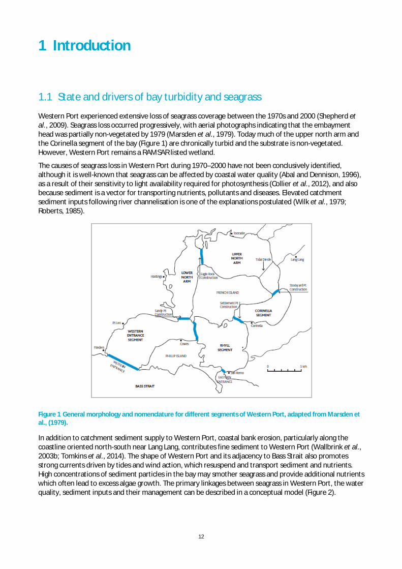
Western Port experienced extensive loss of seagrass coverage between the 1970s and 2000 (Shepherd et al., 2009). Seagrass loss occurred progressively, with aerial photographs indicating that the embayment head was partially non-vegetated by 1979 (Marsden et al., 1979). Today much of the upper north arm and the Corinella segment of the bay (Figure 1) are chronically turbid and the substrate is non-vegetated. However, Western Port remains a RAMSAR listed wetland.

The causes of seagrass loss in Western Port during 1970–2000 have not been conclusively identified, although it is well-known that seagrass can be affected by coastal water quality (Abal and Dennison, 1996), as a result of their sensitivity to light availability required for photosynthesis (Collier et al., 2012), and also because sediment is a vector for transporting nutrients, pollutants and diseases. Elevated catchment sediment inputs following river channelisation is one of the explanations postulated (Wilk et al., 1979; Roberts, 1985).

Figure 1 General morphology and nomenclature for different segments of Western Port, adapted from Marsden et al., (1979).

In addition to catchment sediment supply to Western Port, coastal bank erosion, particularly along the coastline oriented north-south near Lang Lang, contributes fine sediment to Western Port (Wallbrink et al., 2003b; Tomkins et al., 2014). The shape of Western Port and its adjacency to Bass Strait also promotes strong currents driven by tides and wind action, which resuspend and transport sediment and nutrients. High concentrations of sediment particles in the bay may smother seagrass and provide additional nutrients which often lead to excess algae growth. The primary linkages between seagrass in Western Port, the water quality, sediment inputs and their management can be described in a conceptual model (Figure 2).

13

Figure 2. Conceptual model of the primary linkages between sediment and nutrient inputs to Western Port and the extent and condition of seagrass.

Beyond defining the inputs and their links to seagrass, establishing the connections to the ecosystem health of the bay can be complicated by significant delays in response (Meals et al., 2010). For example, there are several components which would delay water quality improvement in Western Port following catchment and streambank erosion management:

1. The time of vegetation response, e.g. establishment of new plant communities. Typically the effectiveness of trees at mitigating bank erosion is by root reinforcement of soil, and their effect in modulating soil moisture. The former effect increases with their rooting density and depth (Abernethy and Rutherfurd, 2001), meaning that it could take decades between tree planting and when they reach full effectiveness. Implementing revegetation at scale also takes time.

2. The time for that vegetation to modify erosion processes. Once vegetation is effective, a range of runoff event sizes must be experienced to provide the opportunity for erosion to be modified.

3. The time required to detect a change in river water quality. A range of conditions must also be experienced to detect a significant change in river TSS loads. For example, it has been estimated that the existing comprehensive TSS monitoring program in the Burdekin River in Queensland will require 20 years to detect a 15% change in annual TSS load at a 90% confidence level (Darnell et al., 2012).

4. The time for the water body to respond to the effect, due to sediment residence times or the time required for a range of hydrologic conditions to occur within Western Port. The degree to which bay turbidity responds to ongoing sediment and nutrient inputs from catchment runoff events, and the timing of such responses are not known. Sediment transport within Western Port is predominantly from the ocean entrances landward (Harris et al., 1979), such that sediment delivered to the bay is predominantly stored within the bay (Hancock et al., 2001), rather than being exported in tidal outflows. There is a slow clockwise movement around French Island in accordance to wind/wave and tidal forcing. Tidal resuspension causes TSS concentrations up to several grams per litre near Lang Lang (Tomkins et al., 2014). Consequently, this resuspended ‘internal load’ may be more significant than river inputs at least under ambient catchment conditions. However, river inflows can play a dominant role in coastal water quality. For example,

River sediment and nutrient inputs Coastal bank erosion

Western Port benthic light climate

Seagrass extent and condition

Resuspension by tides and waves

Sediment redistribution

Flood plumes

Colonisation, Mortality

Seagrass growth rate

Surface runoff Gully erosionStream bank erosion

VegetationRunoff controls

Epiphyte growth

Smothering

Aggradation

Internal nutrient load

Sediment storage

14

water clarity off-shore the Burdekin River has been observed to progressively recover over several months following large river flows of turbid water (Fabricius et al., 2014).

1.2 Catchment management and water quality responses

Western Port is a key value within Melbourne Water’s Healthy Waterways and Stormwater strategies (Melbourne Water 2013a; 2013b), and therefore, Melbourne Water undertakes catchment and waterway management activities, including riparian fencing and revegetation, urban and rural stormwater management, and stream bed and bank stabilisation to protect and improve the health of the bay. Given that streambank erosion is the largest sediment source, controlling stock access to streams and riparian revegetation are key actions. Revegetating river banks can increase erosion resistance during floods relative to non-vegetated river banks exposed to comparable stream power (Hardie et al., 2012).

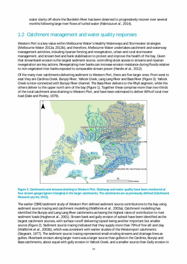
Of the many river catchments delivering sediment to Western Port, there are five larger ones. From west to east they are Cardinia Creek, Bunyip River, Yallock Creek, Lang Lang River and Bass River (Figure 3). Yallock Creek is inter-connected with Bunyip River channel. The Bass River delivers to the Rhyll segment, while the others deliver to the upper north arm of the bay (Figure 1). Together these comprise more than two-thirds of the total catchment area draining to Western Port, and have been estimated to deliver 80% of total river load (Dale and Pooley, 1979).

Figure 3. Catchments and streams draining to Western Port. Discharge and water quality have been monitored at four stream gauges (green triangles) in the larger catchments. The catchments are as previously defined (Catchment Research pty ltd, 2012).

The earlier CSIRO sediment study of Western Port defined sediment source contributions to the bay using sediment source tracing and catchment modelling (Wallbrink et al., 2003a). Catchment modelling has identified the Bunyip and Lang Lang River catchments as having the highest rates of contribution to river sediment loads (Hughes et al., 2001). Stream bank and gully erosion of subsoil have been identified as the largest catchment sources, with surface runoff delivering topsoil being another important but smaller source (Figure 2). Sediment source tracing indicated that they supply more than 79% of fine silt and clay (Wallbrink et al., 2003b), which was consistent with earlier studies of the Westernport catchments (Sargeant, 1977). The sediment source tracing represented small eroding streams and drainage lines as gullies. Riverbank erosion along larger rivers was a larger source than gullies in the Cardinia, Bunyip and Bass catchments, about equal with gully erosion in Yallock Creek, and a smaller source than Gully erosion in

15

the Lang Lang catchment (Wallbrink et al., 2003b). Consequently, several studies have identified riparian revegetation as a priority action to reduce river sediment loads.

Extensive channelization of rivers through the large Koo Wee Rup swamp, for flood mitigation, has also increased the efficiency with which sediment from catchment erosion is delivered to the coast. Channelization works commenced in the 1870s in the Cardinia catchment, expanded in the 1890s, and continued until the 1950s. The formed channels can be sediment sources themselves, particularly around the upstream margins of the former floodplain. Significant sediment removal is also undertaken to maintain the size of the channels, indicating deposition in some areas and under most flow conditions. SedNet modelling also found that lower reaches of these streams were predicted to experience sand and gravel deposition (Hughes et al., 2003).

1.3 Research scope

The Western Port science review, Understanding the Western Port environment: a summary of current knowledge and priorities for future research (Melbourne Water 2013) emphasised the importance of developing a systems understanding of Western Port. The conceptual model above is a high-level contribution towards that goal. Our research activities focused on four aspects of the linkages between river sediment and nutrient loads and Western Port turbidity, and seagrass extent and growth:

1. Available river station monitoring data were used to reconstruct historical time-series of fine sediment, nitrogen and phosphorus loads from rivers draining to Western Port, to assess historical changes including by comparison with earlier load estimates (Sections 2 and 3 of this report). An ancillary aim was to improve knowledge of catchment sediment contributions to guide priorities for catchment management.

2. Monitoring of coastal bank erosion rates was extended from 13 months in a preceding project out to 3.5 years, to assess the contribution to Western Port sediment loads (Section 4 of this report). Together activities 1 and 2 address consolidated research needs identified in the Western Port Environmental Research Review (Melbourne Water 2011):

o #4 “Measure residence time of sediments entering the bay, by determining temporal changes in sediment and sediment associated nutrient inputs to the bay over time.”

o #6 “Estimate contribution of coastal erosion to nutrient and sediment budgets” o #12 “Determine preliminary nutrient (N & P) budget, at the scale of the five

basins/segments” in Western Port. 3. Spectral analysis techniques were applied to remote sensing imagery of the bay to investigate its

capability to represent historical turbidity levels and seagrass extent, to extrapolate spatially from in situ measurements, and for future routine monitoring of seagrass extent and water clarity (Section 5 of this report). We also investigated the existence of linkages between catchment inputs and remotely-sensed bay turbidity. This addressed consolidated research needs identified in the Western Port Environmental Research Review (Melbourne Water 2011):

o #16 “Determine water quality targets for sediments and nutrients that support seagrasses” 4. Conceptual modelling was undertaken of the primary drivers of seagrass growth and feedbacks

between bay light climate, sediment inputs, sediment resuspension and seagrass growth to underpin spatial modelling of seagrass (Section 6 of this report). This assisted Melbourne Water to develop a hydrodynamic, wave and biogeochemical model of the bay. This activity also addressed consolidated research needs identified in the Western Port Environmental Research Review (Melbourne Water 2011):

o #5 “Refine understanding of effects of seagrass on sediment transport” o #15 “Assess the degree of nutrient and light limitation of major primary producers” o #16 “Determine water quality targets for sediments and nutrients that support seagrasses”

16

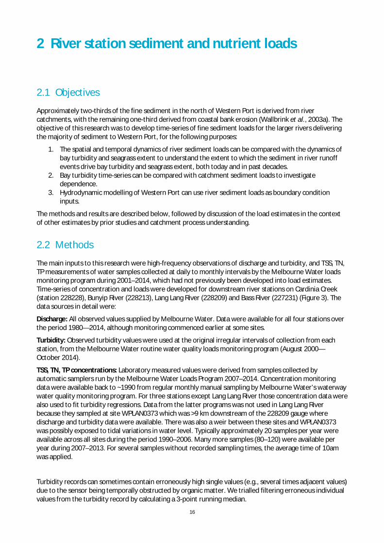
2 River station sediment and nutrient loads

2.1 Objectives

Approximately two-thirds of the fine sediment in the north of Western Port is derived from river catchments, with the remaining one-third derived from coastal bank erosion (Wallbrink et al., 2003a). The objective of this research was to develop time-series of fine sediment loads for the larger rivers delivering the majority of sediment to Western Port, for the following purposes:

1. The spatial and temporal dynamics of river sediment loads can be compared with the dynamics of bay turbidity and seagrass extent to understand the extent to which the sediment in river runoff events drive bay turbidity and seagrass extent, both today and in past decades.

2. Bay turbidity time-series can be compared with catchment sediment loads to investigate dependence.

3. Hydrodynamic modelling of Western Port can use river sediment loads as boundary condition inputs.

The methods and results are described below, followed by discussion of the load estimates in the context of other estimates by prior studies and catchment process understanding.

2.2 Methods

The main inputs to this research were high-frequency observations of discharge and turbidity, and TSS, TN, TP measurements of water samples collected at daily to monthly intervals by the Melbourne Water loads monitoring program during 2001–2014, which had not previously been developed into load estimates. Time-series of concentration and loads were developed for downstream river stations on Cardinia Creek (station 228228), Bunyip River (228213), Lang Lang River (228209) and Bass River (227231) (Figure 3). The data sources in detail were:

Discharge: All observed values supplied by Melbourne Water. Data were available for all four stations over the period 1980—2014, although monitoring commenced earlier at some sites.

Turbidity: Observed turbidity values were used at the original irregular intervals of collection from each station, from the Melbourne Water routine water quality loads monitoring program (August 2000—October 2014).

TSS, TN, TP concentrations: Laboratory measured values were derived from samples collected by automatic samplers run by the Melbourne Water Loads Program 2007–2014. Concentration monitoring data were available back to ~1990 from regular monthly manual sampling by Melbourne Water’s waterway water quality monitoring program. For three stations except Lang Lang River those concentration data were also used to fit turbidity regressions. Data from the latter programs was not used in Lang Lang River because they sampled at site WPLAN0373 which was >9 km downstream of the 228209 gauge where discharge and turbidity data were available. There was also a weir between these sites and WPLAN0373 was possibly exposed to tidal variations in water level. Typically approximately 20 samples per year were available across all sites during the period 1990–2006. Many more samples (80–120) were available per year during 2007–2013. For several samples without recorded sampling times, the average time of 10am was applied.

Turbidity records can sometimes contain erroneously high single values (e.g., several times adjacent values) due to the sensor being temporally obstructed by organic matter. We trialled filtering erroneous individual values from the turbidity record by calculating a 3-point running median.

17

The rapid variations in TSS, TN, TP concentration during runoff events were represented using site-specific linear regression relationships between the measured concentrations of water samples, and the turbidity recorded at the stream gauge closest to the time each sample was collected. Dependence between TSS and turbidity was expected (Gippel, 1995). Similar dependence was expected for TN and TP given that significant proportions are transported attached to fine sediment particles, however somewhat poorer explanatory power may be expected because dissolved concentrations are independent of turbidity. Where necessary to linearise the response, turbidity was square-root or log10 transformed before fitting the regression.

TSS, TN and TP concentration regressions were also fitted against discharge. Discharge was square root or log10 transformed to linearise the response. Separate regressions were fitted for the periods prior to the start of turbidity monitoring at each gauge, and subsequent to that time for comparison with turbidity-based concentration estimates and to estimate concentration after the conclusion of turbidity monitoring.

Concentration measurements whose sampling times differed by more than one hour from those of the adjacent turbidity (or discharge) measurements were not used in fitting regressions. This process excluded ~20% of data points, but improved the regression R2 values. Trialling a 15 minute data gap resulted in almost identical regressions but lower R2 values due to the fewer points available.

Data points >2 times the 95% prediction interval from each regression (i.e., >4 standard deviations) were excluded as outliers and the regressions were refitted. Only a few data points were defined as outliers, generally high concentration at low turbidity or discharge.

The TSS, TN, TP concentrations were then calculated for each turbidity observation (or discharge observation for discharge regressions) using the regressions. To calculate loads for each monitoring interval, discharge and concentration were linearly interpolated between observations (the trapezoid method), so long intervals did not automatically bias load estimation even though they increased uncertainty. Load was calculated in SI units for each period as the product of mean discharge and concentration. In a small number of cases where the regression had a negative intercept, negative predicted values were replaced with zero. These negative intercepts were small and not statistically significant. The regression confidence intervals were used to calculate upper and lower bounds of concentration and load.

2.3 Results

2.3.1 CONCENTRATION DATA CHARACTERISTICS

The turbidity monitoring duration extended for ~15 years at 3 sites, and ~8 years at 1 site (Table 1). Longer intervals between discharge measurements were evident during drier periods which did not overly affect the quality of load estimates. The intervals of water sampling for TSS concentration were generally constant (Figure 4). Most elevated concentrations and turbidity coincided with elevated discharge as expected. There was little measurement noise generally apparent in the turbidity time-series, with the exception of station 228228, which had more variable turbidity during event periods. The filtering of turbidity data had the effect of flattening the amplitude of variations and did not exclude a significant number of outliers, so the original turbidity data were adopted for fitting TSS regressions and for load estimation.

18

Table 1 Extent of monitoring data from the Melbourne Water Loads Monitoring Program used to estimate turbidity-based load time-series

RIVER STATION START DATE END DATE TURBIDITY (N) TSS (N) TN (N) TP (N)

Cardinia Creek 228228A 16/08/2000 20/10/2014 361,426 231 191 191

Bunyip River 228213 16/08/2000 20/10/2014 291,244 227 174 174

Lang Lang River 228209B 16/08/2000 20/10/2014 291,092 58 52 52

Bass River 227231 21/12/2006 17/03/2014 225,212 206 183 183 A TSS, TN, TP data collected at WPCAR0133 site (4.5 km downstream of 228228) B At 228209 TSS, TN, TP data was available for fitting regressions against turbidity only from 2007 onwards, because monitoring for the period 2000–2007 occurred only at WPLAN0373 site (9 km downstream).

Figure 4 An example of monitoring data for 2010 for Cardinia Creek gauge 2282228, being discharge (top), measured turbidity (middle) and filtered turbidity (bottom). The open circles are sampled TSS concentration (right hand axes).

The majority of data points were at low turbidity (Figure 9). This may be a consequence of the sample analysed from each event being randomly selected. There was considerable scatter around the TSS-turbidity relationships. In the absence of detailed knowledge of the monitoring sites and equipment it is difficult to identify causes of the scatter. Variations in particle size distributions are a possibility, although one which has been previously found to provide little improvement in the explained variance (Gippel, 1995). Organic contamination of the turbidity sensor or TSS intake is another possibility, although the turbidity sensors had automatic wiper devices for cleaning. Another possibility is local sources of turbidity unrelated to runoff such as stock access to streams or dry weather discharges into urban drainage systems.

Because TSS load increases in proportion with concentration and discharge, for estimating sediment loads, “the most important feature of the relationship is not necessarily its percentage explained variance, but its

19

ability to predict the high concentration values” (Gippel, 1995). On this aspect the regressions performed reasonably, being in the middle of the observed range of TSS values at high turbidity (Figure 9; in Section 2.6.1).

The event focus of monitoring during 2007–2013 resulted in poorer fits for TSS regressions against discharge relative to those for the period up to 2000, in all streams (see Section 2.6.1). However, TSS, TN and TP concentrations were much better explained by turbidity than by discharge for the period since 2001, and the selected regressions had sufficiently high R2 values for robust load estimation (see supplementary data Section 2.6). Extrapolation of regressions to higher observed values of turbidity or discharge did not appear to result in unrealistically high concentrations, because constraining concentrations to be always less than the maximum observed values resulted in mean-annual load estimates within 3% of those with unconstrained concentrations.

Temporal changes in concentration regressions

Comparing TSS concentrations during 2001–2014 with those in the 1990s, in most cases, the confidence intervals of regressions against discharge for the two periods overlap, indicating no significant change. However, there were several significant changes in measured TSS, TN or TP concentrations in the four streams:

· Bunyip River TSS concentrations have increased at small discharges <10 m3 s-1 (Figure 10; in Section 2.6.1). This type of change is likely to be caused by local and/or chronic sources (Norris et al., 2007; Wilkinson, 2012). Plausible but untested causes of this nature include an increase in livestock access to streams (unlikely), or earthworks (e.g., road and residential construction). Pockets of urban growth occurred since 2001 in Garfield, Bunyip and Longwarry.

· Cardinia Ck and Bunyip River TN concentrations have increased. In Bunyip River this occurred over all but very low discharges while in Cardinia Ck the difference was over middle discharges only where there were sufficient data available from the 1990s (Figure 11; in Section 2.6.1). This type of change is likely to be caused by non-point sources affected by event runoff in the upstream catchment (Norris et al., 2007; Wilkinson, 2012). Plausible but untested causes of this nature include increases in the extent of urban land use.

· Bass River TN concentrations have significantly declined at higher discharges (Figure 11; in Section 2.6.1), while TP concentrations have significantly increased at smaller discharges (Figure 12; in Section 2.6.1). The decrease in TN is likely to be caused by non-point sources affected by event runoff in the upstream catchment (Norris et al., 2007; Wilkinson, 2012). Plausible but untested causes of this nature include improved controls on dairy shed effluent. The increase in TP is likely to be associated with local and/or chronic sources (Norris et al., 2007; Wilkinson, 2012). Plausible but untested causes of this nature include an increase in livestock numbers or access to streams associated with increased in fertiliser application rates, or earthworks (e.g., road and residential construction).

· Bunyip River TP concentrations have increased over all but very small discharges (Figure 12; in Section 2.6.1). This type of change is likely to be caused by non-point sources affected by event runoff in the upstream catchment (Norris et al., 2007; Wilkinson, 2012). Plausible but untested causes include an increase in fertiliser application rates or livestock numbers increasing the phosphorus concentration of fine sediment washed into streams.

While possible causes have been noted above, identifying the causes of these changes will require local investigations.

In all streams and constituents the gradients of regression curves are significantly positive, thus these curves can be expected to provide representation of the dynamics of load delivery superior to modelling (such as previous Source model applications) which assume uniform concentration in runoff events regardless of their magnitude.

The proportion of time with discharge and turbidity measurements within 1 week was calculated as a measure of data completeness for calculating load timeseries. Minimum data completeness for any year during the turbidity monitoring period was 86% at 227231 (turbidity gap in 2008), 81% at 228209 (turbidity

20

gap in 2007), 31% at 228213 (discharge gap in 2007) and 75% at 228228 (discharge gap in 2008). These data gaps are unlikely to affect the load estimates considerably because they mainly occurred in very dry years.

To test whether extrapolation of the regressions resulted in unrealistically-large concentrations, the loads were also calculated with maximum limits of concentration applied which were larger than observed within the fitted range of any regression, being TSS 300 mg/L, TN 10 mg/L, TP 1.4 mg/L.

2.3.2 LOAD TIME-SERIES

The sum total of mean-annual TSS loads summed across the 4 river stations for the period 1980–2014 was 17.7 kt yr-1 (95% confidence interval 14.8—20.6) For the period 2001–2014 (the period of the Melbourne Water loads monitoring program), the mean-annual TSS load was somewhat lower at 12.9 kt yr-1 (9.4—16.4) because this period was relatively more affected by the ‘millennium drought’ (1997–2009), when the loads were generally much smaller than in other periods (Figure 5, Figure 6, Figure 7). In contrast, the years 2011 and 2012 had very large loads for the period since 1980, being in the top 3 for TN and TP, and in the top 5 for TSS. The mean-annual TN load since 1980 summed across the 4 river stations was 566 t y-1 (507—624) and the mean-annual TP load was 52.4 t y-1 (45.5—59.3). The Lang Lang River was the largest contributor of TSS and TP load, while Bass and Lang Lang Rivers were approximately equal contributors of TN. Daily load time-series are available as supplementary data.

Figure 5 Annual river station TSS loads since 1980. Instantaneous concentration was estimated by turbidity regressions during the period of turbidity monitoring (2001–2014), and by discharge regressions in earlier years.

21

Figure 6 Annual river station TN loads since 1980. Instantaneous concentration was estimated by turbidity regressions during the period of turbidity monitoring (2001–2014), and by discharge regressions in earlier years.

Figure 7 Annual river station TP loads since 1980. Instantaneous concentration was estimated by turbidity regressions during the period of turbidity monitoring (2001–2014), and by discharge regressions in earlier years.

2.3.3 RIVER EXPORTS TO WESTERN PORT

Mean-annual river TSS export to Western Port is larger than the sum of loads at stream gauges. Only 58% of the area of the four catchments is upstream of the gauges (Figure 3). We used the sediment yields modelled by SedNet at each gauge and river mouth (Hughes et al., 2003) to inform scaling of the gauge

22

loads. This scaling method is better than scaling based on catchment area, because it accounts for the spatial arrangement of erosion and deposition processes relative to gauges, and we have previously used the approach to scale mean-annual loads from gauges to the coast in catchments draining to the Great Barrier Reef lagoon (Kroon et al., 2012). However, it is likely that SedNet over-estimated erosion in the constructed channels downstream of the Cardinia and Bunyip gauges, and it did not represent deposition in these channels. These channels have been enlarged for flood passage, and provide more opportunity for in-channel deposition than do natural channels. Routine manual removal of sediment from these channels indicates net deposition. Thus, we estimated lower scaling ratios in these rivers, to give a total river TSS export to Western Port of 23.8 kt y-1 (Table 2), which was 35% higher than the sum of the loads at river gauges. The river TN and TP loads were also scaled by the same ratios as an estimate of exports to Western Port. Sediment transport modelling (Section 3) offered the possibility of estimating channel sediment delivery including its temporal dynamics, but was not used due to sensitivities in the modelling.

Table 2 Scaling of mean-annual TSS, TN and TP loads to estimate basin exports to Western Port (1980—2014).

CARDINIA BUNYIP LANG LANG BASS SUM

Gauge area (km2) 117 697 272 233

Basin area (km2) 398 1176 423 266 2263

Ratio basin:gauge area 3.40 1.69 1.56 1.14

SedNet ratio export:gauge load 3.56 1.82 1.22 1.11

Estimated ratio export:gauge load 3 1.4 1.22 1.11

Gauge TSS load (kt y-1) 0.95 5.28 7.99 3.48 17.7

Gauge TN load (t y-1) 19.8 152 195 198 566

Gauge TP load (t y-1) 2.49 16.07 21.77 12.07 52.4

Export TSS load (kt y-1) 2.84 7.39 9.71 3.85 23.8

Export TN load (t y-1) 59.4 213 237 219 729

Export TP load (t y-1) 7.47 22.5 26.5 13.3 69.8

Export TSS load (%) 12% 31% 41% 16% 100%

2.4 Discussion

2.4.1 A RECENT DECLINE IN SEDIMENT INPUTS TO WESTERN PORT

The turbidity-based estimates of river export to Western Port presented here can be expected to be more reliable than estimates based on sediment-discharge rating curves alone, and to those based on event mean concentrations. Our mean-annual river TSS load during 1980–2000 is consistent with the estimates of several prior studies specific to recent decades (Figure 8). Load estimates for recent decades have predominantly been lower than estimates of longer-term loads, particularly the input estimated from sediment aggradation in the bay (Figure 8).

23

Figure 8. Estimates of total fine (silt and clay) sediment load to the Upper North Arm, Corinella and Rhyll segments of Western Port, relative to their associated timeframes.

We argue that the discrepancy between our river TSS loads and bay sediment aggradation rates indicate a decline in sediment inputs to the bay in recent decades. Western Port sediment loads appear to have peaked sometime after the introduction of European land uses and river channelization and declined prior to 2000, probably over the period 1950–1980. A decline in catchment sediment yield sometime after land use change and floodplain channelization may be expected. In southeast Australia river channels typically widened and deepened following post-settlement degradation of riparian vegetation (Rutherfurd, 2000).

The rivers draining to the north of Western Port were progressively channelized from the 1850s, concluding with major works after very large floods in the 1930s (Roberts, 1985). Substantial down-cutting of the river beds was initiated by this channelization due to the increased stream gradients. Catchment clearing and urbanisation also probably increased event runoff. A range of stabilisation works including drop structures, sheet piling weirs and rock lining, were carried out mainly from the 1970s-1990s (Sargeant 1977; King and Day 1980; Brizga et al. 2001). Rock chutes were installed in the 1990s to provide fish passage around sheet piling weirs. These works remain evident today (Coleman pers. comm.), indicating that despite their large depth the river channels are today more stable than they were in the period prior to 1970. Similarly, gully expansion in areas with vulnerable soils and terrain can be expected to have slowed as upslope migration of gully heads reduces the runoff volumes available to continue the erosion of gully headcuts (Graf, 1977).

It can be assumed that pre-European catchment sediment loads were small relative to current loads given the absence of defined river channels across the Koo Wee Rup swamp, although the sediment core dating study did not extend back in time sufficiently to confirm this (Hancock et al., 2001).

The difference between river TSS loads and historical sediment aggradation rates in Western Port cannot be explained by the sand component of bay sediments, which may have been transported in rivers as bedload rather than TSS. The silt and clay proportions of sediment cores and grab samples indicate that 70–80% of bay sediment aggradation. Less than 15% of sediment core samples was organic matter (Hancock et al., 2001), so biogenesis of sediment also cannot explain the discrepancy between aggradation rates and subsequent load estimates for recent decades.

The load estimated by SedNet modelling is also higher than our monitoring estimate. Although the SedNet model estimate is less reliable than that from bay sediment aggradation rates, assumptions in that modelling may explain why it may over-estimate river TSS loads in recent years. It implicitly included channel bed incision and widening after channelization works. It also assumed a continued linear expansion in gully networks. As noted above, anecdotal observations indicate that river channel bed levels and gully extent have both been reasonably stable since the 1980s. This stabilisation appears to have caused a

24

reduction in catchment sediment yields since the river channels stabilised after channelization was complete. Therefore, we attached a timeframe of 1940–2000 to this load estimate.

The PPBWP catchment model load estimate is acknowledged as having low confidence (Catchment Research pty ltd, 2012). This model is sensitive to the TSS concentrations, which are typically allocated by landuse class. However, the spatial and temporal variability in concentration within each landuse is large relative to differences between landuses (Waters and Packett, 2007). This variability indicates that variables such as soil type, topography and rainfall intensity have more significant influence on spatial variation in TSS supply than landuse. The derivation of total sediment inputs to Western Port from each of the prior studies is described in Section 2.6.1.

2.4.2 CATCHMENT MANAGEMENT AND POSSIBLE FUTURES FOR WESTERN PORT

Ongoing mud aggradation in the Corinella and Rhyll segments is apparently derived mostly from the North Arm, since the average aggradation rate 1958–2000 was several times larger than the turbidity-based average river inputs 2000–2015. Potentially the decline of seagrass extent in the North Arm contributed to increased sediment remobilisation. It can be hypothesised that bay turbidity and Corinella / Rhyll aggradation rates will decline in future if deposits in the north arm become depleted. Under that scenario the turbidity of Western Port would become more sensitive to ongoing inputs from river catchments and coastal banks.

Priorities for catchment management should reflect the contributions of each catchment to TSS load (Table 2). Our monitoring derived loads indicate that Lang Lang and Bunyip Rivers contribute similar proportions of TSS as previously estimated by SedNet modelling and source tracing. Our load estimates indicate that Bass River contributes a larger proportion of catchment TSS load to the bay (16%) than previously estimated by SedNet modelling (10%) and sediment source tracing (5%). Due to the ungauged area downstream of the gauge site, Cardinia Creek catchment makes more than double the TSS contribution to Western Port (12%) than the 5% indicated by the load at the gauge; this is consistent with SedNet modelling which previously estimated 10%, but less than source tracing which estimated 29% contribution from this catchment.

River rehabilitation activities since 2000 have not yet had an apparent effect on TSS concentrations, or if they have their effects are being counteracted by other changes in supply in the catchments. TSS concentrations in Cardinia Ck Lang Lang River and Bass Rivers have not declined since the 1990s. TSS concentrations in Bunyip River and possibly Cardinia Creek have increased at lower discharges.

2.5 Recommendations

Catchment actions should continue to focus on preventing stock access to streams, managing stream side vegetation and stormwater runoff. Controlling sediment runoff during urban construction is important where that occurs. The Bass River catchment supplies somewhat more TSS than previously estimated, but does not discharge to the primary area of seagrass loss.

To help inform catchment management priorities across Western Port catchments in terms of effectively targeting dominant sediment sources, and identify the nature of effective actions, we recommend working towards a sediment and nutrient budget model representing supply and transport processes. Such a model should be supported by mapping erosion processes throughout drainage networks, particularly gully erosion, streambank stability and vegetation, and risk of pollution from urban and agricultural stormwater runoff.

Future monitoring of river sediment and nutrient loads will help to calibrate catchment load modelling and evaluate catchment management. It is recommended that load monitoring is based on turbidity sensors reporting at 10—20 minute intervals, at least during elevated discharge, to represent the temporal variations within runoff events. This is because turbidity better represents changes in concentration than

25

does discharge (see Section 2.3.1). Details of procedures and suitable types of instrumentation are described by Hawdon et al. (2009), and can be tailored for individual sites. For example, the event water samples selected for laboratory analysis should cover the range of flow and turbidity conditions sampled, to best represent the variation of TSS, TN and TP across the observed range of turbidity and flow. This approach could reduce the width of confidence intervals for regressions for TSS, TN and TP against turbidity at high turbidity levels (Figure 9). Under that approach, flow-weighted event mean concentration could be robustly estimated from the turbidity record if required, rather than directly from irregular water samples. Because regressions between turbidity and pollutant concentrations can vary between turbidity sensors, it is recommended to record the sensor serial number or other unique identifier alongside the data to enable separate regressions to be constructed if a record includes data from multiple turbidity sensors.

Further monitoring could also include analysis of the particle size distributions of TSS in each river to understand its contribution to bay turbidity, noting that the small area and sediment transport conditions in northern Western Port mobilise a range of particle sizes.

26

2.6 Supplementary data on river station loads

2.6.1 REGRESSIONS FOR LOAD ESTIMATION

Properties of the regressions with the best fit to the data which were selected to estimate load time-series for defined periods, being during turbidity monitoring (Turbidity), prior to turbidity monitoring (His) and during and after turbidity monitoring (Cur).

Site Parameter Period Independent variable

Independent variable transformation

Intercept Slope adjR2

227231 TSS Turbidity Turbidity Linear 0 1.084965 0.85866

227231 TN Turbidity Turbidity Square root 1.311232 0.190983 0.139981

227231 TP Turbidity Turbidity Linear 0.118671 0.001955 0.532728

228209 TSS Turbidity Turbidity Linear 38.83492 0.799467 0.191417

228209 TN Turbidity Turbidity Square root 1.374294 0.223729 0.298782

228209 TP Turbidity Turbidity Square root 0.092623 0.034387 0.371908

228213 TSS Turbidity Turbidity Linear 6.607045 0.695481 0.503862

228213 TN Turbidity Turbidity Linear 0.575689 0.024807 0.474726

228213 TP Turbidity Turbidity Linear 0.012977 0.003377 0.63912

228228 TSS Turbidity Turbidity Linear 3.259083 0.577094 0.466882

228228 TN Turbidity Turbidity Square root -0.04733 0.195821 0.603615

228228 TP Turbidity Turbidity Linear 0.036595 0.001272 0.537293

227231 TSS His Discharge Square root -1.51649 21.81439 0.631641

227231 TSS Cur Discharge Square root 1.919831 14.65365 0.459758

227231 TN His Discharge Square root 0.97221 1.02189 0.619872

227231 TN Cur Discharge Square root 1.3945 0.538665 0.447843

227231 TP His Discharge Square root 0.084285 0.045695 0.343962

227231 TP Cur Discharge Square root 0.109882 0.048723 0.505599

228209 TSS His Discharge Square root -16.3845 50.7737 0.741866

228209 TSS Cur Discharge Square root 59.03331 18.26335 0.05036

228209 TN His Discharge Log10 2.422364 1.589515 0.78542

228209 TN Cur Discharge Log10 2.872524 1.171325 0.439835

228209 TP His Discharge Square root 0.056938 0.088806 0.667482

228209 TP Cur Discharge Square root 0.260981 0.052445 0.156455

228213 TSS His Discharge Square root -19.1569 24.72038 0.78173

228213 TSS Cur Discharge Square root 0.716219 23.26733 0.368077

228213 TN His Discharge Log10 0.359568 1.175525 0.689763

228213 TN Cur Discharge Log10 0.862772 2.2147 0.425746

228213 TP His Discharge Square root -0.00351 0.049117 0.462511

228213 TP Cur Discharge Square root -0.02809 0.107721 0.546662

228228 TSS His Discharge Square root -15.7284 64.44556 0.716831

228228 TSS Cur Discharge Square root -0.41604 39.86407 0.485587

228228 TN His Discharge Log10 1.168535 0.74476 0.289001

228228 TN Cur Discharge Log10 1.583278 0.856904 0.644216

228228 TP His Discharge Square root -0.00696 0.139842 0.911732

228228 TP Cur Discharge Square root 0.02911 0.090782 0.582492

27

Figure 9 Measured Total Suspended Solids (TSS) concentration (y-axes) and site turbidity (x axes) data for (clockwise from top left) Cardinia Creek, Bunyip River, Lang Lang River, Bass River. The black lines are regressions to the closed circles. The dashed lines are regression confidence intervals and the dotted lines are prediction intervals. The open circles are from gaps in the turbidity records and were not used in fitting regressions. Excluded outliers are not shown.

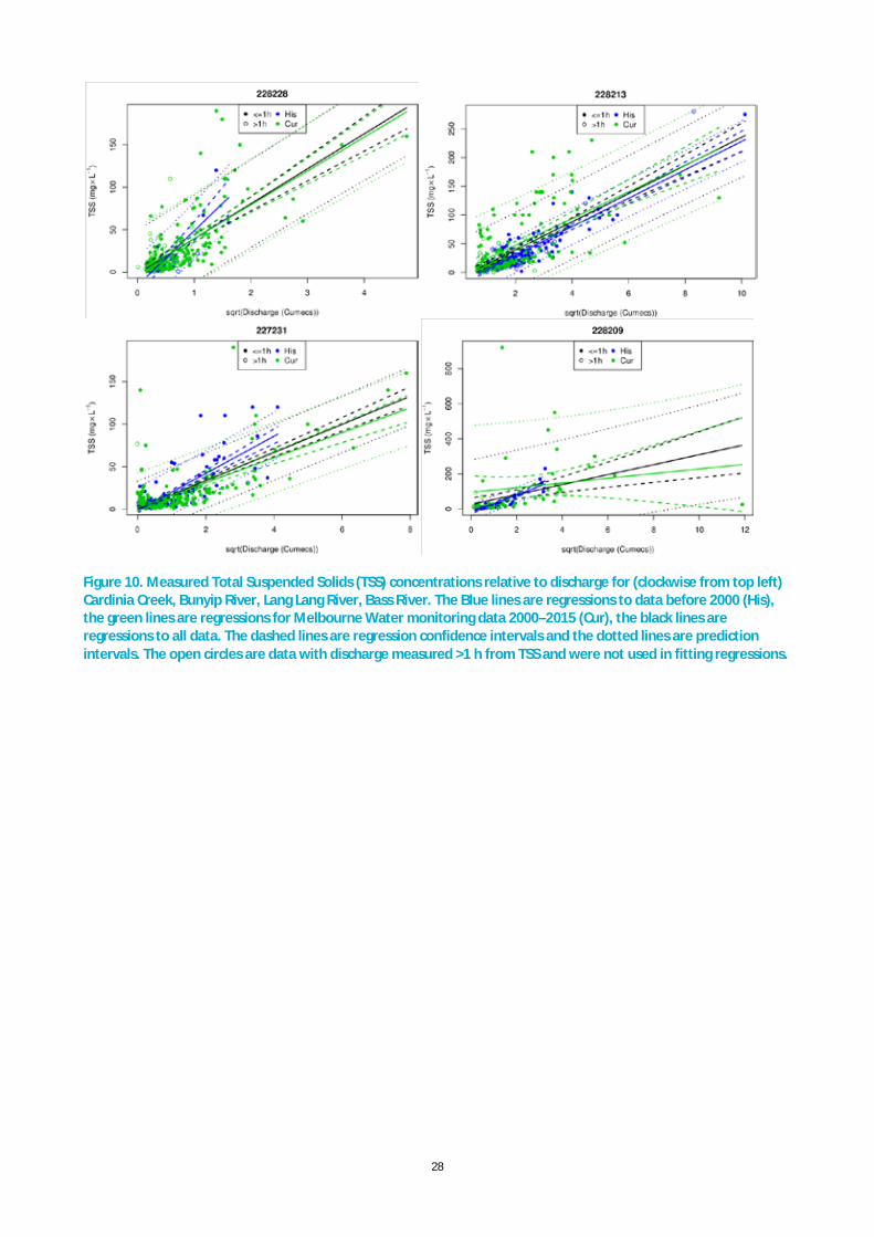
28

Figure 10. Measured Total Suspended Solids (TSS) concentrations relative to discharge for (clockwise from top left) Cardinia Creek, Bunyip River, Lang Lang River, Bass River. The Blue lines are regressions to data before 2000 (His), the green lines are regressions for Melbourne Water monitoring data 2000–2015 (Cur), the black lines are regressions to all data. The dashed lines are regression confidence intervals and the dotted lines are prediction intervals. The open circles are data with discharge measured >1 h from TSS and were not used in fitting regressions.

29

Figure 11. Measured Total Nitrogen (TN) concentrations relative to discharge for (clockwise from top left) Cardinia Creek, Bunyip River, Lang Lang River, Bass River. The Blue lines are regressions to data before 2000 (His), the green lines are regressions for Melbourne Water monitoring data 2000–2015 (Cur), the black lines are regressions to all data. The dashed lines are regression confidence intervals and the dotted lines are prediction intervals. The open circles are data with discharge measured >1 h from TN and were not used in fitting regressions.

30

Figure 12. Measured Total Phosphorus (TP) concentrations relative to discharge for (clockwise from top left) Cardinia Creek, Bunyip River, Lang Lang River, Bass River. The Blue lines are regressions to data before 2000 (His), the green lines are regressions for Melbourne Water monitoring data 2000–2015 (Cur), the black lines are regressions to all data. The dashed lines are regression confidence intervals and the dotted lines are prediction intervals. The open circles are data with discharge measured >1 h from TP and were not used in fitting regressions.

2.6.2 SYNTHESIS OF PRIOR SEDIMENT LOAD ESTIMATES

Bay sediment aggradation rates

The silt and clay load indicated by sediment aggradation rates from dating bay sediment cores is based on an estimate that the east bay Corinella and Rhyll segments have experienced sediment aggradation over 1895–2000 of 70–100 kt/y (Hancock et al., 2001); the mid-point of this range is shown in Figure 8. Tides and wind-driven waves redistribute sediment from the Upper North Arm, into which Cardinia Ck, Bunyip and Lang Lang Rivers deliver, into the Corinella and Rhyll sediments (Hancock et al., 2001). Consequently, the Upper North Arm has much lower aggradation rates than Corinella and Rhyll segments. Sediment cores from the Upper North Arm show approximately 30% decline in silt and clay content since 1958 which is shown in Figure 8 (Hancock et al., 2001). This decline suggests either a reduction in catchment fine sediment supply from catchments, or possibly but less likely, an increase in sediment transport capacity in this area associated with reduction in seagrass coverage.

SedNet modelling

The SedNet model constructs mean-annual budgets of fine (silt and clay) and coarse (sand and gravel) sediment sources, transport and deposition for each link in a river network (Wilkinson et al., 2004). It was used to estimate mean-annual sediment loads (Hughes et al., 2003; Wallbrink et al., 2003a). The modelling estimated total silt and clay load of 62 kt y-1, finding that the Bunyip and Lang Lang Rivers together delivered the majority of river sediment to the bay. The modelling period included Cardinia and Tarago Reservoirs constructed after 1940. These are likely to have had a minor effect on total catchment loads but may have elevated river TSS concentrations during the construction period.

31

Sediment source tracing

Sediment source tracing has been used to identify the sources of clay sediment (<4 µm) in Western Port (Wallbrink et al., 2003a; Wallbrink et al., 2003b). The sediment tracing study did not estimate river loads directly, but did estimate the relative contributions of each river to the bay sediments. For the Bunyip and Lang Lang River contributions, these two sets of estimates were regarded as in agreement considering uncertainties (Wallbrink et al., 2003a). Tracing predicted a relatively larger contribution of Cardinia Creek than SedNet modelling, which was attributed to construction of the Cardinia Reservoir, which may have released a pulse of material and has since trapped all sediment from the upper part of that catchment. Yallock Creek contributions may have been underestimated by the source tracing but can be considered to be relatively small.

This study also concluded that 68% of clay in the north arm sediments, and 70% in the south bay (Corinella and Rhyll segments), was derived from river sediment, with the remainder from erosion of coastal clay banks near Lang Lang, which we use below to estimate total loads from coastal bank erosion rates.

Coastal bank erosion

A study of the extent of those coastal banks and their erosion rates using air photos estimated that they have eroded at 0.3 m/y on average over the period 1947–2013, supplying 4.2 ± 2.9 kt yr-1 (Tomkins et al., 2014). The sediment yield varied in the range 2.8–9.4 kt/y over different periods within time. The silt and clay content of bank soil was measured at 17% and 60%, respectively. A similar study based on a slightly longer length of coastline estimated a higher mean erosion rate of 0.5 m/y for the period 1977–2012 (Hurst, 2012). When converted to yield based on the bank heights and soil properties observed by (Tomkins et al., 2014) this study estimated a yield of 5.2 kt/y.

These estimates of coastal bank sediment supply were combined with the above source tracing estimate of 32% contribution to the <10 µm fraction of bay sediments from coastal banks (based on sediment samples collected in 2000), and the particle size distribution of river sediment and coastal bank soil, to estimate total coastal bank and river silt and clay inputs of 25 and 31 kt y-1, respectively. Source tracing applies to only the clay component of the river and coastal bank sediment loads. The total load estimate was based on taking the coastal bank clay contribution at 32% of the clay load from all sources. Coastal bank soil is 60% clay, giving a coastal bank clay load of 2.5 ± 1.7 kt yr-1, while we assumed that clay comprises 14% of river load (equal to that of river bed sediment deposits).

The upper layers of bay sediments were well-mixed (Hancock et al., 2001), indicating that the sediment source tracing based on geochemistry, and hence the total load estimate based on coastal bank erosion, applies to at least several decades.

Previous TSS monitoring at river gauges

Based on TSS monitoring during 1973–1976, and linear sediment-discharge rating curves, a mean-annual load of 65 kt yr-1 was estimated for all rivers draining into Western Port, of which 30 kt yr-1 was derived from the Lang Lang and Bunyip Rivers alone (Sargeant, 1977; Dale and Pooley, 1979). Over a longer period 1980–1998 a somewhat lower estimate of 31 kt yr-1 delivered to Western Port can be derived from the work of Lowe (1999).

The load estimate of Sargeant et al., (1977) and Dale and Pooley (1979) is higher than other load estimates based on TSS monitoring. The main reason is that reported mean discharge in that period was four times the average over 1980—2014. Mean concentrations at that time were not apparently higher. Linear regressions between measured load and flow were applied to estimate load from the flow record which may have influenced the estimates.

An independent set of load estimates by Ladson (2016) based on event mean and dry-weather concentrations for the duration of the Melbourne Water Loads program found larger loads than estimated here, with a mean-annual TSS load summed across the four gauges of 20.5 kt/y, 60% larger than our estimate of 12.9 kt/y. Similarly, their total nitrogen and phosphorus loads were also considerably larger.

32

The uncertainty bounds for the two sets of estimates overlap, assuming a ~30% uncertainty in the estimates of Ladson (2016). However, the discrepancy between the best estimates can be attributed to differences in methods. We observed progressive variation in concentration with turbidity, and found that linear regressions against turbidity better represented variations in concentration than did variations with discharge. We multiplied instantaneous discharge by an estimate of instantaneous concentrations. By contrast, Ladson (2016) multiplied daily averages of discharge by the mean concentration for event or dry weather conditions, rather than representing progressive increases in concentration with discharge (e.g., Figure 10). The method of Ladson (2016) was also sensitive to the criteria used to partition the monitoring period between event and dry weather conditions.

PPBWP Catchment Modelling

A model of catchment runoff was used to estimate TSS, TN and TP loads to Western Port for the period 1995–2011 using the “Port Phillip Bay and Western Port Catchment Model” (Stewart, 2012). This model calculated load as the product of daily runoff volume and constituent concentrations for dry weather and event mean concentration. Runoff was modelled using the SIMHYD conceptual model calibrated to stream gauge data. Constituent concentrations were derived from earlier studies in the area. The model covered the entire 3,300 km2 area draining to Western Port (Figure 3). The four catchments studied here plus Yallock Creek (between Bunyip River and Lang Lang River) comprise 70% of this total area. The PPBWP catchment model estimated a TSS delivery to the bay of 11.8 kt y-1 (Catchment Research pty ltd, 2012). This estimate included 8.8 kt y-1 from the five catchments including Yallock Creek.

33

3 Channel sediment delivery

3.1 Objectives

This activity involved applying a hydrodynamic and sediment transport model to the four river channels for which loads were estimated at the river gauges (Cardinia Creek, Bunyip River, Lang Lang River and Bass River). The main objectives of this research activity were:

1. To inform the translation of river loads estimated in Section 2 from the gauging stations to the river mouths where the hydrodynamic model of Western Port requires load inputs.

2. To map erosion and deposition zones in the above major streams. Previous SedNet modelling identified some reaches of these streams within the floodplain as having high rates of bank erosion (Hughes et al., 2003). However, channel slopes are relatively low and the channels have been artificially enlarged to accommodate flood flows, which can be expected to reduce velocities.

The research investigated sediment transport dynamics in these channels above the tidal limits, including consideration of the various size fractions, scale effects on transit times and lags (i.e. the impact of distance downstream from source) and the flow conditions during which sediments are transported to end of system and input into the bay. It was postulated that a persistent relationship between stream discharge and net sediment transport may exist in channelized reaches, with deposition occurring at lower discharges and higher connectivity and channel erosion at higher discharges.

3.2 Methods

Sediment transport modelling

Sediment transport modelling was carried out using the HEC-RAS (Hydraulic Engineering Center - River Analysis System package version 4.1; http://www.hec.usace.army.mil/software/hec-ras/) hydraulic model to simulate channel erosion, deposition and transient storage during flow events. The main inputs to the model include stream cross-section, particle size of bed material, surface roughness in terms of Manning roughness coefficient and flow and stage height data for model boundaries. The model outputs include changes in bed profile over the simulation period and time-series of erosion and deposition. A separate hydrodynamic and sediment transport model was configured for each channel (Cardinia Creek and Bunyip, Lang Lang and Bass rivers; Figure 13).

34

Figure 13 Port Bay catchment showing major rivers and creeks. The red triangle shows the name and location of gauging stations and the orange circle represents the location of stream photos shown in the next figure

Sediment computations in HEC-RAS utilize one dimensional, cross-section averaged, hydraulic properties to compute sediment transport rates and update the channel geometry based on sediment continuity calculations. HEC-RAS utilizes quasi-steady hydrodynamics, which involves applying constant flow within each day, but running at time-steps of minutes to hours to represent changes in channel cross sections resulting from erosion or deposition. A transport equation was selected. Total transport capacity was calculated independently for each size class and then weighted by the relative abundance in the active bed layer. Net erosion/deposition at any location depended on incoming sediment at that location and sediment carrying capacity at a particular time.

Model inputs

Stream cross-sections were extracted from a LiDAR DEM at 1 m resolution, at 1 km interval along the channel centreline. LiDAR data were supplied by Melbourne Water as a mixture of ascii 1m gridded xyz points and irregularly spaced points. These data were processed and a 1 m resolution DEM was produced.

Channel cross section shape, longitudinal slope, vegetation cover and sediment particle size distributions were measured in the field or in prior surveys at several locations across the Cardinia, Bunyip, Lang Lang and Bass rivers. The 2010 Index of Stream Condition assessment data (Wilson, 2014) was used to inform patterns of channel width and depth, and indicators of bank erosion.

Particle size data for bed materials were calculated from sampled bed material deposits. Sediment samples were collected at 21 sites in 2 creeks and 3 rivers in September 2014 and analysed at CSIRO Black Mountain laboratories.

The hydrodynamic component of the HEC-RAS model was calibrated using observed stage height and discharge. The sediment transport component of the model was calibrated by comparison with observed

35

annual TSS loads at the river gauges (from Section 2.3.2). This involved selecting the most suitable sediment transport equation. Ideally the sediment transport calibration uses the observed bed elevation data at different time periods and/or total sediment loads, however this was not possible within the time available.

One limitation of the modelling is that it did not represent the effect of benthic vegetation to reduce the shear stress applied to channel banks and bed in floodplain reaches, although large parts of the channel banks and bed in these reaches are colonised by benthic vegetation including Phragmites spp. It is likely that benthic vegetation enhances deposition at lower flows above what is modelled. The vegetation effect at higher discharge is less clear, although it is likely that vegetation continues to provide some bed protection. Consequently, the relative differences in equilibrium sediment transport rate from the gauge across the floodplain reach were used to indicate net erosion and deposition, rather than absolute rates.

3.3 Results

Channel geometry and vegetation

The channel width was typically 30–50 m bank to bank, with inset channels of about 10–20 m width. In general the channel cross sections consist of wide river berms above the main channel and then a steep bank down to the river bed (Figure 14). The vegetation is dense and high in many areas. However, during high flows bank erosion can occur along the river channel.

The ISC 2010 data indicates that river bank heights are highest in the Bass River and along some middle and upper reaches of the Cardinia, Bunyip and Lang Lang Rivers (Figure 15). The width of vegetation beside streams is generally lower in floodplain reaches than further upstream, particularly in the Cardinia, Bunyip and Lang Lang Rivers. These data are confined to the trunk streams, which is suitable for this research. However, because of that, they do not provide overall priorities for catchment management.

36

(a)

(b)

(c)

(d)

Figure 14 River cross sections for a) Cardinia Creek, b) Bunyip River, c) Lang Lang River and d) Bass River, within the floodplain reaches of these streams (locations are shown in Figure 13)

Figure 15 Left: River bank height (left) and width of vegetation (right) for each 100 m section of stream, as assessed for the Index of Stream Condition 2010 (Wilson, 2014).

The hydrodynamic model for Cardinia Creek consists of 30 cross-sections defining its upstream boundary at the Beaconsfield Upper and downstream boundary just above the Gippsland Highway (Figure 16). There is a sharp fall in river bed elevation above just below Cardinia, increasing sediment carrying capacity. In most

37

places Cardinia Creek is a single channel stream, with more than one channel at some locations especially downstream of Cardinia (Figure 17).

Figure 16 River bed profile of Cardinia Creek based on LiDAR 1m DEM

a)

b)

Figure 17 Typical example of stream cross-sections: a) single channel 3 km upstream of Cardina, b) multiple channels at Ballarto Road Crossing, 5 km upstream of Gippsland Highway. The values above each plot illustrate how different channel roughness values were applied to the channel and floodplain segments of cross sections.

-20

0

20

40

60

80

100

120

0.0 5.0 10.0 15.0 20.0 25.0 30.0 35.0

Elev

atio

n (m

, AHD

)

Distance from river mouth (km)

Gippsland Highway

Cardinia

Beaconsfield

Beaconsfield Upper

0 200 400 600 8018

20

22

24

26

28

Station (m)

Ele

vatio

n (m

)

.06 .035 .06

0 200 400 600 800

1

2

3

4

5

6

7

Station (m)

Ele

vatio

n (m

)

.06 .035 .06

38

Sediment characteristics

The sediment dry bulk density was typically 1.2–1.3 g cm-3 (Table 3). Particle size distributions of bed material indicate that Bunyip River sediment contains less fine material than other streams (Figure 18). The relative differences in average clay content of sediment between rivers were consistent with an earlier study, although absolute values differed (Table 4).

Table 3 Bulk density of bed material across each river

RIVER LOCATION BULK DENSITY, OVEN DRY (G/CM3)

BULK DENSITY, FRESH WEIGHT (G/CM3)

Cardinia Dalmore Road 1.34 1.66

Cardinia Chasemore Road 1.17 1.65

Cardinia Princes Highway 1.17 1.57

Cardinia Inglis Road 1.24 1.48

Bunyip Princes Highway 1.20 1.48

Bunyip Evans Road 1.24 1.67

Bunyip Main Drain Road 1.22 1.53

Bunyip Pitt Road 1.21 1.51

Yallock Coster Road 1.30 1.68

Yallock Modella (on Koo wee Rup Road) 1.17 1.69

Yallock Fincks Road 0.90 1.28

Yallock No. 5 Drain Road 0.71 1.27

Lang Lang Drouin Poowong Road 1.24 1.66

Lang Lang Western Port Road 1.25 1.76

Lang Lang Patullos Road 1.49 1.85

Lang Lang Heads Road 1.48 1.88

Bass Ferriers Road 1.23 1.53

Bass Woodleigh Road 1.09 1.60

Bass Stewart Road 0.97 1.54

Bass Grantville Road 1.06 1.63

Bass Glen Forbes 1.28 1.62

Table 4 Clay component (particle size < 4µm) of bed material in each river

RIVER OR CREEK MEAN (%) MINIMUM (%) MAXIMUM (%)

Present study Wallbrink et al. (2003)

Present study Wallbrink et al. (2003)

Present study Wallbrink et al. (2003)

Cardinia Creek 18.85 27.52 8.05 4.22 25.11 64.83

Bunyip River 13.82 5.70 10.82 1.09 16.60 12.97

Lang Lang River 18.11 19.05 13.78 1.78 25.70 53.97

Bass River 16.79 8.52 12.96 1.15 23.07 24.11

39

Figure 18 Cumulative bed material particle size distributions for Western Port rivers

Sediment transport

The model was run for the period of 1/01/2013 to 31/12/2013 at a 0.1 daily time step. Inflow sediment loads were estimated assuming an equilibrium condition (i.e. no erosion or deposition). Time series of daily sediment concentration at river stations were estimated from model results and compared with water quality monitoring data (Figure 19). It is noted that sediment delivery also depends on sediment availability at a particular location and time.

Figure 19 Observed and modelled sediment concentrations relative to stream discharge at Cardinia, based on a daily time series for 2013, and compared with the observed sediment concentrations estimated in Section 2.

In Cardinia Creek, total sediment load increased downstream. Between Cardinia and Dalmore (just before the creek joins with Dalmore main drain), the annual total sediment (suspended and bed load) increased by 4%. Results show that upper reaches of Cardinia Creek experienced up to 60 cm net erosion during the modelled period, while the lower floodplain part experienced 40 cm net deposition. River bed slope was the primary difference between these two reaches.

Sensitivity of model results

The model was applied for 2011 and 2013 calendar years to verify model predictions in different flow events. Predicted sediment loads were compared with estimated sediment loads from river monitoring

0

20

40

60

80

100

0.001 0.01 0.1 1 10

% F

iner

Paticle size (mm)

Cardinia CreekBunyip RiverLang Lang RiverBass River

0

20

40

60

80

100

120

-1.20 -0.70 -0.20 0.30 0.80

Sedi

men

t con

cent

ratio

n (m

g/L)

log10 (Discharge, m3/s)Observed Modelled

40

data and a best performing transport function was selected. Out of seven transport functions three methods (England-Hansen, Toffaleti, Wilcock) produced yearly sediment loads similar to river monitoring data but none of the method produces best results for all four river channels. The England-Hansen (1967) method produced better sediment estimates for the Bunyip and Lang Lang rivers and the Toffaleti (1968) method produced better estimates for Cardinia Creek and Bass River. Results were relatively insensitive to particle fall velocity method.

Surface roughness was an important factor in transport estimation. An analysis based on sub-daily sediment transport rate of Cardinia Creek indicated the predicted annual sediment load could be up to 18% more for a relatively less vegetated river (Manning’s n of 0.03 for river and 0.04 for floodplain) and 30% less for a dense vegetated river (Manning’s n of 0.05 for river and 0.1 for floodplain) compared to standard settings (Manning’s n of 0.035 for river and 0.06 for floodplain).

Sediment delivery to the bay

A sediment delivery ratio (SDR), being the sediment transport rate at the catchment outlet divided by that at the stream gauging site, was estimated as a function of stream discharge. Often this relationship was variable at small flow because of large variations in predicted delivery rates. Also, for small flow, modelled load was relatively small compared to observed data (Figure 19). In this analysis, a 30 points moving average method was applied to smooth out the SRD. The SRD could be less or more than one based on floodplain configuration and gauge location.

Figure 20 Sediment delivery ratio between catchment outlet (4.8 km from river mouth) and Glen Forbes gauge (13 km from the river mouth) for the Bass River. Results presented are based on daily time series of sediment delivery rate in 2011 and 2013.

Efforts were made to derive a relationship between the SDR and stream discharge (here it is the ratio of discharge to median discharge). Simulated daily time series data for the period of 2011 and 2013 were used to construct the SDR ratios for four major river systems in the Western port bay. Results show that sediment to the bay could be less or more than that are recorded at the gauge.

Based on the two years studied, the typical SDR variations with discharge were as follows:

Cardinia Creek:

𝑆𝑆𝑆𝑆𝑆𝑆 = 1 − 0.05𝑄𝑄 𝑖𝑖𝑖𝑖 𝑄𝑄 ≤ 2.0 = 0.9 𝑖𝑖𝑖𝑖 𝑄𝑄 > 2.0 �

0.90

0.95

1.00

1.05

1.10

1.15

1.20

1.25

1.30

0.0 10.0 20.0 30.0 40.0 50.0 60.0

Sedi

men

t del

iver

y ra

tio

Discharge (m3/s)

All time-stepsMoving average

41

Bunyip River:

𝑆𝑆𝑆𝑆𝑆𝑆 = 1.3 𝑖𝑖𝑖𝑖 𝑄𝑄 ≤ 2.0 = 1.5 − 0.1𝑄𝑄 𝑖𝑖𝑖𝑖 𝑄𝑄 > 2.0 𝑎𝑎𝑎𝑎𝑎𝑎 ≤ 5.0

= 1.0 𝑖𝑖𝑖𝑖 𝑄𝑄 > 5.0�

Lang Lang River:

𝑆𝑆𝑆𝑆𝑆𝑆 = 1.2 𝑖𝑖𝑖𝑖 𝑄𝑄 ≤ 1.0 = 1.24 − 0.04𝑄𝑄 𝑖𝑖𝑖𝑖 𝑄𝑄 > 1.0 𝑎𝑎𝑎𝑎𝑎𝑎 ≤ 5.0

= 1.04 𝑖𝑖𝑖𝑖 𝑄𝑄 > 5.0�

Bass River:

𝑆𝑆𝑆𝑆𝑆𝑆 = 1.10 𝑖𝑖𝑖𝑖 𝑄𝑄 ≤ 1.0 = 1.16 − 0.02𝑄𝑄 𝑖𝑖𝑖𝑖 𝑄𝑄 > 1.0 𝑎𝑎𝑎𝑎𝑎𝑎 ≤ 8.0

= 1.0 𝑖𝑖𝑖𝑖 𝑄𝑄 > 8.0�

Figure 21 Sediment delivery ratio to estimate catchment sediment delivery from the stream gauges to Western Port for the Cardinia, Bunyip, Lang Lang and Bass rivers

While erosion and deposition can happen at any discharge based on sediment input and carrying capacity, with some exceptions, deposition occurs at low flow and erosion occurs at high flow (Figure 22). This is broadly consistent with the relationship we postulated, with the refinements that net deposition is zero at zero discharge and the rates of deposition are relatively smaller compared to erosion. The much shorter duration of discharge above the daily median value means that the accrued net erosion is close to zero. As previously noted, this method tends to over-estimate the absolute magnitude of delivery ratio because it does not account for bed armouring by vegetation, or for short deposition locations within the floodplain channels. It may underestimate the delivery ratio where large tributaries join downstream of the gauge, increasing sediment transport capacity of the flow.

0.80

0.90

1.00

1.10

1.20

1.30

1.40

0 5 10 15 20 25 30

Sedi

men

t del

iver

y ra

tio

Q/Qmedian

Cardinia BunyipLang Lang Bass

42

Figure 22 Erosion and deposition rate as a function of stream discharge for Cardinia Creek

Spatial distribution of erosion and deposition along a river profile have been estimated from time series of sediment loads. Net erosion at a particular location is estimated by subtracting incoming sediment from outgoing sediment as a sequence of time. Therefore, a positive value indicates erosion at that point and a negative value indicates deposition. This information is useful to identify potential sources of sediment and places of sediment deposition. For Cardinia Creek (Figure 23), net deposition is most likely in reaches above Beaconsfield, downstream of Beaconsfield and downstream of Cardinia. The deposition status in other rivers was more spatially uniform (Figure 24; Figure 25; Figure 26).

Figure 23 Spatial distribution of erosion and deposition along Cardinia Creek. A positive value indicates a sediment source and a negative value indicates sediment sink. Results are based on a simulation period of 1/01/2013 to 31/12/2013.

-2.0

-1.0

0.0

1.0

2.0

3.0

4.0

0.00 1.00 2.00 3.00 4.00 5.00 6.00 7.00 8.00

Eros

ion

(t/d

ay)

Q/Qmedian

Depo

sitio

n

-3.0

-2.0

-1.0

0.0

1.0

2.0

0 5 10 15 20 25 30 35

Net

ero

sion

(kt/

yr)

Distance from river mouth (km)

Gippsland Highway Cardinia Beaconsfield Beaconsfield

Upper

43

Figure 24 Spatial distribution of erosion and deposition along the Bunyip River. A positive value indicates a sediment source and a negative value indicates sediment sink. Results are based on a simulation period of 1/01/2013 to 31/12/2013.

Figure 25 Spatial distribution of erosion and deposition along the Lang Lang River. A positive value indicates a sediment source and a negative value indicates sediment sink. Results are based on a simulation period of 1/01/2013 to 31/12/2013.

Figure 26 Spatial distribution of erosion and deposition along the Bass River. A positive value indicates a sediment source and a negative value indicates sediment sink. Results are based on a simulation period of 1/01/2013 to 31/12/2013.

-0.5

-0.3

0.0

0.3

0.5

0.8

1.0

0 10 20 30 40 50 60

Net

ero

sion

(kt/

yr))

Distance from river mouth (km)

Gippsland Highway

Iona Bunyip Tonimbuk Headworks

-1.0

0.0

1.0

2.0

3.0

4.0

0 5 10 15 20 25 30 35 40

Net

ero

sion

(kt/

yr)

Distance from river mouth (km)

Gippsland Highway

Lang Lang Heath Hill

-0.5

-0.3

0.0

0.3

0.5

0.8

1.0

0 5 10 15 20 25 30 35

Net

ero

sion

(kt/

yr))

Distance from river mouth (km)

Gippsland HighwayGlen Forbes Lock

44

3.4 Model limitations

Results obtained using the HEC-RAS hydrodynamic model possess large uncertainties in load estimates because of its sensitivity to sediment transport functions, and to a lesser degree channel roughness. Major limitations of the model are that it considers a quasi-unsteady flow condition. Results may be improved to some extent by using a fully unsteady hydrodynamic model, such as MIKE 11. However, both HEC-RAS and MIKE 11 models are one dimensional and are not capable of estimating cross-sectional changes of rivers. It is recommended that a two dimensional model (e.g. MIKE 21) would be required to represent detail information on spatial and temporal changes in erosion and deposition.

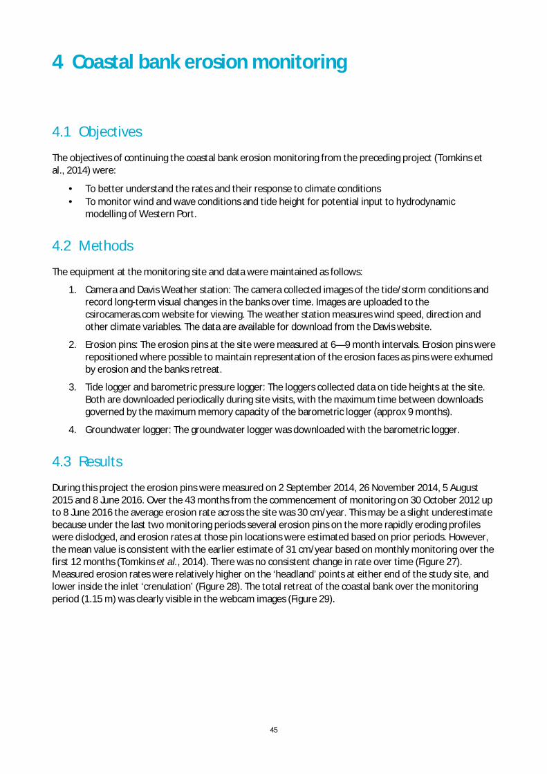
45

4 Coastal bank erosion monitoring

4.1 Objectives

The objectives of continuing the coastal bank erosion monitoring from the preceding project (Tomkins et al., 2014) were:

· To better understand the rates and their response to climate conditions · To monitor wind and wave conditions and tide height for potential input to hydrodynamic

modelling of Western Port.

4.2 Methods

The equipment at the monitoring site and data were maintained as follows:

1. Camera and Davis Weather station: The camera collected images of the tide/storm conditions and record long-term visual changes in the banks over time. Images are uploaded to the csirocameras.com website for viewing. The weather station measures wind speed, direction and other climate variables. The data are available for download from the Davis website.

2. Erosion pins: The erosion pins at the site were measured at 6—9 month intervals. Erosion pins were repositioned where possible to maintain representation of the erosion faces as pins were exhumed by erosion and the banks retreat.

3. Tide logger and barometric pressure logger: The loggers collected data on tide heights at the site. Both are downloaded periodically during site visits, with the maximum time between downloads governed by the maximum memory capacity of the barometric logger (approx 9 months).

4. Groundwater logger: The groundwater logger was downloaded with the barometric logger.

4.3 Results

During this project the erosion pins were measured on 2 September 2014, 26 November 2014, 5 August 2015 and 8 June 2016. Over the 43 months from the commencement of monitoring on 30 October 2012 up to 8 June 2016 the average erosion rate across the site was 30 cm/year. This may be a slight underestimate because under the last two monitoring periods several erosion pins on the more rapidly eroding profiles were dislodged, and erosion rates at those pin locations were estimated based on prior periods. However, the mean value is consistent with the earlier estimate of 31 cm/year based on monthly monitoring over the first 12 months (Tomkins et al., 2014). There was no consistent change in rate over time (Figure 27). Measured erosion rates were relatively higher on the ‘headland’ points at either end of the study site, and lower inside the inlet ‘crenulation’ (Figure 28). The total retreat of the coastal bank over the monitoring period (1.15 m) was clearly visible in the webcam images (Figure 29).

46

Figure 27 Average coastal bank erosion rates over the period prior to each monitoring date. A linear regression is fitted to the data.

Figure 28 (Left) Average coastal bank erosion rates at each monitoring profile over 33 months to August 2015. (Right) Location of each erosion pin profile (Tag) at the site, reproduced from (Tomkins et al., 2014).

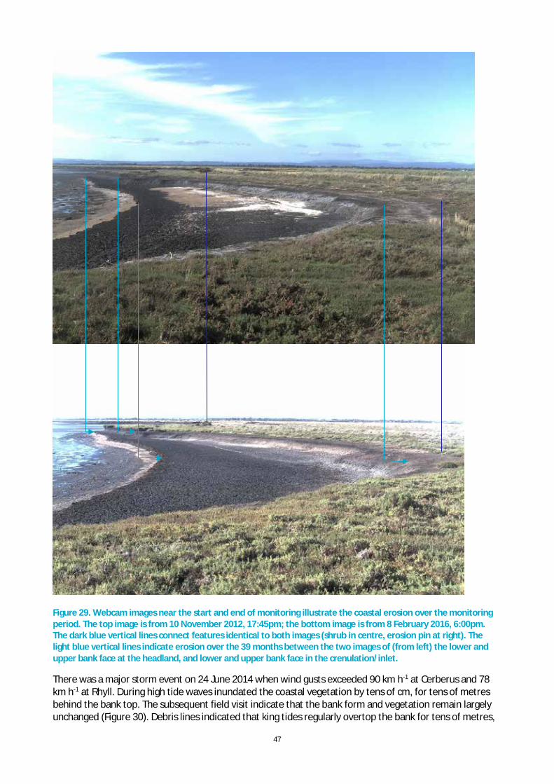
47

Figure 29. Webcam images near the start and end of monitoring illustrate the coastal erosion over the monitoring period. The top image is from 10 November 2012, 17:45pm; the bottom image is from 8 February 2016, 6:00pm. The dark blue vertical lines connect features identical to both images (shrub in centre, erosion pin at right). The light blue vertical lines indicate erosion over the 39 months between the two images of (from left) the lower and upper bank face at the headland, and lower and upper bank face in the crenulation/inlet.

There was a major storm event on 24 June 2014 when wind gusts exceeded 90 km h-1 at Cerberus and 78 km h-1 at Rhyll. During high tide waves inundated the coastal vegetation by tens of cm, for tens of metres behind the bank top. The subsequent field visit indicate that the bank form and vegetation remain largely unchanged (Figure 30). Debris lines indicated that king tides regularly overtop the bank for tens of metres,

48

and up to 50 cm of organic debris blanketed the ground in places along the earthen sea wall. It appeared that the vegetation behind the coastal bank became sparser during the monitoring period. The bank face continued to show evidence of mass wasting, accentuated by the twice daily wetting and drying. Much of the eroding surface had a ‘honeycomb’ appearance perhaps associated with variations in organic matter. In the headland sections the bank face was steeper, and the more rapid erosion rate there occurred through scour of the bank toe accompanied by mass failure of the middle and upper parts of the bank profile, as indicated by tension cracks and debris blocks of bank material (Figure 31). There was little debris present relative to the rate of erosion, indicating that wave action during high tide periods was efficient at breaking down the debris and transporting eroded material away.

Figure 30 Left: Coastal bank erosion monitoring site at 11:45 am on 24 June 2014. Right: the site on 26 November 2014.

Figure 31 Left: Vegetation density affected by wave inundation behind the crenulation section. Right: Looking downwards showing tension cracks running along the top of the lower bank adjacent to the headland at the southern end of the site.

The erosion pins were monitored finally in June 2016 and the site decommissioned. Six star pickets were installed as reference markers and located with a RTK GPS. A handheld laser scanner was used to generate a high-resolution DEM (digital elevation model) of the ground surface at the site, which could be used as a baseline for repeat scans to estimate erosion over coming years. The weather data are available on the data access portal https://data.csiro.au/dap, by searching for “Western Port”.

49

Figure 32 Coastal bank erosion site during high tide, 9 October 2012.

Sea level is likely to rise 44—74 cm or possibly more by 2100, depending on emissions scenarios (Church et al., 2013). It is expected that this will exacerbate coastal erosion as coastal vegetation becomes degraded, and control measures will need to be adaptable to continued sea level rise.

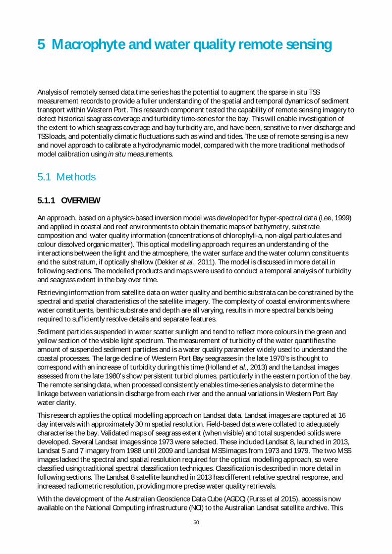
50

5 Macrophyte and water quality remote sensing

Analysis of remotely sensed data time series has the potential to augment the sparse in situ TSS measurement records to provide a fuller understanding of the spatial and temporal dynamics of sediment transport within Western Port. This research component tested the capability of remote sensing imagery to detect historical seagrass coverage and turbidity time-series for the bay. This will enable investigation of the extent to which seagrass coverage and bay turbidity are, and have been, sensitive to river discharge and TSS loads, and potentially climatic fluctuations such as wind and tides. The use of remote sensing is a new and novel approach to calibrate a hydrodynamic model, compared with the more traditional methods of model calibration using in situ measurements.

5.1 Methods

5.1.1 OVERVIEW

An approach, based on a physics-based inversion model was developed for hyper-spectral data (Lee, 1999) and applied in coastal and reef environments to obtain thematic maps of bathymetry, substrate composition and water quality information (concentrations of chlorophyll-a, non-algal particulates and colour dissolved organic matter). This optical modelling approach requires an understanding of the interactions between the light and the atmosphere, the water surface and the water column constituents and the substratum, if optically shallow (Dekker et al., 2011). The model is discussed in more detail in following sections. The modelled products and maps were used to conduct a temporal analysis of turbidity and seagrass extent in the bay over time.

Retrieving information from satellite data on water quality and benthic substrata can be constrained by the spectral and spatial characteristics of the satellite imagery. The complexity of coastal environments where water constituents, benthic substrate and depth are all varying, results in more spectral bands being required to sufficiently resolve details and separate features.

Sediment particles suspended in water scatter sunlight and tend to reflect more colours in the green and yellow section of the visible light spectrum. The measurement of turbidity of the water quantifies the amount of suspended sediment particles and is a water quality parameter widely used to understand the coastal processes. The large decline of Western Port Bay seagrasses in the late 1970’s is thought to correspond with an increase of turbidity during this time (Holland et al., 2013) and the Landsat images assessed from the late 1980’s show persistent turbid plumes, particularly in the eastern portion of the bay. The remote sensing data, when processed consistently enables time-series analysis to determine the linkage between variations in discharge from each river and the annual variations in Western Port Bay water clarity.

This research applies the optical modelling approach on Landsat data. Landsat images are captured at 16 day intervals with approximately 30 m spatial resolution. Field-based data were collated to adequately characterise the bay. Validated maps of seagrass extent (when visible) and total suspended solids were developed. Several Landsat images since 1973 were selected. These included Landsat 8, launched in 2013, Landsat 5 and 7 imagery from 1988 until 2009 and Landsat MSS images from 1973 and 1979. The two MSS images lacked the spectral and spatial resolution required for the optical modelling approach, so were classified using traditional spectral classification techniques. Classification is described in more detail in following sections. The Landsat 8 satellite launched in 2013 has different relative spectral response, and increased radiometric resolution, providing more precise water quality retrievals.

With the development of the Australian Geoscience Data Cube (AGDC) (Purss et al 2015), access is now available on the National Computing infrastructure (NCI) to the Australian Landsat satellite archive. This

51

data has been consistently processed using atmospheric correction technique (Li et al. 2010) and quality assessment flagging methods (Irish 2006), allowing retrieval of surface reflectance from multi-sensor time series for analysis. At the commencement of this project, data availability from the AGDC was limited, therefore data was downloaded from the USGS site. However, data was later acquired in the form of pixel drills, which retrieve data values for a given location for each tile within the time series. These pixel drill are used to construct a multi-sensor time series that can be used to track the relative changes within Western Port with consistent errors across time and across sensors.

In this project, we applied an optical water quality retrieval algorithm to all the Landsat data from USGS and AGDC. The resultant maps and time series plots can be used to conduct a change detection analysis of turbidity and seagrass extent in the bay over time. Images were calibrated using relevant field data (Table 9).

5.1.2 REMOTE SENSING RETRIEVAL MODEL

A physics-based model offers an objective and repeatable algorithm for retrieval of substratum-type information from remote sensing data. An inversion algorithm (Lee et al., 1998; Lee et al., 1999; Lee et al., 2001) was developed for remote sensing data using an analytical model and optimisation routine. The algorithm expresses the subsurface remote-sensing reflectance 𝑟𝑟𝑟𝑟𝑟𝑟 as a function of a set of environmental variables, that is, measureable water properties which can be estimated from remotely sensed data. When the modelled remote sensing reflectance 𝑟𝑟𝑟𝑟𝑟𝑟

𝑚𝑚𝑚𝑚𝑚𝑚𝑚𝑚𝑚𝑚𝑚𝑚𝑚𝑚𝑚𝑚 is compared to the measured satellite remote sensing reflectance 𝑟𝑟𝑟𝑟𝑟𝑟

𝑖𝑖𝑖𝑖𝑖𝑖𝑖𝑖𝑖𝑖, the set of environmental variables that minimises the difference between the model and input reflectance provides the solution. In Wettle and Brando (2006), Brando et al. (2009) and Dekker et al. (2011), the Lee et al. (2001) algorithm was enhanced and evolved into SAMBUCA, a semi-analytical model for bathymetry un-mixing and concentration assessment. SAMBUCA was now able to retrieve simultaneous outputs of:

1. the water’s optically active constituent concentrations (chlorophyll-a, Coloured dissolved organic matter and non-algal particulate),

2. the percentage substratum cover type (either as homogeneous or mixtures of 2 different types) and

3. metrics to assess the reliability of the retrieval.

In summary, the complete model parameterization for SAMBUCA is:

Each parameter is defined in Table 5.

( ) ( )( ) ( )

model * * * *PHY NAP 0 PHY 0 NAP 0

, , , , , , , , ,

, , , , ( ), ( )CHL CDOM NAP i i j CDOM NAP

rsPHY NAP b b

C C C H B S Sr f

Y Y a a b b

r l r l

l l l l

æ ö= ç ÷ç ÷

è ø

52

Table 5: Symbols and definitions of parameters use in the SAMBUCA model

PARAMETER DESCRIPTION UNIT CDOM Coloured dissolved organic matter NAP Non algal particulates λ0 Reference wavelength nm CCHL Concentration of chlorophyll-a µgL-1 CCDOM Concentration of CDOM where 𝑎𝑎𝐶𝐶𝐶𝐶𝐶𝐶𝐶𝐶

∗ (440nm) =1 m-1 CNAP Concentration of NAP mgL-1 H Bottom depth m Bi and Bj Fractional cover of substratum i and substratum j within each pixel % ρi (λ) and ρj (λ) Spectral benthic reflectance (albedo) of substratum i and j - Y Power law exponent for the particulates backscattering coefficient - SCDOM Spectral slope constant of CDOM absorption coefficient nm-1 SNAP Spectral slope constant of NAP absorption coefficient nm-1 𝒂𝒂𝒑𝒑𝒑𝒑𝒑𝒑

∗ (λ) Chlorophyll-a specific absorption spectrum m2mg-1

𝒂𝒂𝑵𝑵𝑵𝑵𝑵𝑵∗ (λ0)

Specific absorption of NAP at reference wavelength m2g-1

𝒃𝒃𝒃𝒃𝒑𝒑𝒑𝒑𝒑𝒑∗ (542nm)

Specific backscattering due to phytoplankton m2mg-1

𝒃𝒃𝒃𝒃𝑵𝑵𝑵𝑵𝑵𝑵∗ (542nm)

Specific backscattering due to NAP m2g-1

𝒓𝒓𝒓𝒓𝒓𝒓𝒎𝒎𝒎𝒎𝒎𝒎𝒎𝒎𝒎𝒎 Modelled subsurface remote-sensing reflectance sr-1

𝒓𝒓𝒓𝒓𝒓𝒓𝒊𝒊𝒊𝒊𝒑𝒑𝒊𝒊𝒊𝒊 sr-1

ENE rsrD Noise equivalent difference in reflectance

IOP Inherent Optical Properties - intrinsic properties not affected by changes in the current radiance distribution

AOP Apparent Optical Properties -those properties dependent on the water’s IOPs and the radiance distribution at the measurement point

Wettle and Brando (2006), Brando et al. (2009) and Dekker et al. (2011) describe a further adaption of SAMBUCA to the reliability of the retrieval in terms of the contribution of the substratum to the remote sensing signal (SDI) and the goodness-of-fit where the modelled remote sensing reflectance is compared to the input provided by the remote sensing data (Δ). The process is illustrated in Figure 33. The Substrate Detectability Index, SDI (Brando et al., 2009; Dekker et al., 2011) was used as an objective method to exclude suboptimal data from the analysis.

Inherent optical properties (IOPs) are the optical properties of water that are independent of the ambient light (Kirk, 1984), such as absorption and scattering. An understanding of the relationship between the reflectance seen by the satellite and the water IOPs is used to invert water quality information from the remotely sensed satellite data. As there is a strong relationship between the IOPs and water quality parameter concentrations, the specific inherent optical property (SIOP) can be derived by normalising the IOPs by its concentration (Campbell et al., 2011).

Inversion methods analysed in (Dekker et al., 2011) showed increased accuracy of retrievals were obtained with improved optical characterisation of the study site. An accurate characterisation or parameterisation provides boundary conditions for the retrieval of the environmental variables. Field campaign measurements ensure the SAMBUCA parameterisation is as robust and comprehensive as possible, but when unavailable, the input is derived from archival field campaign measurements from similar environments. Once parameterised, SAMBUCA was run to estimate the concentrations of optically active constituents in the water column (chlorophyll-a, CDOM and NAP), water column depth, and benthic substratum composition on a pixel-by-pixel basis.

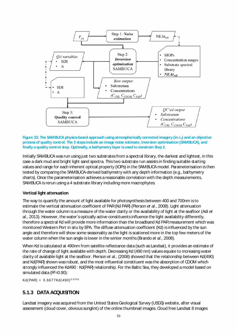
53

Figure 33: The SAMBUCA physics-based approach using atmospherically corrected imagery (in rrs) and an objective process of quality control. The 3 steps include an image noise estimate, inversion optimisation (SAMBUCA), and finally a quality control step. Optimally, a bathymetry layer is used to constrain Step 2.

Initially SAMBUCA was run using just two substrates from a spectral library, the darkest and lightest, in this case a dark mud and bright light sand spectra. This two substrate run assists in finding suitable starting values and range for each inherent optical property (IOPs) in the SAMBUCA model. Parameterisation is then tested by comparing the SAMBUCA-derived bathymetry with any depth information (e.g., bathymetry charts). Once the parameterisation achieves a reasonable correlation with the depth measurements, SAMBUCA is rerun using a 4 substrate library including more macrophytes.

Vertical light attenuation

The way to quantify the amount of light available for photosynthesis between 400 and 700nm is to estimate the vertical attenuation coefficient of PAR (Kd PAR) (Pierson et al., 2008). Light attenuation through the water column is a measure of the water clarity or the availability of light at the seafloor (Adi et al., 2013). However, the water’s optically active constituents influence the light availability differently, therefore a spectral Kd will provide more information than the broadband Kd PAR measurement which was monitored Western Port in situ by EPA. The diffuse attenuation coefficient (Kd) is influenced by the sun angle and therefore will show some seasonality as the light is scattered more in the top few meters of the water column when the sun angle is lower in the winter months (Brando et al., 2008).

When Kd is calculated at 490nm from satellite reflectance data (such as Landsat), it provides an estimate of the rate of change of light available with depth. Decreasing Kd (490 nm) values equate to increasing water clarity of available light at the seafloor. Pierson et al., (2008) showed that the relationship between Kd(490) and Kd(PAR) shown was robust, and the most influential constituent was the absorption of CDOM which strongly influenced the Kd490 : Kd(PAR) relationship. For the Baltic Sea, they developed a model based on simulated data (R2=0.90):

Kd(PAR) = 0.6677Kd(490)0.6763

5.1.3 DATA ACQUISITION

Landsat imagery was acquired from the United States Geological Survey (USGS) website, after visual assessment (cloud cover, obvious sunglint) of the online thumbnail images. Cloud free Landsat 8 images

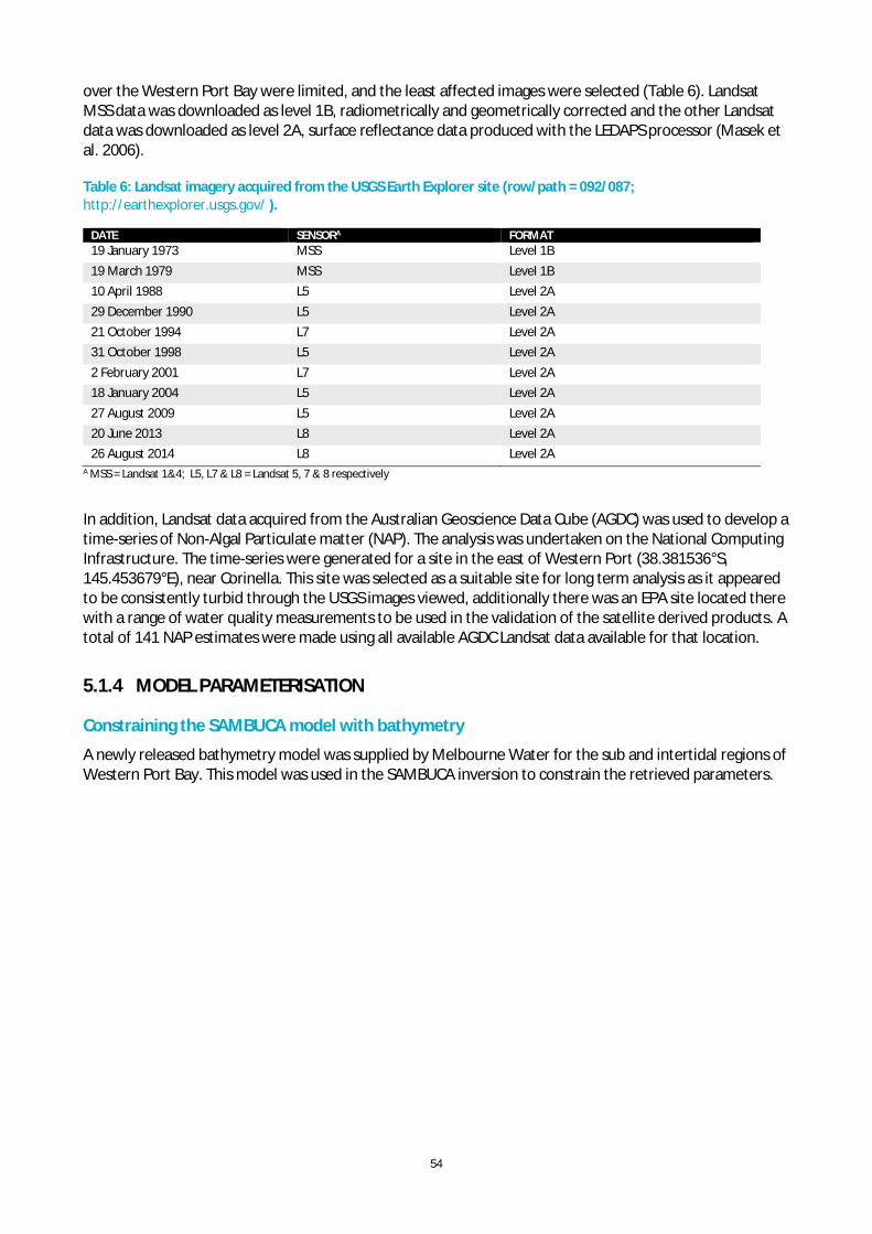
54

over the Western Port Bay were limited, and the least affected images were selected (Table 6). Landsat MSS data was downloaded as level 1B, radiometrically and geometrically corrected and the other Landsat data was downloaded as level 2A, surface reflectance data produced with the LEDAPS processor (Masek et al. 2006).

Table 6: Landsat imagery acquired from the USGS Earth Explorer site (row/path = 092/087; http://earthexplorer.usgs.gov/ ).

DATE SENSORA FORMAT 19 January 1973 MSS Level 1B 19 March 1979 MSS Level 1B 10 April 1988 L5 Level 2A 29 December 1990 L5 Level 2A 21 October 1994 L7 Level 2A 31 October 1998 L5 Level 2A 2 February 2001 L7 Level 2A 18 January 2004 L5 Level 2A 27 August 2009 L5 Level 2A 20 June 2013 L8 Level 2A 26 August 2014 L8 Level 2A

A MSS = Landsat 1&4; L5, L7 & L8 = Landsat 5, 7 & 8 respectively

In addition, Landsat data acquired from the Australian Geoscience Data Cube (AGDC) was used to develop a time-series of Non-Algal Particulate matter (NAP). The analysis was undertaken on the National Computing Infrastructure. The time-series were generated for a site in the east of Western Port (38.381536°S, 145.453679°E), near Corinella. This site was selected as a suitable site for long term analysis as it appeared to be consistently turbid through the USGS images viewed, additionally there was an EPA site located there with a range of water quality measurements to be used in the validation of the satellite derived products. A total of 141 NAP estimates were made using all available AGDC Landsat data available for that location.

5.1.4 MODEL PARAMETERISATION

Constraining the SAMBUCA model with bathymetry

A newly released bathymetry model was supplied by Melbourne Water for the sub and intertidal regions of Western Port Bay. This model was used in the SAMBUCA inversion to constrain the retrieved parameters.

55

Figure 34: Western Port bathymetry from LiDAR and acoustic measurements (source: Melbourne Water).

Parameterisation of the water quality model

The parameterisation requires an understanding of the water columns characteristics, preferably over a range of seasons. In situ measurements and their known ranges were distilled into parameter values for the model. The in situ measurements of inherent optical properties (IOP) such as absorption (a), beam attenuation (c) and scattering (b) were made using in situ profiling instruments (eg WET Labs ac-9 or ac-s). When IOPs are normalized with their biogeochemical concentrations, their mass-specific IOPs (SIOPs) can be estimated (Tilstone et al., 2012).

Figure 35: Averaged specific inherent optical properties (SIOPs) used in the optical model. Data was acquired from field and laboratory measurements.

The Western Port water quality parameterisation was configured from a pre-existing library of IOPs (Figure 35) and published values from literature (Table 7). These data were used to define representative values for Western Port Bay (Table 8).

0

0.5

1

1.5

2

2.5

3

0

0.01

0.02

0.03

0.04

0.05

0.06

0.07

0.08

0.09

400 450 500 550 600 650 700 750 800

a w [m

-1]

a* C

DO

M[-

]

a* PHY

[mg2

mg-1

] a* N

AP[m

g2 m

g-1]

Wavelength (nm)

aw

a*NAP a*

PHY

a*CDOM

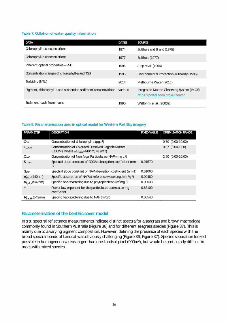
56

Table 7. Collation of water quality information

DATA DATES SOURCE

Chlorophyll-a concentrations 1974 Bulthuis and Brand (1975)

Chlorophyll-a concentrations 1977 Bulthuis (1977)

Inherent optical properties – PPB 1996 Jupp et al. (1996)

Concentration ranges of chlorophyll-a and TSS 1996 Environmental Protection Authority (1996)

Turbidity (NTU) 2014 Melbourne Water (2011)

Pigment, chlorophyll-a and suspended sediment concentrations various Integrated Marine Observing System (IMOS) https://portal.aodn.org.au/search

Sediment loads from rivers 1990 Wallbrink et al. (2003a)

Table 8: Parameterisation used in optical model for Western Port Bay imagery

PARAMETER

DESCRIPTION FIXED VALUE OPTIMIZATION RANGE

CCHL Concentration of chlorophyll-a (µgL-1) 0.70 (0.00-10.00) CCDOM Concentration of Coloured Dissolved Organic Matter

(CDOM) where 𝑎𝑎𝐶𝐶𝐶𝐶𝐶𝐶𝐶𝐶∗ (440nm) =1 (m-1)

0.07 (0.00-1.00)

CNAP Concentration of Non Algal Particulates (NAP) (mg L-1) 2.80 (0.00-10.00) SCDOM Spectral slope constant of CDOM absorption coefficient (nm-

1) 0.01570

SNAP Spectral slope constant of NAP absorption coefficient (nm-1) 0.01060 𝒂𝒂𝑵𝑵𝑵𝑵𝑵𝑵

∗ (440nm) Specific absorption of NAP at reference wavelength (m2g-1) 0.00480 𝒃𝒃𝒃𝒃𝒑𝒑𝒑𝒑𝒑𝒑

∗ (542nm) Specific backscattering due to phytoplankton (m2mg-1) 0.00033

Y Power law exponent for the particulates backscattering coefficient

0.68100

𝒃𝒃𝒃𝒃𝑵𝑵𝑵𝑵𝑵𝑵∗ (542nm) Specific backscattering due to NAP (m2g-1) 0.00540

Parameterisation of the benthic cover model

In situ spectral reflectance measurements indicate distinct spectra for a seagrass and brown macroalgae commonly found in Southern Australia (Figure 36) and for different seagrass species (Figure 37). This is mainly due to a varying pigment composition. However, defining the presence of each species with the broad spectral bands of Landsat was obviously challenging (Figure 36; Figure 37). Species separation looked possible in homogeneous areas larger than one Landsat pixel (900m2), but would be particularly difficult in areas with mixed species.

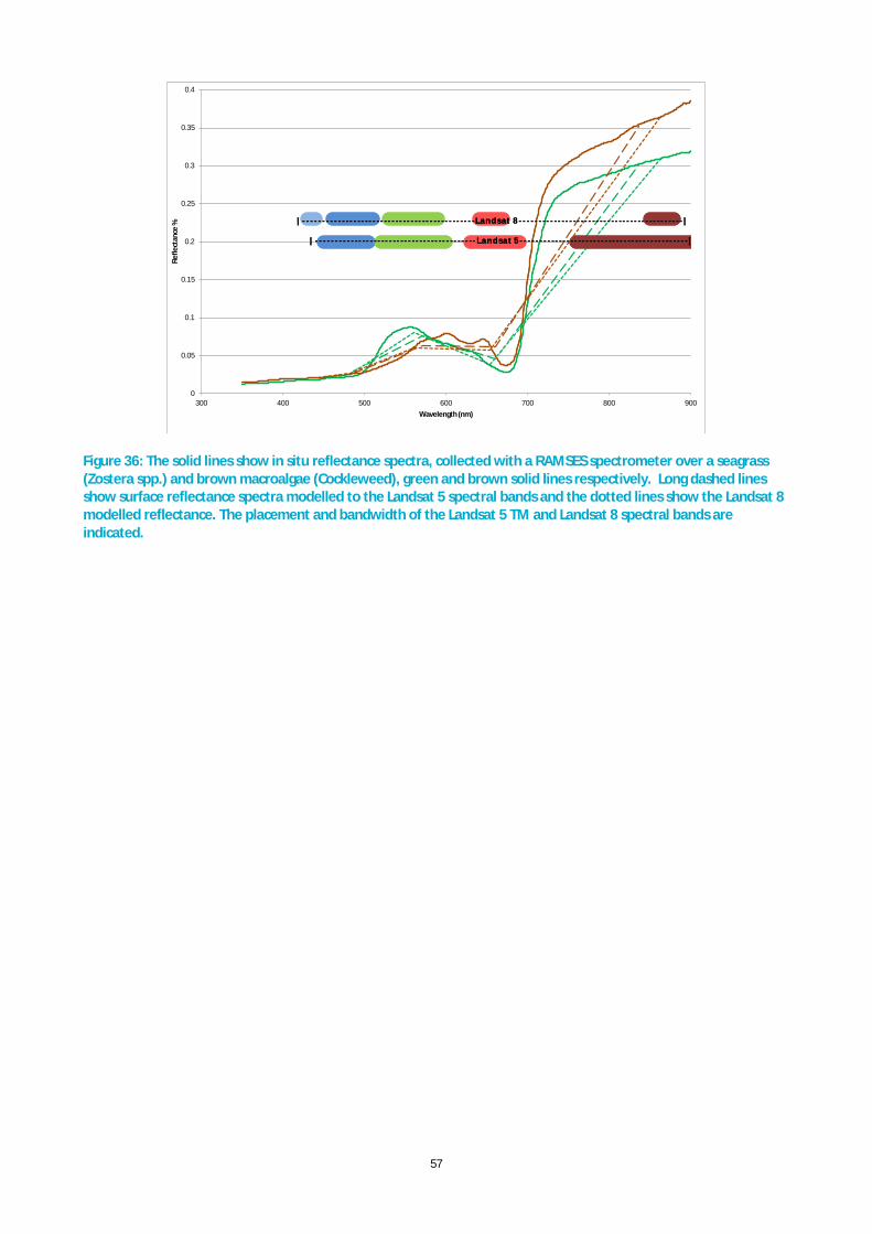
57

Figure 36: The solid lines show in situ reflectance spectra, collected with a RAMSES spectrometer over a seagrass (Zostera spp.) and brown macroalgae (Cockleweed), green and brown solid lines respectively. Long dashed lines show surface reflectance spectra modelled to the Landsat 5 spectral bands and the dotted lines show the Landsat 8 modelled reflectance. The placement and bandwidth of the Landsat 5 TM and Landsat 8 spectral bands are indicated.

0

0.05

0.1

0.15

0.2

0.25

0.3

0.35

0.4

300 400 500 600 700 800 900

Refle

ctan

ce %

Wavelength (nm)

| - - - - - - - - - - - - - - - - - - - - - - - - - - - - - - - - - - - - - - - - - - - - -L a n d s a t 8 - - - - - - - - - - - - - - - - - - - - - - - - - - - - - - - - - - - - - - - - - - - |

| - - - - - - - - - - - - - - - - - - - - - - - - - - - - - - - - - - - - - - - - - - L a n d s a t 5 - - - - - - - - - - - - - - - - - - - - - - - - - - - - - - - - - - - - - - - - - - - -|

| - - - - - - - - - - - - - - - - - - - - - - - - - - - - - - - - - - - - - - - - - - - - -L a n d s a t 8 - - - - - - - - - - - - - - - - - - - - - - - - - - - - - - - - - - - - - - - - - - - |

| - - - - - - - - - - - - - - - - - - - - - - - - - - - - - - - - - - - - - - - - - - L a n d s a t 5 - - - - - - - - - - - - - - - - - - - - - - - - - - - - - - - - - - - - - - - - - - - -|

58

Figure 37. Spectral characteristics of Landsat TM/ETM+ (top) and Landsat 8 (lower) overlaid on 4 common seagrass species spectra found in Western Port Bay.

5.1.5 CALIBRATION AND VALIDATION DATA

Macrophyte cover

The baseline maps required to both parameterise and validate modelling and the satellite-derived products were compiled for habitat (Table 9) and water quality information (Table 7).

Previous field surveys have found a high proportion of heterogeneity of the seagrass and macroalgal species within Western Port Bay. In Blake and Ball (2001), four species of seagrass were recorded: Zostera muelleri, Heterozostera tasmanica, Halophila australis and Amphibolis antarctica. The 155 km2 of seagrass and macroalgae they recorded were comprised of:

• 130 km2 of seagrass or a mixture of seagrass and algae.

• 45 km2 was the mixed category 'Dense Zostera/Heterozostera with algae'

• 20km2 was the mixed 'Amphibolis with Macroalgae‘

• 25km2 was 'Undefined Algae’

Field observation data from the Stephens (1995) and Blake and Ball (2001) reports were converted into GIS format (Figure 38 & Figure 39 respectively). The observation data used were collected from 26 July 1999 until 19 April 2000 and therefore highly appropriate for the 10 April 1999 Landsat 5 image’s validation. The in situ parameters recorded were date, location, species and density of cover.

0.00

0.10

0.20

0.30

0.40

0.50

0.60

400 500 600 700 800 900

Refle

ctan

ce %

Wavelength (nm)

Posidonia australis

Heterozoster tasmanica

Amphibolis antartica

Landsat TM bands

Zostera muelleri

0.00

0.10

0.20

0.30

0.40

0.50

0.60

400 500 600 700 800 900

Refle

ctan

ce %

Wavelength (nm)

Landsat 8 bands

Posidonia australis

Heterozoster tasmanica

Amphibolis antartica

Zostera muelleri

59

Table 9. Habitat baseline data and maps

DATA DATES SOURCE

Seagrass Map - Western Port Bay 1973-4 Bulthuis (1981)

Seagrass Map - Western Port Bay 1983-2 Bulthuis (1983b, 1984)

Seagrass Map - Western Port Bay 1994 Stephens (1995)

Seagrass Map – Western Port Bay 1999-2009 Blake and Ball (2001)

Seagrass Map – Yaringa and French Island Marine NP 2011 French et al. (2014)

Seagrass density - 3 sites in Western Port Bay 1980-1982 Bulthuis & Woelkerling (1983)

Rogers, Saintalan, & Heijnis (2005)

Shepherd, et al.(2009)

Seagrass Point measurements 2013-2014 Monash University – Rachel Manassa and Perran Cook

Figure 38. Seagrass map derived from Stephens (1995).

60

Figure 39. Seagrass map derived from Blake and Ball (2001)

Water Quality

The SAMBUCA retrieved NAP values within three Western Port segments were compared with the EPA TSS measurements in those segments. The Landsat SAMBUCA retrieval sites for Corinella and Barrallier Island were slightly offset from the EPA as shown, to ensure the retrievals were not affected by exposure at low tide. The Hastings retrieval site was coincident with the EPA location. USGS data was retrieved for the 3 locations whereas AGDC data was only retrieved from the Corinella and Barrallier sites.

Figure 40: Site locations of Landsat water quality time-series which were compared with the EPA sites 709 (Hastings), 716 (Barrallier) and 724 (Corinella).

61

5.2 Results

5.2.1 MACROPHYTE COVER

Preliminary substrate classification using Landsat MSS data

The oldest suitable Landsat MSS image available was acquired on the 19 January 1973. It was classified using standard maximum likelihood classifier, then compared with the 1973-4 maps in Bulthuis (1981). The image was acquired at high tide and much of the macrophyte coverage mapped in Bulthuis (1981) is submerged. The macrophytes can be seen submerged through the bay, and have some visibility in the near infrared bands in the intertidal region (Figure 41).

A Landsat 3 (MSS image) from 19 March 1979 (Figure 42) was also processed using the same technique as the 19 January 1973 image. This image shows less macrophyte coverage that mapped in Figure 41. The macrophytes can be seen submerged through the bay, and have some visibility in the near infrared bands in the intertidal region. There is more turbid water limiting the substrate visibility, particularly in the north east and south eastern portions of the bay.

Figure 41 Classification of the Landsat MSS image from 19 January 1973. This classification was labelled using Bulthuis, 1974.

62

Figure 42 Classification of the Landsat MSS image from 19 March 1979. This classification was labelled using the Bulthuis, 1974 map. Diagonal lines in the classification are coherent noise.

SAMBUCA substrate classification using Landsat 5 and 8 data

SAMBUCA was sensitive to the initial boundary conditions, that is, the starting value and range of the variables. A series of SAMBUCA tests were run using as input the two substrate (dark mud and bright sand) spectral libraries with the SAMBUCA-derived bathymetry estimate being then evaluated with the approximated depth measurements. An accurate bathymetry layer provided proved to be extremely valuable to constrain the model.

The best performing set of variables used in the parameterisation were used to constrain another SAMBUCA run using a 3 substrate library using a brown macroalgae, seagrass and sand spectra as possible substrates. The classes in the following Figures do not necessary indicate the full extent of the vegetation, only the retrieved vegetation after the quality control mask was applied.

Each pixel of the Landsat imagery is 30 by 30 meters, covering 900m2, therefore each pixel contains a ‘mixture’ of the reflectance of all the substrates within that 900m2. Together with this spatial heterogeneity, the broad bands of the Landsat sensor made it difficult to distinguish between macroalgae and seagrass spectra.

The images were at varying tide stages and were generally of good to high quality, with the SAMBUCA model predicting at least the combined extent of submerged seagrass and macroalgae:

· 11 April 1988 Landsat 5 image: This high quality image was acquired at low tide with significant macrophyte coverage visible (Figure 43). A smoke plume occurred at the time of acquisition over a small portion of the water on the south west of French Island but it did not appear to cover any submerged macrophytes. The plume and the plume shadow were removed prior to analysis.

· 29 December 1990 Landsat 5 image: This high quality image was acquired at a lower tide with significant macrophyte coverage visible.

· 21 October 1994 Landsat 5 image: This good quality image was obtained at a very low tide with significant macrophyte coverage visible.

· 31 October 1998 Landsat 5 image: This high quality image was acquired at low tide with significant macrophyte coverage visible. Significant systematic sensor noise doesn’t seem to impede the SAMBUCA retrieval, partially because the macrophyte cover is very visible due to high water clarity.

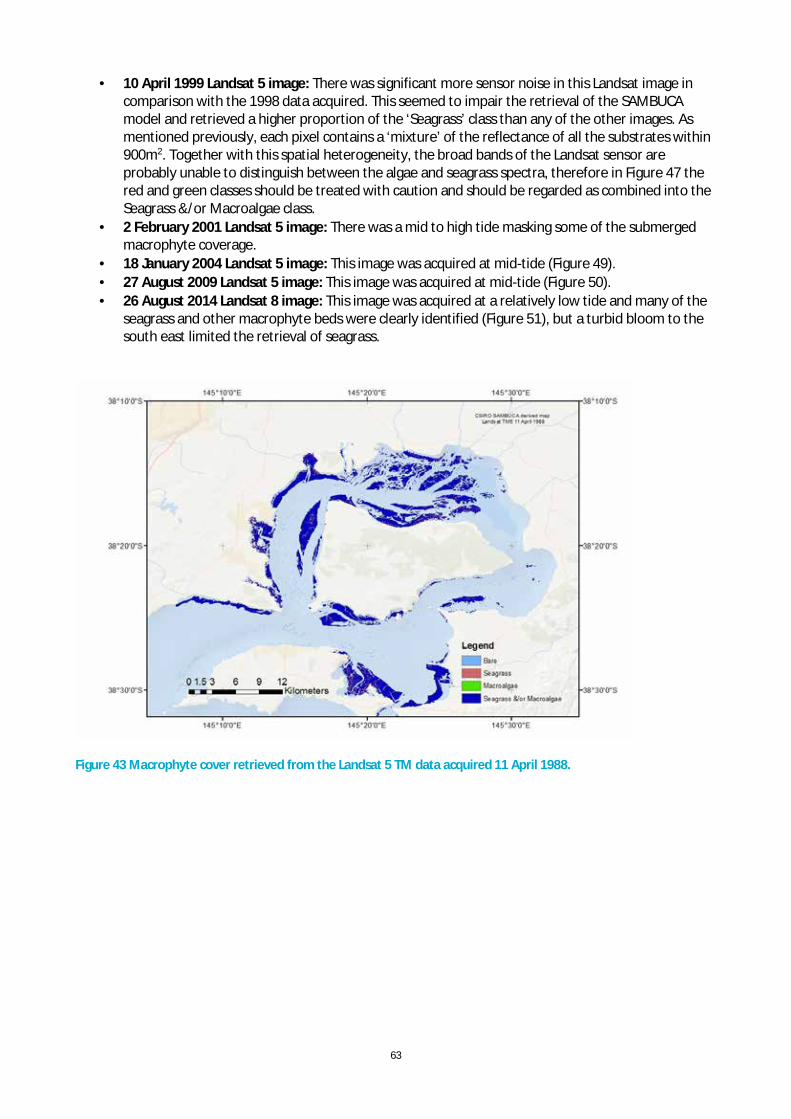
63

· 10 April 1999 Landsat 5 image: There was significant more sensor noise in this Landsat image in comparison with the 1998 data acquired. This seemed to impair the retrieval of the SAMBUCA model and retrieved a higher proportion of the ‘Seagrass’ class than any of the other images. As mentioned previously, each pixel contains a ‘mixture’ of the reflectance of all the substrates within 900m2. Together with this spatial heterogeneity, the broad bands of the Landsat sensor are probably unable to distinguish between the algae and seagrass spectra, therefore in Figure 47 the red and green classes should be treated with caution and should be regarded as combined into the Seagrass &/or Macroalgae class.

· 2 February 2001 Landsat 5 image: There was a mid to high tide masking some of the submerged macrophyte coverage.

· 18 January 2004 Landsat 5 image: This image was acquired at mid-tide (Figure 49). · 27 August 2009 Landsat 5 image: This image was acquired at mid-tide (Figure 50). · 26 August 2014 Landsat 8 image: This image was acquired at a relatively low tide and many of the

seagrass and other macrophyte beds were clearly identified (Figure 51), but a turbid bloom to the south east limited the retrieval of seagrass.

Figure 43 Macrophyte cover retrieved from the Landsat 5 TM data acquired 11 April 1988.

64

Figure 44 Macrophyte cover retrieved from the Landsat 5 TM data acquired 29 December 1990.

Figure 45 Macrophyte cover retrieved from the Landsat 5 TM data acquired 21 October 1994.

65

Figure 46 Macrophyte cover retrieved from the Landsat 5 TM data acquired 31 October 1998.

Figure 47: Macrophyte cover retrieved from the Landsat 5 TM data acquired 10 April 1999.

66

Figure 48: Macrophyte cover retrieved from the Landsat 5 TM data acquired 2 February 2001.

Figure 49: Macrophyte cover retrieved from the Landsat 5 TM data acquired 18 January 2004.

67

Figure 50: The Landsat 5 image of Western Port Bay from 27 August 2009.

Figure 51 : Macrophyte cover retrieved from the Landsat 8 data acquired 26 August 2014.

Time-series of macrophyte cover

The above maps indicates that there has been loss of macrophyte area between 1973 and the 1990’s, with a recovery in the mid to late 1990’s and then a gradual decline until 2014 (Figure 52). There is some likelihood that such changes may have occurred. However, the magnitudes of apparent changes in areal extent must be interpreted with caution because each image is at a different tidal state. The area over which macrophyte cover which can be retrieved by the SAMBUCA model in each image is sensitive to the tidal state for two reasons; firstly the area which is optically deep (which means the model cannot

68

distinguish reflectance from the substratum) varies with water depth, and secondly, the model functions only on the area covered by water and excludes intertidal areas exposed to the air at low tide. For example, the 2004, 2009 and 2014 images are all acquired at a low tidal state. The comparable macrophyte cover between these images indicates some stability during these years, but may exclude some cover in additional intertidal areas.

If seagrass loss is to be assessed in Western Port temporally, then this should be assessed for the whole bay. Naturally, most seagrasses tend to die off over time and recolonise in other areas, therefore it is the scale of change that is important, rather than the exact locations. This research has identified that a hybrid modelling approach should be considered to enable comparison of macrophyte extent between dates and tide stages, including both submerged areas and exposed intertidal areas. This approach would involve combining SAMBUCA retrievals with a physically-based model designed for exposed intertidal areas. Reporting the optically-deep area which could not be assessed will also be important for developing standard monitoring products.

The Western Port Environmental study (Sharpio, 1974), documented about 400 km2 of coastal, shallow-water seagrass habitat in Western Port. While this corresponds well with analysis of the Landsat image in 1973 (Figure 52), which was taken at high tide, suggesting that when water clarity is good and tide stage is high, Landsat imagery can be used to assess the areas of seagrass and bare substrate. Further, the model validation against subsequent seagrass mapping (below) indicates that the combined extent of seagrass and macroalgae can be predicted well.

Figure 52: The areal extent of benthic cover estimated by SAMBUCA from the Landsat time series (at various tidal states). Data labels are the total area assessed at each date in square kilometres. A maximum likelihood classification was used for the 1973 and 1979 data and the SAMBUCA method was used for subsequent years. The ‘seagrass’, ‘macroalgae’, and ‘seagrass &/or macroalgae’ classes were combined.

Validation of macrophyte cover

Validation data for satellite thematic maps require a spatially dense sampling design along transects and homogenous features. The in situ observations collected for the validation are independent of the SAMBUCA predicted substrate class in the thematic maps. The image-derived benthic cover maps (Figure 43-Figure 51) shows the presence of two pure vegetation substrate types as well as a mixed class where a combination of any two out of three substrate types is present in the pixel.

Accuracy of the Western Port SAMBUCA substrate retrievals were assessed using (Stephens, 1995 and Blake and Ball, 2001) field data collected in 1994 (Figure 38) and 1998 (Figure 47). As previously discussed Landsat data, due to its spectral resolution, has limited ability to separate species such seagrass from algae,

62.8

114.7

11.6 1.241.4

9.6

114.1

65.017.3 15.4

345.0

161.6

319.6

263.3

338.9

474.9 249.9

215.9

213.4 212.7

0

100

200

300

400

500

600

1973 1979 1988 1990 1994 1998 2001 2004 2009 2014

Area

(km

2)

bare macrophyte

69

therefore the SAMBUCA substrate retrievals were also assessed after combining the seagrass and algae classes (Table 15).

The accuracy assessment is presented in confusion matrix format (Table 10 - Table 14). Each row of the table represents the satellite-derived classes and each column displays the corresponding ground truth classes in the identical order. Overall accuracy is calculated by dividing the total number of pixels that were correctly classified, i.e. assigned to the correct class, by the total number of validation pixels or reference points used to construct the error matrix (Congalton, 1991). Although the overall accuracy is the most commonly used accuracy measure, it does not take into account both errors of commission and omission for all individual classes.

The producer accuracy is the probability of a reference data point being classified correctly, whereas the user accuracy is the probability of a classified pixel being correct. The user and producer accuracies determine where misclassification has occurred, and where pixels have been erroneously excluded (omission), or included (commission), in an image class. The producer accuracy for a particular class is calculated for each column by dividing the number of correctly identified class pixels by the column total pixels. The user accuracy is calculated for a class by dividing the number of correctly identified class pixels by the row total pixels.

The conditional kappa coefficient (maximum value =1) reports the statistical measure of the extent to which the classification is a correct representation of the field data. The kappa coefficient is a measure of the improvement by a classifier compared to a purely random assignment of classes. The higher the kappa coefficient value, the closer the agreement.

Validation of the 1994 Landsat data was undertaken using the Stephens (1995) data which was categorised into 4 classes: land, dense, moderate or sparse seagrass. There were no macroalgae classes or bare substrates recorded in the data provided. For comparison, the ‘dense seagrass’ was compared with the SAMBUCA retrieved ‘Seagrass &/or Macroalgae’ class; the ‘moderate seagrass’ was compared with the SAMBUCA ‘Macroalgae’ class; the ‘sparse seagrass’ was compared with the SAMBUCA ‘Seagrass’ class, and finally the ‘Land’ class was compared with the SAMBUCA ‘Bare’ class (Table 10). The Stephens classes are distributed through the confusion matrix, with the majority of the seagrass mapping in the SAMBUCA combined Seagrass &/or Macroalgae class, and a low overall accuracy of 10% is achieved. When the macrophytes (‘Seagrass’, ‘Macroalgae’ and ‘Seagrass &/or Macroalgae’) classes are combined the overall accuracy improves to 65%.

Using the Blake and Ball (2001) field data, the 1999 Landsat image was also assessed for accuracy. The noise of that image impacted the SAMBUCA retrieval in comparison with the 1998 Landsat image. The overall accuracy for the 4 classes was 16% for the 1999 image compared to 53% for the 1998 image. When combining the macrophyte classes the accuracy improved significantly to 95% for the 1999 compared with 85% for the 1998 image, indicating the noise in the 1999 image impacted the discrimination between the substrate classes much more than the other images. The 1999 image was therefore disregarded in subsequent analysis.

70

Table 10: The pixel accuracy assessment of the 1994 Landsat SAMBUCA retrieved substrates when compare with the Stephens (1995) field data collected during 1994. The overall accuracy is low at 10%, with a kappa co-efficient of -0.0163.

SAMBUCA substrate retrieval Stephens (1994) data

PIXELS Unclassified Bare Seagrass Macroalgae Mix Seagrass/Algae

Row Total

Users Accuracy %

Land 389 2 3 3 40 437 1.12 Sparse Seagrass

7663 52 1513 1102 15787 26117 41.28

Moderate Seagrass

12656 77 1752 1142 21588 37215 46.84

Dense Seagrass

5284 47 397 191 4918 10837 11.62

Column Total 25992 178 3665 2438 42333 74606 Producers Accuracy %

0.46 5.76 3.07 45.38

Table 11: The pixel accuracy assessment of the 1994 Landsat SAMBUCA retrieved substrates when compare with the combined algae and seagrass classes from the Stephens (1995) field data collected during 1994. The overall accuracy is 65%, with a kappa coefficient at 0.0092.

SAMBUCA substrate retrieval Stephens (1994) data

PIXELS Unclassified Mix Seagrass/Algae

Bare Row Total Users Accuracy %

Seagrass 25209 47674 176 73059 99.9 Land 389 46 2 437 1.12 Column Total 25598 47720 178 73496 Producers Accuracy %

65.25 0.46

Table 12: The pixel accuracy assessment of the 1998 Landsat SAMBUCA retrieved substrates when compare with the Blake and Ball (2001) field data collected during 1999. The overall accuracy is low at 52%, with a kappa co-efficient of 0.0384.

SAMBUCA substrate retrieval Blake and Ball (2001) data

PIXELS Unclassified Mix Seagrass/Algae

Bare Macroalgae Seagrass Row Total

Users Accuracy %

Mix Seagrass/Algae

7217 87272 336 1874 7555 104254 61.56

Bare 1300 7730 126 348 756 10260 22.66 Macroalgae 2418 23875 47 478 1820 28638 15.74 Seagrass 5513 22886 47 336 2908 31690 22.30 Column Total 16448 141763 556 3036 13039 174842 Producers Accuracy %

83.1 1.23 1.67 9.18

71

Table 13: The pixel accuracy assessment of the 1998 Landsat SAMBUCA retrieved substrates when compare with the combined algae and seagrass classes from the Blake and Ball (2001) field data collected during 1999. The overall accuracy is 85%, with a kappa coefficient at 0.0199.

SAMBUCA substrate retrieval

Blake and Ball (2001) data

PIXELS Unclassified Mix Seagrass/Algae

Bare Row Total Users Accuracy %

Mix Seagrass/Algae

15113 148652 426 164191 94.39

Bare 1300 8841 126 10267 22.83

Column Total 16413 157493 552 174458

Producers Accuracy %

90.54 22.83

Table 14: The pixel accuracy assessment of the 1999 Landsat SAMBUCA retrieved substrates when compare with the Blake and Ball (2001) field data collected during 1999. The overall accuracy is low at 16%, with a kappa co-efficient of 0.0121.

SAMBUCA substrate retrieval Blake and Ball (2001) data

PIXELS Mix Seagrass/Algae

Seagrass Algae Bare Row Total Users Accuracy

Mix Seagrass/Algae 0 0 0 0 7821 0.0 Seagrass 4481 1437 1348 555 11223 0.18 Algae 6788 1342 1689 1404 369 0.15 Bare 0 0 0 0 101 0.00 Column Total 11269 2779 3037 1959 19044 Producers Accuracy 0.0 0.52 0.56 0.00

Table 15: The pixel accuracy assessment of the 1999 Landsat SAMBUCA retrieved substrates when compare with the combined algae and seagrass classes from the Blake and Ball (2001) field data collected during 1999. The overall accuracy is 95%, with a kappa coefficient at 0.752.

SAMBUCA substrate retrieval

Blake and Ball (2001) data

PIXELS Mix Seagrass/Algae

Bare Unclassified Row Total Users Accuracy

Mix Seagrass/Algae

131637 7248 0 138885 0.95

Bare 12240 791 44118 57149 0.01

Unclassified 17230 1921 1469647 1488798 0.99

Column Total 161107 9960 1513765 1684832

Producers Accuracy

0.82 0.08 0.97

72

5.2.2 WATER QUALITY RESULTS

Non-Algal Particulate Concentration

Monthly river TSS loads were compared with a time-series of non-algal particulate matter (NAP) derived from Landsat remote sensing images for the Corinella segment (Figure 53). While NAP was variable, probably influenced by wind and tides, the annual minimum NAP concentrations tended to be higher in years following monthly river TSS loads greater than ~5 kt (Figure 53). NAP annual-minimum concentrations were much lower (<2 mg L-1) during 2001–2012 when monthly loads were generally <5 kt. This analysis indicates that high catchment TSS inputs result in more chronically turbid conditions in the Corinella segment of Western Port, and that lower NAP concentrations are much more likely to occur when TSS inputs remain low for extended periods (e.g., during El Nino periods). This may indicate that sediment resuspension from the Upper North Arm declines after a year or more of low catchment inputs. A similar phenomenon is observed offshore from the Burdekin River in the central Great Barrier Reef lagoon, where water clarity is initially reduced following large river flow events, which are known to deliver large TSS and nutrient loads, but then gradually recovers over several months (Fabricius et al., 2014).

Figure 53: Monthly river TSS loads summed across the four stream gauges (from Section 2.3.2) compared with the time series of non-algal particulate concentrations from Landsat SAMBUCA modelling in the Corinella segment of Western Port.

There was substantial spatial variation in estimated NAP within each image, and between adjacent images over 26 years (Figure 54). These variations can be related to the tide stage and range, and the wind-driven wave climate. In particular, high turbidity was generally associated with high winds (wind speed is described using the Beaufort scale), and tide stage and range had variable effects in different parts of the bay:

· 11 April 1988 Landsat 5 image: High turbidity was retrieved at high tide and large tide range, with high wind trending from the north-east in the preceding 12 hours and a moderate breeze at the time of acquisition.

· 29 December 1990 Landsat 5 image: Low turbidity was retrieved at high incoming tide, with a moderate breeze from the north-west in the preceding 12 hours and dropping to a light breeze from the north-east at the time of acquisition.

· 21 October 1994 Landsat 5 image: High turbidity was retrieved at high outgoing tide, with a fresh breeze from the south-east in the preceding 12 hours and changing direction to the north-east at the same wind speed time of acquisition.

73

· 31 October 1998 Landsat 5 image: Low turbidity was retrieved at low tide, with a moderate breeze from the south-west in the preceding 12 hours and dropping to a fresh breeze at the time of acquisition.

· 2 February 2001 Landsat 5 image: High turbidity was retrieved at high tide, with a light breeze from the west in the preceding 12 hours and changing to a moderate breeze from the north-east at the time of acquisition.

· 18 January 2004 Landsat 5 image: High turbidity was retrieved at the middle of the tide, with a high winds from the south-west in the preceding 12 hours and changing to a fresh breeze from the north-east at the time of acquisition.

· 27 August 2009 Landsat 5 image: High turbidity was retrieved at low incoming tide, with a storm winds from the north-west in the preceding 12 hours and changing to gale winds also from the north-east at the time of acquisition.

· 20 June 2013 Landsat 8 image: High turbidity was retrieved at low incoming tide, with a light breeze from the south-west in the preceding 12 hours and changing to a gentle breeze from the north at the time of acquisition.

· 26 August 2014 Landsat 8 image: High turbidity was retrieved at low outgoing tide, with a gentle breeze from the south-west in the preceding 12 hours and changing to a light breeze from the north-west at the time of acquisition.

Analysis of remotely sensed multi-decadal time-series data such as this has the potential to augment the in situ total suspended matter measurement records to provide a fuller understanding of the spatial and temporal dynamics of water quality within Western Port.

74

-0.2

-0.1

0

0.1

0.2

0.3

0.4

0.5

0.6

0.7

0.8

tide

heig

ht (m

)

-0.4

-0.2

0

0.2

0.4

0.6

0.8

1

tide

heig

ht (m

)

East Sale Wind Direction

Wind Speed (ms-1)

-12 hours 55 15.4

Time of Acquisition

45 7.2

+12 hours 275 6.1

East Sale Wind Direction

Wind Speed (ms-1)

-12 hours 300 7.2

Time of Acquisition

35 3.0

+12 hours 290 10.3

0

0.1

0.2

0.3

0.4

0.5

0.6

0.7

0.8

0.9

tide

heig

ht (m

)

0

0.1

0.2

0.3

0.4

0.5

0.6

0.7

tide

heig

ht (m

)

East Sale Wind Direction

Wind Speed (ms-1)

-12 hours 140 9.2

Time of Acquisition

70 9.2

+12 hours 70 7.2

East Sale Wind Direction

Wind Speed (ms-1)

-12 hours 220 12.3

Time of Acquisition

210 9.7

+12 hours 175 8.7

0

0.1

0.2

0.3

0.4

0.5

0.6

tide

heig

ht (m

)

East Sale Wind Direction

Wind Speed (ms-1)

-12 hours 265 2.6

Time of Acquisition

45 7.7

+12 hours 330 5.1

75

Figure 54. Maps of non-algal particulate (NAP) concentration from the SAMBUCA model, based on the same Landsat 5, 7 & 8 images for which seagrass and macro-algae were predicted (from 11 April 1988 top left until 26 August 2014, bottom right). Higher concentrations are shown in blue, intermediate concentrations in green and lower concentrations in red. The historical tide height estimates were obtained using WXTide32 (http://www.wxtide32.com/index.html), developed by the National Ocean Service (U.S.A.), and are not validated.

Validation of concentration estimates

There was some variation between the SAMBUCA estimates based on the USGS and AGDC Landsat archives, while the EPA measurements were generally between these two predictions (Figures 48-50).

-0.4

-0.2

0

0.2

0.4

0.6

0.8

tide

heig

ht (m

)

0

0.1

0.2

0.3

0.4

0.5

0.6

0.7

0.8

0.9

tide

heig

ht (m

)

East Sale Wind Direction

Wind Speed (ms-1)

-12 hours 285 28.8

Time of Acquisition

290 19.0

+12 hours 190 15.9

East Sale Wind Direction

Wind Speed (ms-1)

-12 hours 240 16.5

Time of Acquisition

220 10.3

+12 hours 240 5.7

0

0.1

0.2

0.3

0.4

0.5

0.6

0.7

0.8

0.9

tide

heig

ht (m

)

-0.2

-0.1

0

0.1

0.2

0.3

0.4

0.5

0.6

0.7

0.8

0.9

tide

heig

ht (m

)

East Sale Wind Direction

Wind Speed (ms-1)

-12 hours 225 3.6

Time of Acquisition

280 2.1

+12 hours 305 3.6

East Sale Wind Direction

Wind Speed (ms-1)

-12 hours 225 2.6

Time of Acquisition

355 3.6

+12 hours 0 5.7

76

Figure 55: SAMBUCA retrieval of non-algal particulates (NAP) concentration from the USGS images (circles), and from the AGDC (triangles) in the Corinella segment, compared with TSS measurements at the EPA Corinella site (squares).

Figure 56: SAMBUCA retrieval of non-algal particulates (NAP) concentration from the USGS images (circles), and from the AGDC (triangles) in the Upper North Arm, compared with TSS measurements at the EPA Barrallier Island site.

Figure 57: SAMBUCA retrieval of non-algal particulates (NAP) concentration in the Lower North Arm segment from the USGS images (circles), compared with TSS measurements at the EPA Hastings site (squares). No AGDC retrievals were undertaken for this site.

0

5

10

15

20

25

30

35

40

NAP

or T

SS m

g/L

Corinella_NAP Corinella_EPA_TSS AGDC SAMBUCA NAP

0

10

20

30

40

50

60

70

80

90

NAP

or T

SS g

/L

Barrallier Is_NAP Barrallier_EPA_TSS AGDC_SAMBUCA_NAP

0

5

10

15

20

25

30

NAP

or T

SS m

g/L

Hastings_NAP Hastings_EPA_TSS

77

Differences between the USGS and AGDC data are attributed to differences in atmospheric corrections applied to the raw imagery. The blue green and red bands from each of the algorithms show a general agreement but some scatter (Figure 58), which explains the differences in SAMBUCA retrievals from the two datasets.

Figure 58: The comparison between the surface reflectance products produced by the AGDC (y-axis) and the USGS (x-axis) for the blue, green and red bands.

The AGDC data uses a nadir Bi-directional Reflectance Distribution Function to adjust the reflectance. The output from the model is surface reflectance standardised to a fixed viewing and illumination geometry. The model has been parameterised for eastern Australia, but has been applied to the whole of Australia.

The USGS Landsat 4, 5 and 7 data are generated from the Landsat Ecosystem Disturbance Adaptive Processing System (LEDAPs) which applies a MODIS atmospheric correction to the level 1 data, then is rerun using the Second Simulation of a Satellite Signal in the Solar Spectrum (6S) radiative transfer model to obtain surface reflectance and other outputs.

The USGS Landsat 8 data are generated from the Landsat Surface Reflectance Code (LaSRC) which uses the coastal aerosol band to estimate aerosol thickness then using additional auxiliary climate data from MODIS as input parameters, runs an in-built radiative transfer code to calculate surface reflectance and other outputs.

Vertical Diffuse Attenuation Coefficient (Kd)

The SAMBUCA retrieved Kd(490)nm values (from USGS data) are plotted with the EPA Kd(PAR) values obtained in the same 3 EPA sampling sites (Figure 59 - Figure 61) at Corinella, Barrallier Island and Hastings. Without developing a similar relationship between the Kd(490)nm and Kd(PAR) metrics (which requires field measurement), the results cannot be directly comparable, but if the relationship between the Kd(490)nm and Kd(PAR) is consistent with previous published studies, it indicates a reasonable SAMBUCA result. The remote sensing extends the monitoring record substantially. The spatial extent of Kd(490)nm retrieved from the Landsat USGS archive is shown in Figure 62.

USGS Landsat 8 band 2 (Blue)

AGDC

Lan

dsat

8 b

and

2 (B

lue)

USGS Landsat 8 band 2 (Green)AG

DC L

ands

at 8

ban

d 2

(Gre

en)

AGDC

Lan

dsat

8 b

and

2 (R

ed)

USGS Landsat 8 band 2 (Red)

78

Figure 59: The SAMBUCA retrieved Kd (490nm) from USGS data (circles) compared with the EPA Kd (squares) as calculated from PAR measurements at the EPA Corinella sampling location (EPA measurements from Holland et al., 2013).

Figure 60: The SAMBUCA retrieved Kd (490nm) from USGS data (circles) compared with the EPA Kd (squares) as calculated from PAR measurements at the EPA Barrallier Island sampling location (EPA measurements from Holland et al., 2013).

Figure 61: The SAMBUCA retrieved Kd (490nm) from USGS data (circles) compared with the EPA Kd (squares) as calculated from PAR measurements at the EPA Hastings sampling location (EPA measurements from Holland et al., 2013).

79

Figure 62: The SAMBUCA retrievals for Kd (490 nm) from the USGS Landsat 5, 7 & 8 images acquired from 11 April 1988 top left until 26 August 2014, bottom right. Low Kd (490nm) values (shown in red) indicating increased water clarity and light availability at the seafloor.

MODIS Aqua Kd (490nm) products are derived from the NASA MODIS Terra and Aqua satellites that were launched in 1999 (Terra) and 2002 (Aqua). The mean Kd (490nm) are plotted from CSIRO Oceans Remote Sensing ERDDAP which provides access to CSIRO and Integrated Marine Observing System (IMOS) Ocean Remote Sensing data (http://rs-data2-mel.csiro.au/erddap).

A polygon encompassing the area analysed by the Landsat area was interrogated in ERDDAP for mean values of Kd 490nm (Figure 63).These are monthly composites of 1km data for Australia. This data indicates reasonably stable conditions between 2002 and 2010, then an increase of Kd values between 2010 and 2014. A marked change in conditions is seen in the MODIS data from the start of 2015 in both amplitude and range. From the start of 2015, the coastal mask used increased the density of data points which can be seen in Figure 64.

The MODIS data Kd values consistently range between 0.3-0.7 m-1 whereas the EPA Kd(PAR) and USGS SAMBUCA retrieved Kd 490nm values both have higher variability between 0.3-2.2 m-1. The variability between the MODIS data and the EPA and satellite retrieved results are as a result of the differences between the spatial and spectral resolution of the sensors (eg MODIS data is 1km versus Landsat is 30m and 8 bands are used for MODIS vs Landsat’s 4), and the global algorithms used in MODIS products. In Western Port, it is probable that the large pixel size of MODIS has resulted in contamination by the substrate. The MODIS algorithm calculates the Kd 490nm values using an empirical relationship derived from in situ measurements of Kd490nm and blue-to-green band ratios of remote sensing reflectances (Rrs). However, the MODIS models are generally applicable for clear open ocean waters. In Wang et al, (2009) , their results show that Kd 490nm results for the Chesapeake Bay are significantly underestimated by a

80

factor of 2–3 compared with the in situ data. The SAMBUCA algorithm accounts for the substrate in the retrieval of the Kd 490nm (and other water quality parameters).

Figure 63: MODIS Aqua mean values for Kd 490 nm (grey) from whole of the Western Port Bay area from July 2002 until September 2015 within the region specified by the polygon, top left:38.20°S,145.11°E and lower right 38.53°S, 145.57°E. This data is available in a tabular format with geographic reference and date. The MODIS data is compared with the Landsat SAMBUCA retrieved Kd (490nm) as circles compared with the EPA Kd as squares as calculated from PAR measurements at the EPA Hastings sampling location (EPA measurements from Holland et al., 2013).

0

0.5

1

1.5

2

2.5

Kd m

-1

Corinella_Kd490nm Barrilier Is_Kd490nm Hastings_Kd490nm Corinella_EPA_Kd(PAR)

Barrilier_EPA_Kd(PAR) Hastings_EPA_Kd(PAR) MODIS Kd(490) mean m-1

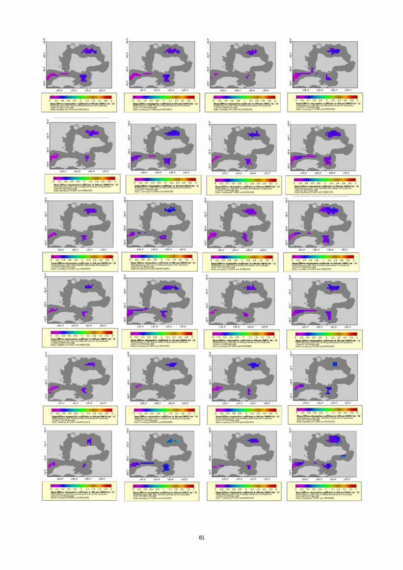
81

82

Figure 64: MODIS Aqua K_490 1km monthly time series for Australia, Dataset ID: csiro_1m_1km_aust_K_490.

All the maps and comparisons with in situ data presented in this report were produced using the SAMBUCA software which has been written in open source code will be made available in the future to the management and research community.

5.3 Gaps and Limitations

From this remote sensing processing we have identified several gaps or data limitations: · Model outputs are limited to the optically shallow portions of the images. Significant portions of

the Western Port Landsat scenes were covered with optically deep water, that is, where the substrate reflectance cannot be determined either from the confounding effects of the water column depth or because of the water clarity.

· The Landsat sensor lacks sufficient spectral sensitivity to distinguish between the spectral classes of seagrass and algae, unless it is in areas of significant homogeneity that encompass more than one Landsat pixel (625 m2 for AGDC or 900m2 for the USGS data). This was not highly significant as much of the validation data was also categorised with broad classes.

· Improved spectral and spatial resolution of new sensors will be required to monitor species below the broad categories previously used for monitoring. Additional integration of in situ data will assist in this process, but will require objective methodologies for comparison through time.

· Parameterisation of the water quality model was undertaken using values obtained in the literature but in situ measurement, preferably over a range of seasons, would improve the model predictions.

· The early 1970-1980 macrophyte maps from field survey by Bulthius (1981, 1983b & 1984) were not available in digital form but would further improve model predictions of macrophyte extent.

83

5.4 Conclusions

Retrieval of water quality information from satellite imagery can provide an improved understanding into the spatial and temporal variability of the water body for environmental and resource managers. Field-based observational data are usually highly accurate but are expensive and often do not represent the spatial and temporal dynamics of the system. This project has shown that satellite analyses have the ability to augment field-based observations of benthic cover and water quality. Currently multi-decadal Landsat data can be utilised for temporal analyses of water quality but require a standardised approach to ensure trend analyses are comparable. The advent of the AGDC allows the consistent processing of Landsat data to surface reflectance which enables the large-scale time series analysis of water quality dynamics.

The SAMBUCA model was used to map the macrophyte extent on the substratum of Western Port for 10 Landsat images; from 11 April 1988 until 26 August 2014. We conclude that this approach can distinguish non-vegetated substrate from macrophyte cover, but that the spectral resolution of Landsat was insufficient to separate seagrasses from macroalgae. Time-series analyses of the ‘macrophyte’ class indicates a decline between the early 1970’s and a recovery in the late 1990’s. From the peak in 1998, there is a decline in assessed coverage, with the lowest coverage assessed between 2009 and 2014. As the 2004, 2009 and 2014 images were acquired during low tide, it may mean this decline in macrophyte cover could be due to intertidal areas being exposed and so excluded from the SAMBUCA retrievals. This has highlighted the need for future monitoring by remote sensing to be based on a hybrid remote sensing approach, whereby exposed areas are also assessed using a standardised physics-based approach and incorporated with the SAMBUCA subtidal estimates of cover.

The modelling was also used to map non-algal particulate concentrations and light attenuation in the water column for the same 10 Landsat images. It is concluded that the NAP and Kd(490nm) maps offer a much more spatially comprehensive view of the complex bay environment, including the interactions of tides, winds, resuspension and delivery of sediment from the catchment.

More comprehensive time-series of non-algal particulate concentrations and light attenuation were developed at three locations corresponding to EPA in situ measurements of TSS (Corinella, Barrallier Island and Hastings). We conclude that there were periods of chronic turbidity which corresponded with periods where large river TSS loads occurred (Section 2.3.2). Therefore time series analysis of NAP retrievals can be used to determine historical trends of turbidity within the bay.

5.5 Future Directions

There exists opportunity to develop ongoing monitoring of the substrate and water quality by routinely applying the SAMBUCA model we have parameterised for Western Port to Landsat 8 imagery. Both the AGDC and USGS have incorporated the new Landsat 8 imagery into their data acquisitions. All the data have been pre-processed to a consistent geographic grid using LPGS Version LPGS 11.6.0, then follows an atmospheric correction (Li et al. 2010) and pixel quality flagging (Irish et al. 2006) procedure.

The improvements in the Landsat 8 OLI design provide an increased data capture capacity, radiometric resolution and better signal to noise performance compared to the older Landsat satellites, which has led to greater accuracy in water quality retrievals. An example of a recent image of Western Port Bay (Figure 65) shows the detail and resolution that can be acquired with the new Landsat 8 sensor.

The AGDC database is accessible on the NCI system (http://nci.org.au/), thereby leveraging the high-performance computing power of Australia’s most highly integrated supercomputer and filesystems. Querying and advanced retrieval of AGDC data occurs through a Python-based application programming interface (API), available as a loadable module on the NCI system. Future satellite sensors such as the Sentinel sensors will be incorporated into the AGDC and the tools developed as part of the project can be applied to these new data streams to continue the time series in a standardise manner.

84

Figure 65: A Landsat 8 image acquired on 25 April 2016 at very low tide. Significant macrophyte coverage is exposed on the intertidal flats and substrate visibility is possible in the majority of the bay. Although SAMBUCA would not be able to retrieve the emergent macrophytes, a standard spectral classification method would potentially be able to discriminate the substrate at a higher resolution.

The new Sentinel remote sensing satellites now provide imagery which can be used in SAMBUCA model developed for this Western Port Bay project, to derive substrate and water quality monitoring products at finer spatial and spectral resolution than Landsat. These satellites are operated by the European Space Agency (ESA) for the Copernicus programme. Each Sentinel mission is based on a constellation of two satellites to fulfil revisit and coverage requirements. These missions carry a range of technologies, such as radar and multi-spectral imaging instruments for land, ocean and atmospheric monitoring. The two missions relevant for coastal monitoring are Sentinel-1 and Sentinel-2:

· Sentinel-1 is a polar-orbiting, all-weather, day-and-night radar imaging mission for land and ocean services. Sentinel-1A was launched on 3 April 2014 and Sentinel-1B on 25 April 2016.

· Sentinel-2 is a polar-orbiting, multispectral high-resolution imaging mission for land monitoring to provide, for example, imagery of vegetation, soil and water cover, inland waterways and coastal areas. Sentinel-2 can also deliver information for emergency services. Sentinel-2A was launched on 23 June 2015 and Sentinel-2B will follow in the second half of 2016. A limited release of data is currently being made available through ESA. Sentinel-2A’s bandset is similar to the MERIS platform, but at a much higher spatial resolution (10m in visible bands), making it particularly useful in complex coastal waters such as Western Port.

A consortium between CSIRO, Geoscience Australia and other partners are developing a regional data hub to serve the Copernicus ‘analysis ready’ data to the Earth Observation (EO) community via the National Computing Infrastructure.

85

Recommended Follow-on Activities

Several activities are recommended based on the improved understanding of the Western Port Bay region gained from the Landsat analysis. Gaps in understanding need to be addressed particularly improving the bio-optical characterisation, which will enable on going remote sensing analyses and integration of new sensors such as the Sentinel-2 data. All the analyses have limited value by management authorities if the products are not presented in a manner that can be interpreted, compared and accessed by managers, making a data portal for this purpose increasingly important.

Activity 1: Develop a hybrid remote sensing approach to monitoring benthic cover across the tidal cycle: This would improve the reliability of historical and future monitoring by allowing use of imagery at a range of tide stages.

Activity 2: Bio-optical characterisation of Western Port Bay: This would acquire a full optical characterisation of Western Port Bay using in situ measurements over a range of macrophytes, tidal cycles and at high and low flow conditions, to support the accurate parameterisation for water quality and macrophyte detection. Measurements with well calibrated instruments would include subsurface down-welling and upwelling irradiance spectra, absorption spectra of particle and dissolved substances, as well as chlorophyll and total suspended matter concentrations.

Activity 3: Sentinel implementation for monitoring and modelling: This activity would implement Sentinel 2 data into the processing pathway developed for Landsat to derive macrophyte cover and water quality parameters in Western Port. It would involve applying inversion-based models (e.g., SAMBUCA) to Sentinel 2 data. Sentinel 2 offers high spatial resolution (10-20m) in the spectral domain 443–2190 nm, has a wide swath and frequent revisiting time, which makes it highly suitable for monitoring and inventorying purposes. Sentinel-2 will enhance the Landsat data archive.

Activity 4: Estimating particle size in coastal waters: This activity would apply a model of the size of suspended particulate matter to Western Port Bay turbid coastal waters, which could be used to identify river plumes and resuspension dynamics. It would involve:

· Investigate bio-optical relationships using in situ data. · Develop and calibrate a model that relates optical properties to particle size. · Apply the model to Landsat and Sentinel-2/3 reflectance data. · Decouple the bay resuspension from sediment delivery.

Activity 5: Visualisation Products: This would develop a data portal to provide access to all data products, models, in situ data and remote sensing products.

86

6 Seagrass modelling

6.1 Objectives

The objective of this activity was to integrate the main processes affecting seagrass growth into a model describing hydrodynamics, biogeochemistry and seagrass growth. Seagrass in Western Port is subject to a multitude of stressors, especially on the shallower intertidal banks. Beside changes in land-use and thus run-off to the bay and its associate impact on seagrass via sediment dynamics (de Boer 2007, Pedersen et al. 2012), climate change will alter the distribution of seagrass beds as well (Short and Neckles 1999).

Context

Seagrass extent, growth, and decline are driven by the hydrodynamics and water quality in the bay affecting the physical environment for growth, the underwater light climate, and the availability of sediments and nutrients. There is also a feedback from seagrass stands on the hydrodynamics, by their increased drag changing flow patterns, which then impacts on sediment transport and increases net sedimentation rates (Bos et al. 2007). Furthermore seagrass beds can reduce sediment resuspension by wind driven waves, with the consequent reduction in turbidity leading to a positive feedback of enhanced seagrass growth. Detailed studies of these interactions (e.g., Abdelrahman 2003) show that this process depends on factors like plant morphology or flow induced bending, but these factors are not part of the current study due to their complexity.

Here we focus on the development of a stand-alone seagrass model, which can be fitted into a larger 3D hydrodynamic-wave model run by Melbourne Water and Hydronumerics Pty Ltd. The hydrodynamic-biogeochemical model (ELCOM/CAEDYM) was implemented and run by Hydronumerics and Melbourne Water, which predicts the currents, transport and settling of sediment, as well as a range of biogeochemical variables in Western Port. The ELCOM/CAEDYM model suite is driven by local meteorology and sea level variations at the entrance, as well as river inflows, sediment and nutrient loads. Sediment induced effects on light limited growth are, to some extent already included in CAEDYM for nutrient and macrophyte dynamics (Hipsey et al. 2015). A third generation wave model (SWAN, Booij et al 1999) was additionally implemented by Hydronumerics to simulate wind induced wave motion in the water based on currents and sea level simulations from the hydrodynamic model and wind measurements. From this one can infer resuspension of bottom sediments. Results can in future be compared to remote sensing imagery (Section 5).

For the detailed simulation study of seagrass in Western Port the existing ELCOM/CAEDYM and SWAN model suite was complemented with a complex seagrass growth model, which is described in the following (Figure 45).

87

Figure 45: Schematic diagram for model implementation.

Scope

We developed a more detailed seagrass growth model to better describe the complex interactions in Western Port. Adding this model to the suite of models of Western Port was intended to:

· quantify the effects of sediment transport, sedimentation and resuspension on underwater light climate and on light limited growth of seagrass,

· investigate the effect of interannual variability and long-term changes in sea level on the development of seagrass in Western Port, and

· analyse the effect of seagrass decline and consequential increases in wave action on the rates of coastal erosion.

Applying the new seagrass model in stand-alone mode was also intended to facilitate modelling of long-term changes and scenarios modelling, since the stand-alone model was computationally faster. Specific questions can then be answered using the 3D model, which is suited to modelling short-term changes and event scenarios, such as inflow events with high sediment load. The combination of both approaches can be used to highlight the effects of sediment loading and transport in the bay on seagrass development on time scales from days to decades.

This activity complemented other improvements made by this study to the accuracy of the ELCOM/CAEDYM model, such as river loads estimated from monitoring data (Section 2).

6.2 Methods

Major processes driving seagrass growth

Based on the current understanding of seagrass dynamics in Western Port as described in Melbourne Water (2011) – see also Bulthuis and Wolkerling (1983a), we selected the main processes necessary to integrate in a seagrass model. Light limitation of seagrass, whether by depth dependence of the underwater light field or shading effects, plays the most prominent role in its growth dynamics (Bulthuis 1983a). Tidal variations add to the impact of underwater light on seagrass beds and thus growth (e.g., Koch and Beer 1996). While in the dendritic channels flow is big enough to reduce sediment layering of seagrass leaves, this leads to an additional shading effect for seagrass in the shallower areas. Furthermore, sediment

88

deposition in shallower intertidal areas slightly raise bed elevation and thus give rise to higher stress with respect to desiccation and temperature. The higher temperature in turn will negatively affect the physiology of seagrass, which has a higher light requirement at higher temperatures (Bulthuis 1987). Sediment deposition on leaves is promoted by the development of epiphytes growing on them allowing sediment particles to better stick to the leaves and thus increase shading. Beside the direct and indirect effects of sediment on seagrass dynamics, there is also an eutrophication impact (Burkholder et al 2007, Leoni et al 2008) with seagrass beds recovering after reduction in nutrient loading (Vaudrey et al 2010). Seagrass in Western Port seems to be nutrient limited in some areas (Bulthuis et al. 1992, Morris et al 2007).

The processes to be included in the seagrass model for Western Port were selected due to their relevance to our objectives, i.e. the influence of sediment loading of the bay on seagrass growth. Thus, underwater light field and shading of plants is assumed to play a major role. However, nutrient effects on seagrass were also included in the model. There is thus a need to describe light limited growth including temperature dependence, also including an effect of salinity on growth (Salo and Pedersen 2014) to handle freshwater flow during flow events from the tributaries. Sediment deposition and transport will be handled and supplied to the seagrass model by the hydrodynamic and wave models run by Melbourne water and thus are supplied as time-varying forcing fields to the seagrass model. As epiphytes play a large role in shading of seagrass (Sand-Jensen 1977, Bulthuis and Woelkerling 1983b) there is a need to include a parameterization of epiphyte density on seagrass as well, however this could not be done in this phase of the project. To describe the influence of seagrass beds on currents and waves and thus sedimentation and resuspension processes, one needs to implement relations between seagrass bed characteristics and drag coefficients used in the hydrodynamic models (e.g., Sand-Jensen 2003). To achieve this the seagrass model simulates seagrass density and height.

Seagrass models – a short review

Before setting up a framework of extended seagrass modelling components, here we will briefly describe existing seagrass models. Most of them are not directly coupled to a hydrodynamic model but take forcing from tidal height time series when necessary. Coupling with a 3D hydrodynamic model will certainly improve the predictive capability of a seagrass model and is the only way to find spatial differences in a larger area.

Existing models are usually derived from two different approaches. Both distinguish between shoot/leaf biomass and root biomass as their seasonal development is quite distinguished, i.e. in the extreme one might have no seagrass but still rhizome biomass, the opposite is not possible.

The first modelling approach focus more on the representation of seagrass beds in terms of their density by looking at the growth of individual shoots (Verhagen and Nienhuis 1983; Bach 1993, Zharova et al, 2001). State variable beside a single shoot/leaf biomass and its below ground biomass is the number of shoots per unit area. These models are then embedded (or not) in an ecosystem model for phytoplankton, nutrient, zooplankton which supplies necessary information on available nutrients. Height of a seagrass bed or shoot is usually parameterized using a linear relation between shoot biomass and height.

The second approach takes internal nutrient pools into account (Bocci et al 1997, Kenov et al. 2013) but does not parameterize seagrass density. This type of model was used in one of the fewer seagrass model integrations into a large-scale ecosystem model (ERSEM) coupled with a vertical turbulence model to simulate seagrass in a coastal lagoon (Aveytua-Alcazar et al. 2008). This approach has a significant disadvantage as it does not allow for calculating seagrass densities.

Combining both approaches Plus et al. (2003) derived a quite complex seagrass model including above-ground biomass and nitrogen pool, shoot density, below ground biomass and nitrogen pool, and even has a state variable for epiphytes included. Even more detailed is the model of Carr et al. (2012a, b) which describes the growth of individual leaves on a single shoot. Possibly the best approach to take for a large-scale simulation study, especially when linked to Earth observation products, would be to integrate the seagrass model with a bio-optical model to resolve spectral light dependencies. This approach integrated into a 3D hydrodynamic model (ROMS) was taken by del Barrio et al (2014). A similar complex model was

89

developed for shallow water conditions in an estuary of the Great Barrier Reef lagoon using a 13-parameter seagrass model expressing above- and below-ground biomass coupled to a biogeochemical and hydrodynamic model (Baird et al. 2016). However an equivalent approach for Western Port would need by far more resources to implement as currently available.

Two other seagrass models should be mentioned here, as they are relevant for our model development. The effect of turbidity due to sediment sources (wave induced resuspension) and sinks (bivalve filtration and sedimentation) on seagrass growth was modelled by a simple shoot density equation and tan equation for the rate of change of seston concentration (Newell and Koch, 2004). In this simplified model sediment resuspension was calculated via bed shear stress induced by wave motion modified by the presence of seagrass beds.

Biomass growth for a seagrass shoot is modified via light, temperature, and salinity gradients in the water column. The usual approach for, e.g., calculating light dependent photosynthetical growth is either by numerical integration of the state variables along the water depth, or by assuming mean values along the shoot (Herb and Stefan 2003). However, it is possible under not too restrictive conditions to analytically integrate those growth equations along a shoot to arrive at an equation for the changes in biomass of a shoot in a light gradient by supplying information of light only at the top and the bed of the shoot.

Processes currently implemented in CAEDYM

The use of the simplified CAEDYM seagrass model needs several adaptations to include more specific processes and make it better suitable and more general for the Western Port environment. CAEDYM (Hipsey et al. 2015) allows for the simulation of one seagrass species. Seagrass biomass is implemented as a benthic variable for biomass measured in units of Carbon weight per square meter [gC m-2].It is used as a source/sink term for nutrients, oxygen, and carbon in the overall ecosystem model. Changes in seagrass biomass are described by three terms, a limited growth depending on light and temperature, and respirational losses

( ) ( ) ( )20max

Tlight temp salinity

S f I f T r f St

m J -¶= -

¶ (1)

Biomass growth is given by a constant, maximum growth rate, mmax, Light limitation flight(I) is defined as an asymptotic curve approaching 1 for large values of light (1 parameter). Temperature dependence of light limitation is modelled as a hump shaped optimum function. Respiration with maximum rate r again has a hump shaped optimum curve for temperature dependence as well as for the salinity dependence. As no canopy height is modelled, incident light is calculated from the light at the bottom of the water column taking into account attenuation from clear water, modelled phytoplankton groups, DOC, POM, and inorganic particles. The model then accounts for a height taken proportional to the seagrass biomass to integrate light from top to bottom of the seagrass stand. This implementation thus does not represent seagrass density or height directly, but parameterizes height as proportional to biomass. As a first step such a simplified seagrass formulation can be used to simulate the dynamics, however it misses the back-coupling to the hydrodynamics, does not allow for shading by epiphytes, and does not include a direct representation of seagrass density which would be necessary to compare with satellite imagery. However, first simulation results using this model already gives qualitatively good results describing seagrass distribution in Western Port in a realistic manner (Yeates, priv. comm.).

Shading by sediment in the water column can be calculated as the integrated light attenuation effect for all computational cells in a water column from surface to bottom taking into account the simple height formulation used here. As the overarching hydrodynamic model (ELCOM) simulates water height and sediment concentration in the water column at each lateral location, this model will account for changes in light climate due to water height as well as shading by sediment loading and internal wave driven suspension supplied by the SWAN wave model. No precautions are given in the original model when the biomass of a cell falls below (numerically) zero, i.e. vanishing seagrass at a plot. However, the formulation in CAEDYM does not differentiate between shoot and root biomass, nor does it account for nutrient limitation (i.e. nitrogen). A split into two biomass compartments – shoots, root – and the inclusion of a nutrient limitation is advisable (Bocci et al. 1997, Kenov et al. 2013). To be able to describe back-coupling of

90

seagrass beds on the hydrodynamics one need to describe seagrass densities and heights beside its biomass. Only then can drag coefficients be calculated (Cheng et al. 2013). A recently described 3D model of coupled seagrass-hydro-dynamics (Kombiadou et al 2014) looking at the mechanical properties of seagrass without including an ecosystem component can be used as basis for relations between seagrass densities and drag coefficients.

Extended seagrass model

A simulation model for seagrass in Western Port with currently available resources does not allow for a fully integrated bio-optical, biogeochemical, hydrodynamic, wave model combined with a seagrass growth model taking into account mechanical properties of leaves and stems in a current and wave field. Here we have to restrict ourselves to a more basic approach. Currents and wave fields and thus turbidity and sediment concentration in the water column plus nutrients are simulated using a hydrodynamic-biogeochemical model (ELCOM/CAEDYM) and a wave model (SWAN) - both already run by Melbourne Water for Western Port. This information is passed to a seagrass module integrated into CAEDYM. A back-coupling from seagrass beds to hydrodynamics is done by specifying drag coefficients and modified bed shear stress. The existing seagrass module in CAEDYM is not sufficient to describe the desired growth processes and will need to be extended.

As discussed above, there is a need to describe a set of processes:

· Light, temperature, and salinity dependent growth and loss of above and below ground biomass · Shading effects by sediment concentration, i.e. light absorption · Enhanced shading by epiphyte growth · Nutrient limitation

This requires the setup of equations for 4 state variables:

· Seagrass density, D [number/m2] · Above ground biomass, BS [gDW/m2] · Below ground biomass, BR [gDW/m2] · Internal nutrient pool, N [mgN]

None of the models discussed above do include exactly those set of state variables. The nearest model match is the one from Bocci et al (1997), which includes state variables for above and below ground biomass and an internal nitrogen pool. We then need to add up an equation for the number of shoots per square area, which we will base on the one given by Bach (1993).

The dynamic equations all follow the same pattern, similar to the single biomass component used in CAEDYM (Hipsey et al. 2015, section 7.3) describing growth and loss as multiplicative terms in temperature, light etc:

91

( ) ( ) ( ) ( ) ( )( )

max

max,

S S

R

S

S

S S S S S S S

light temp salinity nutrient cc

S S S S

temp wave

B BSgrowth loss S S

BRloss R R

BNuptake growth

Bloss

B B B B B B Bgrowth S

B B B Bloss

B g m B tB Dt

B m B tB Dt

N g g NtD m Dt

g f I f T f S f N f B

m r f T f H

rs

rs

r

m

¶ é ù= - - +ë û¶¶

= - + -¶

¶= -

¶¶ é ù= -ë û¶

=

= + ( )( )

( )( ) ( ) ( ) ( )

max

max

3 4

max

N, NO , NH

( , ) ( ) ( )

R R R

temp

light temp nutrient cc

B B Bloss

Nuptake N

n n n n n ngrowth S

light temp cc R

U

m r f T

g f

g f I f T f N f B

r f I H f T f Br r r r

m

r

=

=

=

= (2)

Biomass is transferred from shoot to root (transfer coefficient, t). Above ground biomass is determined by a growth function (eq. 2 line 5) depending on light, temperature, internal nitrogen pool, and a carrying capacity depending on the biomass itself. Mortality (eq. 2 line 6) is depending on temperature, salinity and the strength of wave motion given as a function of wind speed and water depth. New shoots can emerge and increase density by decreasing root biomass and adding it to the above ground biomass (on average). Below ground biomass is driven by a loss term (eq. 2 line 7) depending on temperature only. Nutrient uptake (eq. 2 line 8) is assumed to depend on local concentrations of nitrate and ammonia, while its loss is proportional to above ground biomass. This uptake function is the link to the overlying ecosystem model in CAEDYM. Recruitment of new plants is limited by temperature, light and available root biomass and has a loss rate paralleling loss in shoot biomass. The functional dependence in these formulas are those described in the cited literature. Furthermore, parameters for the effects of irradiance, temperature and salinity on seagrass growth for a multitude of different species are is summarized in Lee et al. (2007). Differences in bathymetry enter this formulation via water depth, H, which is the sum of mean water depth and sea level.

Height of a seagrass patch is calculated proportional to shoot biomass by hS =BS/kheight (see e.g., Herb and Stefan 2005) with a constant set to kheight = 350 gDW/m3 approximating data from Bulthuis and Woelkerling (1983).

Process descriptions

Growth of a shoot is modelled as limitation functions of light, temperature, salinity and nutrient status

( ) ( ) ( ) ( ) ( )max

S S S S S S S

light temp salinity nutrient cc

B B B B B B Bgrowth Sg f I f T f S f N f Bm= (3)

with maximal growth rate max

SBm .

For the light dependence a photosynthesis-light function of the Monod type is used, I/(I+I1/2), where irradiance is following Lambert-Beer’s law with an absorption coefficient kd and an incident light value I0

( ) ( )dI z I exp k z0= - . (4)

Integrating the P-I-curve from top (H−h) to bottom H of the shoot then gives the light limitation function for growth accounting also for bended plants in shallow regions:

92

( )

1/2

1/2

bottom1/2 0

1/2 1/2 0 1/2plant top

0

0 1/2

( )1 , 0( )

( )1 ( ) 1 , 0( ) ( )

, 0

( ), 0( ) (lig

, 0

S

light

SS

d S

B S SS

S d S S

d

I H h Iln h Hk h I H I

I H h I I h HI zf I dz ln H hh I z I k h I H I I I h

I HI I

I exp k H HI H

I H0

0

ì æ ö- +< £ï ç ÷+è øï

ï æ ö- + -ï= = + < <í ç ÷+ + +è øïï

£ï+ïî

- ³ì= í <î

ò

ht at bottom)

( ( )),( ) (light at top of plant)

,d S S

S

I exp k H h h HI H h

I h H0

0

- - £ì- = í >î

Here H is the water depth and hS is the height of the shoot.

The temperature dependence is described using a parameterization focusing on the optimum temperature Topt modified from Bocci et al. 1997 by adding an allometric scaling for smaller temperatures to avoid growth cut-off for small temperatures

( ) ( )( )20

2 2

,

exp / ,S

temp

Topt

B

opt T opt

T Tf T

T T T Ts

-ì Q <ï= í- ³ïî

(5)

Salinity limitation is used as quadratic dependence in CAEDYM (Hipsey & Hamilton 2008). Here we do not include this limitation,

( ) 1S

salinity

Bf S = (6)

as no direct coupling to a hydrodynamic model supplying salinity currently exists. For integration into ELCOM-CAEDYM this has to be adopted.

Assuming a fully mixed water column in depths relevant for seagrass growth, the nutrient limitation is written as (Bocci et al. 1997)

( )

minmin

min

min

,

1,0,

S

nutrient

critcrit

Bcrit

N N N N NN N

f N N NN N

-ì < <ï -ïï= ³íï £ïïî

(7)

A growth limitation could be included (e.g. Bocci et al. 1997) using a nonlinear dependence on the shoot biomass itself. Currently this is not implemented, thus

( ) 1.S

cc

BSf B = (8)

Loss rates for shoot as well as rhizome biomass are parameterized using a simple temperature dependence

( )| 20S R

temp

B B Tf T -= Q (9)

Shoots will also be subject to additional damage through wave action parameterized according Plus et al. (2003)

( ) ( ), expS S

wave

B Bwave Uf H U r U k H= - (10)

93

where U is the wind speed and ku is a measure for wave action with depth of the water column.

Transfer of biomass between above and below ground biomass is set as a constant partition based on the actual above ground growth of biomass

SBtrans growtht k g= (11)

Uptake of nitrogen in its different forms is assumed as driver for seagrass growth, here we summarize this as a general nitrogen uptake. This can be easily changed by splitting this component up when integrating into ELCOM-CAEDYM. Here we use the simplified form (e.g., Bocci et al. 1997)

( ) max

1/2 max minN

N NTNf TNTN TN N N

-=

+ - (12)

Recruitment of seagrass and thuus change in its density is described analogue to Plus et al. (2003) with a slightly modified temperature dependence scaled to a maximum value of 1,

,2

,3 ,2

,1/2

,1 ,3

,3

,1

1/2

( ) , ( )( )( , )

0, ( )

,

( ) 1,0,

( )

rec

rec rec

recrec

rec reclight

rec

T Trec

T T rec recrec

temp rec

rec

Rcc R

R

I H I I H II H I If I H

I H I

T T T

f T T TT T

Bf BB B

r

r

r

-

-

-ì >ï - += íï £î

ìQ < <ï Qïï= >íï <ïïî

=+

(13)

where Trec,1,2,3 are minimum, reference and threshold temperatures for recruitment. To convert seagrass density to new shoot recruitment a scaling factor, s [gDW/m2], is used, which gives the minimum biomass of a new shoot.

Implementation

The seagrass model was implemented as stand-alone model implemented in C/C++ using odeint as solver of the coupled system (Ahnert and Mulansky 2011), although the used 4th order Runge-Kutta solver had to be dropped to reduce CPU time for whole of Western Port simulations across all available grid points of the bathymetric grid. All parameter values used in this model are from the cited literature studies or adapted to the conditions at Western Port based on extensive measurements by Bulthuis & Woelkerling (1983). Currently the model is calibrated using literature values and tweaking of maximum growth and loss parameters to adjust biomass and density to published values from Bulthuis and Woelkerling (1983).

The model will need a set of calibration data and a parameterization reflecting the specific conditions in Western Port. Seagrass extent and gross biomass values can be derived from historic maps and satellite images. Ranges of physiologic parameters (e.g., light, temperature dependence) are available from the literature but need validation with laboratory data. Further data needs are seagrass densities at different locations and bed heights, under water light measurements, and temperature measurements in and outside seagrass beds.

The run time of this model on a personal computer is about 0.5 seconds per year of hourly simulations at a single site. With 320000 grid points with depths in the range of [0, 8] m the runtime on a personal

94

computer is about 2 days for an annual simulation. This would improve significantly when using high performance computing.

6.3 Data inputs

Analysis of meteorological fields (temperature, precipitation) in the Western Port region over the last centuries showed no significant change or break point. It can thus be inferred that also water temperature is unlikely to show such effects, as it is mainly driven by the heat balance across the water surface and shows a similar, lagged signature as air temperature. Actual measured water temperatures in the bay at three stations since 1990 does not show any significant trend. The tidal signal, on contrary, showed a significant, increasing trend of about 2 mm/year (White et al. 2014). This will have consequences on the long-term spatial distribution of seagrass, which can be simulated using the ecosystem model. Furthermore, time series of sea levels at Western Port show a strong change in sea levels during the mid 1970’s with a change in both directions of about 20 cm in mean monthly sea level (McInnes et al. 2009, White et al. 2014, Fig 3.).

For the application of the seagrass model to Western Port a long time series spanning 114 years was constructed based on the available datasets for air temperature, wind speed, irradiance and sea level. In case of time series with daily resolution, these have been linearly interpolated to result in a hourly time series for model input. A future in-depth study would need the construction of homogeneous hourly time series for all necessary fields, e.g. pooling different meteorological datasets around the bay, reconstructing sea level, and generating irradiance data. The datasets used were:

· Water temperature was derived as a smoothed version of the air temperature. Comparison with available measurements show sufficient accuracy. Here we would need to either use ELCOM simulated values or implement a heat balance formalism to calculate water temperatures in the usually homogeneously mixed water of Western Port.

· Air temperature and irradiance are available from SILO database as daily values since 1889. Here we used values starting in 1900 for our time series reconstruction. Values were linearly interpolated to hourly values. A 10 point running average filter was used to smooth the time series to be used as proxy for water temperature. Daily irradiance was compared with simulated hourly time series based on geographic location to generate a daily cloud cover value. The latter was then used to generate an hourly irradiance time series modified by wind speed and cloudiness (Jöhnk 2005)

· Wind speed data were available as hourly values for 1991 – 2013. To construct a +100 year time series these 23 years were repeatedly (5 times) combined to give a wind speed time series for 1900 – 2014.

· Hourly sea level data from 1993-2014 were used likewise by assembling 5 sets of the detrended 22 year time series. After construction of the entire 114 years the sea level trend was re-added, as this is a potential driver of shift in seagrass distribution.

· Bathymetry was available as gridded dataset with resolution of 30 m (interpolated), however currently limited in depth resolution. It is expected, that a better resolved bathymetry will significantly improve the simulation results.

· From remote sensing image analysis we used gridded values for absorption on the same grid as bathymetry. Values provide were at a wavelength of 480 nm. To be used as proxy of kd-values in the seagrass model, which implements no spectral light model, we had to scale this value to values usually found on average in Western port for the photosynthetically-active radiation (PAR) range.

6.4 Simulations

Long-term simulations

To showcase the long-term behaviour of the seagrass model, several scenarios were conducted based on the constructed 114 year time series describing daily irradiance, water temperature, wind speed, and sea

95

level since 1900. We tested the effect of varying depths and absorption coefficients, as well as long term changes in water temperature and sea level. In detail the following scenarios were tested:

1. Reference scenario with calibrated parameters resulting in a stable population over the simulated period. Depth is set to H= 1m and absorption coefficient to 0.5 1/m (Figure 66).

2. Scenario with a linear increase of sea level by 1 m per 100 years added to the reference scenario (Figure 66).

3. Scenario with a linear increase in water temperature by 4 C in 100 years added to the reference scenario (Figure 67).

4. Scenarios to test the dependence on the absorption coefficient (kd = 0.3 (+0.1) 1.2 1/m) for a fixed depth of H = 1 m (Figure 68).

5. Scenarios to test the dependence on depth (H = 0.5 (+0.5) 5.0 m) for a fixed absorption coefficient, kd = 0.5 m-1 (Figure 69).

Scenarios 2 and 3 deliberately represent magnitudes of change towards the upper end of those which have been predicted to result from global warming, so that they may identify whether thresholds exist beyond which seagrass condition declined. Choice of depth of H = 1 m in scenario 4 is also based on an approximate light limiting depth for seagrass, and Kd = 0.5 1/m for scenario 5 represents a characteristic absorption value for Western Port.

Figure 66. Seagrass simulation for increasing sea level with 1 m per 100 years (red). Black line: reference simulation. Straight and broken line in the upper panel refer to biomass of shoot and root, respectively.

Increasing sea level will lead to a slight detoriation of the underwater light climate. The immediate effect can be seen in the density, as seagrass biomass (of a plant) is still stable. Only when density has significantly decreased the biomass values also break down and seagrass vanishes (Figure 66).

A similar effect can be seen in the scenario with increasing water temperature (Figure 67). Here the effect is more sudden as the temperature-growth relation is nonlinear in the model.

It can be concluded, that a consistent increase in sea level and/or temperature over several years has the potential to reduce seagrass distribution. However, this process acts slowly over multiple years.

0

100

200

300

0

2000

4000

6000

1900 1920 1940 1960 1980 20000.00

0.25

0.50

0.75

Bio

mas

s(g

DW

/m2 )

Den

sity

(sho

ots/

m2 )

Hei

ght

(m)

96

Figure 67. Seagrass simulation for increasing water temperature with 4 C per 100 years (red). Black line: reference simulation. Straight and broken line in the upper panel refer to biomass of shoot and root, respectively.

Comparing different depth and absorption coefficients yields the expected results of decreasing seagrass viability with increasing depth or equivalently increasing absorption coefficient. Seagrass is only viable in a certain, shallow depth range (Figure 68). The equivalent result is achieved by varying depth with fixed absorption coefficient (Figure 69). This is not surprising, as the light harvesting potential of a plant can be related to the relative change between top to bottom irradiance, or

0ln( ) dI k H

I Hæ ö

- =ç ÷è ø

(0.1)

i.e. the product of absorption and water depth. From remote sensing derived absorption values for 1994 and bathymetry Western Port bay show that seagrass is only detected when this value is below 5.

These simulations clearly show the necessity of accurate and spatially resolved absorption coefficients to interpret seagrass decline, as small changes in absorption over a longer time period has the capacity to change underwater light climate to unfavourable conditions for seagrass. This is especially the case in regions with high turbidity or sediment plumes from inflow events. A (not implemented) epiphyte coverage would deteriorate the situation further.

0

100

200

300

0

2000

4000

6000

1900 1920 1940 1960 1980 20000.00

0.25

0.50

0.75

Bio

mas

s(g

DW

/m2 )

Den

sity

(sho

ots/

m2 )

Hei

ght

(m)

97

Figure 68. Simulated shoot biomass for different values of absorption at a depth of H = 1 m.

Figure 69. Simulated shoot biomass for different values of depth at absorption of kd = 0.5 1/m.

Simulations for specific years across Western port

The seagrass model was also used to simulate the spatial extent in seagrass across the entire Western Port bay. For this gridded bathymetry and absorption coefficients obtained from remote sensing imagery was used and the model applied point by point for each pixel with depth > 0 m and less than 8 m to reduce computational time. As the currently used gridded bathymetry is not sufficiently well resolved in the vertical, results need to be interpreted with care. Seagrass distribution as revealed from remote sensing is shown in Figure 70. Seagrass is clearly limited to a depth region of [0, 3] m, which is consistent with the simulation results. The simulation using standard parameters shows a similar picture for shoot biomass (Figure 71) and density (Figure 72). The main difference is the very high density and biomass (dark grey colour in the figures) in flat regions, which do not occur in the satellite image. This is a model limitation as well as a data limitation. The data limitation comes from currently insufficient bathymetric resolution in the used bathymetric grid, while model limitation is by a missing process. Most likely in the very shallow areas currents through the strong tidal signal prohibit the settling of seagrass and/or promote its damage. Such processes need to be implemented in an updated model version, and need additional underpinning

1900 1920 1940 1960 1980 20000

2000

4000

6000

8000

10000D

ensi

ty (s

hoot

/m2 )

k_d (1/m) 0.3 0.4 0.5 0.6 0.7 0.8 0.9 1.0 1.1 1.2

H = 1 m

1900 1920 1940 1960 1980 20000

2000

4000

6000

8000

10000

Den

sity

(sho

ot/m

2 )

H (m) 0.5 1.0 1.5 2.0 2.5 3.0 3.5 4.0 4.5 5.0

k_d = 0.5 1/m

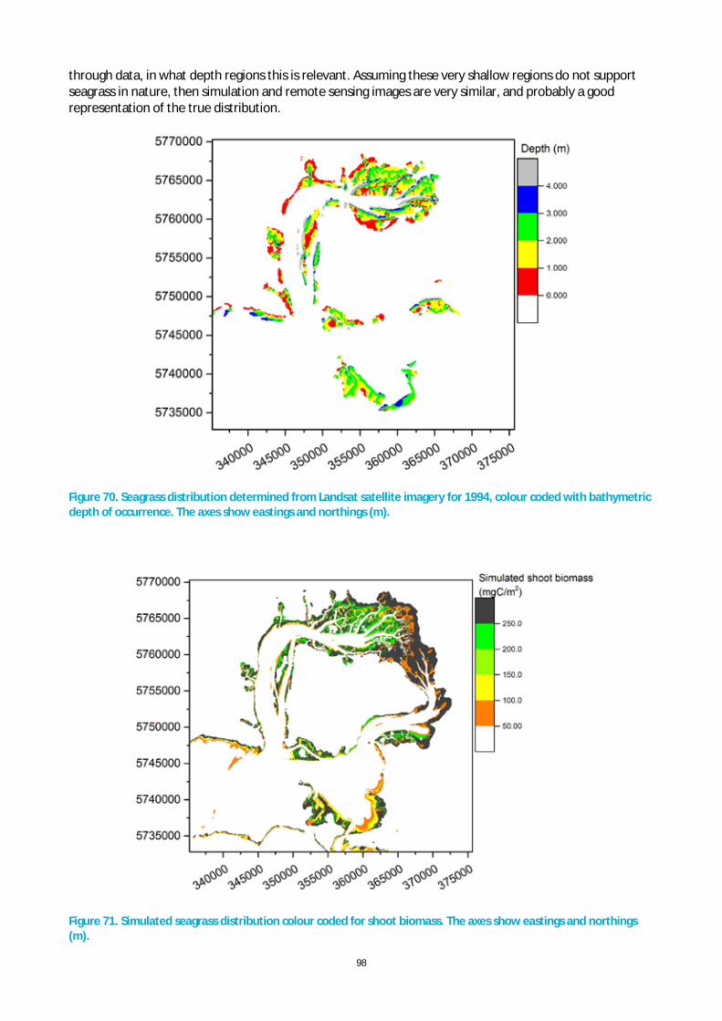
98

through data, in what depth regions this is relevant. Assuming these very shallow regions do not support seagrass in nature, then simulation and remote sensing images are very similar, and probably a good representation of the true distribution.

Figure 70. Seagrass distribution determined from Landsat satellite imagery for 1994, colour coded with bathymetric depth of occurrence. The axes show eastings and northings (m).

Figure 71. Simulated seagrass distribution colour coded for shoot biomass. The axes show eastings and northings (m).

99

Figure 72. Simulated seagrass distribution colour coded for shoot density. The axes show eastings and northings (m).

6.5 Conclusions

6.5.1 FINDINGS

The model has illustrated the effect of linkages between seagrass, light availability and sediment transport in Western Port. Seagrass extent is strongly controlled by light availability in Western Port. Both water quality and water depth impact on light availability. One metre of sealevel rise would be sufficient to substantially reduce seagrass extent within its existing range. Increase in water temperature would also reduce seagrass extent. The relative sensitivities can be explored.

6.5.2 LIMITATIONS AND RECOMMENDATIONS

There is space for further extension of the seagrass model. The calculation of seagrass density dependent shear stress can be calculated using a modified wave friction factor (Newell and Koch 2004) passed back to the ELCOM model in each computational time step. An epiphyte submodel could be modelled according to the formulation of Plus et al. (2003). An obvious addition would be a more in-depth implementation of internal nutrient pools, e.g. using also phosphorous and/or splitting nutrient pools into above and below ground pools (see e.g., Plus et al. 2003). However, for this project we would like to keep the model as simple as possible while having a good as possible representation of the major processes implemented specific for Western Port. None of the above listed models has the capacity to simulate the spread of seeds or tubers to handle colonization of neighbouring cells (e.g., Ruiz Montoya et al 2012, Meire et al 2014). A future extension could be the inclusion of such dispersal via, e.g., a cellular automata approach. Only by using such a dispersal functionality one can run multi-year scenarios describing recolonising of previously lost seagrass beds. The simulation tool discussed above will only be able to see if the current physical state is suitable for growth or if it is prone to decline. Whenever a cell has lost its seagrass population in the model, there is no way to handle recolonization.

100

During the course of model development several gaps or model limitations came apparent. To close these gaps and improve simulation results we recommend the following actions:

Model and process specific actions

· gather more data and physiologic parameters for model parameterization, · research parameterization of missing processes, e.g. tidal flats without seagrass need to be an

output of the model, epiphyte coverage of seagrass and growth in the bay, · implement heat balance model for simulation of water temperature from meteorological data to

substitute empirical relation,

Data specific actions

· implement a higher resolved bathymetry, · monitoring of seagrass density at specific locations over several seasonal cycles (model can be used

to hint for locations), · monitoring of in situ underwater light climate over time and space, · collect and homogenize available meteorological data in the region to generate a viable time series

over the last century, · reconstruct historical sealevels over several decades.

Next steps in combining remote sensing and seagrass modelling

· assimilation of remote sensing data for light adsorption (kd) into the seagrass model, · transfer seagrass implementation to parallel computation to significantly speed up run times

(expect a factor of up to 1/100), · user friendly interface to allow for out-of-house application, · testing the effect of river loading during high flow events by following (remote sensing) and/or

simulating (ELCOM) plume development and its effect on light climate and seagrass, · implement seagrass model into ELCOM/CAEDYM to combine with sediment resuspension

processes,

These steps would allow for short- as well as long-term scenario modelling of seagrass distribution based on characteristic river loading to the bay and connect them to remote sensing data as well as field monitoring.

101

References

Abal EG, Dennison WC. 1996. Seagrass depth range and water quality in southern Moreton bay, Queensland, Australia. Marine and Freshwater Research, 47: 763-771. 10.1071/mf9960763.

Abdelrhman MA. 2003. Effect of eelgrass Zostera marina canopies on flow and transport. Mar Ecol Prog Ser, 248; 67–83. doi:10.3354/meps248067.

Abernethy B, Rutherfurd ID. 2001. The distribution and strength of riparian tree roots in relation to riverbank reinforcement. Hydrological processes, 15: 63-79, doi: 10.1002/hyp.1152.

Adi NS, Phinn S, Roelfsema C. 2013. Estimating the diffuse attenuation coefficient from moderate spatial resolution, multi-spectral satellite data in a seagrass environment, 2013 IEEE International Geoscience and Remote Sensing Symposium - IGARSS, Melbourne, VIC, 2013, 310-313. doi: 10.1109 /IGARSS.2013.6721154

Ahnert K, Mulansky M. 2011. Odeint - Solving ordinary differential equations in C++. arXiv:1110.3397 [cs.MS], doi:10.1063/1.3637934.

Armanini A. 1992. Variations of bed and sediment load mean diameters due to erosion and deposition processes, Dynamics of Gravel Bed Rivers, Edited by P Billi, RG Hey, CR Thorne and P Tacconi, 351-359.

Aveytua-Alcazar L, Camacho-Ibar VF, Souza, AJ, Allen JI, Torres R. 2008. Modelling Zostera marina and Ulva spp. in a coastal lagoon. Ecol Model, 218 (3-4): 354–366. doi:10.1016/j.ecolmodel.2008.07.019.

Bach HK, 1993. A dynamic model describing the seasonal variations in growth and the distribution of eelgrass (Zostera Marina L) - 1. Model theory. Ecol Model 65 (1-2): 31–50. doi:10.1016/0304-3800(93)90125-c.

Baird ME, Adams MP, Babcock RC, Oubelkheir K, Mongin M, Wild-Allen KA, Skerratt J, Robson BJ, Petrou K, Ralph PJ, O’Brien KR, Carter AB, Jarvis JC, Rasheed MA. 2016. A biophysical representation of seagrass growth for application in a complex shallow-water biogeochemical model. Ecol Mod, 325: 13-27. doi:10.1016/j.ecolmodel.2015.12.011.

Blake S, Ball D. 2001. Victorian Marine Habitat Database: Seagrass Mapping of Western Port. Geospatial Systems Section, Marine and Freshwater Resources Institute Report No. 29.

Bocci M, Coffaro G, Bendoricchio G. 1997. Modelling biomass and nutrient dynamics in eelgrass (Zostera marina L.): Applications to the Lagoon of Venice (italy) and Øresund (Denmark). Ecological Modelling, 102 (1): 67–80.

Booij N, Ris RC, Holthuijsen LH. 1999. A third-generation wave model for coastal regions - 1. Model description and validation. Journal of Geophysical Research C, 104: 7649-7666. 10.1029/98jc02622.

Bos AR, Bouma TJ, de Kort GLJ, van Katwijk MM. 2007. Ecosystem engineering by annual intertidal seagrass beds. Sediment accretion and modification. Estuarine and Coastal Shelf, S74: 344–348. 10.1016/j.ecss.2007.04.006.

Brando VE, Schroeder T, Dekker AG, Blondeau-Patissier D. 2008. MTSRF Project 3.7.9 –Remote Sensing of GBR wide water quality: RWQPP Marine Monitoring Program, Milestone Report for Reef Water Quality Protection Plan (RWQPP) Marine Monitoring Program, CSIRO Land and Water Report, 20 November 2008, Canberra.

Brando VE, Anstee JM, Wettle M, Dekker AG, Phinn SR, Roelfsema C. 2009. A physics based retrieval and quality assessment of bathymetry from suboptimal hyperspectral data. Remote Sensing of Environment, 113: 755-770. doi:10.1016/j.rse.2008.12.003.

Brizga S, Condina P, Craigie NM et al. 2001. Northern waterways of Western Port geomorphological and water quality management study (incorporating floodplain re-engagement feasibility assessment). Report RM2006/J5272. A report for Melbourne Water.

Bulthuis DA. 1977. Phytoplankton biomass and productivity in Western Port: preliminary data. Paper 179. Environmental Studies Series, Ministry for Conservation, Victoria.

Bulthuis DA. 1981. Distribution and Summer Standing Crop of Seagrass and Macro-algae in Western Port. Victoria. Proceedings of the Royal Society of Victoria, 92: 107-112.

102

Bulthuis DA. 1983a. Effects of insitu light reduction on density and growth of the seagrass heterozostera-tasmanica (martens ex aschers) den hartog in Western Port, Victoria, Australia. J Exp Mar Biol Ecol, 67 (1), 91–103. doi:10.1016/0022-0981(83)90137-5.

Bulthuis DA. 1983b. A Report of the Status of Seagrass in Western Port in May 1983. Internal Report Series, No. 38 Marine Science Laboratories.

Bulthuis DA. 1984. Loss of Seagrass in Western Port, a Proposal for Further Research, 1984/85. Marine Science Laboratories. Internal Report Series, No. 72. Ministry for Conservation. Victoria. Catchment Research pty ltd. 2012. Reparameterisation of the Port Phillip Bay and Western Port Catchment Model and Future Work to be Undertaken. Catchment Research Pty Ltd.

Bulthuis DA. 1987. Effects of temperature on photosynthesis and growth of seagrasses. Aquat Bot 27 (1), 27–40. doi:10.1016/0304-3770(87)90084-2.

Bulthuis DA, Axelrad DM, Mickelson MJ. 1992. Growth of the Seagrass Heterozostera-Tasmanica Limited by Nitrogen in Port Phillip Bay, Australia. Mar Ecol Prog Ser 89 (2-3), 269–275. doi:10.3354/meps089269.

Bulthuis DA, Brand GW. 1975. Seagrasses in relation to erosion and water quality in Western Port, Victoria. Australian Marine Science Bulletin 55: 6.

Bulthuis DA, Woelkerling WJ. 1983a. Seasonal Variation in Standing Crop, Density and Leaf Growth Rate of the Seagrass, Heterozostera tasmanica (Martens ex Aschers.) den Hartog in Western Port and Port Phillip Bay, Vic. Australia. Aquatic Botany, 16: 111-136.

Bulthuis DA, Woelkerling WJ. 1983b. Biomass accumulation and shading effects of epiphytes on leaves of the seagrass, Heterozostera-Tasmanica, in Victoria, Australia. Aquat Bot ,16 (2): 137–148. doi:10.1016/0304-3770(83)90089-x.

Burkholder JM, Tomasko DA, Touchette BW. 2007. Seagrasses and eutrophication. J Exp Mar Biol Ecol, 350 (1-2): 46–72. doi:10.1016/j.jembe.2007.06.024.

Campbell G, Phinn SR, Daniel P. 2011. The specific inherent optical properties of three sub-tropical and tropical water reservoirs in Queensland, Australia, Hydrobiologia, 658(1): 233-252.

Carr JA, D'Odorico P, McGlathery KJ, Wiberg PL. 2012a. Modeling the effects of climate change on eelgrass stability and resilience: future scenarios and leading indicators of collapse. Mar Ecol Prog Ser, 448: 289–301. doi:10.3354/meps09556.

Carr JA, D'Odorico P, McGlathery KJ, Wiberg PL. 2012b. Stability and resilience of seagrass meadows to seasonal and interannual dynamics and environmental stress. J Geophys Res-Biogeo 117. doi:10.1029/2011jg001744.

Cheng NS. 2013. Calculation of Drag Coefficient for Arrays of Emergent Circular Cylinders with Pseudofluid Model. J Hydraul Eng-Asce, 139 (6): 602–611. doi:10.1061/(Asce)Hy.1943-7900.0000722.

Church JA et al. 2013: Sea Level Change. In: Climate Change 2013: The Physical Science Basis. Contribution of Working Group I to the Fifth Assessment Report of the Intergovernmental Panel on Climate Change. Cambridge University Press.

Collier CJ, Waycott M, McKenzie LJ. 2012. Light thresholds derived from seagrass loss in the coastal zone of the northern Great Barrier Reef, Australia. Ecological Indicators, 23: 211-219. 10.1016/j.ecolind.2012.04.005.

Dale BH, Pooley GJ. 1979. Westernport input streams assessment Preliminary report to May 1976. Publication No. 232. Westernport regional environmental study. Ministry for Conservation, Victoria.

Darnell R, Henderson B, Kroon FJ, Kuhnert P. 2012. Statistical power of detecting trends in total suspended sediment loads to the Great Barrier Reef. Marine Pollution Bulletin, 65: 203-209. doi:10.1016/j.marpolbul.2012.04.002.

de Boer W F. 2007. Seagrass-sediment interactions, positive feedbacks and critical thresholds for occurrence: a review. Hydrobiologia, 591: 5–24. doi:10.1007/s10750-007-0780-9.

Dekker AG, Phinn SR, Anstee J, Bissett P, Brando VE, Casey B, Fearns P, Hedley J, Klonowski W, Lee ZP, Lynch M, Lyons M, Mobley CD, Roelfsema C. 2011. Intercomparison of shallow water bathymetry, hydro-optics, and benthos mapping techniques in Australian and Caribbean coastal environments. Limnology and Oceanography: Methods, 9: 396-425. 10:4319/lom.2011.9.396.

del Barrio P, Ganju NK, Aretxabaleta AL, Hayn M, García A, Howarth RW. 2014. Modeling future scenarios of light attenuation and potential seagrass success in a eutrophic estuary. Estuarine, Coastal and Shelf Science, 149: 13–23. doi:10.1016/j.ecss.2014.07.005.

103

Environmental Protection Authority. 1996. The Western Port Marine Environment. EPA Publication 493. Fabricius KE, Logan M, Weeks S, Brodie J. 2014. The effects of river run-off on water clarity across the central

Great Barrier Reef. Marine pollution bulletin, 84: 191-200. doi:10.1016/j.marpolbul.2014.05.012. French T, Monk J, Ierodiaconou D, Pope A, Ball D. 2014. Yaringa and French Island Marine National Park

Habitat Mapping. Parks Victoria Technical Series No. 96. Parks Victoria, Melbourne Gippel CJ. 1995. Potential of turbidity monitoring for measuring the transport of suspended solids in streams.

Hydrological Processes, 9: 83-97, doi:10.1002/hyp.3360090108. Graf WL. 1977. Rate law in fluvial geomorphology. American Journal Of Science, 277: 178-191. Hancock GJ, Olley JM, Wallbrink PJ. 2001. Sediment transport and accumulation in Western Port. Technical

Report 47/01. CSIRO Land and Water. Hardie R, Ivezich M, Phillipson S. 2012. Can riparian revegetation limit the scale and extent of flood related

stream erosion in Victoria, Australia? In: 6th Australian Stream Management Conference, Grove J, Rutherfurd ID (eds.), pp: 190-196.

Harris JE, Hinwood JB, Marsden MAH, Sternberg RW. 1979. Water movements, sediment transport and deposition, Western-Port, Victoria. Mar. Geol., 30: 131-161. 10.1016/0025-3227(79)90010-0.

Hawdon A, Keen R, Vleeshouwer J. 2009. Remote Automated Water Quality Stream Gauging System Design. In: Science Report 24/09, CSIRO Land and Water.

Herb WR, Stefan HG. 2005. Dynamics of vertical mixing in a shallow lake with submersed macrophytes. Water Resour Res 41 (2). doi:10.1029/2003wr002613.

Herzfeld M, Waring JR. 2008. SHOC: Sparse Hydrodynamic Ocean Code User’s manual. CSIRO internal document. p 128.

Herzfeld M, Waring RJ, Parslow J, Margvelashvili N, Sakov P, Andrewartha J. 2008. SHOC: Sparse Hydrodynamic Ocean Code Science manual. CSIRO internal document. 121 pp.

Hipsey M, Antenucci JP, Hamilton DP. 2015. Computational Aquatic Ecosystem Dynamics Model: CAEDYM v3: v3.2 Science Manual. University of Western Australia.

Holland D, Cook P, Mac Nally R, Thomson J, Womersley B, Ball D, Longmore A, Keough M, Lee R, Martinez G, Greer D. 2013. Preliminary assessment of water quality requirements of seagrasses in Western Port, A report prepared for Melbourne Water, Water Centre Studies, Victoria.

Hughes AO, Prosser IP, Wallbrink PJ, Stevenson J. 2003. Suspended sediment and bedload budgets for the Western Port Bay basin. CSIRO Land and Water Technical Report 4/03, p 38.

Hurst TA. 2012. The Lang Lang Coast. A preliminary investigation of coastal erosion rates. Melbourne Water. Irish RR, Barker JL, Goward SN, Arvidson T. 2006. Characterization of the Landsat-7 ETM+ automated cloud-

cover assessment (ACCA) algorithm. Photogrammetric Engineering and Remote Sensing, 72: 1179-1188

Janse JH, Van Liere L. 1995. Pclake: A modelling tool for the evaluation of lake restoration scenarios. Water Science and Technology, 31 (8): 371–374. doi:10.1016/0273-1223(95)00392-Z.

Janse JH. 2005. Model Studies on the Eutrophication of Shallow Lakes and Ditches. Wageningen University. Janssen ABG, Teurlincx S, An S, Janse JH, Paerl HW, Mooij WM. 2014. Alternative stable states in large shallow

lakes. Journal of Great Lakes Research. 10.1016/j.jglr.2014.09.019. Jöhnk KD. 2005. Heat Balance of Open Water Bodies. In: Lehr, J.H. & Keeley, J. (eds.) Water Encyclopedia,

Vol. 3: Surface and Agricultural Water, John Wiley & Sons Publ., 190-193. doi: 10.1002/047147844X.sw398

Kenov IA, Deus R, Alves CN, Neves R. 2013. Modelling Seagrass Biomass and Relative Nutrient Content. J Coastal Res, 29 (6): 1470–1476. doi:10.2112/jcoastres-d-13-00047.1.

King P, Kay D. 1980. Westernport Regional Environmental Study: land use and erosion control guidelines for the Western Port catchment. Ministry for Conservation, Victoria Environmental Program.

Kirk JTO. 1984. Dependence of relationship between inherent and apparent optical properties of water on solar altitude. Limnology and Oceanography, 29: 350–356.

Koch EW, Beer S. 1996. Tides, light and the distribution of Zostera marina in Long Island Sound, USA. Aquat Bot, 53 (1-2): 97–107. doi:10.1016/0304-3770(95)01015-7.

Kombiadou K, Ganthy F, Verney R, Plus M, Sottolichio A. 2014. Modelling the effects of Zostera noltei meadows on sediment dynamics: application to the Arcachon lagoon. Ocean Dynam, 64 (10): 1499–1516. doi:10.1007/s10236-014-0754-1.

104

Kroon FJ, Kuhnert PM, Henderson BL, Wilkinson SN, Kinsey-Henderson A, Abbott B, Brodie JE, Turner DR. 2012. River loads of suspended solids, nitrogen, phosphorus and herbicides to the Great Barrier Reef lagoon. Marine Pollution Bulletin, 65: 167–181. http://dx.doi.org/10.1016/j.marpolbul.2011.10.018.

Lee Z, Carder KL, Mobley CD, Steward RG, Patch JF. 1999. Hyperspectral remote sensing for shallow waters: II. deriving bottom depths and water properties by optimization. Applied Optics, 38: 3831-3843.

Lee ZP, Carder KL, Steward RG, Peacock TG, Davis CO, Patch JS. 1998. An empirical algorithm for light absorption by ocean water. Journal of Geophysical Research, 103: 27,967-927,978.

Lee Z, Kendall LC, Chen RF, Peacock TG. 2001. Properties of the water column and bottom derived from Airborne Visible Imaging Spectrometer (AVIRIS) data. Journal of Geophysical Research, 106: 11,639-611,651.

Lee KS, Park SR, Kim YK. 2007. Effects of irradiance, temperature, and nutrients on growth dynamics of seagrasses: A review. J Exp Mar Biol Ecol, 350 (1-2): 144–175. doi:10.1016/j.jembe.2007.06.016.

Leoni V, Vela A, Pasqualini V, Pergent-Martini C, Pergent G. 2008. Effects of experimental reduction of light and nutrient enrichments (N and P) on seagrasses: a review. Aquatic Conservation-Marine and Freshwater Ecosystems, 18 (2): 202–220. doi:10.1002/aqc.842.

Li F, Jupp DL, Reddy S, Lymburner L, Mueller N, Tan P, Islam A. 2010. An evaluation of the use of atmospheric and BRDF correction to standardize Landsat data. IEEE Journal of Selected Topics in Applied Earth Observations and Remote Sensing, 3: 257-270.

Lowe M. 1999. Sediment sources in Western Port catchment. In: Unpublished thesis, University of Melbourne.

Marsden MAH, Mallett CW, Donaldson AK. 1979. Geological and physical setting, sediments and environments, Western-Port, Victoria. Mar. Geol., 30: 11-46. doi:10.1016/0025-3227(79)90004-5.

Masek JG, Vermote EF, Saleous N, Wolfe R, Hall FG, Huemmrich F, Gao F, Kutler J, Lim TK. 2006. A Landsat surface reflectance data set for North America, 1990-2000, Geoscience and Remote Sensing Letters, 3: 68-72.

McInnes KL, Macadam I, O'Grady J. 2009. Effect of climate change on extreme sea levels along Victorias Coast. CSIRO Climate Adaptation Flagship, p 55.

Meals DW, Dressing SA, Davenport TE. 2010. Lag Time in Water Quality Response to Best Management Practices: A Review. Journal of Environmental Quality, 39: 85-96. doi:10.2134/jeq2009.0108.

Meire DWSA, Kondziolka JM, Nepf HM. 2014. Interaction between neighboring vegetation patches: Impact on flow and deposition. Water Resour Res, 50 (5): 3809–3825. doi:10.1002/2013wr015070.

Melbourne Water, 2011. Understanding the Western Port Environment. Melbourne Water, p 228. Morris L, Jenkins G, Hatton D, Smith T. 2007. Effects of nutrient additions on intertidal seagrass (Zostera

muelleri) habitat in Western Port, Victoria, Australia. Mar. Fresh. Res. 58 (7): 666–674. doi:10.1071/mf06095.

Newell RIE, Koch EW. 2004. Modeling seagrass density and distribution in response to changes in turbidity stemming from bivalve filtration and seagrass sediment stabilization. Estuaries 27 (5): 793–806. doi:10.1007/bf02912041.

Norris R, Dyer F, Hairsine P, Kennard M, Linke S, Merrin L, Read A, Robinson W, Ryan C, Wilkinson S, Williams D. 2007. Australian Water Resources 2005, Assessment of river and wetland health: Testing the framework. National Water Commission.

Pedersen TM, Gallegos CL, Nielsen SL. 2012. Influence of near-bottom re-suspended sediment on benthic light availability. Estuar Coast Shelf S 106, 93–101. doi:10.1016/j.ecss.2012.04.027.

Pierson DC, Kratzer S, Strömbeck N, Håkansson B. 2008. Relationship between the attenuation of downwelling irradiance at 490 nm with the attenuation of PAR (400 nm–700 nm) in the Baltic Sea, Remote Sensing of Environment, 112(3): 668-680.

Plus M, Chapelle A, Menesguen A, Deslous-Paoli JM, Auby I. 2003. Modelling seasonal dynamics of biomasses and nitrogen contents in a seagrass meadow (Zostera noltii Hornem.): application to the Thau lagoon (French Mediterranean coast). Ecol Model 161 (3): 213–238.

Purss MB, Lewis A, Oliver S, Ip A, Sixsmith J, Evans B, Edber, R, Frankish G, Hurst L, Chan T. 2015. Unlocking the Australian Landsat Archive–From dark data to High Performance Data infrastructures, GeoResJ, 6: 135-140.

Roberts D. 1985. From swampland to farmland: a history of the Koo-Wee-Rup Flood Protection District. Rural Water Commission of Victoria.

105

Rogers K, Saintilan N, Heijnis H. 2005. Mangrove encroachment of salt marsh in Western Port Bay, Victoria: the role of sedimentation, subsidence and sea level rise. Estuaries, 28: 551-559.

Rutherfurd ID. 2000. Some human impacts on Australian stream channel morphology. In: River Management: The Australasian Experience. Brizga S, Finlayson B (eds.) John Wiley and sons, 11-49.

Ruiz-Montoya L, Lowe RJ, van Niel KP, Kendrick GA. 2012. The role of hydrodynamics on seed dispersal in seagrasses. Limnol. Oceangr. 57 (5), 1257–1265. doi:10.4319 /lo.2012.57.5.1257.

Sachse R, Petzoldt T, Blumstock M, Moreira S, Pätzig M, Rücker J, Janse JH, Mooij WM, Hilt S. 2014. Extending one-dimensional models for deep lakes to simulate the impact of submerged macrophytes on water quality. Environmental Modelling & Software, 61: 410–423. doi:10.1016/j.envsoft.2014.05.023.

Salo T, Pedersen MF. 2014. Synergistic effects of altered salinity and temperature on estuarine eelgrass (Zostera marina) seedlings and clonal shoots. J Exp Mar Biol Ecol, 457, 143–150. doi:10.1016/j.jembe.2014.04.008.

Sand-Jensen K. 1977. Effect of epiphytes on eelgrass photosynthesis. Aquatic Botany, 3: 55–63. doi:10.1016/0304-3770(77)90004-3.

Sand-Jensen K. 2003. Drag and reconfiguration of freshwater macrophytes. Freshwater Biol 48 (2), 271–283. doi:10.1046/j.1365-2427.2003.00998.x.

Sargeant I. 1977. A review of the extent and environmental effects of erosion in the Westernport catchment. Westernport regional environmental study. Environmental Studies Series publication no. 174. Ministry for conservation, Victoria.

Shepherd SA, Watson JE, Womersley HBS, Carey JM. 2009. Long-term changes in macroalgal assemblages after increased sedimentation and turbidity in Western Port, Victoria, Australia. Botanica Marina, 52: 195-206. doi:10.1515/bot.2009.036.

Short FT, Neckles HA. 1999. The effects of global climate change on seagrasses. Aquat Bot, 63: (3-4), 169–196. doi:10.1016/s0304-3770(98)00117-x.

Stephens AC. 1995. Seagrass in Western Port, Victoria. Australia. Environment Protection Authority, No. 490. Victoria. Australia.

Stewart J. 2012. Reparameterisation of the Port Phillip Bay and Western Port Catchment Model. Report Prepared for the Victorian EPA and Melbourne Water, p 30.

Tilstone GH, Peters SW, van der Woerd HJ, Eleveld MA, Ruddick K, Schönfeld W, Krasemann H, Martinez-Vicente V, Blondeau-Patissier D, Röttgers R, Sørensen K, Jørgensen PV, Shutler JD. 2012 Variability in specific-absorption properties and their use in a semi-analytical ocean colour algorithm for MERIS in North Sea and Western English Channel Coastal Waters. Remote Sensing of Environment, 118: 320-338 doi:10.1016 /j.rse.2011.11.019.

Toffaleti FB. 1968. Technical report No. 5. A procedure for computation of total river sand discharge and detailed distribution, bed to surface, Committee on Channel Stabilization, U.S. Army Corps of Engineers.

Tomkins K, McLachlan G, Coleman R. 2014. Quantification of coastal bank erosion rates in Western Port. CSIRO Water for a Healthy Country, p 70.

Vaudrey JMP, Kremer JN, Branco BF, Short FT. 2010. Eelgrass recovery after nutrient enrichment reversal. Aquat Bot, 93 (4): 237–243. doi:10.1016/j.aquabot.2010.08.005.

Verhagen J, Nienhuis PH. 1983. A simulation model of production, seasonal changes in biomass and distribution of eelgrass (Zostera marina) in Lake Grevelingen. Marine Ecology-Progress Series, 10: 187–195.

Wallbrink PJ, Hancock GJ, Olley JM, Hughes A, Prosser IP, Hunt D, Rooney G, Coleman R, Stevenson J. 2003a. The Westernport sediment study. Consultancy Report, CSIRO Land and Water.

Wallbrink PJ, Olley JM, Hancock G. 2003b. Tracer assessment of catchment sediment contributions to Western Port, Victoria. Technical Report 8/03. CSIRO Land and Water, Canberra

Waters D, Packett R. 2007. Sediment and nutrient generation rates for Queensland rural catchments – an event monitoring program to improve water quality modelling. In: Proceedings of the 5th Australian Stream Management Conference, Charles Sturt University, p 425-430.

Wettle M, Brando VE. 2006. SAMBUCA - Semi-analytical model for Bathymetry, un-mixing and concentration assessment. CSIRO Land and Water Science Report No. 22/06. CSIRO, Canberra.

106

Wilk RR, Keene JB, Marden MAH. 1979. Sediment characteristics in the embayment head of Western Port - The impact of swamp drainage and erosion on sedimentation and seagrass distribution. Environmental Studies Series Publication No. 24. Ministry of Conservation, Victoria.

Wilkinson S, Henderson A, Chen Y, Sherman B. 2004. SedNet User Guide, Version 2. CSIRO Land and Water. Wilkinson SN. 2012. Mean-annual sediment loads and ambient concentrations: Two sides of the same coin

or different kettles of fish? In: 6th Australian Stream Management Conference, Grove J, Rutherfurd ID (eds.).

Wilson P. 2014. Collecting 29,000 km of river condition data using LiDAR and aerial photography In: 7th Australian Stream Management Conference. Vietz G, Rutherfurd ID, Hughes R (Eds.), 427-435.

White NJ, Haigh ID, Church JA, Koen T, Watson CS, Pritchard TR, Watson PJ, Burgette RJ, McInnes KL, You ZJ, Zhang X, Tregoning P. 2014. Australian sea levels—Trends, regional variability and influencing factors. Earth-Science Reviews, 136: 155–174. doi:10.1016/j.earscirev.2014.05.011.

Zharova N, Sfriso A, Voinov A, Pavoni B. 2001. A simulation model for the annual fluctuation of Zostera marina biomass in the Venice lagoon. Aquat Bot, 70 (2): 135–150. doi:10.1016/s0304-3770(01)00151-6.

107

108

CONTACT US t 1300 363 400 +61 3 9545 2176 e enquiries@csiro.au w www.csiro.au

YOUR CSIRO Australia is founding its future on science and innovation. Its national science agency, CSIRO, is a powerhouse of ideas, technologies and skills for building prosperity, growth, health and sustainability. It serves governments, industries, business and communities across the nation.

FOR FURTHER INFORMATION CSIRO Land and Water Scott Wilkinson t +61 2 6246 5582 e scott.wilkinson@csiro.au w www.csiro.au/Land-and-Water w http://people.csiro.au/W/S/Scott-Wilkinson CSIRO Land and Water Klaus Joehnk t +61 2 6246 5636 e Klaus.Joehnk@csiro.au w http://www.csiro.au/Land-and-Water w http://people.csiro.au/J/K/Klaus-Joehnk