Welfare Rules, Incentives, and Family Structure*

Robert A. Moffitt Johns Hopkins University

Brian J. Phelan DePaul University

Anne E. Winkler University of Missouri-St. Louis

First Draft: June 2015 Current Draft: February 2018

Abstract

We provide a new examination of the incentive effects of welfare rules on family structure among low-income women by emphasizing that the eligibility and benefit rules in the AFDC and TANF programs are based more on the biological relationship between the children and any male in the household than on marriage or cohabitation per se. Using data from 1996 through 2008, we analyze the effects of 1990s welfare reforms on family structure categories that incorporate the biological status of the male. Like past work, we find that most policies did not affect family structure. However, we do find that several work-related reforms increased single parenthood and decreased marriage to biological fathers. These results are especially evident when multiple work-related policies were implemented together and when we examine the longer term impacts of the policies. We posit that these effects of work-related welfare policies on family structure stem from their effects on increased labor force participation and earnings of single mothers combined with factors special to biological fathers, including a decline in their employment and wages.

JEL Codes: J12, J18, I38 Keywords: Welfare Reform, Family Structure

* The authors would like to thank the National Institutes of Health under R01 HD 27248 and the Hopkins PopulationCenter under R24 HD042854 for partial support of this project. We also thank Thomas DeLeire, two anonymous referees, Marianne Bitler, Lynn Cook, Hilary Hoynes, Lenna Nepomnyaschy, Peter Orazem, and Chris Wimer as well as seminar participants at the University of Washington, Washington University in St. Louis, Duke University, the University of Wisconsin at Milwaukee, IZA, the SOLE sessions at the MEA Annual Conference, and the annual meetings of the Population Association of America and of the Association of Public Policy Analysis and Management for helpful feedback. Any remaining errors are our own.

1

A question of long-standing research and policy interest is whether the U.S. welfare

system discourages marriage and encourages single motherhood. The origin of this hypothesis

lies in the structure of the main welfare program through the early 1990s, the Aid to Families

with Dependent Children (AFDC) program, which was largely offered only to single parent

families. A large volume of research was conducted from the 1990s through the early 2000s on

whether AFDC affected family structure (Blackburn, 2003; Blau et al., 2004; Duncan and

Hoffman, 1990; Ellwood and Jencks, 2001; Hoffman and Foster, 2000; Lichter et al., 1991;

McLaughlin and Lichter, 1997; Moffitt et al., 1998; Winkler, 1995). Summaries of that research

(e.g., Moffitt, 1998) showed quite weak evidence for the hypothesis, albeit with a wide range of

estimates across different studies consistent with the existence of a nonzero positive effect on

single motherhood but one which is probably small in magnitude and hard to detect.

The more recent literature on this topic has concerned itself instead with the effect of a

major federal reform of the AFDC program in 1996 that imposed work requirements, time limits,

and other features on the program and renamed it the Temporary Assistance for Needy Families

(TANF) program. While most of the major features of the reform did not directly affect

incentives for different family structures, one clearly articulated goal of the legislation was to

reduce single motherhood.1 A body of research has examined whether this reform affected

different dimensions of family structure (Acs and Nelson, 2004; Bitler et al., 2004b; Bitler et al.,

2006; Blau and van der Klaauw, 2013; Dunifon et al., 2009; Ellwood, 2000; Fitzgerald and

Ribar, 2004; and Fraker et al., 2002), with an important new dimension in some of these studies

being whether cohabitation was affected by the law. Surveys of this broad literature (Blank,

1 These reforms were part of the Personal Responsibility and Work Opportunity Act (PRWORA) of 1996. The first section of the legislation is entirely devoted to documenting the rise in nonmarital births and it ends with the statement that “...it is the sense of Congress that prevention of out-of-wedlock pregnancy and reduction of out-of-wedlock births are very important government interests and [this legislation] is intended to address the crisis.”

2

2002; Grogger and Karoly, 2005; Lopoo and Raissian, 2014; Moffitt, 2007) have generally

summarized results on family structure as showing mixed effects, with a few studies finding

some significant effects but most finding no significant effects or a set of mixed effects with no

clear indications one way or the other.

Our study also analyzes the effects of welfare reform on family structure but advances the

literature by recognizing the importance of the biological relationship of any male in the

household to the children and explicitly introducing it into the empirical analysis. The AFDC

and TANF programs base eligibility not primarily on marital status but on the aforementioned

biological relationship. That is, the programs largely treat families the same, regardless of

whether the adults are married or cohabiting, if the male in the household is the biological father

of the children. If the male is not the biological father of the children, then the programs treat the

mother and her children completely differently.2 This distinction has been known for some time

(e.g. Winkler, 1995; Moffitt et al., 1994, 1998; Carlson et al., 2004), but most past work in this

area has instead considered the effects of welfare on a threefold classification of married,

cohabiting, or neither, regardless of the biological status of the male (two exceptions are

discussed later). This distinction is important in terms of magnitudes. For example, our data

show that 70% of low-income cohabiting mothers live with a male who is the biological father of

at least one of the mother’s children. Our study adds the biological relationship to the family

structure classification to determine whether the effects of the 1990s reforms had differential

effects depending on that relationship.

Our study also contributes to this literature by extending the empirical approach of Acs

and Nelson (2004) and Dunifon et al. (2009) to identify the effects of TANF reforms on family

2 We discuss the case of blended families – where some children are the biological children of the male and some are not – below.

3

structure. While the 1996 welfare reform law set federal standards for the new TANF program,

states were allowed to implement stricter versions of the various reforms (e.g., shorter time

limits) and were free to adopt or adjust other policies (e.g., two-parent eligibility policies, family

caps) if they so chose. Acs and Nelson (2004) and Dunifon et al. (2009) specified TANF policy

variables capturing this state-level policy variation and estimated the effects of those individual

policies on family structure.3 We construct an expanded set of individual TANF policy variables

and extend this approach further by also considering whether states adopted groups, or

“bundles,” of policies during the TANF period. Grouping policies into bundles helps address a

well-known problem in the study of these reforms, which is that often multiple reforms were

adopted simultaneously, making it difficult to identify their separate effects (Bitler et al., 2004b).

Therefore, the grouped policies may better identify the overall impact of the reform.

A final contribution of our study is that we examine the effects of 1990s welfare reform

over a longer period of time (from 1996 through 2008) than past studies, which have typically

not gone past 2000. Looking over a longer period of time will matter if family structure

decisions are slow to change in response to the changes in welfare rules.

For our analysis, we use data from the Survey of Income Program Participation (SIPP)

for the years 1996 (the interview took place just before implementation of the law), 2001, 2004,

and 2008. The SIPP is a particularly good data source for this analysis because it contains a

household relationship matrix identifying the biological relationships between the children and

all of the adults in the household. Thus, the SIPP is the only data source that allows us to both

create our family structure outcomes that incorporate detailed information on biological status

and which date back to the 1990s. In robustness tests, we also include the 1993 SIPP in our

3 Other papers in this literature (Bitler et al., 2004b, 2006; Blau and van der Klaauw, 2013) used variation in the date of implementation of TANF to identify the effects of TANF. However, the dates likely varied too little to have an effect on an outcome like family structure, which is likely to respond slowly.

4

analysis. Our primary sample excludes 1993, however, because an “unmarried partner” (i.e. a

cohabitor) was not identified as an explicit relationship alternative until the 1996 SIPP.

Like much of the past literature, we find that most welfare reform policies have not had a

significant effect on family structure. However, we do find that several work-related reforms,

implemented during both the waiver period and the TANF period, resulted in increases in single

motherhood and decreases in marriage to biological fathers. These effects are especially evident

when groups or bundles of work-related policies were implemented. These results are not at

odds with the literature, for some past studies have found that work-related reforms increased

single parenthood, decreased marriage, or both (Bitler et al., 2004b; Dunifon et al. 2009;

Ellwood, 2000; Fitzgerald and Ribar, 2004; Fraker et al., 2002; Gennetian and Knox, 2003).

Unlike our results, however, these past findings are sometimes of borderline significance or

nonrobust to specification. One important difference from these past studies is that we find that

the negative effects on marriage are limited to marriage to biological fathers (not stepfathers),

illustrating the importance of making biological distinctions. Additionally, we find that the

effects of work-related policies on family structure have grown over time, suggesting that the

long-run effects of welfare rules on family structure may be larger than the short-run effects.

We suggest several possible explanations for the decline in marriage to biological fathers

only, including one related to the decline in their employment and earnings. We also suggest

that the effects of work-related reforms on the increase in single motherhood may reflect the

importance of labor market outcomes on family structure. Work-related welfare reforms may

have increased female employment and earnings and made women more-able to support

themselves independently, leading to this increase in single parenthood (an interpretation also

given by Bitler et al., 2004b). This indirect effect of work-related welfare reforms on family

5

structure suggests that the recent policy proposals to impose work requirements on recipients of

the Supplemental Nutritional Assistance Program (SNAP) and the Medicaid program could

similarly increase the prevalence of single parent households (e.g., Goodnough, 2018).

In the following sections, we review AFDC welfare rules concerning family structure,

how they were altered by 1990s welfare reform, and discuss the expected effects of these rules

and reforms on family structure. Next, we discuss our approach and review the prior studies

which are closest to ours. We then present our data, methods, and results, followed by our

conclusions.

I. Welfare Rules and Their Family Structure Incentives

AFDC Family Structure Rules. The original 1935 Social Security Act which created the

AFDC program provided cash support to families with “dependent” children, who were defined

as those who were deprived of the support or care of one natural (i.e., biological) parent by

reason of death, disability, or absence from the home, and were under the care of the other parent

or a relative. Death was the primary reason for eligibility in 1935 but divorce and nonmarital

births rose as reasons for eligibility particularly after 1960. Thus, under the original rules, no

household with two biological parents was eligible for benefits, while the presence of a non-

biological adult in the household had no impact on the eligibility or benefits of an otherwise

eligible single-parent household. However, state agencies did not always enforce the law as it

was written and would often rule women as ineligible if there was any male in the household,

even temporarily. This practice was outlawed by a Supreme Court case in 1968 which

prohibited such “man-in-the-house” rules, reiterating that the presence of a male who was not

related to the children could not be used to determine eligibility.

6

A major change occurred in 1961, when Congress created the “Unemployed Parent”

program, which allowed states to make households with two biological parents eligible for

AFDC benefits if the principal earner had a significant work history but currently worked no

more than 100 hours per month. While this program (known as AFDC-UP) was initially

intended to provide supplementary benefits to families in cases of unemployment, it created a

way for two-parent households to be eligible for AFDC benefits. Indeed, when AFDC-UP was

expanded to include all states in 1988, one justification for its expansion was to promote

marriage.4 However, marital status was never a factor in determining eligibility for either the

AFDC “Basic” program (i.e., the program for single parent families) or the AFDC-UP program.

Congress also changed the way in which married non-biological adults (i.e. stepparents)

have been treated under AFDC. Traditionally, Congress left the decision on whether to include

or exclude stepparents from the assistance unit, and how to treat their income for purposes of

eligibility and benefit calculation, to the states. However, with the rise of stepparents starting in

the 1970s, Congress passed legislation in 1981 requiring that some portion of the income of

stepparents be “deemed” even if the step-parent is excluded from the assistance unit. This means

that some portion of the stepparent’s income must be counted in total income when assessing

eligibility and benefits received by the mother and her children.5 Nevertheless, states continue to

have the option of whether to include the stepparent in the assistance unit or not.

The incentive effects for family structure from these rules are clear. Cohabitation with or

marriage to a male who is not biologically related to the children is encouraged relative to

marriage or cohabitation with a biological father. This follows from the fact that a biological

4 Ultimately, AFDC-UP did not increase the number of two-parent families on the program by very much because of the stringent eligibility requirements (Winkler, 1995). 5 The 1981 rule is only relevant if the stepparent is excluded from the unit. If a stepparent is included in the unit, then all of the stepparent’s income is counted.

7

father’s income is always fully counted in the benefit and eligibility calculations, while the

income of an “unrelated” male (i.e., one not biologically related) is only partially

counted. Further, cohabitation with an unrelated cohabitor is generally encouraged relative to

marriage to an unrelated male (i.e., a stepparent) since some portion of the stepparent's income is

always counted against the benefit (although inclusion of the stepparent in the assistance unit

does raise the benefit level, which works the other way), whereas the income of unrelated

cohabitors is only counted against the benefit in certain states and in certain circumstances.6

This is one case where marital status does affect financial eligibility and benefit amounts – when

partners are unrelated to the children. As for incentives to marry rather than cohabit with a

biological father, these situations are treated identically by existing welfare rules.

Welfare Reform in the 1990s. The welfare rules changed dramatically with the 1996

welfare reform law (PRWORA), which replaced the existing program, AFDC, with TANF. The

major policy changes associated with the 1996 law, in addition to the fact that it converted the

AFDC funding mechanism from an entitlement to a block grant, are that it imposed a five-year

lifetime time limit on receipt of benefits; imposed work requirements with few exemptions and

with sanctions for noncompliance; imposed a separate time limit on the minimum amount of

time that could pass before work requirements were mandatory; offered states the option of

disregarding more earnings in benefit calculations (to provide work incentives); and offered

states the option of not increasing the family’s benefit if an additional child was born while on

welfare (the “family cap”). The legislation also abolished the AFDC-UP program and allowed

states to relax some or all of the restrictions governing eligibility of two-parent families (the 100-

6 The treatment of incomes of unrelated cohabitors in AFDC households varies widely across states, with some states counting cash contributions made for shared household expenses, some states considering whether the male pays for some portion of the rent, but others consider neither (Moffitt et al., 1994; Moffitt et al., 2009). We examine how changes in welfare rules from before 1996 to after 1996 affected family structure, and these rules did not change in a meaningful way over that period and hence are not studied here.

8

hour work rule, the work history requirement, etc.). Prior to 1996, states were allowed to test

similar reforms (time limits, work requirements, sanctions, earnings disregards, family caps, two-

parent rule modifications) by receiving a waiver from the federal government to do so. Thus,

some states had already moved partly toward the rules of TANF before 1996.

Our paper analyzes the effect of these reforms on family structure. Their expected effects

have been analyzed previously (Bitler et al., 2004b; Fitzgerald and Ribar, 2004; Grogger and

Karoly, 2005; Dunifon et al., 2009), though none discuss or recognize the biological distinctions

we make. A general conclusion from this past literature is that the expected effects of most

welfare reform policies on family structure are ambiguous. This conclusion persists even after

we refine the family structure variable to account for the biological relationship between the

mother’s children and any male living in the household. Specifically, we classify family

structure into five categories that arise naturally from the rule distinctions: whether a mother (1)

is a single parent (i.e. not in any union); (2) is married to the children’s biological father; (3) is

cohabiting with the children’s biological father; (4) is married to a man who is unrelated to the

children (stepfather); or (5) is cohabiting with an male unrelated to the children.

The reform policies can be divided into two types—family-oriented policies that are

intended to directly affect family structure, and work-related policies that are intended to affect

other outcomes (mainly employment and earnings) but which may have indirect effects on

family structure. The expected effects of both are summarized in Table 1. Family-oriented

policies include the relaxation of restrictive two-parent eligibility rules, the introduction of

family cap policies, and policies requiring the mandatory inclusion of a stepparent in the

assistance unit. The relaxation of two-parent eligibility rules should encourage the creation of

two biological parent households among welfare recipients, whether married or cohabiting,

9

because they make it easier for two-parent households to be eligible for welfare benefits. This

also means that they reduce the probability of being in other family structure types. However,

they may also simply move women who are already in biological unions onto the welfare rolls,

which implies no change in overall rates. Family cap policies, ignoring the effects on fertility

itself (discussed below), could affect family structure because they limit family benefits with the

birth an additional child, incentivizing the mother to seek additional income support. For

mothers who choose to remain on welfare, family caps incentivize partnering, either to a

biological father or an unrelated male, with the incentive much greater for the latter because the

man’s earnings are counted against the benefit to a lesser degree. The effective reduction in per-

person benefits associated with family caps might alternatively provide mothers on welfare with

an incentive to leave the program, which has, as we discuss below, ambiguous effects on family

structure. A mandate that stepparents be included in the assistance unit has an ambiguous effect

on the incentive to form stepparent families because the rule has an ambiguous effect on welfare

benefits.7 If the net effect is that potential benefits fall with the inclusion of the stepparent, then

step-parents will be discouraged relative to all other family types – especially unrelated

cohabitors. If potential benefits increase, the opposite would be true.

Work-related TANF policies—sanctions, work requirements, earnings disregards, and

time limits—could affect family structure indirectly, mainly through their effect on welfare

participation and labor force participation since each of these policies decreases the value of

being on welfare and discourages participation. Indeed, the most striking effect of the 1996

legislation was to dramatically reduce the caseload of the program (because of the sanctions,

work requirements, and time limits) and to increase the average level of work and earnings

7 On the one hand, it could decrease benefits since the inclusion of stepfathers in the assistance unit causes their earnings to be counted fully against the benefit. On the other hand, it could raise benefits because it increases the number of people in the assistance unit.

10

among low-income single mothers (Moffitt, 2003; Ziliak, 2016). However, welfare exit and

increased earnings have ambiguous effects on family structure. On the one hand, women who

leave the program will have an incentive to marry or cohabit, especially with biological fathers,

since there is no penalty for marrying or cohabiting when off welfare and they may seek out

male partners who have income to contribute to the household. On the other hand, one of the

oldest hypotheses in the economics literature on marriage is that the incentive to marry is

inversely related to the female wage rate and potential earnings, commonly called the

“independence effect” (Becker, 1991, p.336). Hence any work-encouraging welfare reform

component could decrease partnering (see Bitler et al., 2004b).8 It has also been noted that

TANF work requirements and sanctions are imposed on men included in the assistance unit

(Fraker et al., 2002). This creates an additional disincentive for women on welfare to marry or

cohabit with men while on welfare and could further cause work-oriented welfare reforms to

increase single motherhood.9

Lastly, our analysis follows the previous literature and ignores the fertility effects of these

rules by analyzing the effects of welfare rules on union formation conditional on the presence of

at least one child in the household. However, it is useful to briefly consider what types of effects

are possible. For example, family cap policies would be expected to reduce fertility since

benefits would not rise with additional children. Additionally, work-related policies may reduce

fertility, to the extent that fertility is negatively related to labor force participation. What is less

clear is how the potential reductions in fertility would be distributed across the family structure

8 The general equilibrium effect of increased female earnings could also make her a more attractive partner. This also makes the effect ambiguous in sign. 9 The social welfare implications of these expected effects are not clear. There is an argument to be made that program rules should be close to “family-structure” neutral, but it has been argued by others that the rules should promote marriage (for useful discussion, see Primus and Beeson, 2002). Moreover, the social welfare implications of family structure changes may differ depending upon whether the change is due to family related policies versus work-related reforms. These are interesting questions, but they are beyond the scope of our analysis.

11

alternatives and hence affect our results. In any case, the existing literature on 1990s welfare

reforms has found only mixed evidence that these reforms had any effect on fertility (Ziliak,

2016).

II. Contributions of This Study

Our main contribution, as already emphasized, is that we recognize the biological

distinction in welfare rules and incorporate the proper family structure outcomes into our

estimates of the effects of welfare reform on family structure. An additional contribution is that

we examine the effects of welfare rules over a longer period of time than any previous study,

which allows us to distinguish between short-run and long-run effects. However, in most other

respects, we follow the existing literature, combining the strengths of many previous studies.

For example, like Acs and Nelson (2004), we identify the effects of welfare reforms using a

difference-in-difference-in-differences strategy, comparing differences in trends in family

structure for a welfare-eligible group with a welfare-ineligible group across states that differ in

their welfare policies. We also follow the research design of Dunifon et al. (2009) by estimating

separate effects of pre-TANF waiver reforms and post-TANF variation in reforms. While many

studies have used state-level variation in waiver adoption to identify the effects of pre-TANF

waivers on family structure, only a few have used cross-state variation in post-TANF reform

elements. Then, we extend the Dunifon et al. (2009) approach by bundling the state-level TANF

policies using the approaches that Bitler et al. (2004b) and Ellwood (2000) applied to state-level

waiver policies.

Finally, we should note that two prior studies, Acs and Nelson (2004) and Blau and van

der Klaauw (2013), have incorporated biological relationships into family structure outcomes

12

when studying welfare reform. However, our study differs in important ways. Acs and Nelson

(2004) examined the effects of TANF welfare rules on the living arrangements of children,

defining those arrangements on the basis of the biological relationship of the adults to the

children. Our study design differs from theirs, however, because they only estimated the effect

of specific TANF components relative to the overall effect of TANF (they did not use waiver-

period variation, as we do); they only looked at three types of policies (sanctions, family caps,

and two-parent rules), whereas we look at seven; and their study only covered the years 1997 to

1999 for 13 states, whereas our study goes through 2008 and includes all 46 states in the SIPP

panels.10 Blau and van der Klaauw (2013) followed a cohort of women from 1979 through 2004

and estimated dynamic movements into and out of marriage and cohabitation and childbearing,

distinguishing between whether marriage and cohabitation occurred with the father of any

children born. Relative to our analysis, their measures of welfare reform are quite limited. They

included a single dummy for any pre-1996 waiver and a single dummy variable for TANF

implementation rather than the policy-element specification used in other analyses, including our

work. Additionally, by using only specific birth cohorts who were in their 30s by the time

welfare reform passed in 1996, they could not estimate its effects on younger age women who

constitute the majority of welfare recipients, nor could they separate age effects from period

effects.

III. Data and Methods

Data. For our empirical analysis, we use data on households from the SIPP. The SIPP is

a nationally representative household survey of the U.S. civilian noninstitutional population that

10 The 1996 and 2001 SIPP panels combined Maine and Vermont into one state and North Dakota, South Dakota, and Wyoming into another state. Thus, we exclude observations from these five states from all years of the analysis.

13

includes a series of panels starting in various years. Each panel follows households for

approximately four years and conducts core interviews and topical modules in each survey wave,

conducted approximately four months apart. The core questions in every wave of every panel

contain information on relationships between the reference person and other members of the

household, allowing us to identify spouses and cohabitors, where the latter is referred to as an

“unmarried partner.” The second wave of each panel further collects information from the

reference person regarding relationships between each member of the household and all other

members, including information on the biological relationships between each of the children and

the adults in the household. The core and the second-wave topical module questions are

combined to form what the SIPP calls the Household Relationship Matrix (HHRM). We use

these data to define our sample and to create variables that categorize family structure.11

Since the HHRM is only available in the second wave of each panel, we use data from

the second wave of the SIPP panels that began in 1993, 1996, 2001, 2004, and 2008.12 However,

our primary sample excludes data from the 1993 SIPP because the formal definition of a

cohabitor, an unmarried parent, was not included as a relationship type until the 1996 survey.

While the data for the second wave of the 1996 panel were collected between August and

November 2016 – largely after PRWORA was signed into law in August 1996 – it is highly

unlikely that family structure would change within three months in response to the law and, even

then, the states did not begin implementation until late 1996. Thus, we treat the 1996 data as our

“pre-law” period. However, we conduct a robustness test that includes data from 1993 SIPP and

11 The SIPP HHRM data are discussed in detail by Brandon (2007) and the Census Bureau issues periodic reports based on them. The first one, based on the 1996 panel, can be found in Fields (2001). 12 We cannot use the full SIPP panel because the HHRM is only available in the second wave. Thus, we cannot observe changes in all of our family structure variables across the other waves of each panel.

14

an alternative measure of cohabitation, to test the sensitivity of this assumption.13

For our sample, we select women 18-55 with a biological child age 17 or under living in

the household. Within this sample of mothers, we further distinguish between those mothers

who are more likely to be eligible for welfare and influenced by welfare policies (“Eligible”

sample) and those less likely to be eligible for welfare and influenced by welfare policies

(“Ineligible” sample). In the empirical analysis described below, we use this “Ineligible” sample

as an additional control group (in addition to the usual cross-state over-time variation) to

estimate the effects of welfare policies on family structure for the “Eligible” (i.e. targeted)

sample. We define Eligible as those who have less than 16 years of education and who have low

levels of assets since AFDC and TANF have asset tests. We define Ineligible as all other

mothers, either those with college degrees or non-college educated mothers with high assets.14

For the asset restriction, we exclude any family with cash in the bank greater than $3,000, that

owns any stocks or bonds or a retirement account, or that owns two or more cars. These cutoffs

are generally higher than the cutoffs for AFDC and TANF eligibility.15 As we show in Table 2,

welfare participation rates are much higher in the Eligible sample than in the Ineligible sample.

Thus, this restriction appears to achieve its goal, which is to create a comparison group of

Ineligible who almost never participate in welfare compared to an Eligible group who are much

more likely to participate and be influenced by welfare rules. The share of the sample that is 13 It is possible that states that did not enact waivers began to move toward the new welfare policies in informal ways that are not measured in the data, in anticipation of the 1996 legislation occurring. However, President Clinton’s signing of the legislation was a surprise, making this rather unlikely. In addition, to the extent such anticipatory actions took place in states without waivers, our estimates of welfare reform would be biased towards zero. 14 The labels “Eligible” and “Ineligible” are not meant to signify actual financial eligibility or ineligibility, and our “Eligible” group likely includes some families who are financially ineligible and our “Ineligible” group likely includes some families who are financially eligible. But, because education and assets are correlated with financial eligibility, the two groups have very different rates of participation in welfare, as we show below, and thus, are likely to be differentially affected by welfare rules. 15 Setting the asset restriction exactly equal to the eligibility cutoffs in the program would run the danger of possible endogeneity because it would exclude those individuals who could strategically reduce their assets to become eligible for the program and that is a participation choice.

15

Eligible and Ineligible also changes little over time, with the Eligible share ranging between 25.8

to 30.4 percent of the sample with no discernable trend. In the empirical work that follows, we

conduct sensitivity tests altering the asset restriction and the inclusion of college educated

mothers in the Ineligible sample.

For our main categorization of family structure, we identify male partners in the

household in two ways. First, we determine whether any male is classified as either a “spouse”

or an “unmarried partner”.16 For any male so identified, we use the HHRM to determine his

relationship to each of the children in the household. Second, we use the HHRM directly to

determine whether there is a male in the household with a common biological child with the

mother, even if not classified as a spouse or unmarried partner.17 Since our unit of observation is

a mother, we then separate women into those with a partner biologically related to some or all of

her children (“biological”), those with a partner biologically unrelated to all of her children

(“unrelated”), and those with no partner (“single parent”).18 Using this approach, we create our

five category family structure outcome, as described earlier and as shown in Table 2.

Table 2 shows the distribution of each family structure type in our sample, stratified by

eligibility type. For our sample of Eligible mothers, 45.1 percent had partners who were

biological fathers of the children, 6.3 percent had partners who were unrelated to the children,

and 48.6 percent had no partner and hence were single parents. Among those partnering with a

biological male, most were married but about 15 percent were cohabiting. Among those

16 As a practical matter, we do not have to use the core questions on relationships because the answers to those questions are incorporated into the HHRM; so the HHRM is the only data element we need for this purpose. 17 We excluded same-sex couples of which there were very few. 18 In cases in which the male has adopted the children, we define those families as biological families because that is how the AFDC and TANF programs treat them. In the case of blended families – those where the male or female is biological to some but not all of the children in the household – we group them with families where all children are biologically related to the male. We conduct a sensitivity test below that instead groups them with families where the male is unrelated to the children. It makes little difference to the results how they are classified because they constitute a small minority of households, just 4.4% to 5% for each of the four sample years.

16

partnering with an unrelated male, slightly more than half were married (i.e., stepparent families)

and the rest were cohabiting. Over the four years of data analyzed, 14 percent of Eligible

mothers participated in AFDC or TANF. The sample of Ineligible mothers were much more

likely to reside with a biological partner (78.5 percent) and much less likely to be a single parent

(15.1 percent). In addition, their welfare participation rate is only 1.3 percent, considerably

below the 14 percent for Eligible.19

Welfare Policy Variables. Our major independent variables of interest are those

measuring state-specific welfare reform elements, which we code separately for each of the four

years in our data. As noted in the last section, we follow the literature closely in the terms of the

policies examined and in how we define policies, although there are some slight differences

compared to past work. Similar to Bitler et al. (2004a) and Fitzgerald and Ribar (2004), we

group our policy variables into those that were intended to directly affect family structure

(“family-related” policies) and those that were intended to directly affect other outcomes but

may be indirectly related to family structure through their effect on welfare participation and

labor force participation (“work-related” policies). As shown in Table 3, we further separate the

work-related policies into waiver year (1996) variables and TANF year (2001, 2004, and 2008)

variables.

The work-related waiver variables capture variation in states’ adoption of sanctions, work

requirements, and expanded earnings disregard waivers. A sanction policy meant that families

who did not comply with one or more requirement, usually work requirements, would have their

benefits reduced in full or in part. A work requirement policy stipulated that mothers must begin

19 Like most reduced form analyses, our difference-in-difference methods compare family structure trends in these two groups and how they differentially respond to welfare reform. Because 1.3 percent of those in the Ineligible group participated in welfare (and were presumably influence by its rules), our coefficient estimates will be closer to zero than those that would be obtained if our comparison group had a zero welfare participation rate.

17

work within a specified time period and generally were required to work some minimum number

of hours per week. In general, an earnings disregard policy stipulates the amount of earnings that

can be deducted before counting income against the benefit. During welfare reform, many states

adopted waivers that made the earnings disregards more generous.

All the waiver variables in our analysis are lagged one year relative to the 1996 interview

date and coded as of December 1995 to avoid having to assume an instantaneous response of

family structure to changes in welfare rules.20 For sanctions and work requirement waivers, we

create dummy variables for a state’s having adopted such a policy. However, we code the

earnings disregard waiver equal to one if the state did not enact such a waiver so that its expected

effect on welfare participation (namely, negative) will be the same as that of the other two work-

related policies.

For TANF variables, one difference from many past studies is that we use state-level

variation in the implementation of specific TANF policies to help identify their effects on family

structure, rather than the timing of TANF implementation (Bitler et al., 2004b; Bitler et al., 2006;

Blau and Van der Klaauw, 2013; and Fitzgerald and Ribar, 2004). Thus, for our three TANF

years (2001, 2004, and 2008), we differentiate between states that adopted harsher versus less

severe policies, using variables similar to Acs and Nelson (2004) and Dunifon et al. (2009), both

of which implemented a similar empirical strategy. Like the waiver policies, we organize these

work-related TANF policies based on their expected effects on the welfare participation decision

because they should only affect family structure indirectly through that decision.

Specifically, we construct separate indicators for whether a state adopted the strictest

sanction policy, a time limit shorter than what was federally required, a more restrictive work

20 We do not include a time limit waiver variable because only two states had implemented this policy by December 1995.

18

exemption by age of the youngest child, and did not expand their earnings disregard. The

strictest sanction policy is defined as one that leads to the potential loss of the full family benefit

or the closure of the case. As for time limits, while the federal law mandated that no state could

use federal funds to pay a woman for more than five years of benefits, a number of states enacted

time limits shorter than that. Thus, we define a strict time limit as one shorter than five tears.

All states also had to specify the minimum age for the youngest child by which the mother was

required to work and the median age across all states was 12 months. We classify a state’s

policy as strict if it required mothers to work when their child reached an age younger than 12

months. Finally, the TANF law did not require any specific earnings disregard, so we code our

TANF earnings disregard variable identically to the waiver period variable.

We also include three family-related policies in our analysis. These variables reflect the

presence of a family cap on benefits, the (lack of) easing of the restrictive two-parent eligibility

rules, and the mandated inclusion of stepparents in the assistance unit. As we noted previously,

the sign and strength of the expected effects of these policies on family structure is ambiguous.

Thus, we code all three such that their effects tend to lower the rate of welfare participation, as

we code the work-related variables.

As discussed in Blank (2002), Grogger and Karoly (2005), and Moffitt and Ver Ploeg

(2001), and as we noted previously, the effects of each of the state policies may be difficult to

detect separately even if the overall effect of a group of policies is detectable. This is in part

because some individual reforms were not adopted by many states, different policies are often

correlated with one another, and the impact of multiple policies simultaneously may have been

larger than the sum of its parts. We address this concern by estimating the overall effect of a

group (or “bundle”) of reforms using variables for “any reform” and the “number of reforms.”

19

The “any reform” specification has been previously estimated in Bitler et al. (2004b), Bitler et al.

(2006), and Blau and van der Klaauw (2013); and the “number of reforms” specification has

been previously estimated in Ellwood (2000). However, different from past studies, we

construct these “bundle” measures separately for work-related policies in the waiver period,

work-related policies in the TANF period, and for family-related policies. Since we code the

individual policies in such a way that they have the same expected effects on welfare

participation, this gives the “any” and “number of” variables a coherent interpretation since the

indirect effects of these policies on family structure should come through the welfare

participation decision.21

As shown in Table 3, which briefly describes each of the individual and bundled welfare

policies used in our empirical analysis, these policies are well identified using state-year

variation. The one exception is our “Any Work-related Waiver” policy. We cannot construct an

“Any Work-related Waiver” policy using all three of our individual waiver policies because the

variable is not identified (i.e. it equals one for all states in 1996 and zero for all states in all other

years). To address this, we construct the “Any Work-related Waiver” variable using only two of

the policies (sanctions and work requirement), and include the third policy separately (no

expanded earnings disregard).

Other Policy and Control Variables. In our empirical analysis that follows, we control for

individual and household characteristics including the age, education, race and ethnicity of the

mother, and household urban residence. We also control for several other state-level transfer

programs and state-level labor market conditions which change differentially across states in an

21 The effects of each of the family-oriented policies are particularly difficult to predict and are ambiguous in sign (see Table 1) because they could have direct effects on family structure or indirect effects through effects on welfare participation, or both. Hence how to bundle them so that they have similar effects is inherently unclear. We tried some alternative bundling methods for these policies and found no change in the general pattern of estimated effects we present below (namely, usually insignificant and not robust).

20

effort to isolate the impact of changes in state-level welfare policies. These variables include:

the unemployment rate, the weekly manufacturing wage, the minimum wage, the maximum

welfare benefit, the Medicaid eligibility threshold (defined in terms of percentage above the

federal poverty line), and the maximum EITC benefit for a family of three (the Medicaid and

EITC variables include state supplements in addition to federally mandated levels). All such

variables are lagged one year and the dollar-denominated variables are measured in real terms.

The means of these variables for the Eligible and Ineligible samples are shown in Appendix

Table A1.22

Methods. We estimate models for alternative family structures with multinomial logit

(MNL) using our five-way family-structure classification as the outcome variable: households

with mothers who are married to the biological father of their children, who cohabit with a

biological father, who are married to an unrelated male (i.e., a stepfather), who cohabit with an

unrelated male, or who are single parents (i.e., no partner).

In estimating the MNL models we use a difference-in-difference-in-differences (DDD)

strategy, which compares differences in cross-state trends in family structure among Eligible

mothers with differences in cross-state trends in family structure among Ineligible mothers (as

defined earlier). This DDD approach, which has been used previously in this literature (Acs and

Nelson, 2004), guards against picking up spurious cross-state correlations between welfare

reform changes and family structure changes that are occurring among all mothers in the state

and hence do not reflect a true effect of welfare reform. As we discuss in more detail in our

22 It should be noted that the 1996 SIPP panel did not break out ME, VT, ND, SD, and WY as individual states because of concerns about being able to identify individuals in the data. To address this issue, we simply drop any observations from these states or grouped states. This reduces the sample size of mothers by 0.6%. Regarding sample sizes per state, they range from 22 to 1,554 observations in 1996 with a mean of 271 per state, from 16 to 1,239 observations in 2001 with a mean of 210 per state, from 18 to 1,187 observations in 2004 with a mean of 295 per state, and from 22 to 1,264 observations in 2008 with a means of 262 per state.

21

sensitivity test section below, this DDD strategy improves the precision of our estimates

compared to a difference-in-differences strategy that does not use the Ineligible sample for

identification. We also show below that the results are robust to using alternative Eligible

sample definitions and to estimating the main specification using OLS.23

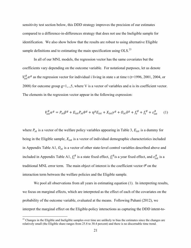
In all of our MNL models, the regression vector has the same covariates but the

coefficients vary depending on the outcome variable. For notational purposes, let us denote

as the regression vector for individual i living in state s at time t (t=1996, 2001, 2004, or

2008) for outcome group g=1,..,5, where V is a vector of variables and α is its coefficient vector.

The elements in the regression vector appear in the following expression:

ƞ (1)

where is a vector of the welfare policy variables appearing in Table 3, is a dummy for

being in the Eligible sample, is a vector of individual demographic characteristics included

in Appendix Table A1, is a vector of other state-level control variables described above and

included in Appendix Table A1, is a state fixed effect, is a year fixed effect, and is a

traditional MNL error term. The main object of interest is the coefficient vector θg on the

interaction term between the welfare policies and the Eligible sample.

We pool all observations from all years in estimating equation (1). In interpreting results,

we focus on marginal effects, which are interpreted as the effect of each of the covariates on the

probability of the outcome variable, evaluated at the means. Following Puhani (2012), we

interpret the marginal effect on the Eligible-policy interactions as capturing the DDD intent-to-

23 Changes in the Eligible and Ineligible samples over time are unlikely to bias the estimates since the changes are relatively small (the Eligible share ranges from 25.8 to 30.4 percent) and there is no discernable time trend.

22

treat effect.24 All specifications are estimated using sample weights and standard errors are

clustered by state.

IV. Main Results Tables 4 and 5 provide our main results. Table 4 provides the marginal effects from a

specification where each policy variable is included separately (our “unbundled” specification)

and Table 5 provides the marginal effects from our “bundled” policy specifications, one using

“any reform” variables and one using “number of” reforms variables. The marginal effects

associated with the other variables in the unbundled specification are presented in Appendix

Table A2.

We turn first to the unbundled results in Table 4. Overall, we find that most welfare

policies did not affect family structure. Indeed, a large majority of the coefficients are not

statistically significant at conventional levels. This lack of significance includes the effects of

family-related policies, which should have the most direct effects on family structure. For

example, not easing two parent rules did not encourage the creation of single-parent households

(or unrelated cohabiting) at the expense of two-parent biological households. Indeed, none of the

family-related policies appear to have had a major effect on family structure.25 These (lack of)

24 There has been some debate in the literature about computation of marginal effects, with Ai and Norton (2003) having argued that computing marginal effects in nonlinear models with interactions requires using all parameters of the model. However, Puhani (2012) has since argued that the application of the Ai-Norton approach to DD models violates the assumption of parallel trends in the treated and comparison groups--which is the main feature of such models--and argues that the marginal effect of the coefficient on the interaction term in DD models is the correct approach. See Karaca-Mandic, Norton, and Dowd (2012) for a non-technical discussion of this point. Many subsequent papers have used the Puhani approach (see, e.g. Ziebarth, 2010; Bargain et al., 2012; Ziebarth, 2013; Mayer et al, 2014, Weisburd, 2015; De Angelis et al., 2017) and we follow it as well. However, as a robustness check, we have also computed marginal effects as suggested by Ai and Norton (2003); the results are almost identical to those in Table 5 (available upon request). In addition, we estimate linear probability models (presented below) to test the robustness of our findings using a linear model. 25 While it is possible to speculate about the two significant findings obtained on unrelated cohabitation (see our previous discussion regarding family caps encouraging unrelated cohabiting), these findings are not robust to

23

findings corroborate the prior literature, which has also not found consistent or strong effects of

family-related welfare reform policies on family structure, albeit without the longer time frame

or the more precisely defined family structure measures used here.

At the same time, we do find evidence that some work-related waiver and TANF policies

significantly affected family structure. Table 4 shows that policies of not expanding disregards

(in both the waiver and TANF periods) and of imposing strict TANF sanctions significantly

increased the probability of being a single mother (by 2.2 to 4.3 percentage points) and the

former policies reduced the probability of marriage to biological partners (by 3.3 to 5.1

percentage points).26 As we show below, these results are quite robust.

The results also show a few statistically significant effects of work-related policies on

cohabitation – with some encouraging cohabitation while others discouraging it. For example,

we find that work requirement waivers and no expanded TANF disregard encouraged unrelated

cohabitation, and no expanded TANF disregard encouraged biological cohabitation. However,

we also find that strict TANF sanctions and strict TANF work exemptions discouraged unrelated

cohabitation and biological cohabitation, respectively. Thus, it does not appear that work-related

policies had a clear effect on cohabitation. This becomes even more evident in our bundled

results and robustness analysis, which follow.

As discussed previously, the interpretation of the effects of individual policies is

complicated by the simultaneity of policy changes associated with welfare reform. Therefore,

we present estimates in Table 5 of specifications that use our bundled policy variables, which

alternative specifications (see Table 7 below when 1993 is included) and so our general conclusion is that family-related policies do not, as whole, have much effect on family structure. 26 We note also that the effect of a Strict TANF Sanction on biological married is of the same sign and close to the magnitude of the effect of the No Expanded Disregard and only slightly below conventional significance levels. The effect of a Strict TANF Work Exemption and Sanction Waiver on single parent and biological married are, likewise, of the same sign and close to the magnitude of the other work-related policies.

24

may better capture the overall effect of adopting at least one policy or adopting a set of reforms

together. The results clearly indicate that work-related policies, in both the waiver period and

TANF period, lead to strong positive effects on single motherhood and negative effects on

biological marriage. These results are similar to those in Table 4, but the effects are sometimes

larger in magnitude (than the average of the policies in Table 4) and the standard errors decrease.

This is especially evident in the “number of reforms” specification. The coefficients imply that

each work related waiver policy increased single parenthood by 2.8 percentage points and

decreased biological marriage by 2.8 percentage points, while each strict work-related TANF

policy increased single parenthood by 1.5 percentage points and decreased biological marriage

by 1.8 percentage points. Lastly, Table 5 also shows that most of the significant coefficients in

Table 4 on cohabitation are not robust to specification, as noted previously.27

This pattern of results, with work-related welfare reforms increasing single motherhood

and decreasing marriage, has been found in some instances in the previous literature, although

the declines have been assigned to marriage as a whole, regardless of the father’s biological

relationship to the children. For example, Fraker et al. (2002) and Bitler et al. (2004b) found

statistically significant negative effects of welfare reform and work-related policies on marriage;

Dunifon et al. (2009) found some negative effects on the relative probability of children residing

in married households versus single-parent households; and Fitzgerald and Ribar (2004) found

positive effects of work-related polices on female headship in one specification.28 An important

difference of our analysis compared to past work is that we find that the significant negative

27 The coefficients on the bundled family-oriented policies also are almost all insignificant. See also n.25 above. 28 Bitler et al. (2004b) did find their marriage results to be sensitive to specification and choice of data, and Dunifon et al. (Table 7) found their negative effects for both white and black women for different specifications but concluded that they were not sufficiently robust across specifications to warrant confidence in the finding. Ellwood (2000) also found evidence of negative effects on welfare reform on marriage but of weak significance. Gennetian and Knox (2003), in a meta-analysis of 14 RCTs that were not always the same as the actual reforms implemented, found small negative effects on marriage for some subgroups for programs that combined time limits with expanded earnings disregards.

25

effect on marriage operates through marriage to biological fathers only, and not through marriage

to unrelated men.

The finding that work-related welfare reforms increased single motherhood or led to

marriage declines has been interpreted as resulting from what has been called the “independence

effect.” This interpretation is bolstered by the large literature on the effects of welfare reform on

employment and earnings of low income women, which finds that welfare reform caused large

declines in program participation coupled with gains in employment and earnings (Moffitt, 2003;

Ziliak, 2016). Indeed, when we analyze the effects of these policies on welfare participation and

the employment and earnings of our sample of Eligible mothers in the SIPP, we find that bundles

of work-related waivers and TANF policies discouraged welfare participation (Appendix Table

A3) and increased earnings (Appendix Table A4). However, why the independence effect might

be particularly strong in discouraging marriage to biological fathers is a separate question, which

we take up in Section V below, after we conduct extensions and sensitivity tests to ensure our

findings are robust.

Extensions. We conduct three important extensions to our main results. First, we

estimate our baseline specification using the linear probability model. This tests the sensitivity

of our results to the MNL model assumptions (nonlinear effects of the regressors, independence

of irrelevant alternatives, extreme value Type II error terms). Second, we extend the time period

back to 1993 to increase the number of pre-TANF periods. Third, we examine whether the

effects of these policies have changed over time.

Table 6 presents results from estimating simple linear probability models for each of our

five family structure outcomes, where the dependent variable is coded 1 if that outcome was

chosen and coded 0 if any of the other four outcomes were chosen. A few of the coefficients in

26

the unbundled specification are weaker than those in Tables 4, with smaller magnitudes and

lower significance levels, but most of the work-related policy effects retain their general

magnitudes and significance levels. The bundled specifications entirely retain the significance

levels found in Table 5. Once again, family-related policies have no effect. Thus the results

using OLS are very consistent with those of the MNL specification.

Table 7 presents the results when the analysis is extended to include 1993. Extending our

analysis back to 1993 poses some difficulties. Our definition of a cohabitor uses the “unmarried

partner” relationship designation. However, this option was not included as a relationship

designation until the 1996 SIPP. Thus, extending the data back to include the 1993 SIPP

requires us to alter our definition of a cohabitor. In this extension, we use the well-known

adjusted POSSLQ definition to identify cohabitors (Casper and Cohen, 2000),29 which is known

to be inferior to more direct questions (Baughman et al, 2002). As in our preferred definition of

cohabitation, we also included the sample of unmarried parents (two non-married adults with a

common biological child, identified via the HHRM in the 1993 SIPP, as in later panels) in our

definition of cohabitation.

We find that adding 1993 to our analysis causes no substantive changes to our results.

First, we estimate our models using the same 1996 to 2008 sample period but with the adjusted

POSSLQ-based definition of cohabitation. In results not shown, we find that our results in Table

4 and Table 5 are robust to the use of this alternative cohabitation definition. We then estimate

our models after adding 1993 to our 1996, 2001, 2004, and 2008 pooled sample and using our

29 The adjusted POSSLQ definition of cohabitation includes two unrelated, unmarried adults of the opposite sex that live together in a household where any other adult in the household is related to one of the unrelated, unmarried, opposite-sex adults.

27

new definition of cohabitation for all years.30 Importantly, the main results are essentially

unchanged from those reported in Tables 4 and 5. The estimated effects of work-related waiver

and TANF policies on single motherhood and biological marriage are almost identical for both

the unbundled and bundled specifications. Moreover, the estimated effects of work- and family-

related policies on cohabitation generally lack statistical significance, reinforcing our earlier

findings. The similarity in these estimates suggests that the 1996 data are, indeed, a pre-TANF

period.

Our third extension examines whether the effects of welfare policies on family structure

change with time after 1996. Family structure is likely to react more slowly to welfare reform

policies than work, which has been found to respond quickly to policy changes. Table 8 shows

our results when we estimate the “number of reforms” specifications using the 1996/2001 data,

the 1996/2004 data, and the 1996/2008 data (Appendix Table A5 presents these results for the

“any reform” specifications). The waiver-period year of 1996 must be included in each

regression to provide the baseline against which TANF effects are measured.

The results from this analysis are striking. In the 1996-2001 period, work-related polices

retain their significant positive effects on single motherhood but their effects on biological

marriage are no longer significant However, with each succeeding year, the positive effects on

single motherhood and on biological marriage grow in magnitude and in significance, reaching

their maximum values in 2008.31 This pattern suggests that the stronger effects we have found

for work-related policies on family structure, as compared to past studies, may be the result of

our inclusion of later years in the analysis.

30 Work-related waiver variables and family-related policy variables for 1993 were also added to the data set; these have been widely used in past work. 31 Using 1996 and 2004 data, an exception is the coefficient on the Number of Strict Work-Related TANF policies on single motherhood, which does not grow in magnitude and moves slightly below the cutoff for 10 percent significance. However, it returns to significance and grows in magnitude with 2008.

28

One interpretation of the strengthening effects on family structure is a cohort-based

explanation. Women who were older in 1996 may have already made decisions about marriage

and cohabitation (especially with the biological father of their children) and they may have been

slow to change or reverse those prior decisions after the arrival of welfare reform. With the

passage of time, however, younger cohorts arrive at the key partnering years (late teens, 20s)

with welfare reform permanently in place, and those cohorts were able to make decisions less

encumbered by past history.32 If this is the mechanism at work, the long-term effects of some

work-related policies on family structure could be quite different than their short-term effects.

Robustness and Sensitivity Tests. We conduct several robustness tests to check the

sensitivity of our results to alternative specifications. So far, we have shown that the effects of

work-related waiver and TANF policies on single motherhood and biological marriage are robust

to a limited number of extensions but the results for other family structure outcomes are not.

This section reports a larger number of robustness tests to determine whether both of these

conclusions remain after conducting those tests.

Table 9 presents the results of a large number of additional sensitivity tests to our main

MNL results (with control variables included). For brevity, we focus on sensitivity results for

the “number of reform” specification, however Appendix Table A6 repeats this analysis for the

“any reform” specification and we find similar results in those specifications as well as in the

unbundled specifications, which are available by request. In Table 9, Panel I reports our baseline

results from Table 5 for easy comparison. Panel II examines the sensitivity of the results to the

inclusion of an Ineligible group in our estimation by dropping the Ineligible sample entirely. In

this specification, the policy impacts are identified only from differences in family structure

32 In separate analyses not presented here, we find suggestive evidence that this is indeed taking place. We find that the estimated effects of these welfare rules on family structure tend to be larger and more pronounced on both younger cohorts and younger-aged (i.e. below median-age) mothers. These results are available by request.

29

outcomes over time across states as result of variation in welfare policies in the Eligible group

(and not relative to family structure changes over time in those states among Ineligible). The

results show that our four significant baseline results lose significance in three of those cases, but

the magnitudes of the coefficients are, in two of the three cases, only slightly weakened. We

take this as indicating that our main findings are present in the Eligible group but adding the

Ineligible group improves the precision of the estimates.

Panels III and IV test the sensitivity of the results to changes in the definition of the

Eligible/Ineligible groups. Panel III drops the automobile restriction for the Eligible group

(thereby allowing the Eligible sample to have any number of cars, as permitted in a few states).

The results show that the baseline effects of work-related policies on single parenthood and

biological marriage remain, with slightly altered magnitudes. The results also imply a significant

positive effect of work-related reforms on biological cohabiting but this coefficient is significant

in almost no other specification and hence is not robust. Panel IV excludes college graduates

from the Ineligible group, leaving the Ineligible sample defined only on the basis of high assets.

The results after this Ineligible definition change are virtually identical to the baseline results.

Panel V tests the sensitivity of our baseline results to the inclusion of separate time trends

by state, a common extension of the standard state fixed effects model. The baseline results are

again unaltered by this change. Panel VI tests the sensitivity of our results to the treatment of

blended households (i.e., households where some of the mother’s children are biological to the

male in the household and some are not), where our baseline model includes blended households

in with biological households rather than in with unrelated households. Our results are again

very similar to those in the baseline model. Lastly, Panel VII limits the sample to white, non-

Hispanic mothers to test for race-ethnic differences in our estimates. While the magnitudes of the

30

marginal effects are smaller in this specification, the estimated coefficients on work-related

policies follow the same pattern of effects and TANF work-related policies remain statistically

significant. Additionally, these smaller effects on white, non-Hispanic mothers are exactly what

we would expect if work-related policies indirectly affect family structure through the welfare

participation decision. Since white, non-Hispanic mothers are less likely to be on welfare (10.2

percent) than minority mothers (16.8 percent), the independence effect associated with welfare

reform should also be smaller.

V. Economic Characteristics of Male Partners

Our most robust finding is that combinations of work-related welfare reforms (in our

“number of” specifications) led to an increase in single motherhood and a decrease in marriage

to biological fathers. Our primary hypothesis to explain this change in family structure,

mentioned frequently in the literature, is that welfare reform led to an increase in female

employment and earnings which, through an independence effect, led to a decrease in partnering.

There is extensive evidence that welfare reform did indeed improve the average employment and

earnings outcomes of women (Moffitt, 2003; and Ziliak 2016), and we find similar effects of

work-related welfare policies on the sample of Eligible mothers in the SIPP (see Appendix Table

A4). However, an obvious question is why it would have led to a decrease in partnering

specifically through marriage to biological fathers and not to cohabitation with either biological

or unrelated fathers or to marriage to unrelated males, a question we investigate further here.

Theoretical models of the determinants of marriage, cohabitation, and single motherhood

in the economics literature have not considered the biological relationship of potential union

partners to a mother’s children. However, there is a large literature in demography on the

31

characteristics of men in unions, which distinguishes men exactly the way we have here—by

marital status and by biological relationship (Hofferth and Anderson, 2003; Cherlin and Fomby,

2005; Hofferth, 2006; Manning and Brown, 2006; Berger et al., 2008; Bzostek et al., 2012;

Kennedy and Fitch, 2012; and Carlson and Berger, 2013; among others). While this literature is

focused almost exclusively on the question of how the biological and marital status of men

affects child outcomes, these studies also examine male economic characteristics by different

biological/marital types. They largely indicate that the employment and earnings of married

biological fathers are the highest among all types of male partners (see, especially, Hofferth and

Anderson, 2003; Manning and Brown, 2006). Married unrelated men (i.e., stepfathers) are

typically ranked second highest, and cohabiting men of either biological status typically have the

weakest economic characteristics.

The employment and average earnings (conditional on employment) of male partners for

the Eligible sample of mothers are displayed in Figure 1. Consistent with past work, married

biological fathers typically have the highest levels of employment and earnings but they are not

always very far above those of stepfathers. Additionally, the employment and earnings of

cohabiting men are considerably lower. Among cohabiting men, unrelated cohabitors tend to

have higher employment rates and earnings levels than biological cohabiting fathers, as found in

Bzostek et al. (2012). A striking aspect of the figure is that the employment of all types of male

partners has been declining over time. This decline in labor market activity and wage rates

among lower skilled men in the U.S. over this period has been documented extensively

elsewhere, and has been variously ascribed to skill-biased technological change, international

trade, incarceration, health and disability, and a variety of other factors (Aaronson et al., 2006;

Moffitt, 2012; and Council of Economic Advisers, 2016). However, the rates of decline for men

32

classified by marital status and by the biological relationship with the children in the household

have not been examined.

Despite the stronger economic characteristics of biological fathers, we suggest three

possible reasons for a stronger negative effect on biological marriage than on other partner types.

The first reason is a simple utility-based explanation tied to the increase in mothers’ earnings

induced by welfare. The economic value of a union to a woman is, in the simplest of all models,

an increasing function of her earnings (Wf), her partner’s earnings (Wm), and the share of each

earnings amount that she gets to consume (sf and sm). This set-up leads to the following utility

function: U(sfWf+smWm). If U is concave, as generally supposed, then ∂U2/∂Wm∂Wf<0. This

implies that a woman gets less additional utility from a higher-earnings partner, the higher her

own earnings. Since biological married fathers have the highest earnings, their advantage would

fall the most subsequent to a reform that increases the level of female earnings.

A second, more mechanical hypothesis may simply stem from the fact that, of all partner

types, marriage to biological fathers is by far the most common type, constituting 75 percent of

all unions within the Eligible sample. A well-known characteristic of almost all cumulative

probability distribution functions is that they flatten out in the tails with respect to their index

functions. Therefore, changes in their determinants have much smaller effects at probabilities

close to 1 or 0 and much greater effects in the middle probability ranges.33 This means that

there may be more of an effect on marriage to biological fathers because that is where there are

enough unions to have effects in the first place.

33 In the probit model, for example, the effect of a change in X on the probability equals the normal density times the probit coefficient, and that density is at its maximum at a .50 probability and approaches zero in the tails. The effect in the logit model is the logit coefficient times p(1-p), where p is the probability, which has the same maximum and approach to zero as in probit.

33

A third possible explanation is that the employment and earnings among biological

married males may have declined faster among men in our Eligible sample than in our Ineligible

sample. Further, if this relative decline was larger for biological married men than for other

types of partners, then we would expect to see the largest relative effect among biological

married men in the Eligible group. The regression results in Table 10 show that this is indeed

the case. Pooling all observations on the male partners of the women in our sample over the

years 1996-2008, we estimate OLS regressions for the employment and real monthly earnings

(levels and logs, conditional on employment) for male partners on indicators for the partner types

and interactions between the partner types and an indicator for being a partner of a mother in our

Eligible sample. Specification 1 has interactions terms for all years combined while

Specification 2 furthers interact these partner type indicators for the overall and Eligible sample

with year indicator variables, albeit combining non-bio-married men into a single “other partner”

variable.34 The results show that biological married men experience the largest relative earnings

disadvantage vis-à-vis other partner types with average relative earnings differences of $650 per

month or 0.24 log points. Moreover, the disadvantage of Eligible biological married men

relative to Ineligible biological married men has grown over time. This is especially evident for

real earnings, where the relative earnings disadvantage for Eligible biological married males

increased from about $450 per month to $800 per month while there was essentially no change in

the relative disadvantage for other partner types. Biological married males in the Eligible sample

also experienced larger relative employment declines compared to the Ineligible sample than

other partner types: 3 percentage points versus 2 percentage points.

34 Both specifications also include state and year fixed effects, all of the demographic variables (Xist) from equation (1), and all other state-level (non-welfare) policies (Oist) from equation (1). The specifications do not include controls for any of our welfare rules and the earnings regressions are limited to employed individuals earning more than $0 and less than $15,000 per month.

34

These regression results are only suggestive of changes in male partner characteristics

because there are obvious selection effects that could be occurring over time. The wages and

employment of men in different union status types could be changing simply because men of

different economic characteristics are changing status categories, or moving into and out of

unions at different rates, for example. More generally, neither this hypothesis nor the other two

we have suggested for explaining our results for biological father unions is definitive, and a full

investigation of each must await future research.

VI. Conclusions

In this paper, we analyze the incentive effects of welfare reform using a definition of

family structure that more closely matches AFDC and TANF welfare rules regarding the

treatment of men in the household. We also examine the effects of welfare rules over a longer

period of time than any previous study, which allows us to distinguish between short-run and

long-run effects.

Consistent with prior work, we find that most welfare reform elements had no significant

effect on women’s family structure. However, we find robust evidence that some work-related

waivers and work-related TANF policies increased single motherhood and decreased marriage to

biological fathers. These results are evident when welfare reform policies are considered

individually but they are larger and of greater statistical significance when the policies are

considered jointly. While some studies in the literature have similarly found that work-related

reforms increased single parenthood and reduced marriage (Bitler et al., 2004; Dunifon et al.

2009; Ellwood, 2000; Fitzgerald and Ribar, 2004; Fraker, 2002; Gennetian and Knox, 2003),

these past findings have generally been of borderline significance or nonrobust to specification.

35

Further, our results show that the identified reductions are only for marriage to biological fathers

and the magnitude of these effects has been growing over time.

We offer some explanation, buttressed by additional analysis, for the results obtained.

Past research as well as evidence from our data suggests that welfare reform pushed women off

welfare and increased their employment and earnings, enabling them to better support

themselves without a male partner. This “independence effect” likely explains the increase in

single motherhood that we observe. Why the rise in single motherhood is associated with a

significant decrease in marriage to biological fathers but not other partners is an additional

question. We provide some suggestive evidence that the economic position of married biological

fathers in the Eligible sample has fallen the most relative to similar fathers in the Ineligible

sample, leading such men to be relatively less attractive. We offer other explanations for the

disproportionate decline in marriage to biological fathers as well.

Our findings suggest that other transfer programs that increase the labor market earnings

of women may also have important indirect effects on family structure. For example, while the

Earned Income Tax Credit (EITC) generally discourages marriage through the marriage penalty

associated with the tax code, it may further discourage marriage due to its positive effects on

female labor force participation and earnings. Moreover, our results, which show that these

indirect effects on family structure grow over time, point to the importance of estimating longer-

run effects of the EITC. To date, the evidence on the effects of the Earned Income Tax Credit on

marriage and divorce is mixed, with Dickert-Conlin and Houser (2002) finding no effect, while

Herbst (2011) finds small negative effects on marriage. Whether our results showing differential

effects on marriage and cohabitation by biological status extend to the EITC or other transfer

programs such as Medicaid is unknown, because the literature on family structure effects of

36

those programs has not distinguished unions by biological status of the male. 35 However, our

results suggest that future research on the family structure effects of other transfer programs

should carefully consider eligibility rules and may want to distinguish households by the

partner’s biological status.

Our results are also relevant to the recent proposals to transition the Supplemental

Nutritional Assistance Program (SNAP) and Medicaid program to block grants with work

requirements for recipients (e.g., Goodnough, 2018). These policy changes may have similar

effects in increasing women’s labor force participation and earnings, which could have important

indirect effects on family structure as we have observed from 1990s welfare reform.

35 There are a few studies on the effects of Medicaid on marriage and divorce in its early period (Decker, 2000; Yellowitz, 1998), but there have been no recent ones that we are aware of.

37

VI. References

Aaronson, S., B. Fallick, A. Figura, J. Pingle, and W. L. Wascher. 2006. “The Recent Decline in Labor Force Participation and its Implications for Potential Labor Supply.” Brookings Papers on Economic Activity, 1:2006. Acs, G. and S. Nelson. 2004. "Changes in Living Arrangements during the Late 1990s: Do Welfare Policies Matter?" Journal of Policy Analysis and Management 23(2): 273-90. Ai, C. and Norton, E.C. 2003. “Interaction Terms in Logit and Probit Models.” Economics Letters. 80(1): 123-129. Bargain, O., González, L., Keane, C. and Özcan, B. 2012. “Female Labor Supply and Divorce: New Evidence from Ireland.” European Economic Review. 56(8): 1675-1691. Baughman, R. S. Dickert-Conlin and S. Houser. 2002. “How Well Can We Track Cohabitation Using the SIPP? A Consideration of Direct and Inferred Measures.” Demography 39(2): 455-465. Becker, G.S. 1991. A Treatise on the Family. Second Edition. Cambridge, MA: Harvard University Press. Berger, L., M. Carlson, S. Bzostek, and C. Osborne. 2008. Parenting Practices of Resident Fathers: The Role of Marital and Biological Ties. Journal of Marriage and Family, 70(3), 625-639. Bitler, M.; J. Gelbach; and H. Hoynes. 2004a. “Has Welfare Reform Affected Children's Living Arrangements." Focus 23(2):14-19. Bitler, M.; J. Gelbach; and H. Hoynes. 2006. “Welfare Reform and Children's Living Arrangements." Journal of Human Resources 41(1):1-27. Bitler, M.; J. Gelbach; H. Hoynes; and M. Zavodny. 2004b. "The Impact of Welfare Reform on Marriage and Divorce." Demography 41 (2): 213-236. Blackburn, M. 2003. “The Effects of the Welfare System on Marital Dissolution.” Journal of Population Economics 16 (August): 477-500. Blank, R. 2002. “Evaluating Welfare Reform in the United States.” Journal of Economic Literature 40 (December): 1105-66. Blau, D. and W. van der Klaauw. 2013. "What Determines Family Structure?" Economic Inquiry 51(1):579-604. Blau, F.; L. Kahn; and J. Waldfogel. 2004. “The Impact of Welfare Benefits on Single Motherhood and Headship of Young Women.” Journal of Human Resources 39 (Spring): 382-

38

404. Brandon, Peter. 2007. “Mapping Children’s Living Arrangements with a Relationship Matrix,” in Sandra L. Hofferth and Lynne M. Casper, eds., Handbook of Measurement Issues in Family Research. Lawrence Erlbaum, Chapter 10. Bzostek, S. H., McLanahan, S. S., & Carlson, M. J. (2012). Mothers' Repartnering after a Nonmarital Birth. Social Forces 90(3): 817-841. Carlson, M. and L. Berger. 2013. “What Kids Get from Parents: Packages of Parental Involvement across Complex Family Forms.” Social Service Review 87(2), 213-249. Carlson, M., S. McLanahan, and P. England. 2004. “Union Formation in Fragile Families,” Demography 41 (2): 237-261. Casper, L. M. and P. N. Cohen. 2000. "How Does POSSLQ Measure up? Historical Estimates of Cohabitation." Demography 37(2): 237-245. Cherlin, A. J. and P. Fomby (2005). “Welfare, Work, and Changes in Mothers’ Living Arrangements in Low-Income Families.” Population Research and Policy Review 23 (5-6): 543-565. Council of Economic Advisers, “The Long-Term Decline in Prime-Age Male Labor Participation” (June 2016), https://obamawhitehouse.archives.gov. Crouse, G. 1999. “State Implementation of Major Changes to Welfare Policies, 1992 – 1998.” Washington, DC: ASPE, Department of Health and Human Services. De Angelis, D., G. Grullon, and S. Michenaud. 2017. “The Effects of Short-selling Threats on Incentive Contracts: Evidence from an Experiment.” The Review of Financial Studies. 30(5): 1627-1659. Decker, S. 2000. “Medicaid, AFDC, and Family Formation.” Applied Economics 32 (December): 1947-56. Dickert-Conlin, S. and S. Houser. 2002. “EITC and Marriage.” National Tax Journal 40: 25-39. Duncan, G. and S. Hoffman. 1990. “Welfare, Economic Opportunities and Out-of-Wedlock Births Among Black Teenager Girls.” Demography 27 (November): 519-535. Dunifon, R.; K. Hynes; and H. E. Peters. 2009. "State Welfare Policies and Children's Living Arrangements." Social Service Review 83 (3): 351-388. Ellwood, D. 2000. "The Impact of the Earned Income Tax Credit and Social Policy Reforms on Work, Marriage, and Living Arrangements." National Tax Journal, 53(4, Pt 2): 1063-1105.

39

Ellwood, D. and C. Jencks. 2001. “The Uneven Spread of Single Parent Families: What Do We Know? Where Do We Look for Answers?” In Social Inequality, ed. K.M. Neckerman, pp.3-77. New York: Russell Sage Foundation. Fields, J. 2001. Living Arrangements of Children: Fall 1996. Current Population Reports, P70-74. Washington: U.S. Census Bureau. Fitzgerald, J. and D. Ribar. 2004. "Welfare Reform and Female Headship." Demography 41(2): 189-212. Fraker, T.M., et al. 2002. “The Evaluation of Welfare Reform in Iowa.” Mathematica Policy Research: DEA-0699. Gennetian, L. and V. Knox. 2003. “Staying Single: The Effects of Welfare Reform Policies on Marriage and Cohabitation.” Next Generation Project Working Paper No. 13. New York: Manpower Demonstration Research Corporation. Goodnough, A. 2018. “Kentucky Rushes to Remake Medicaid as Other States Prepare to Follow.” New York Times (February 10, 2018). Grogger, J. and L. Karoly. 2005. Welfare Reform: Effects of a Decade of Change. Cambridge, MA: Harvard University Press. Herbst, C. 2011. “The Impact of the Earned Income Tax Credit on Marriage and Divorce: Evidence from Flow Data.” Population Research and Policy Review 30 (February): 101-28. Hofferth, S.L. (2006). Residential Father Family Type and Child Well-Being: Investment versus Selection. Demography 43 (1): 53-77. Hofferth, S., & Anderson, K. (2003). Are All Dads Equal? Biology versus Marriage as a Basis for Paternal Investment. Journal of Marriage and Family 65(1): 213 -232. Hoffman, S. and E. M. Foster. 2000. “AFDC Benefits and Nonmarital Births to Young Women.” Journal of Human Resources 35 (Spring 2000): 376-391. Karaca‐Mandic, P., Norton, E.C. and Dowd, B. 2012. “Interaction Terms in Nonlinear Models.” Health Services Research. 47 (1pt1): 255-274. Kennedy, S. and C. A. Fitch. 2012. “Measuring cohabiting families in the United States: Assessing the impact of new data from the Current Population Survey” Demography 49(4): 1479-1498. Lichter, D.; LeClere, F.; and D. McLaughlin. 1991. "Local Marriage Markets and the Marital Behavior of Black and White Women.” American Journal of Sociology 96 (January): 843-867. Lopoo, L. M. and K. M. Raissian. 2014. “U.S. Social Policy and Family Complexity,” The

40

Annals of the American Academy of Political and Social Science 654 (1): 213-230. Manning, W. D. and S. Brown. 2006. “Children’s Economic Well-Being in Married and Cohabiting Parent Families.” Journal of Marriage and Family 68: 345-362. Mayer, C., Morrison, E., Piskorski, T. and Gupta, A. 2014. “Mortgage Modification and Strategic Behavior: Evidence from a Legal Settlement with Countrywide.” American Economic Review 104(9): 2830-57. McLaughlin, D. and D. Lichter. 1997. “Poverty and the Marital Behavior of Young Women.” Journal of Marriage and the Family 59 (August): 582-594. Moffitt, R. 1998. “The Effect of Welfare on Marriage and Fertility: What Do We Know and What Do We Need to Know?” In Welfare, the Family, and Reproductive Behavior, ed. R. Moffitt. Washington: National Research Council. Moffitt R. 2003. “The Temporary Assistance to Needy Families Program” In The Economics of Means-Tested Programs, Chapter 5, ed. R.A. Moffitt. Chicago: University of Chicago Press. Moffitt, R. 2007. “Welfare Reform: The U.S. Experience.” Swedish Economic Policy Review 14(2): 11-47. Moffitt, R. 2012. “The Reversal of the Employment-Population Ratio in the 2000s: Facts and Explanations.” Brookings Papers on Economic Activity 2012(2): 201-264. Moffitt, R., R. Reville, and A. Winkler. 1994. “State AFDC Rules Regarding the Treatment of Cohabitors: 1993.” Social Security Bulletin 57 (Winter): 26-33. Moffitt, R., R. Reville, and A.Winkler. 1998. “Beyond Single Mothers: Cohabitation and Marriage in the AFDC Program.” Demography 35 (3): 259-278. Moffitt, R. A., R. T. Reville, A. E. Winkler, and J. M. Burstain. 2009. “Cohabitation and Marriage Rules in State TANF Programs.” RAND Working Paper, WR-585-1.

Moffitt, R. and M. Ver Ploeg, eds. Evaluating Welfare Reform in an Era of Transition. National Academies Press, 2001.

Primus, W. E. and J. Beeson. 2002. "Safety Net Programs, Marriage, and Cohabitation." In Just Living Together: Implications of Cohabitation on Children, Families and Social Policy, ed. A. Booth and A. Crouter. Mahwah, NJ: Lawrence Erlbaum Assoc, Inc., 170-205.

Puhani, P.A. 2012. “The Treatment Effect, The Cross Difference, and the Interaction Term in Nonlinear “Difference-in-Differences” Models.” Economics Letters 115(1): 85-87.

41

Rosewater, A. Setting the Baseline: A Report on State Welfare Waiver (Washington, DC: Office of the Assistance Secretary for Planning and Evaluation, June 1, 1997), accessed 1/17/2014 from http://aspe.hhs.gov Urban Institute, Welfare Rules Database. Weisburd S. 2015. “Identifying Moral Hazard in Car Insurance Contracts.” Review of Economics and Statistics. 97(2):301-313. Winkler, A. 1995. “Does AFDC-UP Encourage Two-Parent Families?” Journal of Policy Analysis and Management 14 (1): 4-24. Yelowitz, A. 1998. “Will Extending Medicaid to Two-Parent Families Encourage Marriage?” Journal of Human Resources 33: 833-65. Ziebarth, N.R. 2010. “Estimating Price Elasticities of Convalescent Care Programmes.” The Economic Journal, 120(545): 816-844. Ziebarth, N.R. 2013. “Long-term Absenteeism and Moral Hazard—Evidence from a Natural Experiment.” Labour Economics. 24: 277-292. Ziliak, J. P. 2016. “The Temporary Assistance for Needy Families Program” In The Economics of Means-Tested Programs, volume 1. ed. R.A. Moffitt. Chicago: University of Chicago Press.

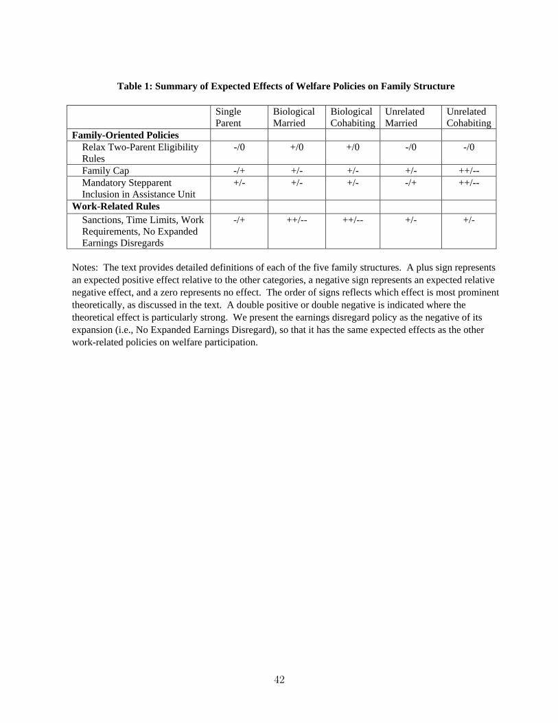
Table 1: Summary of Expected Effects of Welfare Policies on Family Structure

Single Parent

Biological Married

Biological Cohabiting

Unrelated Married

Unrelated Cohabiting

Family-Oriented Policies Relax Two-Parent Eligibility Rules

-/0 +/0 +/0 -/0 -/0

Family Cap -/+ +/- +/- +/- ++/-- Mandatory Stepparent Inclusion in Assistance Unit

+/- +/- +/- -/+ ++/--

Work-Related Rules Sanctions, Time Limits, Work Requirements, No Expanded Earnings Disregards

-/+ ++/-- ++/-- +/- +/-

Notes: The text provides detailed definitions of each of the five family structures. A plus sign represents an expected positive effect relative to the other categories, a negative sign represents an expected relative negative effect, and a zero represents no effect. The order of signs reflects which effect is most prominent theoretically, as discussed in the text. A double positive or double negative is indicated where the theoretical effect is particularly strong. We present the earnings disregard policy as the negative of its expansion (i.e., No Expanded Earnings Disregard), so that it has the same expected effects as the other work-related policies on welfare participation.  

42

Table 2: Family Structure of Mothers in the SIPPPercent Distribution in each Sample

WelfareEligible Ineligible FullSample Sample Sample

Biological Partner 45.1 78.5 69.2Biological Married 38.7 76.1 65.7Biological Cohabiting 6.4 2.4 3.5

Unrelated Partner 6.3 6.4 6.3Unrelated Married 3.5 4.8 4.4Unrelated Cohabiting 2.8 1.6 1.9

Single Parent 48.6 15.1 24.4

Welfare Participation Rate 14.0 1.3 4.9

N 13,828 33,900 47,728Notes: The figures are for the years 1996, 2001, 2004, and2008 pooled together. The full sample (eligible and ineligible)consists of women aged 18-55 with at least one biological child(aged 17 or younger) living in the household. The eligiblesample includes those mothers with less than 16 years of edu-cation who have limited assets, where limited assets are definedas: do not own any financial assets (stocks, bonds, etc.), donot own a retirement account, have under $3000 in the bank,or reside in a household that owns fewer than two cars. Theineligible sample include all college educated mothers and allnon-college educated mothers with asset levels that exceed theaforementioned asset restrictions. Welfare is defined as havingreceived positive AFDC (1996) or TANF (2001, 2004, 2008)income in the month prior to interview. “Biological” and“Unrelated” refer to the male’s biological relationship to thechild/children in the household. All means are weighted usingthe SIPP sample weights, pooled over all four years.

43

Table 3: State Welfare Policy Variables Used in the Analysis

Variable Name Definition/Measurement 1996 2001 2004 2008

Work-Related Waiver Policies1

Sanctions Statewide policy of sanctions (full or partial) on unit’s benefits 0.23 0.00 0.00 0.00Work Requirement Statewide time limit that triggers a work requirement 0.19 0.00 0.00 0.00No Expanded Disregard No statewide policy to expand the earned income disregard 0.75 0.00 0.00 0.00

Any Work-Related Waiver Policy2 Is either a sanction or work requirement waiver in place? 0.40 0.00 0.00 0.00Number of Work-Related Waiver Policies Sum (feasible range is 0 to 3, actual range is 1 to 2) 1.17 0.00 0.00 0.00

Strict Work-Related TANF Policies3

Strict Sanction Most severe sanction; case closed or unit’s benefit cancelled 0.00 0.59 0.61 0.76Strict Time Limit Time limit < median across all states (60 months) 0.00 0.14 0.12 0.14Strict Work Exemption Strict work exemption associated with age of child; child’s age 0.00 0.40 0.41 0.45

less than median across all states (12 months)No Expanded Disregard Earnings disregard not increased over period 0.00 0.25 0.22 0.20

Any Strict Work-Related TANF Policy Are any (of the above) strict TANF policies in place? 0.00 0.73 0.75 0.86Number of Work-Related Strict TANF Policies Sum (feasible range is 0 to 4, actual range is 0 to 4) 0.00 1.39 1.37 1.55

Family-Related Policies4

Family Cap State has “family cap” policy on benefits 0.21 0.55 0.52 0.50No Easing Two-Parent Rule State didn’t ease any aspect of any two-parent rule (work history 0.87 0.08 0.07 0.08

requirement, waiting period, or 100 hour rule)Stepparent Included5 State requires the inclusion of the stepparent in the assistance unit 0.17 0.21 0.23 0.21

Any Family-Related Policy Are any (of the above) family-related policies in place? 0.96 0.71 0.68 0.65Number of Family-Related Policies Sum (feasible range is 0 to 3, actual range is 0 to 2) 1.26 0.84 0.81 0.79

Notes: All values are mean values weighted using samples weights for the eligible sample.1 If implemented by December 1995 for 1996 values. All values equal to zero (by definition) in 2001, 2004, and 2008. Data from Crouse (1999).2 Any Work-Related Waiver Policy excludes the No Expanded Disregard Waiver because otherwise the Any Work-Related Waiver Policy variableis not identified (equal to one in all states in 1996 and zero in all states in all other years).3 By definition, the 1996 values are equal to zero. If enacted by 2000 for 2001 values, 2003 for 2004 values, and 2007 for 2008 values. Data fromUrban Institute’s Welfare Rules Database (WRD).4 If implemented by 1995 for 1996 values, 2000 for 2001 values, 2003 for 2004 values, and 2007 for 2008 values for all policies except Stepparentrules in 1996 are as of 1996. Data from Urban Institute’s WRD, except Family Cap and No Easing Two-Parent Rule in 1995 are fromCrouse (1999) and Rosewater (1997), respectively.5 The omitted category is stepparent is excluded from the assistance unit or the inclusion is optional.

44

Table 4: Welfare Policies and Five Category Family StructureMultinomial Logit Marginal Effects

Single Biological Biological Unrelated UnrelatedParent Married Cohabiting Married Cohabiting

Work-Related Waiver PoliciesSanction Waiver 0.026 -0.020 0.009 -0.005 -0.009

(0.021) (0.017) (0.011) (0.008) (0.007)

Work Requirement Waiver -0.037 0.009 0.000 0.008 0.020***(0.038) (0.027) (0.015) (0.007) (0.006)

No Expanded Disregard Waiver 0.043** -0.051*** 0.002 0.005 0.001(0.018) (0.019) (0.008) (0.006) (0.005)

Strict Work-Related TANF PoliciesStrict TANF Sanction 0.028** -0.026 0.004 -0.001 -0.005*

(0.013) (0.017) (0.004) (0.008) (0.003)

Strict TANF Time Limit -0.005 0.008 0.004 -0.008 0.001(0.016) (0.017) (0.005) (0.006) (0.003)

Strict TANF Work Exemption 0.015 -0.017 -0.008* 0.010 -0.001(0.010) (0.012) (0.004) (0.006) (0.002)

No Expanded Disregard TANF 0.022** -0.033** 0.010*** -0.006 0.007***(0.011) (0.014) (0.003) (0.006) (0.002)

Family-Related PoliciesFamily Cap -0.007 0.002 -0.004 0.002 0.006***

(0.009) (0.011) (0.004) (0.006) (0.002)

No Easing Two-Parent Rule 0.012 -0.002 0.000 0.001 -0.011***(0.018) (0.019) (0.006) (0.006) (0.004)

Stepparent Included 0.011 -0.025 0.004 0.007 0.003(0.015) (0.016) (0.004) (0.006) (0.003)

Notes: The marginal effects for the other control variables from this specification are shown inAppendix Table A2. Standard errors are clustered at the state-level and presented in parenthesesunder the coefficients. N = 47, 728. * p<0.1; ** p<0.05; and *** p<0.01.

45

Table 5: Welfare Policies and Five Category Family Structure, Bundled PoliciesMultinomial Logit Marginal Effects

Single Biological Biological Unrelated UnrelatedParent Married Cohabiting Married Cohabiting

“Any” Policy Specification

Any Work-Related Waiver Policy -0.005 -0.013 0.010* 0.006 0.002(0.018) (0.011) (0.006) (0.007) (0.005)

No Expanded Disregard Waiver 0.058*** -0.052*** 0.002 0.006 -0.014***(0.013) (0.013) (0.007) (0.007) (0.004)

Any Strict Work-Related TANF Policy 0.039*** -0.049*** 0.003 0.010 -0.003(0.009) (0.009) (0.004) (0.006) (0.002)

Any Family-Related Policy 0.005 -0.016 -0.001 0.004 0.008***(0.011) (0.013) (0.006) (0.008) (0.002)

“Number of” Policy Specification

Number of Work-Related Waiver Policies 0.028*** -0.028*** 0.005 -0.001 -0.004(0.010) (0.009) (0.005) (0.005) (0.003)

Number of Strict Work-Related TANF Policies 0.015*** -0.018*** 0.002 0.000 0.001(0.006) (0.006) (0.002) (0.002) (0.001)

Number of Family-Related Policies -0.002 -0.005 -0.001 0.005 0.003(0.010) (0.011) (0.004) (0.004) (0.002)

Notes: In the “Any” policy specification, we break out No Expanded Disregard Waiver from the Any Work-RelatedWaiver variable because this is necessary for identification, i.e. all states implemented a waiver policy as we havedefined them. The marginal effects for the other control variables from the unbundled specification are shown inAppendix Table A2. Standard errors errors are clustered at the state-level and presented in parentheses under thecoefficients. N = 47, 728. * p<0.1; ** p<0.05; and *** p<0.01.

46

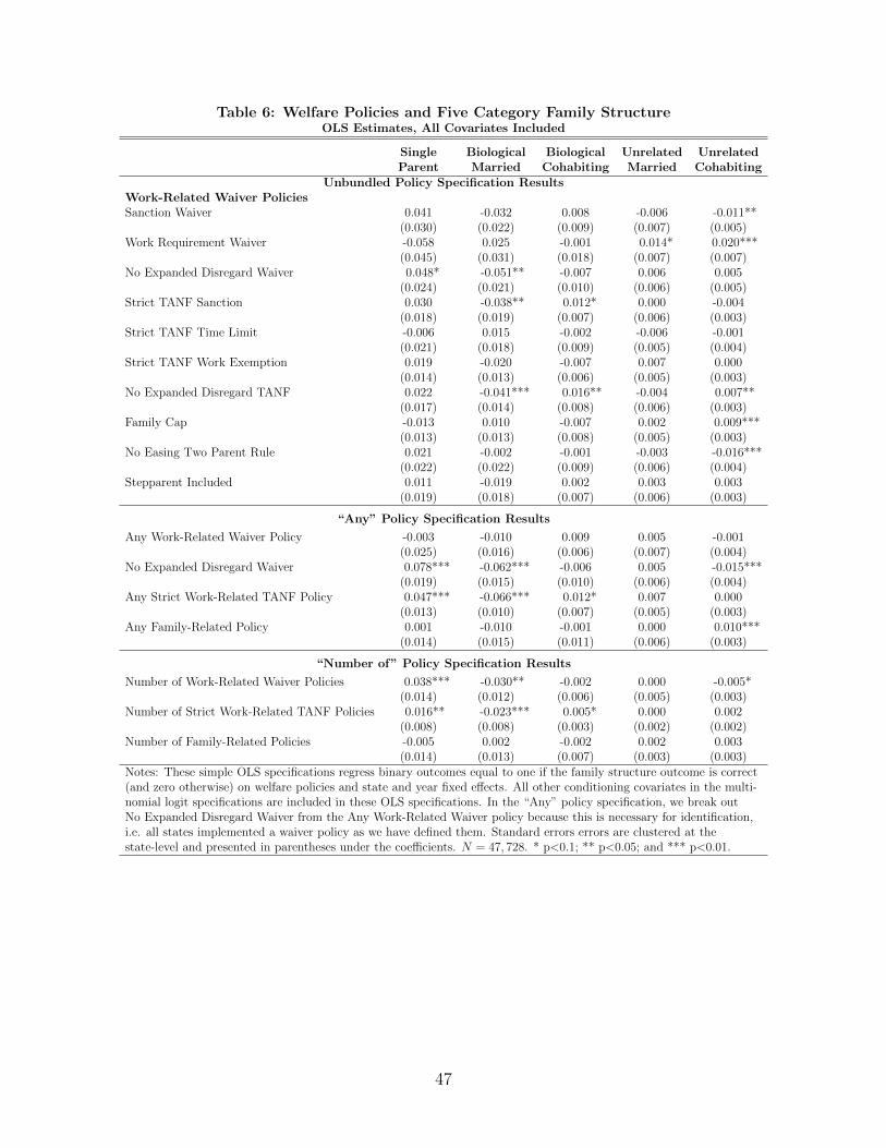
Table 6: Welfare Policies and Five Category Family StructureOLS Estimates, All Covariates Included

Single Biological Biological Unrelated UnrelatedParent Married Cohabiting Married Cohabiting

Unbundled Policy Specification ResultsWork-Related Waiver PoliciesSanction Waiver 0.041 -0.032 0.008 -0.006 -0.011**

(0.030) (0.022) (0.009) (0.007) (0.005)Work Requirement Waiver -0.058 0.025 -0.001 0.014* 0.020***

(0.045) (0.031) (0.018) (0.007) (0.007)No Expanded Disregard Waiver 0.048* -0.051** -0.007 0.006 0.005

(0.024) (0.021) (0.010) (0.006) (0.005)Strict TANF Sanction 0.030 -0.038** 0.012* 0.000 -0.004

(0.018) (0.019) (0.007) (0.006) (0.003)Strict TANF Time Limit -0.006 0.015 -0.002 -0.006 -0.001

(0.021) (0.018) (0.009) (0.005) (0.004)Strict TANF Work Exemption 0.019 -0.020 -0.007 0.007 0.000

(0.014) (0.013) (0.006) (0.005) (0.003)No Expanded Disregard TANF 0.022 -0.041*** 0.016** -0.004 0.007**

(0.017) (0.014) (0.008) (0.006) (0.003)Family Cap -0.013 0.010 -0.007 0.002 0.009***

(0.013) (0.013) (0.008) (0.005) (0.003)No Easing Two Parent Rule 0.021 -0.002 -0.001 -0.003 -0.016***

(0.022) (0.022) (0.009) (0.006) (0.004)Stepparent Included 0.011 -0.019 0.002 0.003 0.003

(0.019) (0.018) (0.007) (0.006) (0.003)

“Any” Policy Specification Results

Any Work-Related Waiver Policy -0.003 -0.010 0.009 0.005 -0.001(0.025) (0.016) (0.006) (0.007) (0.004)

No Expanded Disregard Waiver 0.078*** -0.062*** -0.006 0.005 -0.015***(0.019) (0.015) (0.010) (0.006) (0.004)

Any Strict Work-Related TANF Policy 0.047*** -0.066*** 0.012* 0.007 0.000(0.013) (0.010) (0.007) (0.005) (0.003)

Any Family-Related Policy 0.001 -0.010 -0.001 0.000 0.010***(0.014) (0.015) (0.011) (0.006) (0.003)

“Number of” Policy Specification Results

Number of Work-Related Waiver Policies 0.038*** -0.030** -0.002 0.000 -0.005*(0.014) (0.012) (0.006) (0.005) (0.003)

Number of Strict Work-Related TANF Policies 0.016** -0.023*** 0.005* 0.000 0.002(0.008) (0.008) (0.003) (0.002) (0.002)

Number of Family-Related Policies -0.005 0.002 -0.002 0.002 0.003(0.014) (0.013) (0.007) (0.003) (0.003)

Notes: These simple OLS specifications regress binary outcomes equal to one if the family structure outcome is correct(and zero otherwise) on welfare policies and state and year fixed effects. All other conditioning covariates in the multi-nomial logit specifications are included in these OLS specifications. In the “Any” policy specification, we break outNo Expanded Disregard Waiver from the Any Work-Related Waiver policy because this is necessary for identification,i.e. all states implemented a waiver policy as we have defined them. Standard errors errors are clustered at thestate-level and presented in parentheses under the coefficients. N = 47, 728. * p<0.1; ** p<0.05; and *** p<0.01.

47

Table 7: Welfare Policies and Five Category Family Structure, Including 1993 DataMultinomial Logit Marginal Effects

Single Biological Biological Unrelated UnrelatedParent Married Cohabiting Married Cohabiting

Unbundled Policy Specification ResultsWork-Related Waiver PoliciesSanction Waiver 0.024 -0.022 0.007 -0.006 -0.003

(0.024) (0.016) (0.009) (0.007) (0.005)

Work Requirement Waiver -0.037 0.018 0.001 0.011* 0.008(0.038) (0.025) (0.014) (0.006) (0.006)

No Expanded Disregard Waiver 0.042*** -0.048*** 0.006 0.002 -0.002(0.014) (0.014) (0.006) (0.006) (0.005)

Strict Work-Related TANF PoliciesStrict TANF Sanction 0.030** -0.022 0.002 -0.003 -0.008***

(0.012) (0.018) (0.004) (0.008) (0.003)

Strict TANF Time Limit -0.005 0.008 0.003 -0.009 0.002(0.015) (0.016) (0.005) (0.006) (0.003)

Strict TANF Work Exemption 0.013 -0.016 -0.007* 0.011* -0.001(0.009) (0.012) (0.004) (0.007) (0.003)

No Expanded Disregard TANF 0.024** -0.032** 0.009*** -0.006 0.005(0.011) (0.014) (0.003) (0.006) (0.003)

Family-Related PoliciesFamily Cap -0.009 0.004 -0.003 0.003 0.004

(0.009) (0.011) (0.004) (0.005) (0.003)

No Easing Two-Parent Rule 0.010 -0.003 -0.001 -0.002 -0.004(0.012) (0.013) (0.005) (0.005) (0.004)

Stepparent Included 0.011 -0.029* 0.004 0.009 0.005(0.015) (0.015) (0.004) (0.007) (0.004)

“Any” Policy Specification Results

Any Work-Related Waiver Policy -0.007 -0.008 0.008 0.006 0.002(0.019) (0.010) (0.005) (0.006) (0.004)

No Expanded Disregard Waiver 0.052*** -0.051*** 0.005 0.002 -0.008*(0.013) (0.011) (0.006) (0.006) (0.004)

Any Strict Work-Related TANF Policy 0.036*** -0.043*** 0.001 0.009 -0.003(0.010) (0.009) (0.004) (0.006) (0.003)

Any Family-Related Policy 0.004 -0.013 -0.001 0.004 0.007**(0.012) (0.014) (0.005) (0.008) (0.003)

“Number of” Policy Specification Results

Number of Work-Related Waiver Policies 0.030*** -0.031*** 0.006 -0.003 -0.002(0.010) (0.009) (0.004) (0.004) (0.003)

Number of Strict Work-Related TANF Policies 0.014*** -0.016*** 0.001 0.000 0.000(0.005) (0.006) (0.002) (0.002) (0.001)

Number of Family-Related Policies -0.002 -0.005 -0.001 0.005 0.003(0.010) (0.011) (0.003) (0.004) (0.002)

Notes: In the “Any” policy specification, we break out No Expanded Disregard Waiver from the Any Work-RelatedWaiver policy because this is necessary for identification, i.e. all states implemented a waiver policy as we havedefined them. The marginal effects for the other control variables for the 1996-2008 sample and the unbundledspecification are shown in Appendix Table A2. Standard errors are clustered at the state-level and presentedin parentheses under the coefficients. N = 54, 045, reflecting the pooled 1993, 1996, 2001, 2004, and 2008 samples.*p<0.1; ** p<0.05; and *** p<0.01.

48

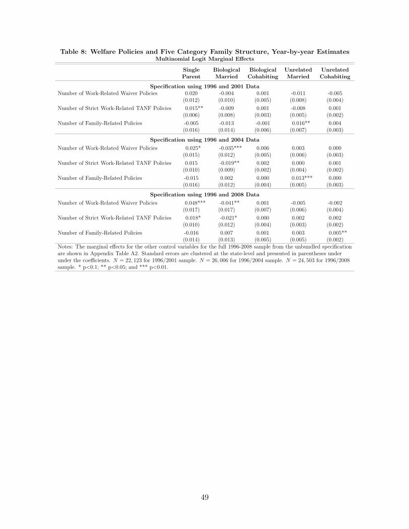
Table 8: Welfare Policies and Five Category Family Structure, Year-by-year EstimatesMultinomial Logit Marginal Effects

Single Biological Biological Unrelated UnrelatedParent Married Cohabiting Married Cohabiting

Specification using 1996 and 2001 DataNumber of Work-Related Waiver Policies 0.020 -0.004 0.001 -0.011 -0.005

(0.012) (0.010) (0.005) (0.008) (0.004)

Number of Strict Work-Related TANF Policies 0.015** -0.009 0.001 -0.008 0.001(0.006) (0.008) (0.003) (0.005) (0.002)

Number of Family-Related Policies -0.005 -0.013 -0.001 0.016** 0.004(0.016) (0.014) (0.006) (0.007) (0.003)

Specification using 1996 and 2004 Data

Number of Work-Related Waiver Policies 0.025* -0.035*** 0.006 0.003 0.000(0.015) (0.012) (0.005) (0.006) (0.003)

Number of Strict Work-Related TANF Policies 0.015 -0.019** 0.002 0.000 0.001(0.010) (0.009) (0.002) (0.004) (0.002)

Number of Family-Related Policies -0.015 0.002 0.000 0.013*** 0.000(0.016) (0.012) (0.004) (0.005) (0.003)

Specification using 1996 and 2008 Data

Number of Work-Related Waiver Policies 0.048*** -0.041** 0.001 -0.005 -0.002(0.017) (0.017) (0.007) (0.006) (0.004)

Number of Strict Work-Related TANF Policies 0.018* -0.021* 0.000 0.002 0.002(0.010) (0.012) (0.004) (0.003) (0.002)

Number of Family-Related Policies -0.016 0.007 0.001 0.003 0.005**(0.014) (0.013) (0.005) (0.005) (0.002)

Notes: The marginal effects for the other control variables for the full 1996-2008 sample from the unbundled specificationare shown in Appendix Table A2. Standard errors are clustered at the state-level and presented in parentheses underunder the coefficients. N = 22, 123 for 1996/2001 sample. N = 26, 006 for 1996/2004 sample. N = 24, 503 for 1996/2008sample. * p<0.1; ** p<0.05; and *** p<0.01.

49

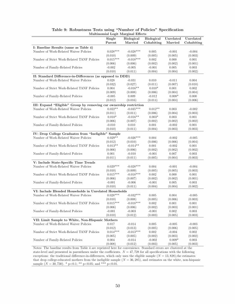
Table 9: Robustness Tests using “Number of Policies” SpecificationMultinomial Logit Marginal Effects

Single Biological Biological Unrelated UnrelatedParent Married Cohabiting Married Cohabiting

I: Baseline Results (same as Table 4)Number of Work-Related Waiver Policies 0.028*** -0.028*** 0.005 -0.001 -0.004

(0.010) (0.009) (0.005) (0.005) (0.003)Number of Strict Work-Related TANF Policies 0.015*** -0.018*** 0.002 0.000 0.001

(0.006) (0.006) (0.002) (0.002) (0.001)Number of Family-Related Policies -0.002 -0.005 -0.001 0.005 0.003

(0.010) (0.011) (0.004) (0.004) (0.002)

II: Standard Difference-in-Differences (as opposed to DDD)Number of Work-Related Waiver Policies 0.028 -0.031 0.010 -0.011 0.004

(0.032) (0.027) (0.011) (0.007) (0.010)Number of Strict Work-Related TANF Policies 0.004 -0.016** 0.010* 0.001 0.002

(0.009) (0.008) (0.006) (0.004) (0.004)Number of Family-Related Policies -0.005 0.009 -0.012 0.008* 0.000

(0.012) (0.016) (0.014) (0.004) (0.006)

III: Expand “Eligible” Group by removing car ownership restrictionNumber of Work-Related Waiver Policies 0.022** -0.035*** 0.012** 0.003 -0.002

(0.011) (0.011) (0.006) (0.004) (0.003)Number of Strict Work-Related TANF Policies 0.010* -0.016** 0.003* 0.003 0.001

(0.006) (0.007) (0.002) (0.002) (0.002)Number of Family-Related Policies -0.010 0.010 0.001 -0.002 0.001

(0.010) (0.011) (0.004) (0.003) (0.003)

IV: Drop College Graduates from “Ineligible” SampleNumber of Work-Related Waiver Policies 0.029** -0.026*** 0.004 -0.002 -0.005

(0.012) (0.010) (0.006) (0.006) (0.004)Number of Strict Work-Related TANF Policies 0.013** -0.014** 0.001 -0.002 0.001

(0.006) (0.006) (0.002) (0.002) (0.002)Number of Family-Related Policies 0.001 -0.010 -0.001 0.007 0.003

(0.011) (0.011) (0.005) (0.004) (0.003)

V: Include State-Specific Time TrendsNumber of Work-Related Waiver Policies 0.029*** -0.028*** 0.004 -0.001 -0.004

(0.010) (0.009) (0.005) (0.005) (0.003)Number of Strict Work-Related TANF Policies 0.015*** -0.018*** 0.002 0.000 0.001

(0.006) (0.007) (0.002) (0.002) (0.001)Number of Family-Related Policies -0.001 -0.006 -0.001 0.005 0.003

(0.010) (0.011) (0.004) (0.004) (0.002)

VI: Include Blended Households in Unrelated HouseholdsNumber of Work-Related Waiver Policies 0.028*** -0.032*** 0.005 0.004 -0.005

(0.010) (0.008) (0.005) (0.006) (0.003)Number of Strict Work-Related TANF Policies 0.015*** -0.018*** 0.002 0.001 0.001

(0.006) (0.006) (0.002) (0.003) (0.001)Number of Family-Related Policies -0.001 -0.003 -0.001 0.002 0.003

(0.010) (0.012) (0.003) (0.005) (0.003)

VII: Limit Sample to White, Non-Hispanic MothersNumber of Work-Related Waiver Policies 0.017 -0.014 0.005 -0.005 -0.003

(0.012) (0.013) (0.005) (0.006) (0.005)Number of Strict Work-Related TANF Policies 0.014*** -0.013*** 0.002 -0.004 0.002

(0.005) (0.005) (0.002) (0.003) (0.002)Number of Family-Related Policies 0.004 -0.014 -0.002 0.009* 0.003

(0.008) (0.012) (0.003) (0.005) (0.003)Notes: The baseline results from Table 4 are reprinted here for convenience. Standard errors are clustered at thestate-level and presented in parentheses under the coefficients. N = 47, 728 for all specifications with the followingexceptions: the traditional difference-in-differences, which only uses the eligible sample (N = 13, 828),the estimatesthat drop college-educated mothers from the ineligible sample (N = 36, 285), and estimates on the white, non-hispanicsample (N = 30, 730). * p<0.1; ** p<0.05; and *** p<0.01.

50

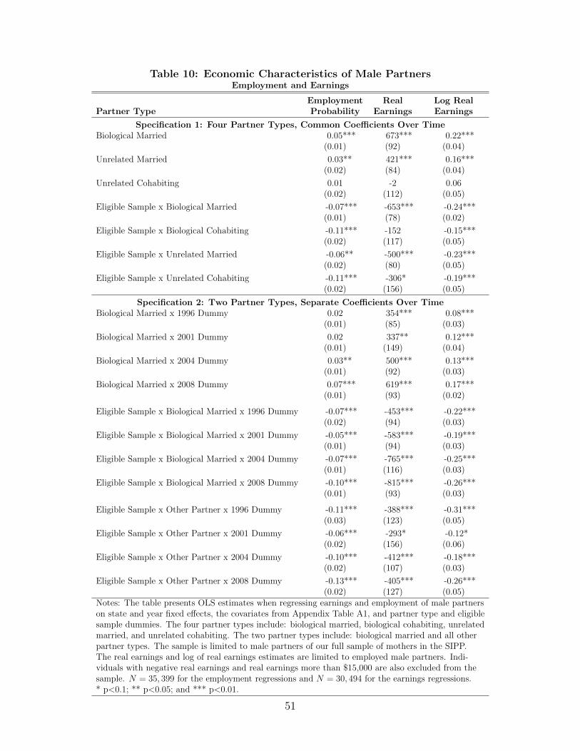
Table 10: Economic Characteristics of Male PartnersEmployment and Earnings

Employment Real Log RealPartner Type Probability Earnings Earnings

Specification 1: Four Partner Types, Common Coefficients Over TimeBiological Married 0.05*** 673*** 0.22***

(0.01) (92) (0.04)

Unrelated Married 0.03** 421*** 0.16***(0.02) (84) (0.04)

Unrelated Cohabiting 0.01 -2 0.06(0.02) (112) (0.05)

Eligible Sample x Biological Married -0.07*** -653*** -0.24***(0.01) (78) (0.02)

Eligible Sample x Biological Cohabiting -0.11*** -152 -0.15***(0.02) (117) (0.05)

Eligible Sample x Unrelated Married -0.06** -500*** -0.23***(0.02) (80) (0.05)

Eligible Sample x Unrelated Cohabiting -0.11*** -306* -0.19***(0.02) (156) (0.05)

Specification 2: Two Partner Types, Separate Coefficients Over TimeBiological Married x 1996 Dummy 0.02 354*** 0.08***

(0.01) (85) (0.03)

Biological Married x 2001 Dummy 0.02 337** 0.12***(0.01) (149) (0.04)

Biological Married x 2004 Dummy 0.03** 500*** 0.13***(0.01) (92) (0.03)

Biological Married x 2008 Dummy 0.07*** 619*** 0.17***(0.01) (93) (0.02)

Eligible Sample x Biological Married x 1996 Dummy -0.07*** -453*** -0.22***(0.02) (94) (0.03)

Eligible Sample x Biological Married x 2001 Dummy -0.05*** -583*** -0.19***(0.01) (94) (0.03)

Eligible Sample x Biological Married x 2004 Dummy -0.07*** -765*** -0.25***(0.01) (116) (0.03)

Eligible Sample x Biological Married x 2008 Dummy -0.10*** -815*** -0.26***(0.01) (93) (0.03)

Eligible Sample x Other Partner x 1996 Dummy -0.11*** -388*** -0.31***(0.03) (123) (0.05)

Eligible Sample x Other Partner x 2001 Dummy -0.06*** -293* -0.12*(0.02) (156) (0.06)

Eligible Sample x Other Partner x 2004 Dummy -0.10*** -412*** -0.18***(0.02) (107) (0.03)

Eligible Sample x Other Partner x 2008 Dummy -0.13*** -405*** -0.26***(0.02) (127) (0.05)

Notes: The table presents OLS estimates when regressing earnings and employment of male partnerson state and year fixed effects, the covariates from Appendix Table A1, and partner type and eligiblesample dummies. The four partner types include: biological married, biological cohabiting, unrelatedmarried, and unrelated cohabiting. The two partner types include: biological married and all otherpartner types. The sample is limited to male partners of our full sample of mothers in the SIPP.The real earnings and log of real earnings estimates are limited to employed male partners. Indi-viduals with negative real earnings and real earnings more than $15,000 are also excluded from thesample. N = 35, 399 for the employment regressions and N = 30, 494 for the earnings regressions.* p<0.1; ** p<0.05; and *** p<0.01.

51

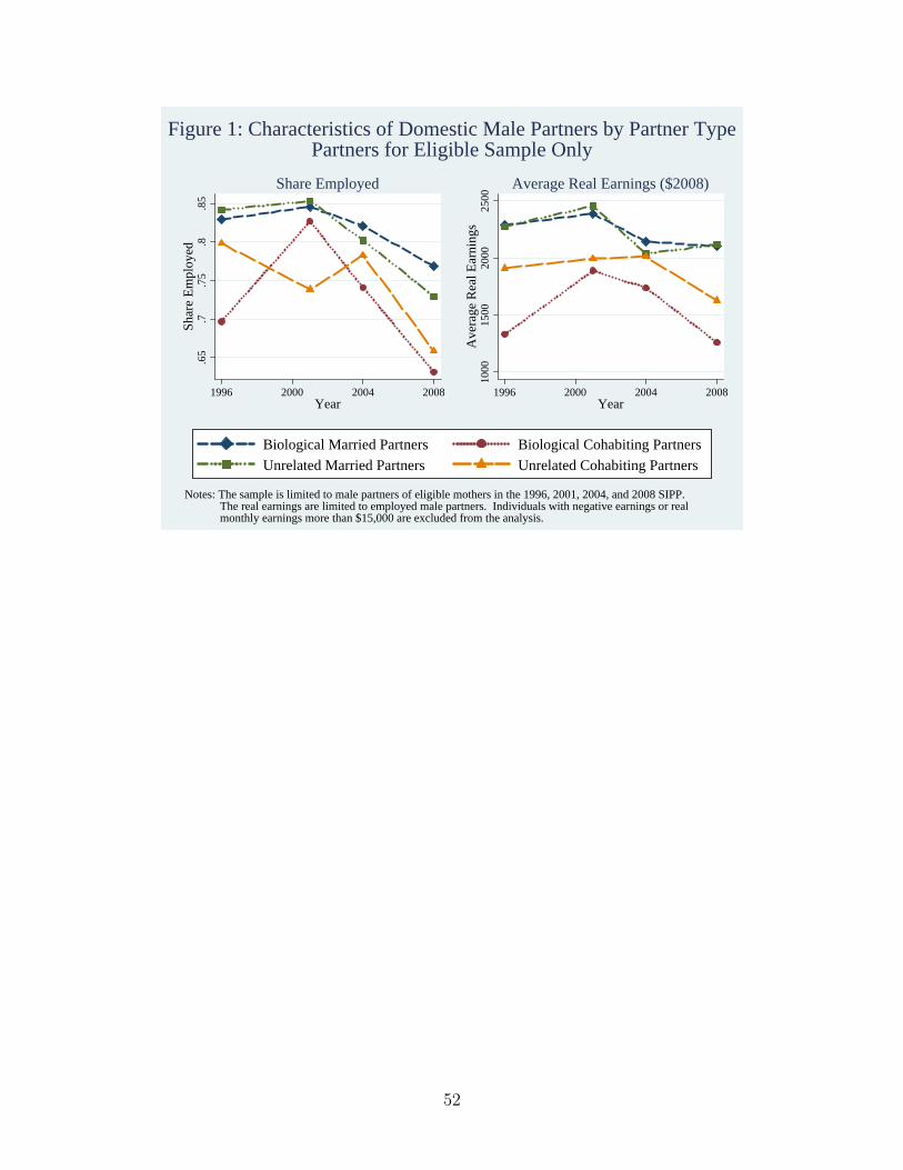
.65

.7.7

5.8

.85

Sha

re E

mpl

oyed

1996 2000 2004 2008Year

Share Employed

1000

1500

2000

2500

Ave

rage

Rea

l Ear

ning

s

1996 2000 2004 2008Year

Average Real Earnings ($2008)

Notes: The sample is limited to male partners of eligible mothers in the 1996, 2001, 2004, and 2008 SIPP. The real earnings are limited to employed male partners. Individuals with negative earnings or real monthly earnings more than $15,000 are excluded from the analysis.

Figure 1: Characteristics of Domestic Male Partners by Partner TypePartners for Eligible Sample Only

Biological Married Partners Biological Cohabiting Partners

Unrelated Married Partners Unrelated Cohabiting Partners

52

Appendix

Table A1: Other Variables in the Empirical AnalysisDemographic Variables, Marriage Market Conditions, and other Policy Variables

Eligible IneligibleVariable Name Sample Sample

Individuals-Level VariablesAge 33.0 37.3Less Than High School 0.28 0.07High School Only 0.38 0.24Some College 0.34 0.35College Degree 0.00 0.34African American 0.27 0.09Asian 0.03 0.05Other Race, Non-white 0.03 0.02Hispanic 0.21 0.10Rural Residence 0.20 0.20

State-Level VariablesUnemployment Rate 0.05 0.05Real Minimum Wage $6.25 $6.28Average Weekly Real Manufacturing Wage $985 $987Monthly Maximum Welfare Benefit $407 $411Percent of Poverty Level: Medicaid Coverage 192% 192%Maximum Real Annual EITC Benefit (for Family of 3) $4,786 $4,813

N 13,828 33,900Notes: The eligible and ineligible samples are defined in the notes to Table 1. Alldemographic variables are for the mother. All labor market and policy variables arestate-specific and lagged one year. Medicaid and EITC values include state supplementsin addition to federally mandated levels. Real values are in $2007. All means areweighted using the SIPP sample weights pooled across 1996, 2001, 2004, and 2008. Allmodels also include state and year dummy variables.

53

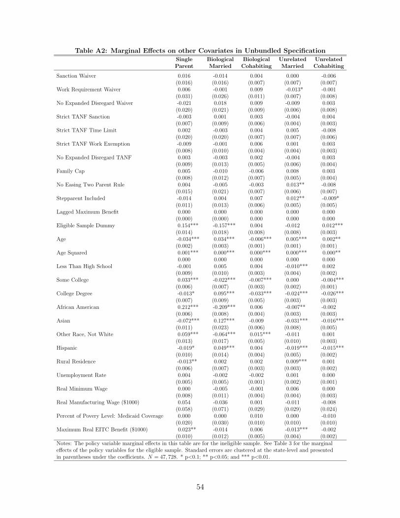
Table A2: Marginal Effects on other Covariates in Unbundled SpecificationSingle Biological Biological Unrelated UnrelatedParent Married Cohabiting Married Cohabiting

Sanction Waiver 0.016 -0.014 0.004 0.000 -0.006(0.016) (0.016) (0.007) (0.007) (0.007)

Work Requirement Waiver 0.006 -0.001 0.009 -0.013* -0.001(0.031) (0.026) (0.011) (0.007) (0.008)

No Expanded Disregard Waiver -0.021 0.018 0.009 -0.009 0.003(0.020) (0.021) (0.009) (0.006) (0.008)

Strict TANF Sanction -0.003 0.001 0.003 -0.004 0.004(0.007) (0.009) (0.006) (0.004) (0.003)

Strict TANF Time Limit 0.002 -0.003 0.004 0.005 -0.008(0.020) (0.020) (0.007) (0.007) (0.006)

Strict TANF Work Exemption -0.009 -0.001 0.006 0.001 0.003(0.008) (0.010) (0.004) (0.004) (0.003)

No Expanded Disregard TANF 0.003 -0.003 0.002 -0.004 0.003(0.009) (0.013) (0.005) (0.006) (0.004)

Family Cap 0.005 -0.010 -0.006 0.008 0.003(0.008) (0.012) (0.007) (0.005) (0.004)

No Easing Two Parent Rule 0.004 -0.005 -0.003 0.013** -0.008(0.015) (0.021) (0.007) (0.006) (0.007)

Stepparent Included -0.014 0.004 0.007 0.012** -0.009*(0.011) (0.013) (0.006) (0.005) (0.005)

Lagged Maximum Benefit 0.000 0.000 0.000 0.000 0.000(0.000) (0.000) 0.000 0.000 0.000

Eligible Sample Dummy 0.154*** -0.157*** 0.004 -0.012 0.012***(0.014) (0.018) (0.008) (0.008) (0.003)

Age -0.034*** 0.034*** -0.006*** 0.005*** 0.002**(0.002) (0.003) (0.001) (0.001) (0.001)

Age Squared 0.001*** 0.000*** 0.000*** 0.000*** 0.000**0.000 0.000 0.000 0.000 0.000

Less Than High School -0.001 0.005 0.004 -0.010*** 0.002(0.009) (0.010) (0.003) (0.004) (0.002)

Some College 0.033*** -0.022*** -0.007*** 0.000 -0.004***(0.006) (0.007) (0.003) (0.002) (0.001)

College Degree -0.013* 0.095*** -0.033*** -0.024*** -0.026***(0.007) (0.009) (0.005) (0.003) (0.003)

African American 0.212*** -0.209*** 0.006 -0.007** -0.002(0.006) (0.008) (0.004) (0.003) (0.003)

Asian -0.072*** 0.127*** -0.009 -0.031*** -0.016***(0.011) (0.023) (0.006) (0.008) (0.005)

Other Race, Not White 0.059*** -0.064*** 0.015*** -0.011 0.001(0.013) (0.017) (0.005) (0.010) (0.003)

Hispanic -0.019* 0.049*** 0.004 -0.019*** -0.015***(0.010) (0.014) (0.004) (0.005) (0.002)

Rural Residence -0.013** 0.002 0.002 0.009*** 0.001(0.006) (0.007) (0.003) (0.003) (0.002)

Unemployment Rate 0.004 -0.002 -0.002 0.001 0.000(0.005) (0.005) (0.001) (0.002) (0.001)

Real Minimum Wage 0.000 -0.005 -0.001 0.006 0.000(0.008) (0.011) (0.004) (0.004) (0.003)

Real Manufacturing Wage ($1000) 0.054 -0.036 0.001 -0.011 -0.008(0.058) (0.071) (0.029) (0.029) (0.024)

Percent of Povery Level: Medicaid Coverage 0.000 0.000 0.010 0.000 -0.010(0.020) (0.030) (0.010) (0.010) (0.010)

Maximum Real EITC Benefit ($1000) 0.023** -0.014 0.006 -0.013*** -0.002(0.010) (0.012) (0.005) (0.004) (0.002)

Notes: The policy variable marginal effects in this table are for the ineligible sample. See Table 3 for the marginaleffects of the policy variables for the eligible sample. Standard errors are clustered at the state-level and presentedin parentheses under the coefficients. N = 47, 728. * p<0.1; ** p<0.05; and *** p<0.01.

54

Table A3: Welfare Policies and Welfare ParticipationProbit Marginal Effects

1996-2008 SIPP Samples 1993-2008 SIPP SamplesSpec 1 Spec 2 Spec 3 Spec 1 Spec 2 Spec 3

Work-Related Waiver PoliciesSanction Waiver -0.047 -0.057**

(0.031) (0.023)

Work Requirement Waiver -0.057 -0.021(0.036) (0.032)

No Expanded Disregard Waiver -0.087*** -0.078* -0.049* -0.044(0.034) (0.044) (0.029) (0.036)

Any Work-Related Waiver Policy -0.039 -0.029(0.029) (0.020)

Number of Work-Related Waiver Policies -0.046** -0.039**(0.023) (0.019)

Strict Work-Related TANF PoliciesStrict TANF Sanction -0.027 -0.041*

(0.022) (0.023)

Strict TANF Time Limit -0.046 -0.047(0.040) (0.039)

Strict TANF Work Exemption 0.016 0.012(0.019) (0.021)

No Expanded Disregard TANF -0.008 -0.033(0.021) (0.021)

Any Work-Related Strict TANF Policy -0.054*** -0.060***(0.016) (0.021)

Number of Work-Related Strict TANF Policies -0.018* -0.025**(0.010) (0.011)

Family-Related TANF PoliciesFamily Cap 0.028 0.016

(0.024) (0.021)

No Easing Two Parent Rule -0.001 -0.002(0.027) (0.025)

Stepparent Included -0.016 -0.003(0.030) (0.025)

Any Family-Related Policy 0.007 0.000(0.024) (0.027)

Number of Family-Related Policies 0.005 0.006(0.018) (0.015)

Notes: Probits estimated on eligible sample only (i.e. without ineligibles as a control group). In the “Any” policy specification, webreak out No Expanded Disregard Waiver from the Any Work-Related Waiver policy because this is necessary for identification, i.e.all states implemented a waiver policy as we have defined them. Standard errors are clustered at the state-level and presented inparentheses under the coefficients. N = 13, 828 for 1996-2008 sample. N = 15, 775 for 1993-2008 sample. * p<0.1; ** p<0.05; and*** p<0.01.

55

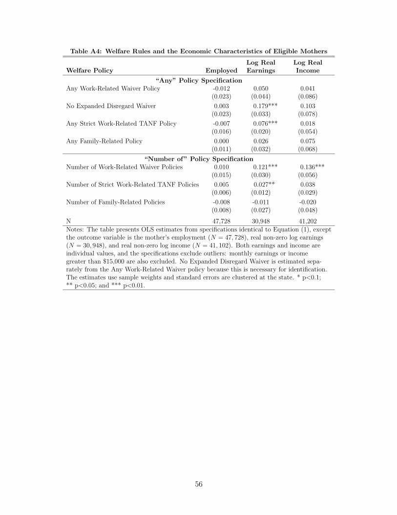
Table A4: Welfare Rules and the Economic Characteristics of Eligible Mothers

Log Real Log RealWelfare Policy Employed Earnings Income

“Any” Policy SpecificationAny Work-Related Waiver Policy -0.012 0.050 0.041

(0.023) (0.044) (0.086)

No Expanded Disregard Waiver 0.003 0.179*** 0.103(0.023) (0.033) (0.078)

Any Strict Work-Related TANF Policy -0.007 0.076*** 0.018(0.016) (0.020) (0.054)

Any Family-Related Policy 0.000 0.026 0.075(0.011) (0.032) (0.068)

“Number of” Policy SpecificationNumber of Work-Related Waiver Policies 0.010 0.121*** 0.136***

(0.015) (0.030) (0.056)

Number of Strict Work-Related TANF Policies 0.005 0.027** 0.038(0.006) (0.012) (0.029)

Number of Family-Related Policies -0.008 -0.011 -0.020(0.008) (0.027) (0.048)

N 47,728 30,948 41,202Notes: The table presents OLS estimates from specifications identical to Equation (1), exceptthe outcome variable is the mother’s employment (N = 47, 728), real non-zero log earnings(N = 30, 948), and real non-zero log income (N = 41, 102). Both earnings and income areindividual values, and the specifications exclude outliers: monthly earnings or incomegreater than $15,000 are also excluded. No Expanded Disregard Waiver is estimated sepa-rately from the Any Work-Related Waiver policy because this is necessary for identification.The estimates use sample weights and standard errors are clustered at the state. * p<0.1;** p<0.05; and *** p<0.01.

56

Table A5: Welfare Policies and Family Structure, Year-by-year Estimates“Any” Policy Specification, Multinomial Logit Marginal Effects

Single Biological Biological Unrelated UnrelatedParent Married Cohabiting Married Cohabiting

Specification using 1996 and 2001 Data

Any Work-Related Waiver Policy -0.016 0.003 0.006 0.005 0.002(0.021) (0.013) (0.005) (0.010) (0.004)

No Expanded Disregard Waiver 0.041** -0.028* -0.004 0.001 -0.011**(0.017) (0.015) (0.009) (0.008) (0.005)

Any Strict Work-Related TANF Policy 0.034** -0.035** -0.002 0.001 0.002(0.014) (0.016) (0.008) (0.009) (0.005)

Any Family-Related Policy 0.013 -0.012 -0.002 -0.005 0.006*(0.015) (0.020) (0.010) (0.011) (0.003)

Specification using 1996 and 2004 Data

Any Work-Related Waiver Policy -0.010 -0.010 0.009* 0.010 0.001(0.018) (0.013) (0.005) (0.009) (0.005)

No Expanded Disregard Waiver 0.063*** -0.060*** -0.001 0.006 -0.009*(0.015) (0.012) (0.007) (0.007) (0.005)

Any Strict Work-Related TANF Policy 0.043*** -0.045*** 0.000 0.005 -0.003(0.016) (0.015) (0.006) (0.008) (0.005)

Any Family-Related Policy -0.025* -0.009 0.006 0.023*** 0.006(0.015) (0.015) (0.006) (0.008) (0.004)

Specification using 1996 and 2008 Data

Any Work-Related Waiver Policy 0.011 -0.026 0.012* -0.001 0.004(0.020) (0.020) (0.007) (0.007) (0.005)

No Expanded Disregard Waiver 0.078*** -0.075*** 0.004 0.004 -0.011*(0.030) (0.026) (0.008) (0.008) (0.006)

Any Strict Work-Related TANF Policy 0.045 -0.069** 0.007 0.016 0.000(0.029) (0.028) (0.008) (0.010) (0.005)

Any Family-Related Policy 0.002 -0.018 -0.002 0.010 0.008**(0.021) (0.022) (0.009) (0.010) (0.003)

Notes: We break out No Expanded Disregard Waiver from Any Work-Related Waiver Policy because this isnecessary for identification, i.e. all states implemented a waiver policy as we have defined them. The marginaleffects for the other control variables for the full 1996-2008 sample from the unbundled specification are shownin Appendix Table A2. Standard errors are clustered at the state-level and presented in parentheses under thecoefficients. N = 22, 123 for 1996/2001 sample. N = 26, 006 for 1996/2004 sample. N = 24, 503 for 1996/2008sample. * p<0.1; ** p<0.05; and *** p<0.01.

57

Table A6: Robustness Tests for the “Any” Specification ResultsMultinomial Logit Marginal Effects

Single Biological Biological Unrelated UnrelatedParent Married Cohabiting Married Cohabiting

II: Standard Difference-in-Differences (as opposed to DDD)Any Work-Related Waiver Policy 0.026 -0.024 0.008 -0.006 -0.003

(0.036) (0.035) (0.011) (0.009) (0.011)No Expanded Disregard Waiver 0.029 -0.034 0.022 -0.019 0.002

(0.048) (0.036) (0.018) (0.013) (0.018)Any Strict Work-Related TANF Policy -0.007 -0.030* 0.031*** 0.004 0.002

(0.018) (0.015) (0.011) (0.009) (0.005)Any Family-Related Policy 0.007 0.007 -0.023* -0.002 0.011*

(0.018) (0.022) (0.014) (0.005) (0.006)

III: Expand “Eligible” Group by removing car ownership restrictionAny Work-Related Waiver Policy -0.003 -0.023* 0.014* 0.007 0.005

(0.017) (0.013) (0.008) (0.006) (0.004)No Expanded Disregard Waiver 0.058*** -0.068*** 0.018*** 0.006 -0.015***

(0.013) (0.013) (0.007) (0.005) (0.005)Any Strict Work-Related TANF Policy 0.041*** -0.059*** 0.011** 0.012*** -0.006

(0.010) (0.010) (0.005) (0.004) (0.004)Any Family-Related Policy -0.012 0.002 0.004 0.002 0.004*

(0.011) (0.014) (0.005) (0.004) (0.002)

IV: Drop College Graduates from “Ineligible” SampleAny Work-Related Waiver Policy -0.011 -0.007 0.009 0.008 0.002

(0.020) (0.013) (0.007) (0.010) (0.006)No Expanded Disregard Waiver 0.061*** -0.049*** 0.001 0.004 -0.016***

(0.015) (0.013) (0.009) (0.009) (0.005)Any Strict Work-Related TANF Policy 0.033*** -0.038*** 0.000 0.006 -0.002

(0.011) (0.009) (0.005) (0.007) (0.003)Any Family-Related Policy 0.010 -0.023 0.000 0.005 0.008***

(0.012) (0.014) (0.008) (0.009) (0.003)

V: Include State-Specific Time TrendsAny Work-Related Waiver Policy -0.005 -0.012 0.010 0.005 0.002

(0.018) (0.011) (0.006) (0.007) (0.005)No Expanded Disregard Waiver 0.058*** -0.053*** 0.001 0.006 -0.013***

(0.013) (0.013) (0.007) (0.007) (0.004)Any Strict Work-Related TANF Policy 0.039*** -0.049*** 0.002 0.010 -0.002

(0.009) (0.009) (0.004) (0.006) (0.002)Any Family-Related Policy 0.006 -0.016 -0.001 0.004 0.008***

(0.011) (0.013) (0.006) (0.007) (0.002)

VI: Include Blended Households in Unrelated HouseholdsAny Work-Related Waiver Policy -0.005 -0.005 0.008 -0.003 0.004

(0.018) (0.015) (0.006) (0.008) (0.005)No Expanded Disregard Waiver 0.057*** -0.059*** 0.007 0.014 -0.019***

(0.013) (0.016) (0.006) (0.011) (0.004)Any Strict Work-Related TANF Policy 0.039*** -0.044*** 0.005 0.005 -0.005**

(0.009) (0.010) (0.004) (0.007) (0.002)Any Family-Related Policy 0.006 -0.011 0.000 -0.002 0.007***

(0.011) (0.015) (0.004) (0.007) (0.003)

VII: Limit Sample to White/Non-Hispanic MothersAny Work-Related Waiver Policy 0.007 -0.007 0.013* -0.010 -0.003

(0.019) (0.017) (0.008) (0.011) (0.007)No Expanded Disregard Waiver 0.002 0.003 0.008 0.001 -0.014***

(0.020) (0.017) (0.008) (0.008) (0.005)Any Strict Work-Related TANF Policy 0.011 -0.013 0.008 -0.002 -0.004

(0.019) (0.016) (0.006) (0.008) (0.004)Any Family-Related Policy 0.016 -0.042** -0.002 0.018* 0.010***

(0.011) (0.019) (0.004) (0.010) (0.003)

Notes: We break out No Expanded Disregard Waiver from Any Work-Related Waiver Policy because this isnecessary for identification, i.e. all states implemented a waiver policy as we have defined them. Standarderrors are clustered at the state-level and presented in parentheses under the coefficients. N = 47, 728for all specifications, with the following exceptions: the traditional difference-in-differences, which onlyuses the eligible sample (N = 13, 828), the estimates that drop college-educated mothers from the ineligiblesample (N = 36, 285), and estimates on the white, non-hispanic sample (N = 30, 730). * p<0.1; ** p<0.05;and *** p<0.01.

58