Welfare measures: CS, CV, EV and PS (Course Micro-economics) Ch 14 Varian Teachers: Jongeneel/Van...
46
Welfare measures: CS, CV, EV and PS (Course Micro-economics) Ch 14 Varian Teachers: Jongeneel/Van Mouche
-
date post
21-Dec-2015 -
Category
Documents
-
view
223 -
download
0
Transcript of Welfare measures: CS, CV, EV and PS (Course Micro-economics) Ch 14 Varian Teachers: Jongeneel/Van...

Welfare measures: CS, CV, EV and PS
(Course Micro-economics)
Ch 14 Varian
Teachers: Jongeneel/Van Mouche

Monetary Measures of Gains-to-Trade
You can buy as much gasoline as you wish at €1 per gallon once you enter the gasoline market.
Q: What is the most you would pay to enter the market?

A: You would pay up to the dollar value of the gains-to-trade you would enjoy once in the market.
How can such gains-to-trade be measured?
Monetary Measures of Gains-to-Trade

Three such measures are:Consumer’s SurplusEquivalent Variation, andCompensating Variation.
Only in one special circumstance do these three measures coincide.
Monetary Measures of Gains-to-Trade
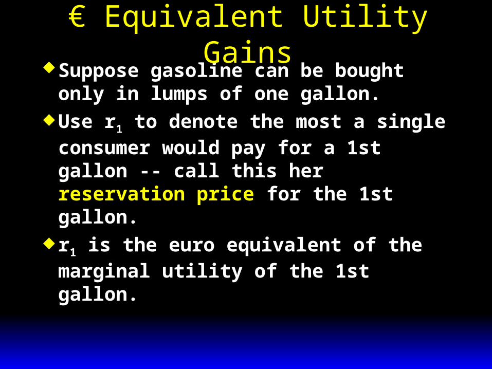
Suppose gasoline can be bought only in lumps of one gallon.
Use r1 to denote the most a single consumer would pay for a 1st gallon -- call this her reservation price for the 1st gallon.
r1 is the euro equivalent of the marginal utility of the 1st gallon.
€ Equivalent Utility Gains
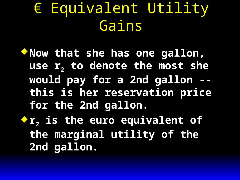
Now that she has one gallon, use r2 to denote the most she would pay for a 2nd gallon -- this is her reservation price for the 2nd gallon.
r2 is the euro equivalent of the marginal utility of the 2nd gallon.
€ Equivalent Utility Gains

Generally, if she already has n-1 gallons of gasoline then rn denotes the most she will pay for an nth gallon.
rn is the euro equivalent of the marginal utility of the nth gallon.
€ Equivalent Utility Gains

r1 + … + rn will therefore be the euro equivalent of the total change to utility from acquiring n gallons of gasoline at a price of €0.
So r1 + … + rn - pGn will be the euro equivalent of the total change to utility from acquiring n gallons of gasoline at a price of €pG each.
€ Equivalent Utility Gains
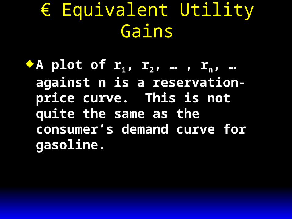
A plot of r1, r2, … , rn, … against n is a reservation-price curve. This is not quite the same as the consumer’s demand curve for gasoline.
€ Equivalent Utility Gains

€ Equivalent Utility GainsReservation Price Curve for Gasoline
0
2
4
6
8
10
Gasoline (gallons)
(€) Res.Values
1 2 3 4 5 6
r1
r2
r3
r4
r5
r6
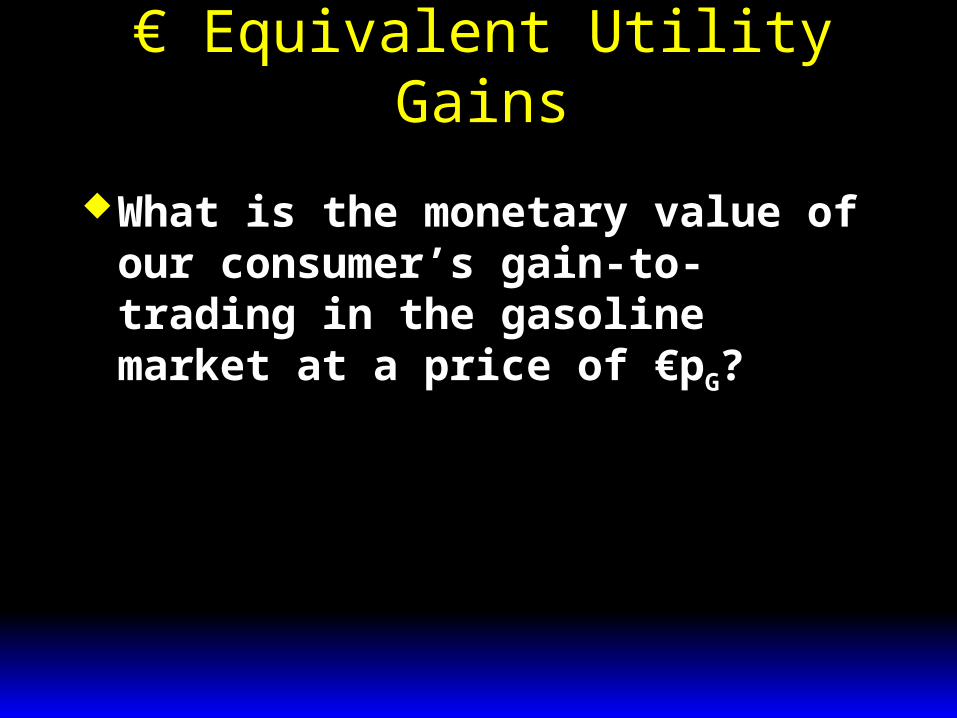
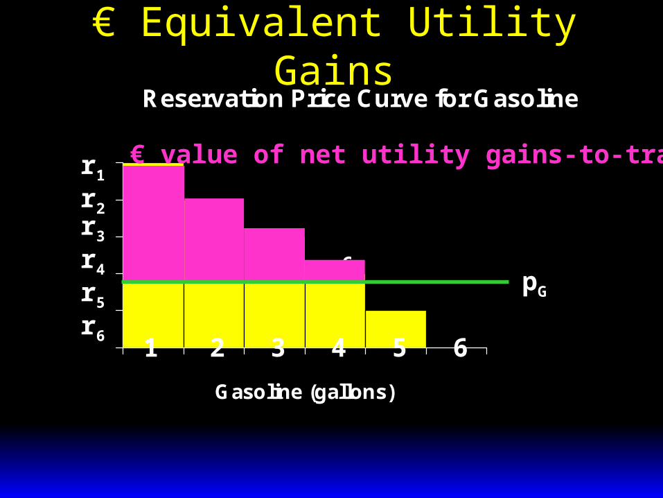
What is the monetary value of our consumer’s gain-to-trading in the gasoline market at a price of €pG?
€ Equivalent Utility Gains
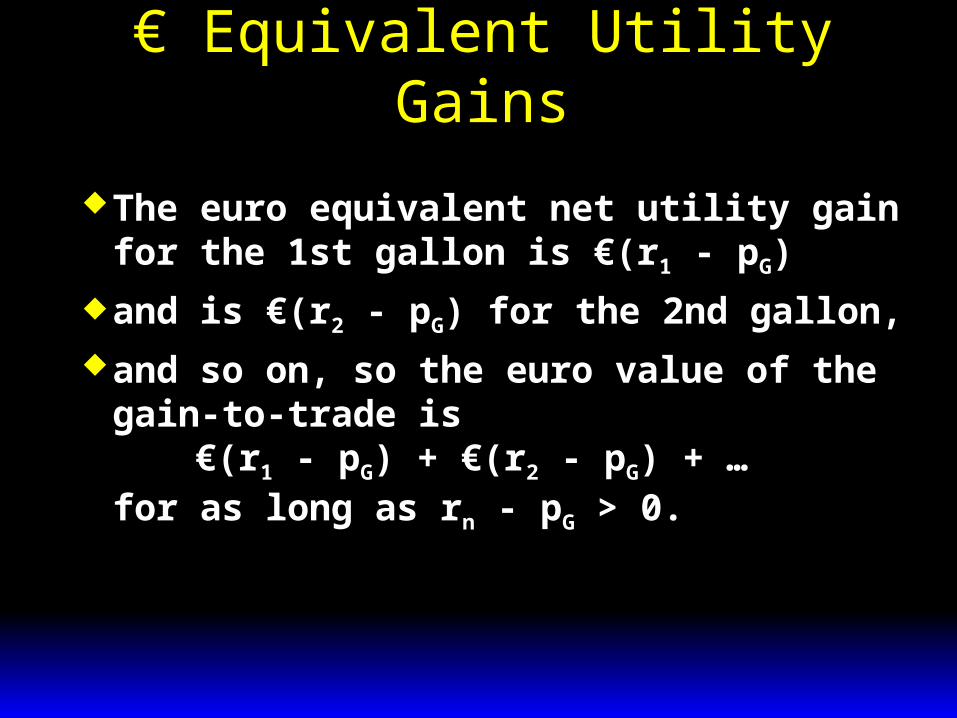
The euro equivalent net utility gain for the 1st gallon is €(r1 - pG)
and is €(r2 - pG) for the 2nd gallon, and so on, so the euro value of the
gain-to-trade is€(r1 - pG) + €(r2 - pG) + …
for as long as rn - pG > 0.
€ Equivalent Utility Gains
€ Equivalent Utility GainsReservation Price Curve for Gasoline
0
2
4
6
8
10
Gasoline (gallons)
€
1 2 3 4 5 6
r1
r2
r3
r4
r5
r6
pG
€ value of net utility gains-to-trade

€ Equivalent Utility Gains
Gasoline
(€) Res.Prices
pG
Reservation Price Curve for Gasoline
€ value of net utility gains-to-trade
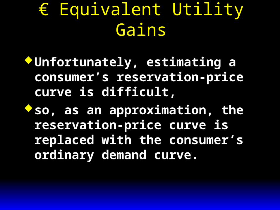
Unfortunately, estimating a consumer’s reservation-price curve is difficult,
so, as an approximation, the reservation-price curve is replaced with the consumer’s ordinary demand curve.
€ Equivalent Utility Gains
A consumer’s reservation-price curve is not quite the same as her ordinary demand curve. Why not?
A reservation-price curve describes sequentially the values of successive single units of a commodity.
An ordinary demand curve describes the most that would be paid for q units of a commodity purchased simultaneously.
Consumer’s Surplus
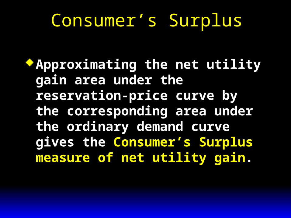
Approximating the net utility gain area under the reservation-price curve by the corresponding area under the ordinary demand curve gives the Consumer’s Surplus measure of net utility gain.
Consumer’s Surplus

Consumer’s Surplus
Gasoline
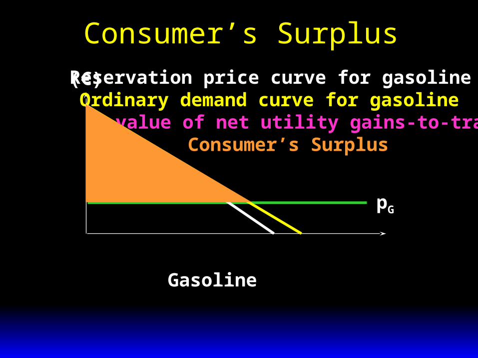
Reservation price curve for gasolineOrdinary demand curve for gasoline
pG
$ value of net utility gains-to-trade
(€)
Consumer’s Surplus
Gasoline
Reservation price curve for gasolineOrdinary demand curve for gasoline
pG
$ value of net utility gains-to-tradeConsumer’s Surplus
(€)
The difference between the consumer’s reservation-price and ordinary demand curves is due to income effects.
But, if the consumer’s utility function is quasilinear in income then there are no income effects and Consumer’s Surplus is an exact € measure of gains-to-trade.
Consumer’s Surplus

Consumer’s Surplus
U x x v x x( , ) ( )1 2 1 2
The consumer’s utility function isquasilinear in x2.
Take p2 = 1. Then the consumer’schoice problem is to maximize
U x x v x x( , ) ( )1 2 1 2 subject to
p x x m1 1 2 .
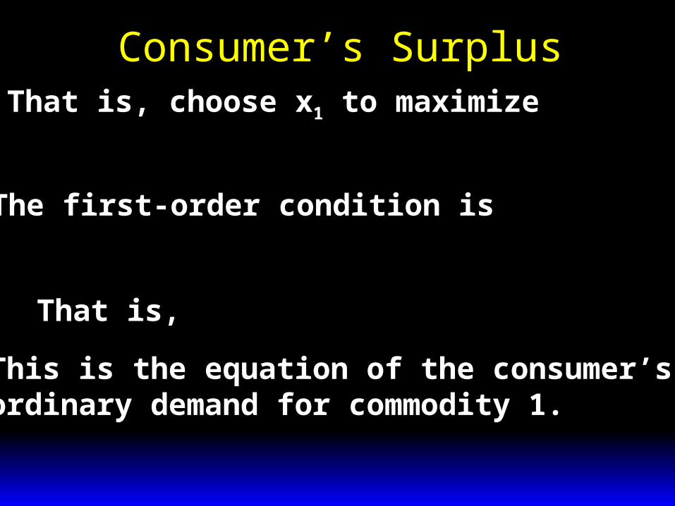
Consumer’s SurplusThat is, choose x1 to maximize
v x m p x( ) .1 1 1 The first-order condition is
v x p'( )1 1 0
That is, p v x1 1 '( ).
This is the equation of the consumer’sordinary demand for commodity 1.
Consumer’s Surplus
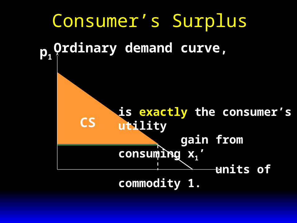
Ordinary demand curve,p1p v x1 1 '( )
x1*x1
'
p1'
CSis exactly the consumer’s utility gain from consuming x1’ units of commodity 1.
CS v x dx p xx '( ) ' ''
1 1 1 101
v x v p x( ) ( )' ' '1 1 10
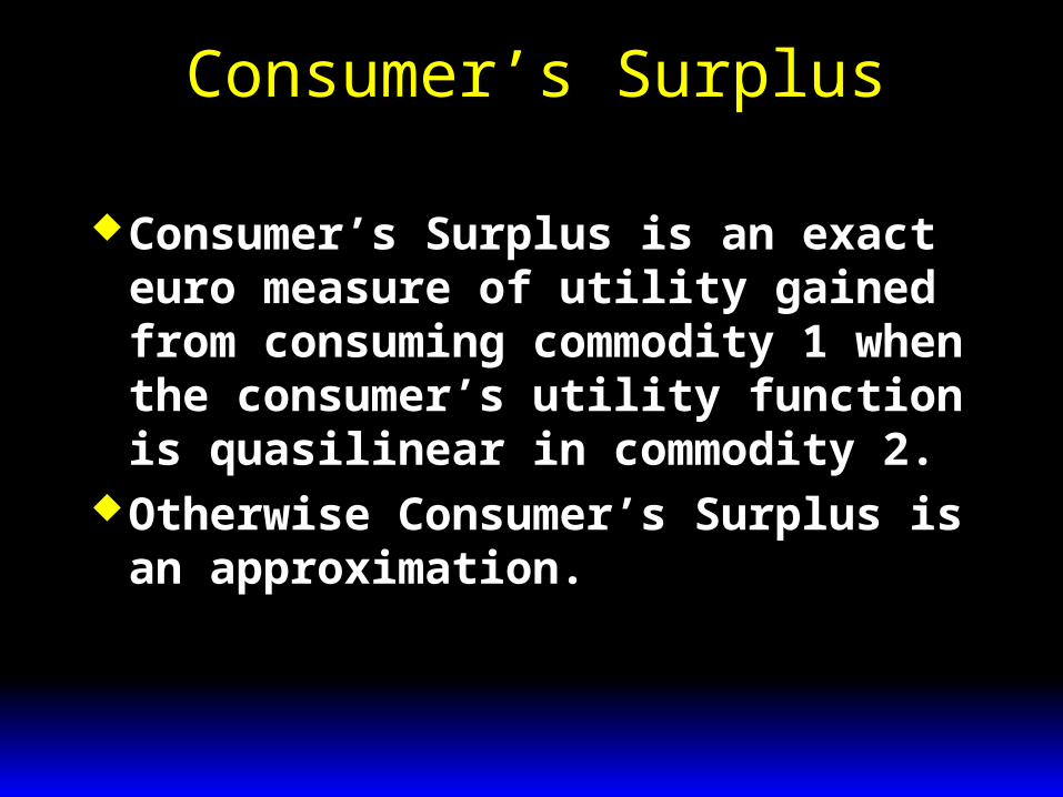
Consumer’s Surplus is an exact euro measure of utility gained from consuming commodity 1 when the consumer’s utility function is quasilinear in commodity 2.
Otherwise Consumer’s Surplus is an approximation.
Consumer’s Surplus
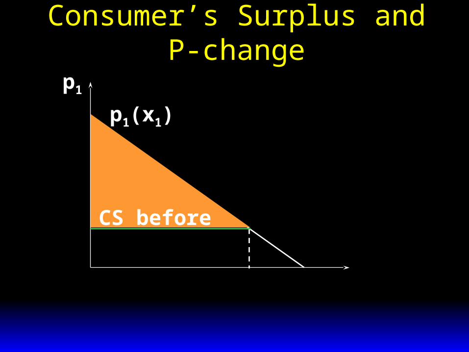
Consumer’s Surplus and P-change
p1
x1*x1
'
CS before
p1(x1)
p1'
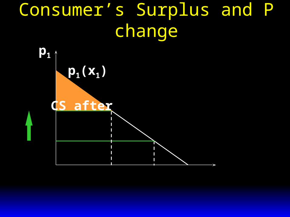
Consumer’s Surplus and P change
p1
x1*x1
'
CS afterp1"
x1"
p1(x1)
p1'
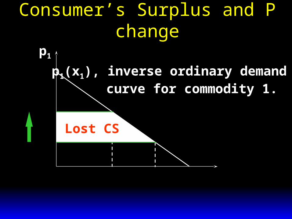
Consumer’s Surplus and P change
p1
x1*x1
'x1"
Lost CS
p1(x1), inverse ordinary demand curve for commodity 1.
p1"
p1'
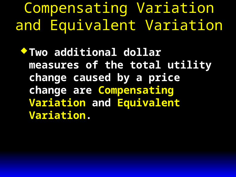
Two additional dollar measures of the total utility change caused by a price change are Compensating Variation and Equivalent Variation.
Compensating Variation and Equivalent Variation

p1 rises.Q: What is the least extra income
that, at the new prices, just restores the consumer’s original utility level?
A: The Compensating Variation.
Compensating Variation
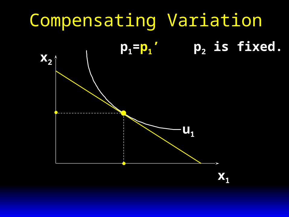
Compensating Variation
x2
x1x1'
u1
x2'
p1=p1’ p2 is fixed.
m p x p x1 1 1 2 2 ' ' '
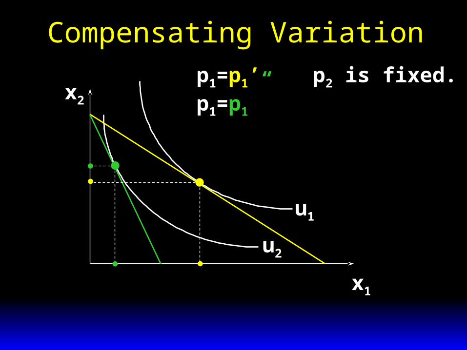
Compensating Variation
x2
x1x1'
x2'
x1"
x2"
u1
u2
p1=p1’p1=p1”
p2 is fixed.
m p x p x1 1 1 2 2 ' ' '
p x p x1 1 2 2" " "
Compensating Variation
x2
x1x1'
u1
u2
x1"
x2"
x2'
x2'"
x1'"
p1=p1’p1=p1”
p2 is fixed.
m p x p x1 1 1 2 2 ' ' '
p x p x1 1 2 2" " "
'"22
'"1
"12 xpxpm

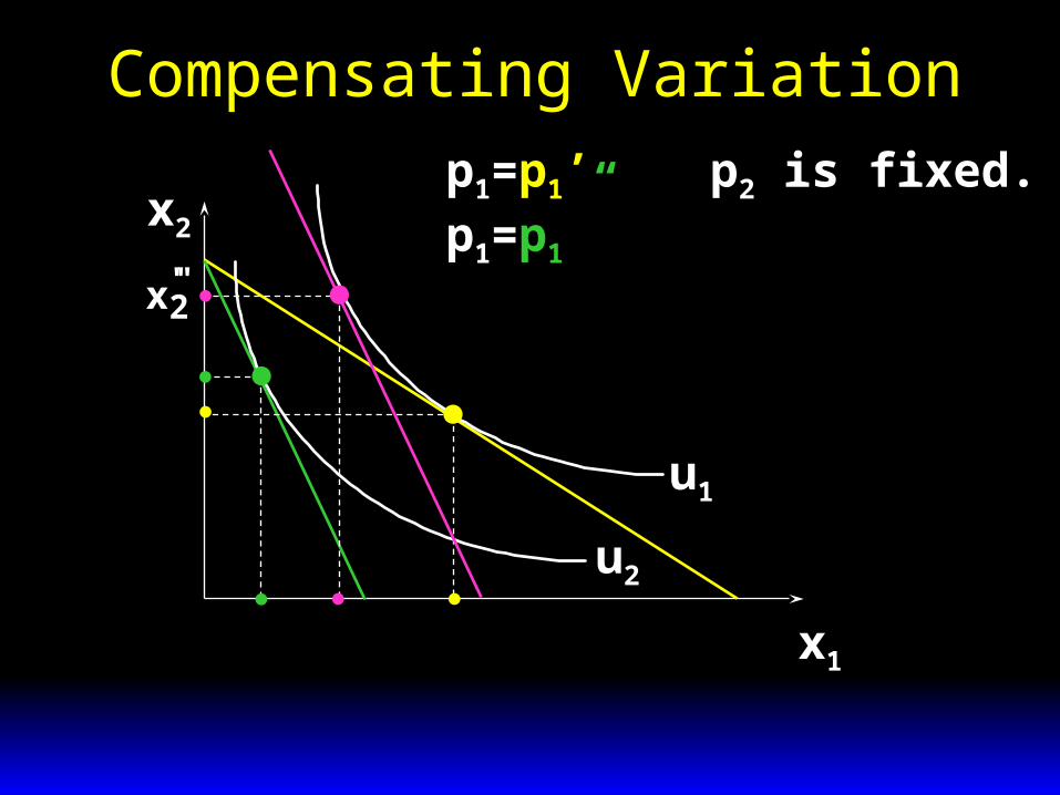
Compensating Variation
x2
x1x1'
u1
u2
x1"
x2"
x2'
x2'"
x1'"
p1=p1’p1=p1”
p2 is fixed.
m p x p x1 1 1 2 2 ' ' '
p x p x1 1 2 2" " "
'"22
'"1
"12 xpxpm
CV = m2 - m1.
p1 rises.Q: What is the least extra income
that, at the original prices, just restores the consumer’s original utility level?
A: The Equivalent Variation.
Equivalent Variation

Equivalent Variation
x2
x1x1'
u1
x2'
p1=p1’ p2 is fixed.
m p x p x1 1 1 2 2 ' ' '
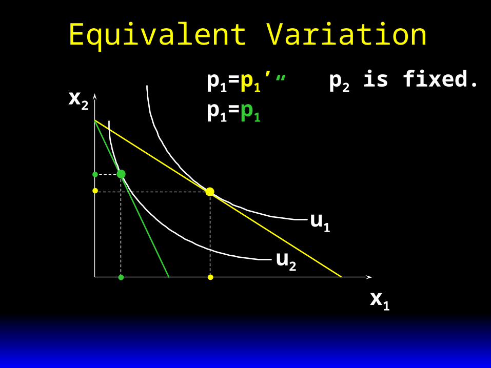
Equivalent Variation
x2
x1x1'
x2'
x1"
x2"
u1
u2
p1=p1’p1=p1”
p2 is fixed.
m p x p x1 1 1 2 2 ' ' '
p x p x1 1 2 2" " "
Equivalent Variation
x2
x1x1'
u1
u2
x1"
x2"
x2'
x2'"
x1'"
p1=p1’p1=p1”
p2 is fixed.
m p x p x1 1 1 2 2 ' ' '
p x p x1 1 2 2" " "
m p x p x2 1 1 2 2 ' '" '"
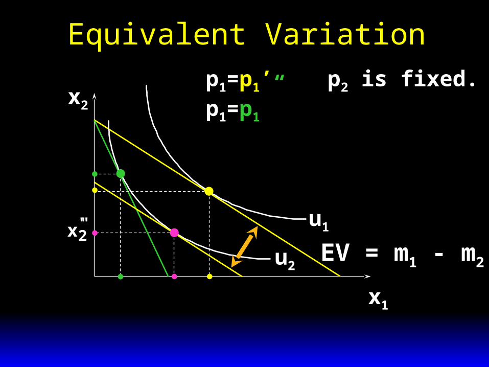
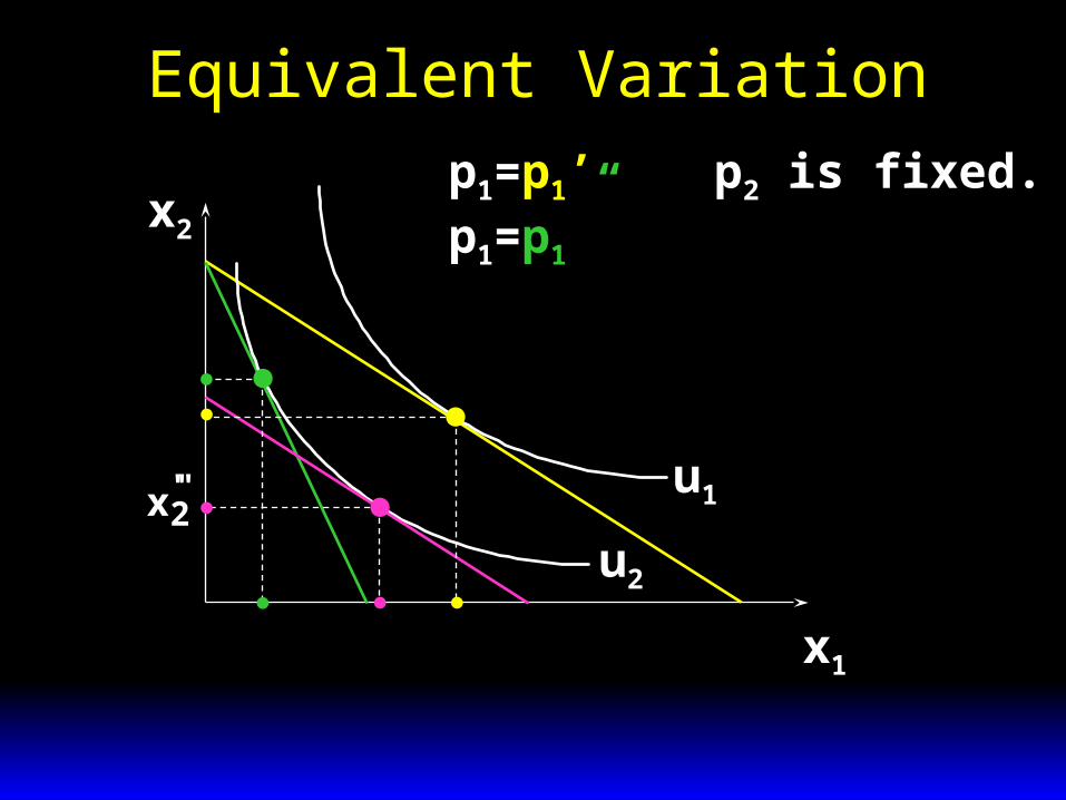
Equivalent Variation
x2
x1x1'
u1
u2
x1"
x2"
x2'
x2'"
x1'"
p1=p1’p1=p1”
p2 is fixed.
m p x p x1 1 1 2 2 ' ' '
p x p x1 1 2 2" " "
m p x p x2 1 1 2 2 ' '" '"
EV = m1 - m2.
Relationship 1: When the consumer’s preferences are quasilinear, all three measures are the same.
Consumer’s Surplus, Compensating Variation and Equivalent Variation
Consumer’s Surplus, Compensating Variation and Equivalent Variation
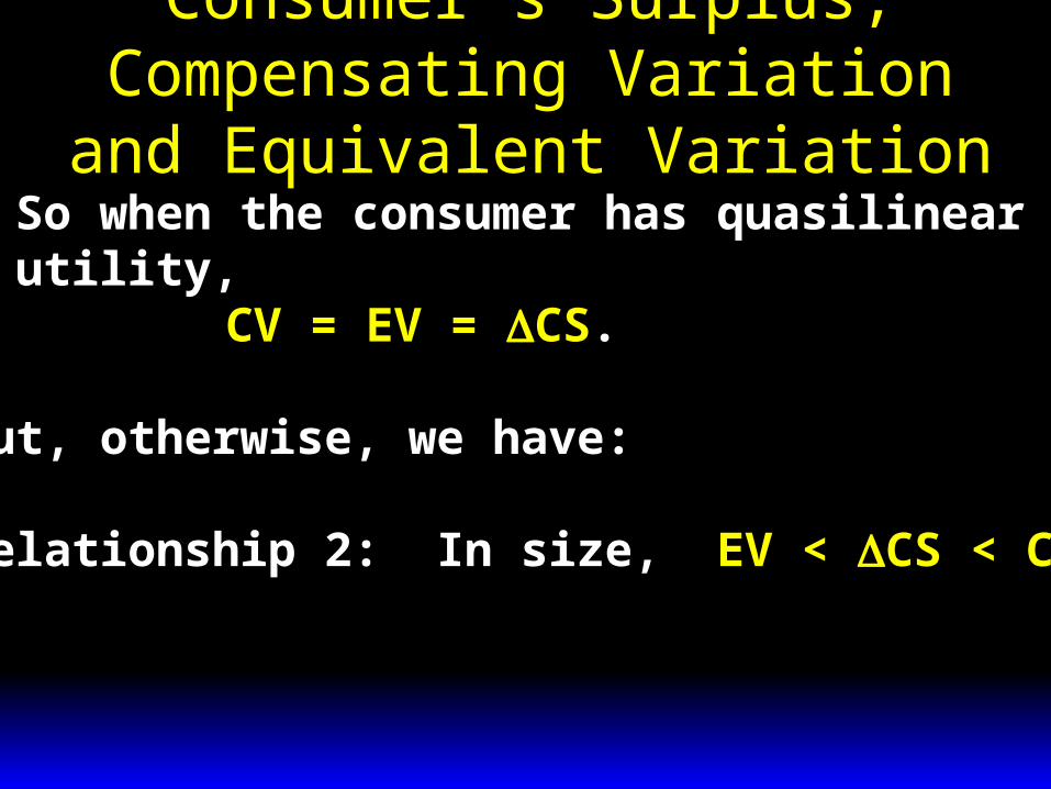
So when the consumer has quasilinearutility,
CV = EV = CS.
But, otherwise, we have:
Relationship 2: In size, EV < CS < CV.
Changes in a firm’s welfare can be measured in dollars much as for a consumer.
Producer’s Surplus
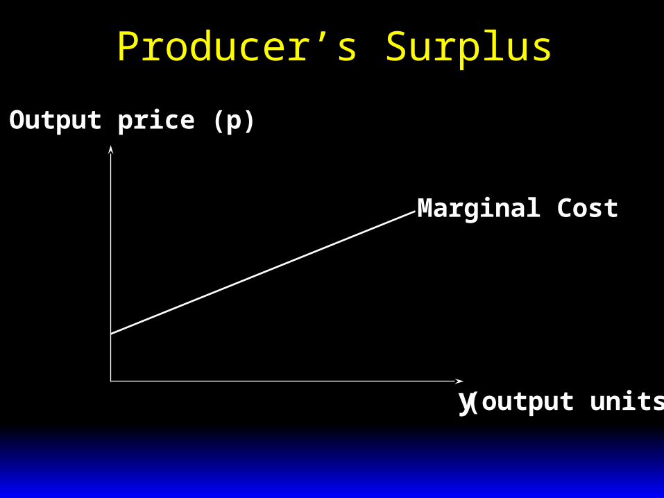
Producer’s Surplus
y (output units)
Output price (p)
Marginal Cost
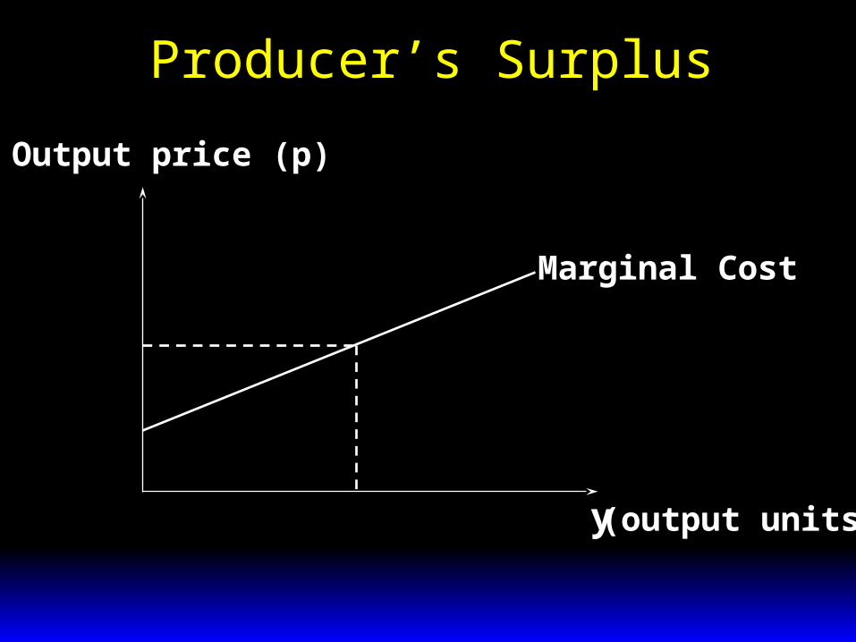
Producer’s Surplus
y (output units)
Output price (p)
Marginal Cost
p'
y'

Producer’s Surplus
y (output units)
Output price (p)
Marginal Cost
p'
y'
Revenue= p y' '
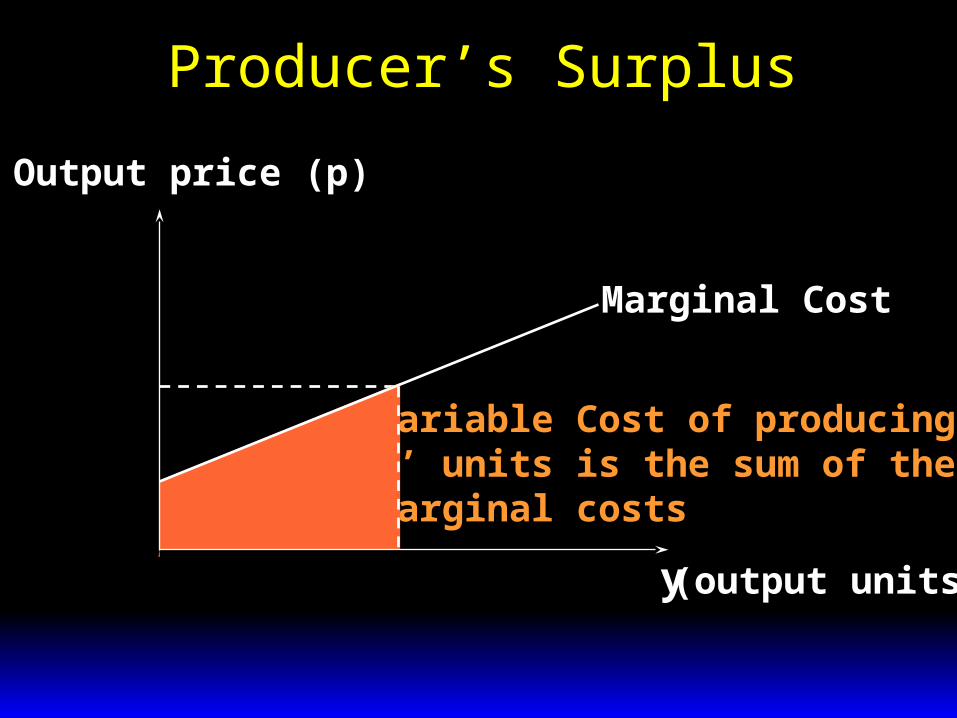
Producer’s Surplus
y (output units)
Output price (p)
Marginal Cost
p'
y'
Variable Cost of producingy’ units is the sum of themarginal costs

Producer’s Surplus
y (output units)
Output price (p)
Marginal Cost
p'
y'
Variable Cost of producingy’ units is the sum of themarginal costs
Revenue less VCis the Producer’sSurplus.