Welfare and Outputwith Income Effects and Taste Shocks

David R. Baqaee

UCLA

Ariel Burstein∗

UCLA

August 2021

Abstract

We characterize how welfare responds to changes in budget sets and technologies when

preferences are non-homothetic or subject to shocks, in both partial and general equi-

librium. We generalize Hulten’s theorem, the basis for constructing aggregate quan-

tity indices, to this context. We show that calculating the response of welfare to a

shock only requires knowledge of expenditure shares and elasticities of substitution

and (given these elasticities) not of income elasticities and taste shocks. We also char-

acterize the gap between welfare and chain-weighted indices. We apply our results to

long- and short-run phenomena. In the long-run, we show that if structural transfor-

mation is caused by income effects or changes in tastes, rather than substitution effects,

then Baumol’s cost disease is twice as important for welfare. In the short-run, we show

that standard deflators understate welfare-relevant inflation because product-level de-

mand shocks are positively correlated with price changes. Finally, using the Covid-19

recession we illustrate the differences between partial and general equilibrium notions

of welfare, and show that real consumption and real GDP are unreliable metrics for

measuring welfare or production.

∗We thank Conor Foley and Sihwan Yang for outstanding research assistance. We thank Andy Atkeson,Natalie Bau, Javier Cravino, Pierre Sarte, David Weinstein, and Jon Vogel for helpful comments. We aregrateful to Emmanuel Farhi and Seamus Hogan, both of whom passed away tragically before this paperwas written, for their insights and earlier conversations on these topics. This paper received support fromNSF grant No. 1947611. The conclusions and analysis are our own, calculated in part on data from NielsenConsumer LLC and provided through the NielsenIQ Datasets at the Kilts Center for Marketing Data Centerat The University of Chicago Booth School of Business. NielsenIQ is not responsible for, had no role in, andwas not involved in analyzing and preparing the results reported herein.

1 Introduction

In this paper, we study how a change in the economic environment affects welfare. For ex-ample, how does an individual’s welfare change when her budget constraint changes, orhow does national welfare change when technologies change? Under some strong assump-tions, a chain-weighted index of real consumption, as measured by statistical agencies, an-swers both of these questions.1 Two of these assumptions are stability and homotheticityof preferences. Both assumptions are highly convenient, but highly counterfactual. Homo-theticity requires that the income elasticity of demand equal one for every good. Stabilityrequires that consumers only change spending between goods in response to changes inincomes and relative prices.2

In this paper, we relax both assumptions and characterize changes in welfare, changesin chained-weighted consumption, and the gap between the two in terms of measurablesufficient statistics. Our baseline welfare measure is the equivalent variation at fixed fi-nal preferences, which answers the question: “holding fixed preferences, how much must con-sumers’ initial endowment change to make them indifferent between their choice sets at t0 and t1?”where t can refer to, for example, time or space.

We first study this problem in partial equilibrium, where choice sets are defined in termsof budget sets (prices are exogenous) and the endowment is income. Here, our welfaremeasure answers a microeconomic question, comparing two budget sets for an infinites-imal agent who does not alter market-level prices through her choices. We then studythis problem in general equilibrium, where choice sets are defined in terms of productionpossibility frontiers (technologies are exogenous) and the endowment is a bundle of factorinputs.3 In this case, our welfare measure answers a macroeconomic question comparingtwo technologies for a collection of agents whose collective decisions alter market-level

1To aggregate data on prices and quantities over multiple goods, chain-weighted indices use good-specificweights that are updated every period. As compared to fixed-weight indices, chain-weighted indices accountfor substitution by consumers. The continuous time analog to a chain-weighted index is called a Divisiaindex. Chained-weighted indices are used to calculate most measures of real economic activity and pricedeflators, ranging from aggregates like output (real GDP), total factor productivity, private consumption andinvestment, to less aggregated objects like industry-level measures of production and inflation. The fact thatunder suitable assumptions these indices approximately measure changes in welfare and production justifiestheir recommended use in the United Nations’ System of National Accounts (see e.g. Chapters 15 and 17 inIMF, 2004).

2As we discuss in detail in Section 2, preference instability is driven by any factor that changes preferencerankings over bundles of goods at fixed prices and income, e.g. aging, illness, advertising, and fads. In theliterature, preference instability and non-homotheticities are typically studied independently. We analyzethem jointly in this paper because both generate the same type of biases in chain-weighted measures of realconsumption. Our results are relevant when either of these forces is active.

3For the macro problem, we consider neoclassical economies with representative (or homogeneous)agents. We show how to generalize all of our results to economies with heterogeneous agents in a com-panion paper, Baqaee and Burstein (2021).

1

prices. When preferences are homothetic and stable, the change in macro and microeco-nomic welfare are both equal to changes in chain-weighted real consumption. However,when preferences are non-homothetic or unstable, the change in macro and micro welfarecaused by the same primitive shock are not equal to each other and neither of them ismeasured by chain-weighted real consumption. Intuitively, macro and micro welfare dif-fer in general because some points on a budget constraint, which may be feasible for anindividual agent, are not feasible for society as a whole due to curvature in the productionpossibility frontier.

We provide exact and approximate characterizations of the change in micro and macrowelfare, and generalize chain-weighted (or more precisely Divisia) indices to measure both.In particular, we extend Hulten (1978) to environments with non-homotheticities and tasteshocks. In contrast to a chain-weighted consumption index, which weighs changes inprices or technologies using observed expenditure shares, welfare-relevant indices weighchanges in prices or technologies using counterfactual expenditure shares calculated un-der the final indifference curve. We show that for this reason, compared to welfare, chain-weighted consumption undercounts expenditure-switching due to income effects or tasteshocks (but not substitution effects).

To understand why, consider the following example. Over the post-war period, spend-ing on healthcare grew relative to manufacturing. Suppose this was caused by consumersgetting older and richer, and the fact that older and richer consumers spend more onhealthcare. If this were the case, then a chain-weighted consumption index would not cor-rectly account for expenditure-switching by consumers. Intuitively, when we compare thepast to the present, we must use demand curves that are relevant for the older and richerconsumers of today, and not demand curves that were relevant in the past. Whereas achained deflator weighs changes in prices that happened during the 1950’s using demandfrom the 1950’s, a welfare-relevant index uses demand from today to weigh changes inprices throughout the sample. We show that a chain-weighted consumption index differsfrom a welfare-relevant index if income- or taste-driven expenditure-switching is corre-lated with changes in relative prices.

Our results for welfare and the gap between welfare and real consumption are ex-pressed in terms of measurable sufficient statistics. In both partial and general equilib-rium, we show that computing the change in welfare does not require direct knowledge ofthe taste shocks or income elasticities. Instead, what we must know are expenditure sharesand elasticities of substitution at the final allocation. For micro welfare, these are the house-hold’s expenditure shares and elasticities of substitution. For macro welfare, these are theinput-output table and elasticities of substitution in both production and consumption.

2

Our results can be used both for ex-post accounting and ex-ante counterfactuals.For very simple economies with one factor, constant returns to scale, and no interme-

diates, the difference between welfare and chain-weighted consumption is approximatelyhalf the covariance of supply and demand shocks. We generalize this formula to more com-plex economies and show how the details of the production structure, like input-outputlinkages, complementarities in production, and decreasing returns to scale, interact withnon-homotheticities and preference shocks to magnify the gap between welfare and chain-weighted consumption. The discrepancies between welfare and chain-weighted consump-tion that we emphasize do not get “aggregated” away. In fact, the more we disaggregate,the more important these discrepancies are likely to become. In this sense, our results arerelated to the literature studying the macroeconomic implications of production networksand disaggregation (e.g. Gabaix, 2011; Acemoglu et al., 2012; Baqaee and Farhi, 2019b).

We illustrate the relevance of our results for understanding long-run and short-run phe-nomena with three applications.

i. Long-run application: Since Baumol (1967), an enduring stylized fact is that indus-tries with slow productivity growth tend to become larger as a share of the economyover time. This phenomenon, known as Baumol’s cost disease, implies that aggregategrowth is increasingly determined by productivity growth in slow-growth industriessince, over time, the industrial mix of the economy shifts to favor these industries.To be specific, from 1947 to 2014, aggregate TFP in the US grew by 60%. If the USeconomy had kept its original 1947 industrial structure, then aggregate TFP wouldhave grown by 78% instead. We show that if this transformation is caused solely byincome effects and demand instability, then welfare-relevant TFP grew by only 47%instead of 60%. We also find a similar pattern in consumption data.

ii. Short-run application: While our first application focuses on long-run patterns, oursecond application shows that gaps between real consumption and welfare are likelypresent at high frequencies too. Whereas industry-level sales shares are relativelystable over short-horizons, firm or product-level sales shares are not. In a firm-levelspecification of our model, we show that when firms’ demand shocks are corre-lated with their supply shocks, there is a gap between welfare-relevant and mea-sured changes in industry-level output and prices. These biases do not disappear aswe aggregate up to the level of real GDP even if firms and industries are infinitesi-mal. When we work with industry-level (rather than disaggregated firm- or product-level) data, we rule out the existence of these biases by assumption. We quantify thesebiases at the industry level using product-level non-durable consumer goods data be-tween 2004 and 2019. We find that standard price indices, like the Sato-Vartia index

3

and chained-weighted price index, understate the welfare-relevant inflation rate byaround 1 percentage point between 2018 and 2019, and this bias grows to more than4 percentage points over the whole sample.

iii. Business-cycle application: Our final application draws on the Covid-19 recession toillustrate the difference between macroeconomic and microeconomic notions of wel-fare. During this recession, household expenditures switched to favor certain sectorsat the same time that those sectors experienced higher inflation. We show that thisimplies that microeconomic welfare, taking changes in prices as given, fell by morethan macroeconomic welfare, taking into account the fact that changes in prices arethemselves caused by demand shocks. Furthermore, real consumption failed to mea-sure either object. This is because in episodes where spending patterns are partlydriven by taste shocks, as in the Covid-19 recession, changes in real consumptiongenerically depend on irrelevant details like the order in which supply and demandshocks hit the economy. In these circumstances, the change in real consumption be-tween two time periods is not a function of only prices and quantities in those twoperiods. Real consumption can be different between the initial and final periods evenif initial and final prices and quantities are the same. The same logic applies to realGDP, which means that real GDP or TFP are unreliable metrics for measuring changesin productive capacity.

Of course, there are other reasons, besides instability and non-homotheticity of prefer-ences, why chained indices fail to accurately measure welfare. Many of these well-knownreasons can be thought of as being due to missing prices and quantities. For example, it iswell-known that real consumption fails to properly account for the creation and destruc-tion of goods if we cannot measure the quantity of goods continuously as their price fallsfrom or goes to their choke price (Hicks, 1940; Feenstra, 1994; Hausman, 1996; Aghion et al.,2019); real consumption does not properly account for changes in the quality of goods (seeSyverson, 2017); and, real consumption fails to properly account for changes in non-marketcomponents of welfare, like changes in the user-cost of durable consumption or leisure andmortality (see Jones and Klenow, 2016). In all of these cases, the problem is that some ofthe relevant prices or quantities in the consumption bundle are missing or mismeasured,and correcting the index involves imputing a value for these missing prices or quantities.The biases caused by non-homotheticities and taste shocks are different in the sense thatthey are not caused by mismeasurement of market prices. For this reason, we abstractfrom these important mismeasurement issues and assume that prices and quantities havebeen correctly measured. If prices and quantities are mismeasured or missing, then our re-sults would apply to the quality-adjusted, corrected, version of prices instead of observed

4

prices. That is, the corrections we derive are different to the ones that are equivalent toadjustments in prices.

Relatedly, taste shocks and mismeasured prices (i.e. unobserved quality change) aresometimes viewed as alternative means to the same end. This is because they can both beused to justify why demand curves shift, even holding prices and incomes fixed. How-ever, while they have similar implications for changes in observed prices and quantities,they have very different implications for welfare. When there are unobserved changes inquality, the gap between welfare and real consumption is caused by a difference betweenmeasured and welfare-relevant prices. In the case of taste shocks (or non-homotheticities),the gap between welfare and real consumption is caused by a difference between measuredand welfare-relevant expenditure shares.

Other related literature. Measuring changes in welfare using a money metric when thereare income effects is standard in microeconomic theory (see, e.g. chapter 7 in Deaton andMuellbauer, 1980).4 We characterize the gap between this notion of welfare and real con-sumption with non-homotheticities and taste shocks. We then extend this to a general equi-librium context, and develop welfare-relevant growth accounting. A standard assumptionin growth accounting is the existence of a stable and homothetic final aggregator. We gen-eralize welfare-relevant growth-accounting to environments where preferences are neitherhomothetic nor stable, and provide exact and approximate characterizations of how wel-fare responds to shocks in general equilibrium (extending Domar 1961, and Hulten 1978).This is an issue of central importance in the literature on disaggregated and productionnetwork models (see, for example, Carvalho and Tahbaz-Salehi, 2018 and the referencestherein).5

A recent and related paper is Redding and Weinstein (2020), who show that variationsin sales are difficult to explain via shifts in supply curves alone, and shifts in demandcurves (i.e. taste shocks) are an important source of variation in the data. Their approachto evaluate welfare changes in the presence of taste shocks contrasts with ours because,unlike us, they treat changes in tastes as being equivalent to changes in price. Opera-tionally, this makes the taste shocks behave like quality shocks. They estimate changes intaste/quality necessary to explain variations in product-level data. However, this only de-

4An alternative to the money-metric approach, which we do not pursue, is axiomatic index theory, whichpostulates axioms that an ideal index should satisfy, and then finds functional forms that satisfy those axioms(see Chapter 16 of IMF, 2004).

5The biases we identify, and the failure of Hulten’s theorem, are not caused by inefficiencies (e.g. markups,wedges, taxes). Baqaee and Farhi (2019a) analyze how growth accounting must be adjusted in inefficienteconomies. Whereas incorporating inefficiencies in production does not affect our micro welfare results, howthey interact with demand instability and non-homotheticity in general equilibrium is beyond the scope ofthis paper.

5

termines changes in the relative size of demand shocks across goods, and it does not pindown changes in the overall level of these shocks. Redding and Weinstein (2020) pin downthe overall level of the shocks by assuming that they are mean zero (see Martin, 2020 fora discussion of this assumption). Our approach is different in that we do not compareutils before and after the taste shocks. Instead we compute changes in equivalent variationkeeping preferences constant for the variation, as advocated by Fisher and Shell (1968) andSamuelson and Swamy (1974). This approach does not require any assumptions about theoverall level of the taste shocks in terms of utils. Moreover, as mentioned above, in prac-tical terms the adjustments we derive require the use of counterfactual expenditure sharesand not counterfactual taste-adjusted prices. We compare the two approaches in more detailin Appendix E.6

Our paper is also related to the literature on structural transformation and Baumol’scost disease. As explained by Buera and Kaboski (2009) and Herrendorf et al. (2013), thisliterature advances two microfoundations for structural transformation. The first expla-nation is all about relative prices differences: if demand curves are not unit-price-elastic,then changes in relative prices change expenditure shares (e.g. Ngai and Pissarides, 2007;Acemoglu and Guerrieri, 2008; Buera et al., 2015). The second explanation emphasizesshifts in demand curves caused by income effects— households spend more of their in-come on some goods as they become richer (e.g. Kongsamut et al., 2001; Boppart, 2014;Comin et al., 2015; Alder et al., 2019), or taste shocks— households spend more of theirincome on some goods as they become older (Cravino et al., 2019). Our results suggestthat structural transformation driven by relative price changes has different welfare impli-cations than structural transformation driven by non-homotheticity or taste shocks.7

The structure of the paper is as follows. In Section 2, we set up the microeconomic prob-lem and provide exact and approximate characterizations of the difference between wel-fare and measured real consumption. In Section 3, we set up the macroeconomic general

6Given CES preferences, Martin (2020) estimates using scanner level data large differences in annual pricechanges between price indices based on fixed initial tastes and final tastes. Other papers studying the rela-tionship between conventional index numbers and welfare in the presence of preference instability includeBalk (1989) who discusses various ways one can define changes in the cost of living, Feenstra and Reinsdorf(2007) who show that the Sato-Vartia index is equal to the CES price index evaluated at some intermediatelevel of taste shifters, and Caves et al. (1982) who show that when preferences are homothetic, translog, butunstable, Tornqvist-based indices correspond to a geometric average of welfare changes under initial andfinal preferences. We characterize welfare (in partial and general equilibrium) at either initial or final prefer-ences and using either EV or CV. In contrast to Tornqvist and Sato-Vartia, studied by Caves et al. (1982) andFeenstra and Reinsdorf (2007), Divisia indices cannot generically be interpreted as corresponding to any mix-ture of well-defined preferences. This is because, as we discuss in Section 5, Divisia (or chained) indices arepath-dependent, so they can violate basic properties like assigning a higher value to a strictly larger budgetset.

7For welfare analysis with non-homothetic preferences in other contexts such as cross-country real incomecomparisons and gains from trade, see Feenstra et al. (2009) and Fajgelbaum and Khandelwal (2016).

6

equilibrium model and provide exact and approximate characterizations of the differencebetween welfare and measured real output changes. Whereas in Section 3 we present ourmacro results in terms of endogenous sufficient statistics, in Section 4 we solve for theseendogenous sufficient statistics in terms of microeconomic primitives and consider somesimple but instructive analytical examples. Our applications are in Section 5. We discusssome extensions in Section 6 and conclude in Section 7. Proofs are in the appendix.

2 Microeconomic Changes in Welfare and Consumption

In this section, we consider changes in budget constraints in partial equilibrium. We askhow consumers value these changes, and compare these measures of welfare with mea-sures of real consumption. This section helps build intuition for Section 3, where we modelthe equilibrium determination of prices.

2.1 Definition of Welfare and Real Consumption

In this subsection we define welfare and real consumption. Measuring changes in welfareusing equivalent variation is standard when preferences are stable. However, measuringwelfare changes in the presence of unstable preferences is less common and therefore wediscuss this issue in some detail.

Consider a set of preference relations, x, over bundles of goods c ∈ RN, where N isthe number of goods. These preferences are indexed by x, which represents anything thataffects preference rankings over bundles of goods. For example, x could be calendar time,age, exposure to advertising, or state of nature. For every x, we represent the preferencerelation x by a utility function u(c; x). Since the consumer makes no choices over x,preferences over x, if they exist, are not revealed by choices. Hence, whereas u(c; x) >

u(c′; x) implies that x prefers c to c′, a comparison of u(c; x′) and u(c; x) is not necessarilymeaningful and may not encode any information.8

There are two properties of preferences that are analytically convenient benchmarksthroughout the rest of the analysis.

Definition 1 (Homotheticity). Preferences over goods c are homothetic if, for every positivescalar a > 0 and every feasible c and x, we can write

u(ac; x) = au(c; x).8In Section 6, we discuss situations in which x is endogenously chosen and valued by the consumer,

such as leisure, but its price and quantity are not being measured. We also discuss situations in which x isendogenously chosen by firms, such as advertising.

7

Definition 2 (Stability). Preferences over goods c are stable if there exists a time-invariantfunction Φ (·) such that the utility function can be written as u(c; x) = U(Φ(c); x) for everyfeasible c and x.

If preferences are stable, x can change over time (e.g. households get higher or lower utilsfrom all goods) but, since x is separable from c, these changes do not impact preferencesover bundles of goods c. If preferences are not stable, we say that they are unstable.

Given preferences encapsulated in u, the indirect utility function of the consumer, forany value of x, is

v(p, I; x) = maxcu(c; x) : p · c = I.

where p is a price vector over goods and I is expenditures (which we interchangeably referto as income). The vector p includes all relevant prices, and if x is intertemporal, then pincludes the path of current and future prices.9

Consider shifts in the budget set as prices and income change from pt0 and It0 to pt1

and It1 . Here, t0 and t1 simply index the vector of prices and income being compared.Motivated by our applications, we refer to this index as time, but it could equally refer tospace. This change in the budget set is accompanied by changes in x from xt0 to xt1 .

Since utility is only defined up to monotone transformations, changes in utility do nothave meaningful units. When prices are exogenous, we measure changes in utility usingcorresponding changes in income. Our baseline measure of microeconomic welfare is de-fined as follows.

Definition 3 (Micro Welfare). The change in welfare measured using the micro equivalentvariation with final preferences is EVm(pt0 , It0 , pt1 , It1 ; xt1) = φ where φ solves

v(pt1 , It1 ; xt1) = v(pt0 , eφ It0 ; xt1). (1)

In words, EVm is the change in income (in logs), under initial prices pt0 , that a consumerwith preferencesxt1

would need to be indifferent between the budget set defined by initialprices (pt0 , eφ It0) and the new budget set defined by new prices and income (pt1 , It1). Thenew budget set is preferred to the initial one, if and only if, EVm is positive. We focuson xt1

since, for intertemporal comparisons (as opposed to interregional comparisons),today’s preferences are more relevant than the those of the past. Hence, if t1 represents thepresent and t0 represents the past, then xt1

is more relevant than xt0. See Remark 2 and

Appendix C where we show that our methods readily extend to xt0and compensating

(as opposed to equivalent) variation. Finally, the superscript m in EVm represents the factthat this is the micro equivalent variation, since we take prices as given.

9We explicitly discuss how to apply our results in dynamic economies in Section 4.3.

8

Discussion of our welfare criterion. Following Fisher and Shell (1968), the welfare cri-terion in Definition 3 measures the change in welfare by presenting the consumer with ahypothetical choice holding fixed their preferences. To be concrete, suppose that x repre-sents the age of the consumer. Clearly, we cannot meaningfully compare the amount ofutils an individual derives from watching cartoons as a child to the amount of utils thatindividual derives from drinking coffee as an adult. Since consumers never make choicesabout how old they are, their preferences across consumption goods consumed at differentages are not revealed by their choices. In the words of Heraclitus: “No man ever steps inthe same river twice, for it’s not the same river and he’s not the same man.” However, ifwe fix the consumer’s age x, we can meaningfully compare the consumer’s choices aboutbudget sets they faced at different points in their life or that they may face in the future.

This approach, of holding x constant, is different to the one taken when x representssome form of quality change. Quality adjustments are applicable to situations where theconsumer can conceivably make choices between the good at differing levels of quality.For example, if a box of chocolates undergoes quality change so that each box now containstwice as many chocolates, the consumer can conceivably make choices between the old andnew boxes that reveal how much they value the quality change. Taste changes, on the otherhand, do not involve meaningful choices from the consumer’s perspective. Our approachof holding x constant allows us to study welfare in situations where, either for practical orphilosophical reasons, it is not possible to model preferences over x itself.

Real Consumption. Having defined changes in welfare, we now define changes in realconsumption. The change in real consumption corresponds to what national income ac-countants and statistical agencies do when given data on the evolution of prices p andconsumption bundles c.

Definition 4 (Real consumption). For some path of prices and quantities that unfold as afunction of time t, the change in real consumption from t0 to t1 is defined to be

∆ log Y =∫ t1

t0∑i∈N

bitd log cit

dtdt =

∫ t1

t0∑i∈N

bid log ci, (2)

where bit ≡ pitcit/It is the budget share of good i given prices, income, and preferences attime t.10

The last equation on the right-hand side suppresses dependence on t in the integral. Wesometimes use this convention to simplify notation. Equation (2) is called a Divisia quantity

10For any variable z, we denote by dz its change over infinitesimal time intervals, so that ∆z =∫ t1

t0dz.

9

index. In practice, since perfect data is not available in continuous time, statistical agenciesapproximate this integral via a (Riemann) sum using chained indices. We abstract from theimperfections of these discrete time approximations in this paper.11 Moreover, we assumethat the data on prices and quantities is perfect — completely accurate, comprehensive, andadjusted for any necessary quality changes. This is because the important and well-studiedbiases associated with imperfections in the data, like the lack of quality adjustment, missingprices, or infrequent measurement, are different to the biases we study.

Define the expenditure function for any value of x by

e(p, u; x) = minc∑

i∈Npici : u(c; x) = u.

The budget share of good i (given prices p, preferences x, and a level of utility u) is

bi(p, u; x) ≡ pici(p, u; x)e (p, u; x)

=∂ log e(p, u; x)

∂ log pi, (3)

where the second equality is Shephard’s lemma. Using the budget constraint, real con-sumption in (2) can be expressed in terms of changes in nominal income deflated by pricechanges:

∆ log Y = ∆ log I −∫ t1

t0∑i∈N

bi(pt, ut, xt)d log pit

dtdt. (4)

In words, changes in real consumption are equal to changes in income minus changes in theconsumption price deflator. Notice that changes in real consumption (or the consumptionprice deflator) potentially depend on the entire path of prices and quantities between t0

and t1 and not just the initial and final values. This is unlike welfare changes, EVm, whichdepend only on initial and final prices and incomes and not on their entire path.

2.2 Relating Welfare and Consumption

We consider how real consumption and welfare change in response to changes in the bud-get set and the preferences of the consumer. We first consider globally exact results andthen local approximations. The results are stated in terms of changes in prices and income,which we endogenize in Sections 3 and 4.

11In discrete time, one can approximate this Riemann integral in different ways. For example, we can useleft-Rieman sums (Chained Laspeyres), right-Riemann sums (Chained Paasche), or mid-point Riemann sums(Chained Tornqvist or Fisher). In continuous time, all of these procedures are equivalent and yield the sameanswer.

10

Global results. We start by expressing changes in welfare in terms of changes in pricesand expenditure shares.

Lemma 1 (Micro Welfare). For any smooth path of prices, income, and tastes that unfold as afunction of time t, micro welfare changes are given by

EVm = ∆ log I −∫ t1

t0∑i∈N

bi(pt, ut1 , xt1)d log pit

dtdt, (5)

where bi(pt, ut1 , xt1) = bi(pt, v(pt1 , It1 ; xt1); xt1) denotes budget shares at prices pt, but fixing finalpreferences xt1 and final utility ut1 = v(pt1 , It1 ; xt1).

Comparing (5) and (4) clarifies the differences between welfare and real consumption.Real consumption weighs changes in prices at time t by observed budget shares at time t. Incontrast, welfare weighs changes in prices at time t by some hypothetical budget shares (atfixed utility and tastes). Intuitively, EVm depends only on the terminal value of xt1 becausethis is the only value of x that appears in the definition of EVm. Moreover, EVm dependson budget shares evaluated at final utility, ut1 , since EVm adjusts the level of income in t0

to make consumers as well off as they are in t1. For instance, if welfare increases from t0 tot1, consumers must be given more income in t0 to make them indifferent between t0 andt1. As we give consumers more income in t0, the shape of their indifference curve changesuntil it mirrors the one in t1. This means that the shape of the indifference curve relevantfor the comparison is the one at t1.12

Lemma 1 follows from the observation that EVm can be re-expressed, using the expen-diture function, as

EVm = loge (pt0 , v(pt1 , It1 ; xt1); xt1)

e (pt0 , v(pt0 , It0 ; xt1); xt1)= ∆ log I − log

e (pt1 , v(pt1 , It1 ; xt1); xt1)

e (pt0 , v(pt1 , It1 ; xt1); xt1),

and recognizing that the second term can be written as the integral in (5).13

12When there are no taste shocks, real consumption, defined by (2), is a multi-good version of the changein consumer surplus, which is the area under the Marshallian demand curve. Similarly, by equation (5),welfare is the area under a Hicksian demand curve. Hence, in a partial equilibrium context with stablepreferences, the gap between real consumption and welfare is also the gap between consumer surplus andwelfare, studied by Hausman (1981) and McKenzie and Pearce (1982) amongst others. This equivalence doesnot hold when preferences are unstable (since Marshallian consumer surplus is not the same as chained realconsumption) or in general equilibrium (since micro and macro welfare are not the same, as we discuss inSection 4).

13By definition, EVm only depends on initial and final prices and income, given t1 preferences. By thegradient theorem for line integrals, the integral in (5) is path-independent and can be computed under anycontinuously differentiable path of prices that go from pt0 to pt1 . When comparing EVm and real consump-tion, we consider the integral under the realized path of prices over time, which as described in the text isassumed to be available in continuous time.

11

To make the notation more compact, denote the welfare-relevant budget shares in Lemma1 by

bevi (pt) ≡ bi(pt, ut1 , xt1).

We can reinterpret these hypothetical budget shares bev(p) as corresponding to those ofa fictional consumer with homothetic and stable preferences with expenditure functioneev (p, u) = e (p, ut1 ; xt1)

uut1

, where ut1 = v(pt1 , It1 ; xt1). This implies that we can calculatechanges in welfare given changes in prices based on budget shares bev(p), without needingto know income elasticities or the nature of demand shocks. This is because this fictionalconsumer has homothetic and stable preferences, so all income elasticities are equal to oneand there are no demand shocks. To compute bev(p), we need to know the terminal budgetshares and the terminal elasticities of substitution, as discussed in the following remark.

Remark 1 (Non-homothetic CES preferences). To illustrate how Lemma 1 can be used,consider a non-homothetic CES example as in Comin et al. (2015) or Fally (2020). For thisdemand system, the following equation pins down changes in budget shares at time t:

d log bit=[1− θ0] [d log pit −Ebt(d log pt)]︸ ︷︷ ︸substitution effects

+[εit − 1] [d log It −Ebt(d log pt)]︸ ︷︷ ︸income effects

+ d log xit︸ ︷︷ ︸taste shock

, (6)

where Eb(·) is a weighted average using budget shares in place of “probability” weights.The elasticity θ0 is the (constant utility) elasticity of substitution across goods and εit is theincome elasticity of good i. The term d log xit is a demand shifter (i.e. a taste shock), aresidual that captures changes in expenditure shares not attributable to changes in incomeor prices. Note that when εit is equal to 1 for every i and t, final demand is homothetic, andwhen xit is constant for all i and t, final demand is stable.14

If we know bt1 , we can construct the welfare-relevant budget shares bev(p) between t0

and t1 by iterating on

d log bevit = [1− θ0] [d log pit −Ebev

t(d log pt)], (7)

starting at t1 with initial value bevt1

= bt1 and going back to t0. These are changes in budgetshares which are only due to substitution effects, and hence omit the last two terms inequation (6). Given the path of bev

t , we can then apply Lemma 1. For non-homothetic CES,

14Since bit are expenditure shares that always add up to one, it must be that Ebt(d log xt) = 0 and Ebt(εt) =1. See Appendix D for a derivation and mapping between ε and d log x and primitive preference parameters.

12

the integral in Lemma 1 has a closed form solution15

EVm = ∆ log I −∫ t1

t0∑i∈N

bevi (pt)

d log pit

dtdt = ∆ log I + log

(∑

ibit1

(pit0

pit1

)1−θ0) 1

1−θ0

. (8)

This shows that the income elasticities and taste shocks are not directly required.16,17

If bt1 is not known, we first have to predict bt1 by iterating on equation (6) from t0 to t1 toobtain bt1 . This first step requires full knowledge of demand shocks and income elasticitiesover time (see Appendix D for more details). Once in possession of bt1 , apply (8) to get thechange in welfare.

Remark 2 (Compensating Variation under Initial Preferences). Our baseline measure ofwelfare changes is equivalent variation under final preferences. An alternative would beto use compensating variation under initial preferences. Every result in the paper can betranslated into compensating variation under initial preferences simply by reversing theflow of time. In particular, whereas Lemma 1 preserves the shape of the indifference curveat the final allocation, the compensating variation counterpart to Lemma 1 preserves theshape of the indifference curve at the initial allocation. Hence, calculating compensat-ing variation requires knowledge of initial budget shares and elasticities of substitution,whereas equivalent variation requires knowledge of final budget shares and elasticities ofsubstitution. This means that EVm is more convenient for ex-post comparisons and CVm

(at initial preferences) is more convenient for ex-ante comparisons or counterfactuals. Thisis because in these cases, we use “today’s” budget shares and elasticities of substitution toundertake the welfare comparisons (without needing knowledge of taste shocks or incomeelasticities). See Appendix C for more details.18

15In Appendix D.2, we show that when preferences are non-homothetic CES, changes in the utility indexare not the same as changes in equivalent (or compensating) variation. Hence, the non-homothetic CES utilityindex is not a money-metric for welfare.

16In practice, estimating the elasticity of substitution θ0 may require knowing the income elasticities (viaSlutsky’s equation). However, if the expenditure share of each good is sufficiently small, then θ0 can beestimated without knowledge of income elasticities. Auer et al. (2021) estimate the relevant price elasticitiesand apply Lemma 1 to measure the heterogeneous welfare effects of changes in foreign prices in the presenceof demand non-homotheticities.

17The result that only terminal elasticities of substitution are necessary to calculate EVm is true for arbitrarynon-CES functional forms, but since the intuition for the more general case is similar to the CES case, weleave the more general non-parametric results in Appendix I. We use non-homothetic CES in our worked-out examples since it provides a clean separation between substitution elasticities (necessary for computingwelfare) and other parameters of the utility function, in contrast to other commonly used non-homotheticdemand systems such as PIGL and AIDS. Furthermore, substitution elasticities are symmetric and constantfor CES, which also helps keep the examples intuitive.

18In Appendix C we show that, up to a second-order approximation (but not globally), changes in real con-sumption equal a simple average of equivalent variation under final preferences and compensating variationunder initial preferences.

13

We now contrast changes in real consumption and welfare.

Proposition 1 (Consumption vs. Welfare). Given a smooth path of prices, income, and tastesthat unfold as a function of time t, the difference between welfare changes and real consumption is

EVm − ∆ log Y =∫ t1

t0∑i∈N

(bit − bevit )

d log pit

dtdt = (t1 − t0)EtCov (bt − bev

t , d log pt) ,

where the covariance is calculated across goods at a point in time, and the average is calculatedacross time between t0 and t1.

An immediate consequence of Proposition 1 is the well-known result that real consump-tion is equal to changes in equivalent variation if, and only if, preferences are homotheticand stable. This is because when preferences are stable and homothetic, budget sharesdo not depend on x or changes in utility u over time. Hence, whenever preferences arehomothetic and stable, bev

it = bit for every path of shocks and every t.To gain more intuition for the gap between welfare and real consumption, we use a

second-order approximation.

Local results. Consider local approximations of the objects of interest as the time periodgoes to zero, t1 − t0 = ∆t → 0.19 Throughout the rest of the paper, a second-order ap-proximation means that the remainder term is of order ∆t3. We focus on second-order ap-proximations to capture the interaction between price changes and expenditure-switching,which is the source of the gaps between real consumption and welfare changes.

Differentiating (4) twice, and evaluating at t0, implies that the change in real consump-tion around t0 is approximately

∆ log Y ≈ ∆ log I −Eb(∆ log p)︸ ︷︷ ︸first-order

− 12

Covb (∆ log b, ∆ log p)︸ ︷︷ ︸second-order

, (9)

where Eb(·) and Covb(·) are evaluated using budget shares at t0 as probability weights. Thefirst-order term is just the change in nominal income deflated by average prices (where theaverage uses budget shares at the point of linearization). The second-order terms dependon how expenditures change in response to the shock, and these changes in expenditurescan be driven by either substitution effects, income effects, or taste shocks.

19For our local approximations, we assume that the exogenous parameters (prices, income, and tasteshifters) are smooth functions of t and that the expenditure function is a smooth function of x.

14

To make the relationship between real consumption and welfare more concrete, we usethe non-homothetic CES aggregator introduced in Remark 1.20

Proposition 2 (Approximate Micro using Marshallian Demand). Consider some perturbationin demand ∆ log x, prices ∆ log p, and income ∆ log I. Then, to a second-order approximation, thechange in real consumption is

∆ log Y ≈ ∆ log I −Eb (∆ log p)− 12(1− θ0)Varb (∆ log p)︸ ︷︷ ︸

expenditure-switchingdue to substitution effect

(10)

− 12

Covb (∆ log x, ∆ log p)︸ ︷︷ ︸expenditure-switching

due to taste shock

−12[∆ log I −Eb (∆ log p)]Covb (ε, ∆ log p)︸ ︷︷ ︸

expenditure-switchingdue to income effect

,

and the change in welfare is

EVm ≈ ∆ log I −Eb (∆ log p)− 12(1− θ0)Varb (∆ log p) (11)

− Covb (∆ log x, ∆ log p)− [∆ log I −Eb (∆ log p)]Covb (ε, ∆ log p) ,

where Eb(·), Varb(·), and Covb(·) are evaluated using budget shares at t0 as probability weights.

We begin by considering the change in real consumption in (10), which rewrites thenonlinear terms in (9) in terms of primitives. Since these are second-order, they are mul-tiplied by 1/2. We discuss these terms one-by-one. If goods are substitutes, θ0 > 1, thenwelfare is convex in prices and variance in price changes boosts welfare by raising theexpenditure share of goods that become relatively cheap. The second line of (10) cap-tures the effect of income effects and demand shocks. If the composition of demand shiftsin favor of goods that happen to become relatively cheap, either due to income effectsCovb (ε, ∆ log p) (∆ log I −Eb (∆ log p)) < 0 or demand shocks Covb(∆ log x, ∆ log p) < 0,then real consumption increases.

Now consider changes in welfare in (11). The first-order terms are identical to real con-sumption, but discrepancies are present at the second order. In particular, welfare placesa larger weight on changes in expenditure shares that occurred due to income effects andtaste shocks. Whereas changes in real consumption only take into consideration changesin expenditures as the changes unfold over time, changes in welfare account for changesin expenditure shares due to income effects and taste shocks from the start. Therefore,

20For a more elaborate discussion of Proposition 2 without imposing non-homothetic CES, see Proposition10 in Appendix A. The intuition remains similar.

15

changes in budget shares due to income and tastes are multiplied by 1/2 in real consump-tion, but they are multiplied by 1 in welfare. This implies that, for example, the increase inwelfare from a price reduction in a good i with increasing demand (due to an increase in xi

or a relatively high εi) is not fully reflected in real consumption, implying EVm > ∆ log Y.If preferences are stable and homothetic, then welfare changes coincide with changes inreal consumption. Furthermore, even if preferences are unstable or non-homothetic, realconsumption strays from welfare only when price changes covary with non-price changesin demand.21

In Appendix E we extend Proposition 2 to incorporate unobserved changes in quality.We show that the biases causes by non-homotheticities and taste shocks are very differentto the ones caused by quality changes. We also explicitly compare the biases that we studyto the ones discussed in Redding and Weinstein (2020).

3 Macroeconomic Changes in Welfare and Consumption

In the previous section we showed how changes in budget sets affect welfare when prefer-ences are unstable and non-homothetic. For these problems, the frontier of the consumer’schoice set is linear, since prices are assumed to be exogenous. At the level of a whole soci-ety however, choice sets need not be linear. The production possibility set associated withan economy may have a nonlinear frontier. In this case, relative prices respond endoge-nously to choices made by consumers. In this section, we extend our analysis to allow fornonlinear production possibility frontiers (PPFs).

We first update our definitions of welfare, now at the macroeconomic level, and weintroduce some basic structure and notation. We then present expressions for real GDP andwelfare at the macroeconomic level, first globally and then locally in terms of endogenoussufficient statistics. In the next section, Section 4, we solve for these endogenous objects interms of observable primitives.

21In Remark 1 we pointed out that, starting at bt1 , computing welfare does not require knowledge of incomeelasticities or taste shocks if we know the elasticities of substitution. However, the approximation in (11)depends on income elasticities and taste shocks. The reason is because this approximation is around initialbudget shares bt0 . If we start with budget shares at t1, we get

EVm ≈ ∆ log I −Eb (∆ log p) +12(1− θ0)Varb (∆ log p) ,

where Eb(·) and Varb(·) are evaluated using budget shares at t1. Hence, starting at the terminal budgetshares, EVm only depends on substitution effects as in Remark 1. Both expressions are valid second-orderapproximations and in either case, real consumption undercounts expenditure-switching caused by incomeeffects or taste shocks.

16

3.1 Definition of Welfare and Real GDP

Consider a perfectly competitive neoclassical closed economy with a representative agent.22

Each good i ∈ N has a production function

yi = AiGi

(mij

j∈N ,

li f

f∈F

),

where mij are intermediate inputs used by i and produced by j, and li f denotes primaryfactor inputs used by i for each factor f ∈ F. The exogenous scalar Ai is a Hicks-neutralproductivity shifter. Without loss of generality, we assume that Gi has constant returns toscale since decreasing returns to scale can be captured by adding producer-specific factors.Furthermore Ai is Hicks-neutral without loss of generality. This is because we can capturenon-neutral (biased) productivity shocks to input j for producer i by introducing a fictitiousproducer that buys from j and sells to i with a linear technology. A Hicks-neutral shock tothis fictitious producer is equivalent to a non-neutral technology shock to i.

Let A be the N × 1 vector of technology shifters and L be the F × 1 vector of primary(exogenously given) factor endowments. The production possibility set (and its associatedfrontier) is the set of feasible consumption bundles that can be attained given A and L.Given our assumption that production functions have constant returns to scale, the PPF islinear if there is only one factor of production.

For each A, L, and x, we denote equilibrium prices and aggregate income by p(A, L, x)and I(A, L, x). These equilibrium prices and incomes are unique up to the choice of anumeraire.

Define the macro indirect utility function as the solution to the following planning prob-lem:

V(A, L; x) = maxcu(c; x) : c is feasible.

This is the maximum amount of utility the economy can deliver given technologies (A, L)and preferences x. Whereas the micro indirect utility takes prices as given and letsconsumers pick any point in their budget set (even if such a point is not feasible at theeconomy-wide level), the macro indirect utility function takes the PPF as the primitive andlets society only pick feasible points in the production possibility set. The first welfare the-orem implies that the competitive equilibrium decentralizes the planning problem abovewith prices determined in equilibrium.

Consider shifts in the PPF as technologies and factor endowments change from (At0 ,

22For brevity, we use the representative (or homogeneous) agent assumption in this paper since social wel-fare is unambiguous in this case. A companion paper, Baqaee and Burstein (2021), shows how to generalizethe results in this paper to models with heterogeneous agents. See Section 6 for more details.

17

Lt0) to (At1 , Lt1), along with changes in preferences from xt0 to xt1 . We generalize ourmicroeconomic measure of welfare in the following way.

Definition 5 (Macro Welfare). The change in welfare measured using the macro equivalentvariation with final preferences is EVM(At0 , Lt0 , At1 , Lt1 ; xt1) = φ where φ solves

V(At1 , Lt1 ; xt1) = V(At0 , eφLt0 ; xt1).

In words, EVM is the proportional change in initial factor endowments required tomake the planner with preferencesxt1

indifferent between the PPF defined by (At0 , eφLt0)

and the new PPF, defined by (At1 , Lt1). Intuitively, EVM expresses utility changes in termsof factor endowments. This is convenient in general equilibrium since it can be statedwithout reference to (endogenous) prices. In this sense, EVM is similar to consumption-equivalents commonly used to measure welfare in macroeconomics.23 Moreover, as weshow below, measuring welfare changes in terms of factor endowments results in a Hulten-type expression for EVM. As we discuss below, EVM and EVm always coincide if the PPFis linear or if preferences are homothetic and stable.

Difference between macroeconomic and microeconomic welfare. Macro EVM and mi-cro EVm welfare changes are different because they answer different questions. Considera situation where preferences change between t0 and t1 but technologies and factor en-dowments do not. Since the PPF is unchanged, the change in macro welfare is zero byconstruction. However, if the PPF is nonlinear, the relative price of goods does changebetween t0 and t1: prices rise for those goods that become more desirable. In this case, mi-croeconomic welfare, at final preferences, falls even though the PPF is unchanged. Hence,micro welfare EVm is a poor guide for measuring technological change for a society. Formore details, see Example 4 below.

Now consider an example where both preferences and technologies change. More con-cretely, suppose we are interested in measuring technological progress in an economy withgrowth and aging. Households are richer and older in t1 than in t0, so they prefer to spendmore of their income on healthcare. Microeconomic welfare is measured by the endow-ment a single consumer, living in t1, would have to be given at t0 to make her willing to goback to the economy with t0 prices. However, since in t0 households were poor and young,healthcare services are relatively cheap in t0. This makes t0 prices seem very attractive tothe consumer in t1. But this is not because technologies in t0 are any better. If the older and

23When preferences are stable and homothetic, EVM is the same as consumption equivalents, but we do notdefine welfare changes in terms of consumption equivalents because when preferences are non-homotheticor unstable, households’ desired consumption bundle is not stable.

18

wealthy consumers were transported to the t0 economy, the fact that they demand morehealthcare would raise healthcare prices in general equilibrium, and this would mean thatthey would not be able to consume as much healthcare services.

The issue is that using the initial budget set to represent the initial technology is de-ceptive, since the initial budget set reflects both the technologies and demand in t0. Ourmacroeconomic notion of welfare accounts for the endogenous changes in prices by com-paring the initial and final PPFs rather than the initial and final budget sets. To compareinitial and final PPFs, we scale factor endowments instead of nominal income, since a pro-portional shift in factor quantities results in a proportional shift in the PPF and is inter-pretable without reference to base prices.

When relative prices do not respond to consumers’ choices (i.e. the PPF is linear, whichis the case in our model if there is a single factor of production), then for a given primitiveshock, macro and micro welfare are always the same. Alternatively, if preferences are ho-mothetic and stable, then macro and micro welfare are the same (regardless of the shapeof the PPF). Proposition 11 in Appendix B formalizes this result. For a quantitative illus-tration of the difference between micro and macro welfare see the Covid-19 case study inSection 5.

3.2 Relating Welfare and Real GDP

We now characterize changes in real GDP and welfare, first globally and then locally. Theresults in this subsection are the general equilibrium counterparts to those in Section 2.They are “reduced-form” in the sense that they are not expressed in terms of primitives. InSection 4, we explicitly solve for these sufficient statistics in terms of observable primitives.

As in Section 2, to study this problem we index the path of technologies, factor en-dowments, and preferences by time t. The definition of ∆ log Y is the same as before:∆ log Y =

∫ t1t0

∑i∈N bitd log cit. In the general equilibrium model and (its applications), werefer to ∆ log Y as real GDP.

Define the sales shares relative to GDP of each good or factor i to be

λi =piyi

I1(i ∈ N) +

wiLi

I1(i ∈ F),

where 1 is an indicator function, and wi and Li are the price and quantity of factor i. Thesales share λi is often referred to as a Domar weight. Note that referring λi as a “share” isan abuse of language since ∑i∈N λi > 1 whenever there are intermediate inputs. On theother hand, the Domar weight of factors sum to one: ∑i∈F λi = 1.

19

Global Results. The following results show that changes in real GDP and welfare canboth be represented as sales-weighted averages of technology changes. Real GDP usesactual sales shares over time, while welfare uses sales shares in an artificial economy inwhich budget shares only respond to price changes.

Proposition 3 (Real GDP). Given a path of technologies, factor quantities, and tastes that unfoldas a function of time t, the change in real GDP is

∆ log Y =∫ t1

t0∑i∈N

λi(At, Lt, xt)d log Ait

dtdt +

∫ t1

t0∑i∈F

λi(At, Lt, xt)d log Lit

dtdt. (12)

In (12), the first N summands are equal to measured TFP, and the last F summandsare the growth in real GDP caused by changes in factor endowments. Lemma 3 showsthat changes in real GDP are equal to sales-weighted changes in technology and factorinputs, where sales shares at t are pinned down by the PPF (At, Lt) and xt. This is a slightgeneralization of Hulten (1978) to environments with unstable and non-homothetic finaldemand.

Next, we show that a Hulten-style result also exists for changes in welfare. Defineλev(A, L) to be sales shares in a fictional economy with the PPF (A, L) but where consumershave stable homothetic preferences represented by the expenditure function eev(p, u) =

e(p, ut1 , xt1)u

ut1where ut1 = v(pt1 , It1 ; xt1), similar to Section 2. We call λev the welfare-

relevant sales share.

Proposition 4 (Macro Welfare). For any smooth path of technologies, factor quantities, and tastesthat unfold as a function of time t, changes in macro welfare are

EVM =∫ t1

t0∑i∈N

λevi (At, Lt)

d log Ait

dtdt +

∫ t1

t0∑i∈F

λevi (At, Lt)

d log Lit

dtdt. (13)

According to Proposition 4, growth accounting for welfare should be based on hypo-thetical sales shares evaluated at current technology but for fixed final preferences and finalutility. This should be contrasted with real GDP in (12), which uses sales shares evaluatedat current technology and current preferences. As with real GDP, the first N summandsof (13) are changes in welfare-relevant TFP and the last F summands are changes in welfaredue to changes in factor inputs. We discuss some salient implications of this propositionbelow.

The first implication is that for welfare questions, the only information we need aboutpreferences are expenditure shares and elasticities of substitution at the final allocation,since the fictional consumer in Proposition 4 has stable preferences with income elasticities

20

all equal to one.24

Second, Proposition 4 implies that if the path of technologies and factor quantities iscontinuously differentiable, then real GDP is equal to the change in welfare if, and only if,preferences are homothetic and stable (in which case λ (A, L, x) = λev (A, L) for every A,L, and x).

Third, as stated in the following corollary, movements on the surface of a PPF drivenby changes in preferences have no effect on macroeconomic welfare or real GDP.

Corollary 1 (Demand Shocks Only). In response to changes in preferences, x, that keep the PPF,A and L, unchanged between t0 and t1,

∆ log Y = EVM = 0.

However, micro welfare changes, EVm, may be nonzero.

Since the production possibility set is not changing, macro welfare (defined for fixedpreferences) does not change. Quantities and prices do, however, change between t0 and t1

in response to changes in preferences over these goods. Micro welfare changes are typicallynon-zero when prices change, as shown in Section 2. These results are not contradictory:the micro welfare metric assumes that consumers can choose any bundle in their budgetset at given prices (hence welfare changes as prices change). On the other hand, the macrowelfare metric takes into account the fact that such choices may not be feasible for societyas a whole. Finally, movements along the surface of a PPF have no effect on real GDPbecause demand-driven changes in output raise some quantities and reduce others, andthese effects exactly cancel out.

While real GDP ∆ log Y and macroeconomic welfare changes EVM are both zero so longas we stay on the surface of a given PPF, Proposition 4 implies that the two are not equalwhen the PPF shifts. This is because real GDP is based on a path of sales shares λ thattreats income, substitution, and taste shocks symmetrically, whereas welfare is based on apath of sales shares λev that accounts for income and taste shocks from the start, but onlytakes substitution into account along the path. Therefore, if productivity rises for goods forwhich there are negative taste or income effects, then EVM < ∆ log Y.

To get more intuition for Proposition 4, in the following section, we use a second-orderapproximation to characterize changes in real GDP and welfare.

24Following the observation made in Remark 2, for compensating variation at initial preferences, we needto know elasticities of substitution at the initial allocation instead of the final one.

21

Local Results. We characterize, up to a second order approximation (as t1− t0 = ∆t→ 0),the response of real GDP and welfare to technology and preference shocks, now taking intoaccount the endogenous evolution of sales shares. To make the formulas more compact andwithout loss of generality, when we write local approximations we abstract from shocksto factor endowments ∆ log L = 0.25 For the following proposition, we make explicitthat equilibrium sales shares depend on the consumer’s expenditure function λ(A, x) =

λ(A, e(p(A, x), V(A, x); x)), since the expenditure function determines final demand.

Proposition 5 (Approximate Macro Welfare and Real GDP). Up to a second order approxima-tion, the change in real GDP is

∆ log Y ≈ λ′∆ log A +12 ∑

i∈N

[∆ log A′

∂λi

∂ log A+ ∆ log x′

∂λi

∂ log x

]∆ log Ai︸ ︷︷ ︸

total expenditure-switching, ∆λ′∆ log A

, (14)

and the change in welfare is

EVM ≈ ∆ log Y +12 ∑

i∈N

[∆ log x′

∂λi

∂ log x+ ∆ log A′

∂ log V∂ log A

∂λi

∂ log V

]∆ log Ai︸ ︷︷ ︸

expenditure-switching due to taste shocks and income effects

, (15)

where ∂λi∂ log A and ∂λi

∂ log x denote the total derivative of sales shares with respect to productivities and

taste shocks, and ∂λi∂ log V denotes the partial derivative of sales shares with respect to utility, and all

derivatives are evaluated at t0.

We discuss (14) and (15) in turn. The first term in (14) is the Hulten-Domar formula.The remaining terms capture nonlinearities due to changes in sales shares (since these aresecond-order, they are multiplied by 1/2). Intuitively, if sales shares decrease for thosegoods with higher productivity growth, then real GDP growth slows down. This type ofeffect, known as Baumol’s cost disease, is an important driver of the slow-down in aggre-gate productivity growth.

Equation (15) shows that the gap between macro welfare and real GDP is similar to thatfor our micro results (the signs are flipped because a positive productivity shock reducesprices). Specifically, real GDP takes into consideration changes in sales shares along theequilibrium path. These changes in sales shares could be induced by technology shocksbut they could also be due to changes in preferences and non-homotheticities. However,

25Shocks to factor endowments are a special case of TFP shocks. To represent a factor endowment shockas a TFP shock, we add fictitious producers that buy the factor endowments on behalf of the other producersand shock their productivity.

22

welfare measures treat changes in shares due to technology shocks differently than changesin shares due to demand shocks or non-homotheticities. That is, real GDP “undercorrects”for changes in shares caused by non-homotheticities or changes in preferences. These termsare multiplied by 1/2 in real GDP, but they are multiplied by 1 in welfare.

Proposition 5 is different to its micro counterpart (Proposition 2) in some importantways. For micro welfare, Proposition 2 shows that if all price changes are the same, therecan be no gap between micro welfare EVm and real consumption. The general equilibriumcounterpart of this statement is not true. That is, there can be a gap between real GDP andwelfare even if all productivity shocks are the same. Specifically, suppose that productivitygrowth is common across all goods ∆ log Ai = ∆ log A > 0 and denote the gross output toGDP ratio by λsum = ∑i∈N λi ≥ 1. Then Proposition 5 implies that the gap between realGDP and welfare is

EVM − ∆ log Y ≈ 12

[∆ log x′

∂λsum

∂ log x+ ∆ log A′

∂ log V∂ log A

∂λsum

∂ log V

]∆ log A, (16)

where the term in square brackets is the change in the gross-output-to-GDP ratio due todemand-side forces only. In particular, if demand shifts towards sectors with higher value-added as a share of sales, then EVM < ∆ log Y. Intuitively, this happens because welfareis less reliant on intermediates than real GDP, and hence real GDP is more sensitive toproductivity shocks. Of course, in the absence of intermediate inputs, this effect disappearsbecause λsum will always equal one.

4 Structural Macro Results and Analytic Examples

The results in Section 3 are reduced-form in the sense that they take changes in observedand welfare-relevant sales shares as given. In this section, we solve for changes in theseendogenous objects in terms of observable sufficient statistics. For clarity, we restrict at-tention to nested-CES economies. The general case is in Appendix I, and the intuition isvery similar. After providing a characterization to solve for changes in prices and shares ingeneral equilibrium, we work out some analytical examples to provide more intuition. Wealso discuss how our results can be applied in dynamics economies.

Nested-CES economies. Household preferences are represented by a non-homotheticCES aggregator, which imply that budget shares vary according to (6). Recall that θ0

is the elasticity of substitution across consumption goods and ε is the vector of income-elasticities. Production also uses nested-CES aggregators. Nested-CES economies can be

23

written in many different equivalent ways, since they may have arbitrary patterns of nests.We adopt the following representation. We assume that each good i ∈ N is produced withthe production function

yi = AiGi

(mij

j∈N ,

li f

f∈F

)= Ai

(∑j∈N

ωijmij

θi−1θi + ∑

f∈Fωi f l

θi−1θi

i f

) θiθi−1

,

where ωij and ωi f are constant parameters. Any nested-CES production network can berepresented in this way if we treat each CES aggregator as a separate producer (see Baqaeeand Farhi, 2019b).

Input-output matrix. We stack the expenditure shares of the representative household,all producers, and all factors into the (1 + N + F) × (1 + N + F) input-output matrix Ω.The first row corresponds to the household. To highlight the special role played by therepresentative agent, we index the household by 0, which means that the first row of Ω isequal to the household’s budget shares introduced above (Ω0 =b′, with bi = 0 for i /∈ N).26

The next N rows correspond to the expenditure shares of each producer on every otherproducer and factor. The last F rows correspond to the expenditure shares of the primaryfactors (which are all zeros, since primary factors do not require any inputs).

Leontief inverse matrix. The Leontief inverse matrix is the (1 + N + F) × (1 + N + F)matrix defined as

Ψ ≡ (Id−Ω)−1 = Id + Ω + Ω2 + . . . ,

where Id is the identity matrix. The Leontief inverse matrix Ψ ≥ Id records the direct andindirect exposures through the supply chains in the production network. We partition Ψ inthe following way:

Ψ =

1 λ1 · · · λN Λ1 · · · ΛF

0 Ψ11 · · · Ψ1N Ψ1N+1 · · · Ψ1N+F

0 . . .

0 ΨN1 ΨNN ΨNN+1 · · · ΨNN+F

0 0 · · · 0 1 · · · 0...

... · · · ...... 1

...0 0 · · · 0 0 · · · 1

.

26We expand the vector of demand-shifters ∆ log x and income elasticities ε to be (1 + N + F)× 1, where∆ log xi = εi = 0 if i /∈ N.

24

The first row and column correspond to final demand (good 0). The first row is equal tothe vector of sales shares for goods and factors λ′. To highlight the special role played byfactors, we interchangeably denote their sales share by the F × 1 vector Λ. The next Nrows and columns correspond to goods, and the last F rows and columns correspond tothe factors. Define the (1 + N + F)× F matrix ΨF as the submatrix consisting of the rightF columns of Ψ, representing the network-adjusted factor intensities of each good. Thesum of network-adjusted factor intensities for every good i is equal to one, ∑ f∈F Ψi f = 1because the factor content of every good is equal to one. In our results below we will usethe identities λ′ = b′Ψ and Λ′ = b′ΨF.

4.1 General characterization for nested-CES economies

According to Lemma 3 and Proposition 5, changes in real GDP and welfare can be com-puted by weighing technology shocks by observed and welfare-relevant sales shares (λand λev, respectively) and cumulating the results. The following proposition pins down λ

and λev along the transition path. This proposition can then be used in combination withLemma 3 and Proposition 5 to calculate (globally) changes in real GDP and welfare.

To simplify notation, we again assume away shocks to factor endowments and considersome path of taste shocks x and technology shocks A between t0 and t1.

Proposition 6 (Characterization for nested-CES economies). At any point in time t, changesin observed prices and the Leontief inverse are pinned down by the following equations:

d log pit = − ∑j

Ψijtd log Ajt︸ ︷︷ ︸upstream TFP changes

+ ∑f∈F

Ψi f td log λ f t︸ ︷︷ ︸upstream factor price changes

,

dΨilt = ∑j

Ψijt(θj − 1)CovΩ(j,:),t

(−d log pt, Ψ(:,l),t

)︸ ︷︷ ︸

substitution effect

+1i=0 CovΩ(0,:),t

(d log xt + εtd log Yt, Ψ(:,l),t

)︸ ︷︷ ︸

taste shocks and income effect

,

(17)where changes in observed sales shares are given by dλit = dΨ0it and changes in real GDP aregiven by d log Yt = ∑i λitd log Ait.

On the other hand, changes in welfare-relevant variables are pinned down by the followingsystem of differential equations

d log pevit = −∑

jΨev

ijtd log Ajt + ∑f∈F

Ψevi f td log λev

f t,

25

dΨevilt = ∑

jΨev

ijt(θj − 1)CovΩev(j,:),t

(−d log pev

t , Ψev(:,l),t

), (18)

where changes in welfare-relevant sales shares are given by dλevit = dΨev

0it and changes in welfareare given by (13).

For all of these expressions, the summations are evaluated over all goods and factors, so thati and j ∈ 0 + N + F, CovΩ(j,:),t(·) is the covariance using the jth row of Ω at time t as theprobability weights, and Ψ(:,i),t is the ith column of the Leontief inverse at time t.

These differential equations can be solved by repeated iteration.27 Once in possessionof these paths, the change in real GDP and welfare are straightforward to calculate bycumulating the λ and λev-weighted sum of technology shocks. For this iterative procedure,the boundary condition of the differential equations are that prices satisfy pt1 = pev

t1= 1

and the Leontief inverse matches Ψevt1= Ψt1 .

For ex-post welfare questions, where the Leontief inverse Ψ is observed at t1, we cancalculate Ψev between t0 and t1 by starting (18) at t1 and going backwards to t0. This processdoes not require knowledge of either the income elasticities ε nor the taste shocks ∆ log xsince they do not appear in either the equation for d log pev nor the equation for dΨev.

Each term in the differential equations in Proposition 6 has a clear interpretation. Westart by discussing the equation determining prices d log p. This equation captures thefact that the price of each good d log pi is determined by its (direct and indirect) exposureto the price of inputs j and factors f (captured by Ψijt and Ψi f t at time t). The equationfor d log Ψilt, in turn, shows that changes in the Leontief inverse are determined by sub-stitutions by j, if j is an intermediary between i and l, as well as income and substitutioneffects if i is the household (i = 0). Finally, the welfare-relevant versions of these equations,d log pev and dΨev are identical except that they do not account for expenditure-switchingdue to income effects or taste shocks.28

Remark 3 (Micro Welfare). Proposition 6 can also be used to compute changes in microeco-nomic welfare EVm. To do this, we compute the actual path of prices d log p using Proposi-tion 6 and then plug these price changes into (8). Unlike macroeconomic welfare EVM, cal-culating d log p generically requires knowledge of both income elasticities and taste shocks.

Remark 4 (Compensating Variation). Proposition 6 can also be used to compute changes incompensating variation at initial preferences (instead of equivalent variation at final pref-erences). To do this, we would still solve the differential equations for d log pev and dΨev,

27When evaluating (17) between t0 and t1, we must take into account that income elasticities ε change withbudget shares, as described in Appendix D.1.

28Proposition 6 generalizes Baqaee and Farhi (2019b) to economies with income effects and taste shocks.

26

however, we would use different boundary conditions. The boundary conditions for com-pensating variation at initial preferences would match the data at t0 instead of t1, settingpev

t0= 1 and Ψev

t0= Ψt0 . We would then solve the differential equations forward from t0 to

t1 and use the resulting welfare-relevant shares to weight the technology shocks. This pro-cedure effectively makes use of the fact that compensating variation at initial preferencesgoing from t0 to t1 is equal to equivalent variation at final preferences if we go from t1 tot0. As with EVM, conditional on the boundary conditions, we do not need to know theincome elasticities or the taste shocks.

To build more intuition, we first focus on economies with only a single factor of pro-duction. In this case, the differential equations for d log p and d log pev are decoupled fromthe ones for dΨ and dΨev. This follows from the fact that the economy’s single primaryfactor must have a sales share of unity. In other words, the following set of equations al-ways hold when the economy has a single factor: λ f = λev

f = Ψ0 f = Ψev0 f = 1 for f ∈ F.

This allows for a simple closed-form characterization of both welfare and real GDP up to asecond-order approximation.

Proposition 7 (Approximate Macro Welfare vs GDP: Single Factor). Consider some pertur-bation in technology, ∆ log A, and tastes, ∆ log x. When the economy has one factor of production,the change in real GDP is

∆ log Y ≈ ∑i∈N

λi∆ log Ai +12 ∑

jλj(θj − 1)VarΩ(j,:)

(∑i∈N

Ψ(:,i)∆ log Ai

)

+12

CovΩ(0,:)

(∆ log x + (∑

i∈Nλi∆ log Ai)ε, ∑

i∈NΨ(:,i)∆ log Ai

), (19)

and the difference between welfare and GDP is

EVM − ∆ log Y ≈ 12

CovΩ(0,:)

(∆ log x + (∑

i∈Nλi∆ log Ai)ε, ∑

i∈NΨ(:,i)∆ log Ai

), (20)

where λ, Ω, Ψ, and ε are evaluated at t0.

Proposition 7 is a general equilibrium counterpart to Proposition 2. We discuss (19) and(20), starting with (19). The first term in Equation (19) is the Hulten-Domar term. The otherterms are second-order terms resulting from the fact that sales shares change in response toshocks. The first one of these terms captures nonlinearities due to the fact that sales sharescan respond to changes in relative prices caused by technology shocks (these effects areemphasized by Baqaee and Farhi, 2019b). The terms on the second line of (19), which are

27

the ones we focus on in this paper, capture changes in sales shares due to changes in tastesor non-homotheticities.

Equation (20) shows that while real GDP correctly accounts for substitution due to sup-ply shocks, in order to measure welfare, it needs to be corrected for expenditure-switchingdue to changes in final demand caused by taste shocks or income effects. Whereas in par-tial equilibrium, the gap between welfare and real GDP is proportional to the covariance ofsupply and demand shocks (see Proposition 2), equation (20) shows that in general equi-librium, the relevant statistic is the covariance of demand shocks with a network-adjustednotion of supply shocks, and not supply shocks per-se. Furthermore, Proposition 7 showsthat the elasticities of substitution are irrelevant for the gap between welfare and real GDPin one-factor models. This is because, in response to demand-driven forces, relative pricesdo not change as the equilibrium moves along a linear PPF. Therefore, demand shocks donot trigger expenditure switching due to the endogenous response of relative prices. Whenwe relax the linearity of the PPF, we see that the elasticities of substitution in productiondo, in general, affect the gap between welfare and GDP.

4.2 Analytical Examples

We now work through some simple examples to illustrate the forces that drive a gap be-tween λ and λev and, by extension, real GDP and welfare.

Example 1 (Correlated Supply and Demand Shocks). We start with the simplest possibleexample, a one sector model without any intermediates. In this case, sales shares are justbudget shares λi = bi = Ω0i. Therefore, Proposition 7 simplifies to

EVM − ∆ log Y ≈ 12(Covb (∆ log x, ∆ log A) + Covb (ε, ∆ log A)Eb[∆ log A]) .

Welfare changes are greater than the change in real GDP if productivity and demandshocks (i.e. shifts in demand curves) are positively correlated. This could happen ei-ther because preferences exogenously change to favor high productivity growth goods,Covb (∆ log x, ∆ log A) > 0, or income effects favor high productivity growth goods,Covb (ε, ∆ log A)∆ log Y > 0. When shifts in demand are orthogonal to shifts in supply, toa second-order approximation, real GDP measures welfare correctly.

Example 2 (Input-Output Connections). For models with linear PPFs, input-output con-nections affect the gap between real GDP and welfare in two ways: (1) the impact of tech-nology shocks is bigger when there are input-output linkages because Ψ ≥ Id and λi ≥ bi;(2) the production network “mixes” the shocks, and this may reduce the correlation of sup-

28

ply and demand shocks by making the technology shocks more uniform. However, sinceit is the covariance (not the correlation) of the shocks that matters, this means the effectsare, at least theoretically, ambiguous.

To see these two forces, consider the three economies depicted in Figure 1. Each of theseeconomies has a roundabout structure. Panel 1a depicts a situation where each produceruses only its own output as an input, Panel 1b a situation where all producers use the samebasket of goods (denoted by M) as an intermediate input, and Panel 1c a situation whereeach producer uses the output of the other producer as an input. We compute the correctionto GDP necessary to arrive at welfare for each of these cases using Proposition 7. For clarity,we focus on demand shocks caused by instability rather than non-homotheticity, though itshould be clear that this does not affect any of the intuitions.

HH

· · ·1 N

(a)

HH

· · ·1 N

M

(b)

HH

1 2

(c)

Figure 1: Three different kinds of round-about economy. The arrows represent the flow ofgoods. The only factor is labor which is not depicted in the diagram.

For Panel 1a, we get

EVM − ∆ log Y ≈ 12

Covb(∆ log xi, Ω−1iL ∆ log Ai),

where the covariance is computed across goods i ∈ N and ΩiL is the labor share for i.Hence, as intermediate inputs become more important, the necessary adjustment becomeslarger. This is because, for a given vector of preference shocks, the movement in salesshares is now larger due to the roundabout nature of production.29

29As discussed after Equation (16), if all productivity shocks are the same, there may still be an adjustmentdue to heterogeneity in labor shares. In particular, if demand shocks are higher for sectors with higher laborshares, then EVM < ∆ log Y when technology shocks are positive.

29

On the other hand, for Panel 1b, we get30

EVM − ∆ log Y ≈ 12

(Covb(∆ log xi, ∆ log Ai)− Covb(∆ log xi, ΩiL)

∑i∈N ∆ log Ai

∑i∈N ΩiL

).

Hence, in this case, if the labor share ΩiL is the same for all i ∈ N, then the intermediateinput share is irrelevant. Intuitively, in this case, all producers buy the same share of ma-terials, so a shock to the composition of household demand does not alter the sales of anyproducer through the supply chain, and hence only the first-round non-network compo-nent of the shocks matters.31

Finally, consider Panel 1c. For clarity, we focus on the case where only producer 1 getsa productivity shock (∆ log A2 = 0). In this case, the difference between real GDP andwelfare is

EVM − ∆ log Y ≈ 12

11−Ω12Ω21

Covb

(∆ log x,

[1

Ω21

])∆ log A1.

As the intermediate input share Ω21 approaches one, the adjustment goes to zero (since thecovariance term goes to zero). Intuitively, as Ω21 goes to one, the increase in demand for thefirst producer from a change in preferences is exactly offset by a reduction in demand fromthe second producer who buys inputs from the first producer. In this limiting case, changesin consumer preferences have no effect on the overall sales share of the first producer.

To recap, in the first, second, and third example the gap between welfare and realconsumption increases, is independent of, and decreases in the intermediate input share.Hence, the effect of input-output networks on the adjustment are potent but theoreticallyambiguous.

We now work through some simple examples with multiple factors of production toillustrate how nonlinear PPFs affect the previous results.

Example 3 (Decreasing Returns to Scale). Consider the one-sector model without interme-diate inputs in Example 1 but now suppose that production functions are non-constant-returns-to-scale. Specifically, the production for good i is

yi = AiLγi ,

30For this example, we assume that there are no productivity shocks to the intermediate bundle ∆ log AM =0 and we assume that ΩiM = 1/N for each i ∈ N.

31As indicated in Footnote 29, if the labor share is heterogeneous across producers, there is an additionaladjustment which depends on the covariance between demand shocks and labor shares. If the demandshocks reallocate expenditures towards sectors with high labor shares, then welfare becomes less sensitive toproductivity shocks than real GDP.

30

where Li is labor and γ need not equal 1. Furthermore, suppose that preferences are ho-mothetic (εi = 1 for every i), but potentially unstable (∆ log x 6= 0). To apply our propo-sitions to this economy, where producers have non-constant-returns production functions,we introduce a set of producer-specific factors in inelastic supply, and suppose that eachproducer has a Cobb-Douglas production function that combines a common factor withelasticity γ and a producer-specific factor with elasticity 1− γ. This means that our econ-omy has 1 + N factors.

We apply Proposition 5 to compute the difference between welfare and real GDP. To dothis, we first use Proposition 6 to compute changes in sales shares due to demand shocksand then plug this into Proposition 5 to get the difference between welfare and real GDPup to a second order approximation:

EVM − ∆logY ≈ 12

Covb(∆ log x, ∆ log A)

1 + (θ0 − 1)(1− γ).

Note that the denominator disappears when we have constant-returns to scale (γ = 1) orthe elasticity of substitution across goods is one (θ0 = 1). Outside of these cases, com-plementarities (θ0 < 1) amplify the impact of preference shocks under decreasing returnsto scale (γ < 1). Intuitively, if preferences shift in favor of some good, the price of thatgood rises due to decreasing returns to scale. The fact that the price of the good increasesraises the sales share of that good due to complementarities, which creates a feedback loop,raising prices of the good further, and causing additional substitution. In other words, inthe decreasing returns to scale model with complementarities, sales shares respond morestrongly to demand shocks. Given that sales shares respond more strongly to demandshocks, the necessary adjustment to correct real GDP is larger.

Example 4 (Macro vs. Micro Welfare Change). Finally, we demonstrate the difference be-tween macro and micro welfare changes using the previous example. The economy inthe previous example has multiple factors and unstable preferences. Therefore, macro andmicro notions of welfare are different since the PPF is no longer linear.

To illustrate this difference, suppose that only preference shocks are active (there are nosupply shocks ∆ log A = 0 and ∆ log L = 0). By Corollary 1, real GDP changes are zero.Since the PPF is being held constant, macro-welfare changes are also zero. Micro-welfarechanges, on the other hand, are not equal to zero. Specifically, by Proposition 2, microwelfare improves EVm > 0 if preference shocks negatively covary with price changes.Using Proposition 6, changes in prices are

d log pi =(1− γ)

(1 + (θ0 − 1) (1− γ))

1λi

Covb

(d log x, Id(:,i)

),

31

where Id(:,i) is the ith column of the identity matrix. If there are decreasing returns, γ < 1,then a positive demand shock for i raises the price of i. The change in the price is ampli-fied if goods are complements and mitigated if goods are substitutes. We can now applyProposition 2 to obtain micro welfare, up to a second order,

EVm ≈ −12

(1− γ)

(1 + (θ0 − 1) (1− γ))Varb(∆ log x) 6= 0 = EVM.

With decreasing returns to scale (γ < 1), micro welfare is negative since the demand shockincreases the prices of goods the consumer now values more. From a micro perspective,where the agent takes the budget sets as given, the agent is worse off.

On the other hand, when the economy has increasing returns to scale (γ > 1), microwelfare increases in response to demand shocks. Intuitively, in this case, increased demandfor a good lowers the price of that good, which makes the consumer better off.32 Of course,from a societal perspective, welfare has not changed, since the production possibility set ofthe economy has not changed.

4.3 Dynamic Economies

As mentioned earlier, at an abstract level, all of our results can be applied to dynamiceconomies by using the Arrow-Debreu formalism. In particular, we can index goods byperiod of time and state of nature and apply our results to these economies (see e.g. Basuet al., 2012). In a dynamic economy the utility function is intertemporal and capital accu-mulation must be treated as an intertemporal intermediate good, as advocated by Barro(2021). Proposition 4 implies that, in such a model, macro welfare can be computed usingthe final (intertemporal) indifference curve of the representative agent.

In this subsection, we show how Proposition 4 can be used to make steady-state tosteady-state welfare comparisons in models with unstable and non-homothetic preferenceswithout requiring us to solve a dynamic model. For simplicity, we restrict our discussionto non-homothetic CES preferences, though this logic can be extended.

Consider a perfectly competitive dynamic economy indexed by the initial period t witha representative agent whose intertemporal preferences are given by

Ut =∞

∑s=t

βs−tu(Cs), ∑i

ωi0xit

(cis

Cξis

) θ0−1θ0

= 1,

32If the economy has increasing returns to scale, then the decentralized equilibrium is potentially ineffi-cient. However, the propositions regarding micro welfare changes, which take changes in prices as given, donot require that the decentralized equilibrium be efficient.

32

where Cs is a non-homothetic (and potentially unstable) CES aggregator. The economy hasthe same set of goods every period, and every good i in period s is produced according toconstant returns production technology

yis = AisGi

(mijs

j∈N , H(lis, kis)

),

where Ais is a productivity shifter, lis are capital and labor inputs, and H is constant returnsto scale.

Labor Ls in each period is inelastically supplied, and capital is accumulated accordingto a capital accumulation technology

Ks+1 = (1− δ) (Ks + Xs) ,

where Xs is aggregate investment. Investment goods are produced according to a constantreturns technology

Xs = AIsX(

mI js

j∈N , H(lIs, kIs))

.

The intertemporal PPF of economy t is defined by an initial capital stock inheritedfrom the past, a path of future labor endowments, and a path of vectors of productivi-ties: (Kt, Ls∞

s=t, As∞s=t). This economy has infinitely many factors: the initial capital

stock and the path of labor endowments (Kt, Ls∞s=t). The welfare change between t0 and

t1 is the proportional change in factor endowments of the t0 economy required to make thehousehold indifferent between that and the t1 economy. We say that economy t is in steady-state if the vector of productivities As, labor endowments Ls, per-period utility u(Cs), andcapital stocks Ks are constant over time.

The following proposition shows that computing the welfare change between t0 and t1

is straightforward if the economy is in steady-state in both t0 and t1.

Proposition 8 (Dynamic Welfare Change). Consider two dynamic economies, denoted t0 and t1,that are in steady-state. The change in macro welfare is given by

EVM = log(

∑i pit1cit1

∑i pit0cit0

)+ log

(∑

ibit1

(pit0

pit1

)1−θ0) 1

1−θ0

.

In words, the change in nominal consumption deflated by the ideal price index associ-ated with the t1 indifference curve is equal to the macroeconomic change in welfare.

33

5 Applications

In this section we consider three applications of our results. The first application is aboutlong-run growth, quantifying the difference between welfare-relevant and measured ag-gregate productivity growth as well as the difference between welfare and measured realconsumption, in the presence of income effects and demand instability. The second appli-cation shows that correlated product-level supply and demand shocks within industriesdrive a wedge between measured real consumption and welfare even in the short-run.Our final application is a business cycle event study, where we use the Covid-19 recessionto demonstrate the difference between macroeconomic and microeconomic welfare andhow demand instability can make measured real GDP an unreliable metric for changes inproduction.

5.1 Long-Run Growth and Structural Transformation

As economies grow, sectors with low productivity growth tend to expand compared tosectors with faster productivity growth. This means that over time, aggregate productivitygrowth is increasingly determined by those sectors whose productivity growth is slowest.This phenomenon is oftentimes called Baumol’s cost disease.

Following Nordhaus et al. (2008), aggregate productivity growth between t0 and t1 canbe decomposed into two terms:

∆ log TFP =t1

∑t=t0

∑i∈N

λit0∆ log Ait +t1

∑t=t0

∑i∈N

(λit − λit0

)∆ log Ait︸ ︷︷ ︸

Baumol Adjustment

,

where λit is the sales shares of industry i in period t and ∆ log Ait is the growth in gross-output productivity over each time period.33 The first term captures changes in aggre-gate TFP if industry-structure had remained fixed, and the second term is the adjustmentattributed to the fact that sales shares change over time. The second-term captures theimportance of Baumol’s cost disease.34

33Technically, this is an approximation, since we define aggregate TFP in continuous time but the data ismeasured in discrete time (at annual frequency). However, this approximation error, resulting from the factthat the Riemann sum is not exactly equal to the integral is likely to be negligible in practice. At our level ofdisaggregation, long run TFP growth is very similar if we weight sectors using sales shares at time t or timet and t + 1 averages.

34For this exercise, we abstract from investment decisions and apply our formulas statically. This meansthat we assume a reduced-form representation whereby preference relations are defined over all final goodsin a given period (including government spending, net exports, and investment) and calculate welfarechanges between two time periods taking preferences, technologies, and factor quantities as given. When

34

Proposition 4 implies that, for the purposes of welfare, changes in sales shares due toincome effects or demand instability must be treated differently to changes in sales sharesdue to substitution effects. In particular, the welfare-relevant measure of the change in TFPis

∆ log TFPw =t1

∑t=t0

∑i∈N

λit0∆ log Ait +t1

∑t=t0

∑i∈N

(λit − λit0

)∆ log Ait︸ ︷︷ ︸

Baumol Adjustment

+t1

∑t=t0

∑i∈N

(λevit − λit)∆ log Ait︸ ︷︷ ︸

Welfare Adjustment

,

where λev is the hypothetical sales-shares of each industry holding fixed final preferencesand income-level — that is, sales shares after they have been purged from changes due tofactors other than changes in relative prices.

Two polar extremes. Computing the welfare adjustment term to obtain ∆ log TFPw re-quires an explicit structural model of the economy. However, there are two polar casesin which ∆ log TFPw can be calculated without specifying the detailed model. The firstextreme is when demand is stable and homothetic, and changes in sales shares are dueonly to relative price changes (substitution effects). The second extreme is when there areno substitution effects (as in a Cobb-Douglas economy) and changes in sales shares areonly due to income effects or demand instability. If structural transformation is driven by acombination of substitution effects and non-homotheticities or demand instability, then thechange in welfare TFP will be somewhere in between these two cases, as discussed in Ap-pendix F. The following corollary of Proposition 4 summarizes the change in welfare-TFPin these two polar cases.

Corollary 2. If changes in sales shares are due only due only to substitution effects, then

∆ log TFPw = ∆ log TFP =t1

∑t=t0

∑i∈N

λit∆ log Ait.

If changes in sales shares are due only to non-homotheticity or instability of demand, then

∆ log TFPw = ∆ log TFP +t1

∑t=t0

∑i∈N

(λit1 − λit

)∆ log Ait =

t1

∑t=t0

∑i∈N

λit1∆ log Ait.

In the first case, since preferences are homothetic and stable, welfare-TFP is equal toTFP in the data. In the second case, since there are no substitution effects in production or

calculating welfare using consumption data below, we apply the steady-state results of a dynamic economyimplied by Proposition 8.

35

demand, sales shares do not respond to productivity changes. By focusing on the changein welfare-relevant aggregate productivity, we do not need to take a stand on the numberof primary factors in the economy.

1940 1950 1960 1970 1980 1990 2000 2010 20200

0.1

0.2

0.3

0.4

0.5

0.6Initial SharesWelfare with only substitution effectWelfare with only income effect

Figure 2: Growth in welfare-relevant TFP (in logs) from 1947 to 2014 using US-KLEMS.The blue line uses initial shares (in each year t between 1947 and 2014) to calculate TFPchanges. The red and yellow line measure the increase in welfare-relevant TFP between tand 2014 under alternative assumptions about income and substitution elasticities. The redline assumes that sales shares change only due to substitution effects (welfare-relevant TFPis equal to measured chained-aggregate TFP). The yellow line assumes that sales shareschange only due to income effects (or demand instability).

To quantify Corollary 2, we use US-KLEMS data on sales shares and TFP growth for61 private-sector industries between 1947 and 2014. We calculate changes in industry-levelgross-output TFP following the methodology of Jorgenson et al. (2005) and Carvalho andGabaix (2013).35

Figure 2 plots EVM comparing 2014 to previous years under alternative assumptionsabout substitution and income elasticities. For comparisons that are relatively close to2014, the change in welfare is not very sensitive to our assumptions about elasticities. Thisis because at high frequency, the shocks are small and the sales shares are reasonably stable.

35For each industry, the change in TFP is itself a chain-weighted index calculated as output growth minusshare-weighted input growth. Inputs are industry-level measures of materials, labor, and capital services.

36

However, the assumptions about substitution and income elasticities do start to play a roleas we roll the comparison back farther in time. Comparing 1947 to 2014, the constant-initial-sales-share term grows by around 58 log points (or 78%), whereas the chain-linkedchange in aggregate TFP grew by around 47 log points (or 60%). Hence, Baumol’s cost-disease caused aggregate TFP to fall by 10 log points, and reduced aggregate productivitygrowth by around 23 percent (from 78% to 60%).

If we assume that structural transformation is due solely to income effects and tasteshocks, then by Corollary 2 the growth in welfare-relevant TFP from 1947-2014 was 37 logpoints (or 46%) instead of the measured 47 log points (or 60%) — that is, to say, a 23 percentadditional reduction in the growth rate.36

Intuitively, welfare-based productivity increases less than TFP because, relative to 1947,preferences in 2014 favor low productivity growth sectors such as services (due to eitherincome effects or demand instability). This means that, at 1947 prices, households requireless income growth to be indifferent between their budget constraint in 1947 and the onein 2014. This is because sectors with high income elasticities or that consumers prefer in2014, like services, were cheaper compared to manufacturing in 1947 than in 2014.37

To sum up, structural transformation caused by income effects or demand instabilityreduced welfare, EVM, by roughly twice as much as structural transformation caused bysubstitution effects. The necessary adjustment for taste and income effects is roughly twiceas big as those for substitution effects because, in the second-order approximation in Propo-sition 5, the former are multiplied by 1 whereas the latter are multiplied by 1/2. We elab-orate on this point in Appendix F and also provide some quantitative illustrations awayfrom the two polar extremes we discussed above. In this appendix, we compute welfarechanges for different values of elasticities of substitution in consumption and productionusing Proposition 6. Recall that this does not require taking a stance on the income elas-ticities. We show that welfare-relevant TFP is closer to measured TFP if the elasticity of

36The gap between constant-initial-sales shares TFP and (chained-linked) aggregate TFP growth and thegap between aggregate TFP and welfare-relevant TFP growth are driven by two forces. First, reallocationof sales towards sectors with lower relative productivity growth rates (the standard Baumol’s cost-diseasemechanism). Second, reallocation in sales towards sectors with lower intermediate input use (see equation16). In our quantitative results, the second force accounts for roughly 18% of the gap between constant-initial-sales shares TFP and aggregate TFP growth, and 35% of the gap between aggregate TFP growth andwelfare-relevant TFP growth.

37This intuition is flipped for compensating variation. As households become poorer in 2014 to be madeequally well-off as under their budget constraint in 1947, they favor goods which are relatively cheap in 2014such as manufacturing, so their income must be reduced by more. More generally, if structural transforma-tion is purely due to income effects or preference instability, then welfare-based productivity growth usingCV at initial preferences is given by initial sale-share weighted productivity growth, ∑t1

t=t0∑i∈N λit0 ∆ log Ait

(which corresponds to the Initial Shares line in Figure 2), so for this exercise, the Baumol adjustment is notwelfare-relevant.

37

substitution across disaggregated industries (in consumption or production) is lower thanone.

The Baumol effect in real consumption. So far in this application we have examinedaggregate productivity. We now show that similar conclusions apply if we measure welfarechanges using data on consumer prices and budget shares across goods in the US between1947 and 2019.

Specifically, we measure the change in microeconomic welfare using Lemma 1 underalternative assumptions about income and substitution elasticities. We apply this formulastatically and calculate welfare changes between two time periods taking as given changesin prices and nominal expenditures. Under the assumptions of Proposition 8, these staticnumbers also represent the change in macroeconomic welfare in a dynamic model betweentwo steady-states.

If changes in budget shares are driven by substitution effects only, then welfare changesare equal to growth in real consumption per capita. If changes in budget shares are drivenby income effects and demand instability only, then welfare changes between any year and2019 are given by changes in nominal expenditures deflated by a price index using 2019budget shares.

Figure 3 shows that for comparisons that are close to 2019, the change in welfare is notvery sensitive to the assumptions on demand instability and income effects versus substi-tution effects because, at high frequency, the shocks are small and the sales shares at ourlevel of aggregation (66 goods and services) are stable. On the other hand, for longer timeperiods, welfare growth is smaller if changes in budget shares took place due to incomeeffects (or demand instability) rather than substitution effects. That is, comparing 1947 and2019, the change in welfare per capita was 145 log points if preferences are homotheticand stable, but it was only 126 log points if changes in budget shares were entirely due todemand shocks and income effects. As before, structural transformation in consumptioncaused by demand shocks and income effects is roughly twice as important for welfare asstructural transformation caused by substitution effects.

5.2 Aggregation Bias with Firm-Level Taste Shocks

In the previous application, we considered a long-run industry-level application. Sinceindustry-level sales shares are relatively stable over short-horizons, given industry-leveldata, the gaps between welfare and real GDP or consumption due to demand instabilityor income effects are usually modest at high frequency. However, this does not mean thatthese biases are necessarily absent from short-run data.

38

1940 1950 1960 1970 1980 1990 2000 2010 20200.00

0.50

1.00

1.50

Initial SharesWelfare with only substitution effectWelfare with only income effect

Figure 3: Change in welfare per capita from 1947 to 2019 using Personal Consumption Ex-penditure (PCE) prices and expenditures for 66 goods and services from the BEA. The blueline uses initial shares (in each year t between 1947 and 2019) to calculate the deflator. Thered and yellow line measure the increase in welfare between t and 2019 under alternativeassumptions about income and substitution elasticities. The red line assumes that budgetshares change only due to substitution effects (welfare is equal to measured chained-realconsumption). The yellow line assumes that budget shares change only due to incomeeffects (or demand instability).

Whereas industry sales shares are stable at high frequency, firm or product-level salesshares are highly volatile even over the very short-run. If firms’ or products’ supply anddemand shocks are correlated, then measured industry-level output is biased relative towhat is relevant for welfare. In Appendix G, we formally show that the biases in industry-level data are not diversified away as we aggregate, even if all firms are infinitesimal intheir industry and all industries are infinitesimal in the aggregate economy. Furthermore,we show that the within-industry biases are, to a second-order, linearly separable fromthe across-industry biases. That is, the overall bias is the sum of the cross-industry bias(that we studied in the previous section) plus additional biases driven by within-industrycovariance of supply and demand shocks. If supply and demand shocks at the firm levelare persistent, then the covariance of supply and demand shocks, and hence the bias, islarger over longer horizons.

We provide an empirical illustration of the magnitude of the biases caused by tasteshocks in product-level data using the Nielsen Consumer Panel database. In the bodyof the paper, we only briefly describe the dataset, and refer readers to Appendix H formore details. The Nielsen Consumer Panel tracks the purchasing behavior of about 40, 000

39

to 60, 000 panelists every year from 2004 to 2019 as they shop in a wide variety of non-durable consumer goods (food, non-food groceries, general merchandise, etc.). A productin the data is defined by its unique Universal Product Code (UPC), and each product isassigned to a module. Our balanced sample covers roughly 820 modules. Panelists inthe sample are assigned weights, allowing purchases by the panel to be projected to anationally representative sample.

We model national demand for UPCs in a given module using a homothetic but un-stable CES functional form. We set t1 = 2019 and then for each t0 < 2019, we calculatea welfare-relevant deflator by module for continuing goods using preferences in 2019 fol-lowing equation (8). The price of each UPC in each year is calculated as the ratio of nationalexpenditures on that UPC over units sold over the whole year. For each t0, we include onlyUPCs purchased in each quarter of each year between t0 and t1 (abstracting from productentry and exit). For the same set of UPCs, we also compute the change in inflation as mea-sured by a chained Tornqvist index (a discrete time approximation to the Divisia index) aswell as the commonly used Sato-Vartia (SV) index. We then combine these module-levelinflation rates into a single number by weighing each module according to its share in over-all expenditures in the year 2019, which corresponds to assuming demand across modulesis Cobb-Douglas.

2005 2010 2015 20200.00

0.20

Sato-VartiaChainedWelfare-relevant

(a) Inflation rates

2005 2010 2015 2020

0.02

0.04

Welfare - Chained1/2 Cov(∆ log A, ∆ log x)

(b) Bias

Figure 4: Welfare-relevant, chain-weighted, and Sato-Vartia inflation rate for continuingproducts. The chain-weighted and Sato-Vartia index are almost the same. The welfare-relevant rate is computed assuming that the elasticity of substitution across UPCs in thesame module is 4.5.

Figure 4 displays the results assuming that the elasticity of substitution across UPCs inthe same module is 4.5.38 Panel 4a shows the welfare-relevant, chained, and SV inflation

38Estimating the elasticity of substitution is beyond the scope of this paper, therefore, for our empiricalillustration we draw on estimates from the literature. An elasticity of 4.5 is at the lower range of estimates

40

rates for each t0. The chained and SV index move closely with each other, but the welfare-relevant inflation rate is higher. Starting in 2018, welfare-relevant inflation is around 1 per-centage point higher than the chained and SV indices. Intuitively, this is because changesin prices and changes in demand residuals are positively correlated, and hence, followingthe logic of Proposition 2, the chained index understates inflation. The gap increases aswe go back further in time and over the whole sample, the gap widens to 4.3 percentagepoints.

Panel 4b plots the difference between the welfare-relevant and chained indices and theexpected bias term from Proposition 7 (or Proposition 13 in Appendix G which explicitlymodels the industry-firm structure). To calculate UPC-level productivity shocks ∆ log Awe use the change in each UPC’s log price relative to the average log price change for thatmodule. We construct ∆x as the difference between the observed change in expenditureshares and the change in expenditure share implied by a CES aggregator with elasticityθ0 = 4.5.

Panel 4b shows that the second-order approximation performs well, as the gap betweenthe welfare-relevant and chained index is approximately equal to half the covariance be-tween supply and demand shifters. Furthermore, the gap widens as we extend the timehorizon because the covariance of supply and demand shifters increases. This is naturalif supply and demand shocks are persistent. Hence, these disaggregated product-level bi-ases, which are assumed away if one begins with more aggregated data, are non-negligible.

We report robustness with respect to the elasticity of substitution parameter in Ap-pendix H. In this appendix, we show that the size of the bias gets smaller as we get closerto Cobb-Douglas. This is because in the data changes in prices and changes in expenditureshares are approximately uncorrelated. When demand is Cobb-Douglas, changes in expen-diture shares are driven only by taste shocks, and so taste shocks are roughly uncorrelatedwith price changes. Hence, following the logic of Proposition 2, the bias is smaller in theCobb-Douglas case.

5.3 Case Study: the Covid-19 Recession

Our final application examines how real GDP, microeconomic welfare, and macroeconomicwelfare were affected during the Covid-19 recession. The Covid-19 recession is an inter-esting case study since sectoral expenditure shares changed substantially during this time,these changes were not explainable via changes in observed prices alone, and the move-

reported by Redding and Weinstein (2020). In Appendix H, we report results for higher and lower elasticities.We find that the size of the bias is increasing in the elasticity of substitution. In this sense, the results in Figure4 are relatively conservative.

41

ments in demand curves were correlated with movements in supply curves. These areexactly the conditions under which micro welfare, macro welfare, and real GDP can di-verge from each other.

Cavallo (2020) argues that, during this episode, the fact that price indices were notbeing chained at high enough frequency led to “biases” in official measures of inflation.However, since final demand was unstable during this period, chaining is not theoreticallyjustified. As we have argued, chaining is only theoretically valid if expenditure-switchingis caused by substitution effects, and not if expenditure-switching is caused by shocks todemand. Furthermore, if changes in prices are themselves caused by changes in demand(due to decreasing returns to scale), then microeconomic welfare and macroeconomic wel-fare changes are different.

In this section, we do not attempt to measure the welfare costs of Covid-19 itself. This isbecause households do not make choices over whether or not they live in a world withCovid-19. Therefore, their preferences about Covid-19 itself are not revealed by theirchoices. Instead, we ask a more modest question: how does the household value changesin prices (micro welfare) and changes in production (macro welfare), holding fixed the pres-ence of Covid-19.

To study this episode, we use a modified version of the quantitative model introducedin Section 4. Since we are interested in a short-run application, we assume that factormarkets are segmented by industry, so that labor and capital in each industry is inelasticallysupplied. We calibrate share parameters to match the 71 industry US input-output table in2018 (we exclude government sectors) from the BEA, and consider a range of elasticitiesof substitution. Following Baqaee and Farhi (2020), we model the Covid-19 recession as acombination of negative sectoral employment shocks and sectoral taste shifters. We hit theeconomy with a vector of primitive supply and demand shocks. The reductions in sectoralemployment are calibrated to match peak-to-trough reductions in hours worked by sectorfrom January, 2020 to May, 2020. The primitive demand shifters are calibrated to matchthe observed peak-to-trough reductions in personal consumption expenditures by sectorfrom January, 2020 to May, 2020 (conditional on the supply shocks and the elasticities ofsubstitution).39

We consider three different calibrations informed by empirical estimates from Atalay(2017) and Boehm et al. (2015): high complementarities, medium complementarities, andno complementarities (Cobb-Douglas). The high complementarity scenario sets the elas-

39Changes in labor by sector and personal consumption expenditures, used to calibrate supply and de-mand shocks, are taken from Baqaee and Farhi (2020). For related analysis of Covid-19 induced supplyshocks, see e.g. Bonadio et al. (2020) and Barrot et al. (2020). For related analysis of Covid-19 induced de-mand shocks, see Cakmakli et al. (2020).

42

ticity of substitution across consumption goods to be 0.7, the one across intermediates tobe 0.01, across value-added and materials to be 0.3, and the one between labor and capi-tal to be 0.2. The medium complementarities case sets the elasticity of substitution acrossconsumption goods to be 0.95, the one across intermediates to be 0.01, across value-addedand materials to be 0.5, and the one between labor and capital to be 0.5. The Cobb-Douglascalibration sets all elasticities of substitution equal to unity.

Table 1 displays welfare changes between January 2020 and May 2020 in the calibratedmodel. We report separately micro and macro welfare based on pre-Covid (initial, Q1-2018) and post-Covid (final, Q2-2020) preferences. Recall that micro and macro welfare arenot equal in this economy because the PPF is nonlinear. For comparison, we also report thechange in real consumption assuming supply and demand shocks arrive simultaneouslyover time.

Table 1: The change in micro and macro welfare with pre-Covid and post-Covid prefer-ences given the supply and demand shocks between February 2020 to May 2020. Chainedreal consumption is computed assuming supply and demand shocks arrive simultane-ously.

Elasticities High compl. Medium compl. Cobb-Douglas

Micro pre-Covid preferences -11.7% -9.1% -8.7%Micro post-Covid preferences -13.2% -12.3% -10.9%

Macro pre-Covid preferences -16.2% -12.5% -10.8%Macro post-Covid preferences -10.1% -9.4% -9.0%

Chained real consumption -12.1% -10.6% -9.8%

Table 1 shows that the drop in micro welfare is larger under post-Covid preferences thanunder pre-Covid preferences. This is because, as shown in Example 4, demand shocks re-duce micro welfare in the presence of decreasing returns to scale. Intuitively, if there aredecreasing returns to scale, then demand shocks increase the price of goods that consumersvalue more and this causes micro welfare to drop (since whatever households value be-comes more expensive relative to the past).

This pattern is exactly reversed for macro welfare. Macro welfare is higher at post-Covid preferences than at pre-Covid preferences. This is because the negative supplyshocks were biggest in those sectors where demand also fell more drastically (e.g. trans-portation and energy). Hence, the reduction in welfare is smaller with post-Covid pref-erences because those goods that the economy is less capable of producing are less de-sirable. This illustrates that micro and macro welfare answer different questions, and the

43

answers to these questions can be quantitatively very different. Furthermore, comparingcolumns of Table 1 shows that the magnitude of these differences depend on the details ofthe production structure like the extent of complementarities in production. As we raisethe elasticities of substitution in production closer to unity (Cobb-Douglas), the differencesbetween macro and micro notions become less dramatic. This is because the PPF becomesless curved.

In Table 1, we also compute real consumption assuming supply and demand shocksarrive simultaneously and linearly over time. Interestingly, chained real consumption inTable 1 does not exactly measure any of the different welfare notions. This is becausesupply and demand shocks are not orthogonal along the path. In fact, if we change theorder or path of supply and demand shocks, real consumption changes value (even thoughthe initial and final allocation are not changing). For example, if the supply shocks arrivebefore the demand shocks, then real consumption equals macro welfare changes at pre-Covid preferences. On the other hand, if demand shocks arrive before the supply shocks,then real consumption equals macro welfare changes at post-Covid preferences.40

Hence, if the supply and demand shocks do not disappear in exactly the same wayas they arrived, measured real consumption (or GDP) after the recovery can be higher orlower than it was before the crisis, even if the economy returns exactly to its pre-Covidallocation. If in the downturn, demand shocks arrive before supply shocks (so real con-sumption falls by roughly 10% in the high complementarities case, according to Table 1)and, in the recovery, demand shocks disappear before the supply shocks (so real consump-tion rises by roughly 16%), then real consumption is as much as 6% higher when comparingpre-shock real consumption to post-recovery real consumption. This is despite the fact thatevery price and quantity is the same when comparing the pre-shock allocation to the post-recovery allocation. Hence, during episodes where final demand is unstable, chained realGDP and consumption are unreliable guides for measuring output or welfare, even if wechain in continuous time.41

This example highlights that when comparing chain-weighted measures in the dataagainst chain-weighted measures constructed using model-generated data, the specificpath of shocks between two periods must be taken into account and matters if the model

40These two observations follow from the fact that demand shocks alone have no impact on real GDP (seeCorollary 1) and, conditional on fixed and homothetic preferences, real GDP equals macro welfare.

41This is related to a problem known as “chain drift” bias in national accounting. Chain drift occurs whena chained index registers an overall change between t0 and t1 even though all prices and quantities in t0 andt1 are identical. This is a specific manifestation of path dependence of chained indices (see Hulten,1973) and,by the gradient theorem for line integrals, it must be driven by either demand instability, income effects, orapproximation errors due to discreteness. Chain drift bias can thus appear when movements in prices andquantities are oscillatory, where changes that take place over some periods are reversed in subsequent peri-ods. Welfare changes do not exhibit chain drift since, by definition, they depend only on t0 and t1 variables.

44

features non-homotheticities and/or taste shifters.

6 Extensions

In this section, we briefly summarize how our theoretical results can be extended in differ-ent ways.

Extensive margin. If preference instability or non-homotheticity causes a consumer tobegin purchasing a good in t1 that she did not consume in t0 (or to stop consuming agood that she was previously consuming), then our global and local formulas apply to thatconsumer without change.

To make this more explicit, consider a consumer whose preferences are represented bythe utility function

u(c; x∗) =(∫ x∗

0c(z)

σ−1σ dz

) σσ−1

, (21)

where goods are indexed by z ∈ [0, 1] but the consumer only values goods z ∈ [0, x∗]. Inthis situation, x∗ is a preference parameter, where goods z ∈ (x∗, 1] are available at a finiteprice, but the consumer chooses not to consume them.

Consider how welfare of the consumer (taking prices as given) changes accounting forthe fact that x∗ can change between t0 and t1. The following is an application of Lemma 1.

Proposition 9 (New Goods and Taste Shocks). Consider a household with preferences definedby (21). Up to a second-order approximation,

∆ log EVm ≈ ∆ log Y +12

b(x∗)∆x∗ [Eb (∆ log p)− ∆ log p(x∗)] .

In words, the gap between welfare and real consumption depends on product of salesshares at the cut-off b(x∗), the change in the cut-off ∆x∗, and the difference between in-flation at the cut-off versus average inflation. If new goods are added ∆x∗ > 0, and thenew goods experienced lower than average inflation, then welfare is higher than what isdetected by real consumption. However, this adjustment is second-order (since it involvesproducts of ∆), and to a first-order, real consumption is equal to the true change in the costof living.

It is interesting to contrast Proposition 9 to the well-known new-goods adjustment dueto Feenstra (1994), which, to a first-order approximation, is

∆ log EVm ≈ ∆ log Y +1

1− σ∆ log

[∫C

b(z)dz]

, (22)

45

where C is the set of continuing goods and the integral is their share in expenditures. Thedifference in these results is due to a difference in interpretation. Under the interpretationin Proposition 9, the change in the extensive margin is caused by a change in tastes —that is, the goods were previously available to the consumer in the initial period but theconsumer chose not to consume them (or goods are available in the final period, but theconsumer chose to stop consuming them). Therefore, when we calculate welfare changes,we simply need to adjust the price index so that it accounts for the price of goods that theconsumer is choosing to consume in the final period. On the other hand, under (22), whenwe compute the change in welfare, we assume that the consumer is unable to consume thenew goods in the past or can no longer consume the disappearing goods in the present.That is, under (22), when goods are not consumed they are valued by the consumer but theimplicit price is infinity.

Therefore, if a good is available in t0 and t1, but the consumer does not consume thegood in period t0 and does consume the good in t1 (due to, for example, advertising), anapplication of (22) is not innocuous. If the change in consumer behavior is due to a changein tastes, as opposed to a change in availability, then no adjustment is necessary to a first-order, and to a second-order, the relevant adjustment is the one in Proposition 9.

Endogenous separable arguments in the utility function (e.g. leisure or home-production).If there are goods in the utility function that are endogenously chosen but not measured,then an all-encompassing welfare measure must impute shadow prices for these goods (seeJones and Klenow, 2016). For example, suppose that leisure is the non-measured argumentin the utility function. If these are separable from market goods, so that preferences overc are stable when the quantity of leisure changes, then our baseline results apply to themarket-good component of welfare, even if leisure changes.

Endogenous non-separable arguments in the utility function (e.g. advertising). If theparameters of the utility function x are not separable from goods c, then our welfare ques-tions ask how changes in constraints over c affect welfare holding fixed x. That is, we donot attempt to answer how a change in x itself affects welfare, which may or may not be aquestion that can be answered. A salient example of x can be advertising, which can changehouseholds ranking over different consumption bundles, and is obviously non-separablefrom market goods. In principle, advertising may have value to the consumer — that is,the consumer can have preferences over the amount of advertising they wish to be exposedto. By fixing x when measuring welfare, we do not attempt to answer the question of howmuch the household values advertising, instead, we hold fixed the amount of advertising

46

(or indeed the weather, chemicals in the brain, and whatever else that affects valuationsover consumption bundles), and measure how changes in the availability of market goodsaffects welfare.42

Interestingly, unlike random fluctuations in tastes, advertising is a purposeful economicactivity, and therefore, models of advertising and consumer acquisition, for example Arko-lakis (2016), explicitly predict that changes in tastes induced by advertising will be corre-lated with changes in physical productivity, whereby more productive firms will expendmore resources on advertising. This positive correlation means that we should expect realGDP or real consumption measures to be systematically biased as measures of welfare insituations where advertising plays a large role in consumption choices.

Beyond CES. Our results in Section 4 can be generalized beyond CES functional formsrelatively easily. In Appendix I, we discuss how Proposition 6 must be adjusted to allowfor non-CES production and utility functions.

Heterogeneous agents. Our microeconomic welfare results can be applied to individualhouseholds in economies without representative agents, but for brevity, we have abstractedfrom preference heterogeneity when defining and characterizing macroeconomic welfare.When households have non-aggregable preferences, societal welfare is ambiguous to de-fine. In Baqaee and Burstein (2021), we generalize the results in this paper to environmentswhere there is no representative agent, using the Kaldor-Hicks compensation principle tomeasure societal welfare. Specifically, to measure the change in welfare from between t0

and t1, we ask: “what is the minimum amount endowments in t0 must change so that it is possibleto make every consumer indifferent between t0 and t1?” We show that all the results in thispaper generalize to economies without representative agents if we define social welfare inthis way, and this definition collapses to the definition we use in this paper when there is arepresentative agent.

7 Conclusion

In this paper, we characterize welfare and the gap between standard measures of consump-tion and welfare that appear when preferences are non-homothetic or unstable. We do thisin both partial and general equilibrium. We show that the gap between welfare and realconsumption can be large over long horizons relevant for long-run growth as well as for

42In this sense, our approach is related to Dixit and Norman (1978), who study the welfare implicationsof advertising at either pre- or post-advertising preferences. As argued by Fisher and McGowan (1979), thisdoes not answer the question of what is the value of advertisement taking into account the change in tastes.

47

short-horizons, if expenditure shares at the firm and product-level change rapidly, and ifdemand-driven changes in expenditures covary with prices.

Although our motivation and applications have focused on shocks across time, ourresults can also be applied to compare welfare across locations in space (see e.g. Deaton,2003, and Argente et al., 2020). Variation in tastes and income effects are likely to be evenmore significant across space than across time. The micro welfare change between twocountries is the income consumers of country A must be given in country B to make themindifferent between staying in country A and moving to country B. This can be calculatedusing equation (5), where the welfare-relevant budget shares (as a function of prices) usecountry A’s demand.

The distinction between macroeconomic and microeconomic welfare is also importantin a spatial context. Comparing budget constraints in one location to another may be mis-leading as a way to compare the technologies of two economies. This is because, even ifPPFs in both locations are exactly the same, the relative price of goods households valuemore in one location will be lower in the other location. Applying our results in a spatialcontext is an interesting avenue for future work.

ReferencesAcemoglu, D., V. M. Carvalho, A. Ozdaglar, and A. Tahbaz-Salehi (2012). The network origins of aggregate

fluctuations. Econometrica 80(5), 1977–2016.Acemoglu, D. and V. Guerrieri (2008). Capital deepening and nonbalanced economic growth. Journal of

political Economy 116(3), 467–498.Aghion, P., A. Bergeaud, T. Boppart, P. J. Klenow, and H. Li (2019). Missing growth from creative destruction.

American Economic Review 109(8), 2795–2822.Alder, S., T. Boppart, and A. Müller (2019). A theory of structural change that can fit the data.Argente, D. O., C.-T. Hsieh, and M. Lee (2020, September). Measuring the cost of living in mexico and the us.

Working Paper 27806, National Bureau of Economic Research.Arkolakis, C. (2016). A unified theory of firm selection and growth. The Quarterly Journal of Economics 131(1),

89–155.Atalay, E. (2017). How important are sectoral shocks? American Economic Journal: Macroeconomics (Forthcom-

ing).Auer, R., A. Burstein, S. Lein, and J. Vogel (2021). Unequal expenditure switching: Evidence from switzerland.Balk, B. M. (1989). Changing consumer preferences and the cost-of-living index: theory and nonparametric

expressions. Journal of Economics 50(2), 157–169.Baqaee, D. and A. Burstein (2021). Aggregate welfare and output with heterogeneous agents.Baqaee, D. and E. Farhi (2020). Supply and demand in disaggregated keynesian economies with an applica-

tion to the covid-19 crisis. Technical report, National Bureau of Economic Research.Baqaee, D. R. and E. Farhi (2019a). Productivity and misallocation in general equilibrium. The Quarterly

Journal of Economics 135(1), 105–163.

48

Baqaee, D. R. and E. Farhi (2019b). The Macroeconomic Impact of Microeconomic Shocks: Beyond Hulten’sTheorem. Econometrica 87(4), 1155–1203.

Barro, R. J. (2021, 01). Double Counting of Investment. The Economic Journal 131(638), 2333–2356.Barrot, J.-N., B. Grassi, and J. Sauvagnat (2020). Sectoral effects of social distancing. Available at SSRN.Basu, S., L. Pascali, F. Schiantarelli, and L. Serven (2012). Productivity and the welfare of nations. Technical

report, National Bureau of Economic Research.Baumol, W. J. (1967). Macroeconomics of unbalanced growth: the anatomy of urban crisis. The American

economic review, 415–426.Boehm, C., A. Flaaen, and N. Pandalai-Nayar (2015). Input linkages and the transmission of shocks: Firm-

level evidence from the 2011 tohoku earthquake.Bonadio, B., Z. Huo, A. A. Levchenko, and N. Pandalai-Nayar (2020). Global supply chains in the pandemic.

Technical report.Boppart, T. (2014). Structural change and the kaldor facts in a growth model with relative price effects and

non-gorman preferences. Econometrica 82(6), 2167–2196.Buera, F. J. and J. P. Kaboski (2009, 04-05). Can Traditional Theories of Structural Change Fit The Data? Journal

of the European Economic Association 7(2-3), 469–477.Buera, F. J., J. P. Kaboski, and R. Rogerson (2015). Skill biased structural change. Technical report, National

Bureau of Economic Research.Cakmakli, C., S. Demiralp, S. Kalemli-Ozcan, S. Yesiltas, and M. A. Yildirim (2020, May). Covid-19 and

emerging markets: An epidemiological multi-sector model for a small open economy with an applicationto turkey. Working Paper 27191, National Bureau of Economic Research.

Carvalho, V. and X. Gabaix (2013). The Great Diversification and its undoing. The American Economic Re-view 103(5), 1697–1727.

Carvalho, V. M. and A. Tahbaz-Salehi (2018). Production networks: A primer.Cavallo, A. (2020). Inflation with covid consumption baskets. Technical report, National Bureau of Economic

Research.Caves, D. W., L. R. Christensen, and W. E. Diewert (1982). The economic theory of index numbers and the

measurement of input, output, and productivity. Econometrica: Journal of the Econometric Society, 1393–1414.Comin, D. A., D. Lashkari, and M. Mestieri (2015). Structural change with long-run income and price effects.

Technical report, National Bureau of Economic Research.Cravino, J., A. A. Levchenko, and M. Rojas (2019, September). Population Aging and Structural Transforma-

tion. NBER Working Papers 26327, National Bureau of Economic Research, Inc.Deaton, A. (2003). Adjusted indian poverty estimates for 1999-2000. Economic and political Weekly, 322–326.Deaton, A. and J. Muellbauer (1980). Economics and consumer behavior. Cambridge university press.Dixit, A. and V. Norman (1978). Advertising and welfare. The Bell Journal of Economics, 1–17.Domar, E. D. (1961). On the measurement of technological change. The Economic Journal 71(284), 709–729.Fajgelbaum, P. D. and A. K. Khandelwal (2016). Measuring the unequal gains from trade. The Quarterly

Journal of Economics 131(3), 1113–1180.Fally, T. (2020). Integrability, generalized separability, and a new class of demand systems.Feenstra, R. C. (1994). New product varieties and the measurement of international prices. The American

Economic Review, 157–177.Feenstra, R. C., H. Ma, D. P. Rao, et al. (2009). Consistent comparisons of real incomes across time and space.

Macroeconomic Dynamics 13(S2), 169–93.Feenstra, R. C. and M. B. Reinsdorf (2007, October). Should Exact Index Numbers Have Standard Errors?

49

Theory and Application to Asian Growth. In Hard-to-Measure Goods and Services: Essays in Honor of ZviGriliches, NBER Chapters, pp. 483–513. National Bureau of Economic Research, Inc.

Fisher, F. M. and J. J. McGowan (1979, Autumn). Advertising and Welfare: Comment. Bell Journal of Eco-nomics 10(2), 726–727.

Fisher, F. M. and K. Shell (1968). Taste and quality change in the pure theory of the true cost of living index. Chicago:Aldine Publishing.

Gabaix, X. (2011). The granular origins of aggregate fluctuations. Econometrica 79(3), 733–772.Hausman, J. (1981). Exact consumer’s surplus and deadweight loss. American Economic Review 71(4), 662–76.Hausman, J. A. (1996). Valuation of new goods under perfect and imperfect competition. In The economics of

new goods, pp. 207–248. University of Chicago Press.Herrendorf, B., R. Rogerson, and A. Valentinyi (2013). Two perspectives on preferences and structural trans-

formation. American Economic Review 103(7), 2752–89.Hicks, J. R. (1940). The valuation of the social income. Economica 7(26), 105–124.Hulten, C. R. (1973). Divisia index numbers. Econometrica: Journal of the Econometric Society, 1017–1025.Hulten, C. R. (1978). Growth accounting with intermediate inputs. The Review of Economic Studies, 511–518.IMF (2004). Consumer Price Index Manual: Theory and Practice. USA: International Monetary Fund.Jones, C. I. and P. J. Klenow (2016). Beyond gdp? welfare across countries and time. American Economic

Review 106(9), 2426–57.Jorgenson, D. W., M. S. Ho, K. J. Stiroh, et al. (2005). productivity, volume 3: information technology and the

american growth resurgence. MIT Press Books 3.Kongsamut, P., S. Rebelo, and D. Xie (2001). Beyond Balanced Growth. Review of Economic Studies 68(4),

869–882.Martin, R. S. (2020). Revisiting taste change in cost-of-living measurement. Technical report, US Department

of Labor, US Bureau of Labor Statistics, Office of Prices and Living Conditions.McKenzie, G. W. and I. F. Pearce (1982). Welfare measurement: a synthesis. The American Economic Re-

view 72(4), 669–682.Ngai, L. R. and C. A. Pissarides (2007). Structural change in a multisector model of growth. American economic

review 97(1), 429–443.Nordhaus, W. D. et al. (2008). Baumol’s diseases: A macroeconomic perspective. The BE Journal of Macroeco-

nomics 8(1), 1–39.Redding, S. J. and D. E. Weinstein (2020). Measuring aggregate price indices with taste shocks: Theory and

evidence for ces preferences. The Quarterly Journal of Economics 135(1), 503–560.Samuelson, P. A. and S. Swamy (1974). Invariant economic index numbers and canonical duality: survey and

synthesis. The American Economic Review 64(4), 566–593.Syverson, C. (2017). Challenges to mismeasurement explanations for the us productivity slowdown. Journal

of Economic Perspectives 31(2), 165–86.

50

Online Appendix

A Non-Parametric Comparison of EVm and Real Consumption A1

B Proofs A2

C Extension to Other Welfare Measures A13

D Non-homothetic CES preferences A16D.1 Derivation of Marshallian budget shares . . . . . . . . . . . . . . . . . . . . . A16D.2 Comparison of welfare and changes in utility index . . . . . . . . . . . . . . A19

E Quality changes A22

F Additional details on the Baumol application A24F.1 Intuition for size of welfare-adjustment . . . . . . . . . . . . . . . . . . . . . A24F.2 Welfare-TFP outside of polar extremes . . . . . . . . . . . . . . . . . . . . . . A24

G Within-Industry Supply and Demand Shocks A27

H Additional Details on Nielsen Application A30

I Non-CES Functional Forms A33

Appendix A Non-Parametric Comparison of EVm and Real

Consumption

In this appendix we provide and discuss an alternative version of Proposition 2 based onHicksian demands without imposing non-homothetic CES preferences. The proof is inAppendix B.

Proposition 10 (Approximate Micro using Hicksian Demand). To a second-order approxima-tion, the change in real consumption is43

∆ log Y ≈ ∆ log I − b′∆ log p− ∑i∈N

[12

∆ log p′∂bi

∂ log p+

12

∆ log x′∂bi

∂ log x+

12

∆ log v∂bi

∂ log u

]∆ log p,

and the change in welfare is

EVm ≈ ∆ log I − b′∆ log p− ∑i∈N

[12

∆ log p′∂bi

∂ log p+ ∆ log x′

∂bi

∂ log x+ ∆ log v

∂bi

∂ log u

]∆ log p,

where the derivatives are evaluated at t0.

Comparing the expression for real consumption ∆ log Y and welfare EVm shows that toa first order, they are the same. Discrepancies between the two arise starting at the second-order and involve how expenditure-switching is treated. Real consumption accounts forchanges in budget shares in the same way regardless of their cause. The first term in thesquare brackets reflects changes in budget shares due to changes in relative prices (sub-stitution effects) and the next two terms correspond to changes in budget share due tonon-price factors (taste shocks and income effects).

The second line shows that welfare treats changes in budget shares due to substitutioneffects differently to changes in budget shares due to taste shocks or income effects. Tounderstand the gap between welfare and real consumption changes, consider first the caseof homothetic but unstable preferences. Whereas changes in real consumption only takeinto consideration changes in budget shares in response to taste shocks as the shock un-folds over time, changes in welfare account for these changes from the start. Therefore,changes in budget shares due to non-price factors are multiplied by 1/2 in real consump-tion, but they are multiplied by 1 in welfare. In other words, real consumption does not

43The terms ∆ log x and ∆ log v need only be first-order approximations since they are multiplied by ∆ log p(and we only need to keep terms that are of order ∆t2). However, for the first term −b∆ log p, the prim-itive shock in prices must be approximated up to the second order, that is, ∆ log p ≈ (∂ log p/∂t)∆t +1/2(∂ log p2/dt2)∆t2.

A1

sufficiently account for substitution caused by preference instability. For example, the ad-ditional reduction in welfare (at new preferences) from a price increase in a good i withincreasing demand (d log x ∂bi

∂ log x d log pi > 0) is not fully reflected in real consumption, im-plying EVm < ∆ log Y.

Similar reasoning applies in the case of stable but non-homothetic preferences, sincechanges in budget shares due to non-homotheticities should be incorporated in welfareimmediately but are reflected in real consumption only gradually. For example, a reductionin the price of a good for which income effects are relatively weak (d log v ∂bi

∂ log v d log pi > 0)implies a smaller increase in welfare than in real consumption (EVm < ∆ log Y).

Appendix B Proofs

Proof of Lemma 1. By definition,

EVm = loge (pt0 , v(pt1 , It1 ; xt1); xt1)

e (pt0 , v(pt0 , It0 ; xt1); xt1)

= loge (pt0 , v(pt1 , It1 ; xt1); xt1)

e (pt0 , v(pt0 , It0 ; xt1); xt1)

e (pt1 , v(pt1 , It1 ; xt1); xt1)

e (pt1 , v(pt1 , It1 ; xt1); xt1)

= loge (pt0 , v(pt1 , It1 ; xt1); xt1)

It0

It1

e (pt1 , v(pt1 , It1 ; xt1); xt1).

To finish, rewrite

loge (pt0 , v(pt1 , It1 ; xt1); xt1)

e (pt1 , v(pt1 , It1 ; xt1); xt1)= −

∫ t1

t0∑i∈N

∂ log e(pt, v(pt1 , It1 ; xt1); xt1)

∂ log pit

d log pit

dtdt,

and use the Shephard’s lemma to express the price elasticity of the expenditure functionin terms of budget shares. If the path of prices between t0 and t1 is not differentiable, thenconstruct a new modified path of prices that is differentiable, and apply the integral tothis modified path. Since the integral is path independent, it only depends on pt0 and pt1 .Therefore any smooth path that connects pt0 and pt1 gives the same integral.

Proof of Proposition 1. If the path of prices is continuously differentiable, we can combineLemma 1 with the definition of real consumption.

Proof of Proposition 10. For real consumption, differentiate real consumption

∆ log Y =∫ t1

t0

(d log It

dtdt− ∑

i∈Nbi(pt, ut; xt)

d log pit

dt

)dt

A2

twice with respect to t1 and evaluate the derivative at t1 = t0. This yields the desiredexpression.

For EVm, using Lemma 1, we can write

EVm = ∆ log I −∫ t1

t0∑i∈N

∂ log e(p, v(pt1 , xt1), xt1)

∂ log pi

d log pit

dtdt

Differentiate EVm twice with respect to t1 and evaluate the derivative at t1 = t0

dEVm

dt1=

d log Idt

− ∑i∈N

∂ log e(p, v(pt1 , xt1), xt1)

∂ log pi

d log pit

dt

−∫ t1

t0∑i∈N

d log v∂2 log e(p, v(pt1 , xt1), xt1)

∂ log u∂ log pid log pit

−∫ t1

t0∑i∈N

d log x∂2 log e(p, v(pt1 , xt1), xt1)

∂ log x∂ log pid log pit

d2EVm

dt21

=d2 log I

dt2 − ∑i∈N

bid2 log pit

dt2 − ∑i∈N

∑j∈N

∂2 log e(p, v(pt1 , xt1), xt1)

∂ log pi∂ log pjd log pitd log pjt

− 2 ∑i∈N

d log vt∂2 log e(p, v(pt1 , xt1), xt1)

∂ log pi∂ log ud log pit − 2 ∑

i∈Nd log x′t

∂ log e(p, v(pt1 , xt1), xt1)

∂ log pit∂ log xd log pit

=d2 log I

dt2 − ∑i∈N

∑j∈N

∂bi

∂ log pid log pitd log pjt

− ∑i∈N

bid2 log pit

dt2 − 2 ∑i∈N

d log v∂bi

∂ log ud log pit − 2 ∑

i∈Nd log x′t

∂bi

∂ log xd log pit

=d2 log I

dt2 − ∑i∈N

[∑j∈N

∂bi

∂ log pjd log pjt + d log vt

∂bi

∂ log u+ d log x′t

∂bi

∂ log x

]d log pit

− ∑i∈N

bid2 log p

dt2 − ∑i∈N

d log vt∂bi

∂ log ud log pit − ∑

i∈Nd log x′t

∂bi

∂ log xd log pit

=d2 log I

dt2 − ∑i∈N

dbitd log pit − ∑i∈N

bid2 log pit

dt2

− ∑i∈N

d log v∂bi

∂ log ud log pit − ∑

i∈Nd log x′t

∂bi

∂ log xd log pit

The first three terms are equal to the second-order expansion of ∆ log Y, and the remainingterms are the bias.

A3

Proof of Proposition 2. By Proposition 10, we have

∆ log Y ≈ ∆ log I −∑i

bi∆ log pi −12 ∑

i∆bi∆ log pi.

Substitute (6) in place of ∆b to get the desired expression. For the gap between real con-sumption and EVm, note that Proposition 1 implies that

EVm − ∆ log Y ≈ −12 ∑

i

[∆bi −∑

j

∂bHi

∂ log pj∆ log pj

]∆ log pi

where bH is the Hicksian budget share (holding fixed utility and demand shifters). Using

(6) in place of ∆b above and the fact that ∂bHi

∂ log pi= (1− θ0)bi(1− bi) for i = j and ∂bH

i∂ log pj

=

θ0bibj for i 6= j, yields the following

∆ log EVm − ∆ log Y ≈ −12 ∑

i∈N

[(εi − 1)bi

(d log I − ∑

j∈Nbj∆ log pj

)+ bi∆ log xi

]∆ log pi,

which can be rearranged to give the desired expression.

Proof of Lemma 3. For this proof, we use notation introduced in Section 4. Setting nominalGDP to be the numeraire, we can write (simplifying notation by suppressing dependenceon t in the integral)

∆ log Y = −∫ t1

t0

b′d log p

= −∫ t1

t0

b′[−Ψd log A−ΨFd log L + ΨFd log Λ

]=∫ t1

t0

b′Ψd log A−∫ t1

t0

b′ΨF[d log Λ− d log L]

=∫ t1

t0

λ′d log A +∫ t1

t0

Λ′d log L−∫ t1

t0

Λd log Λ

=∫ t1

t0

λ′d log A +∫ t1

t0

Λ′d log L

where the second line uses Proposition 6, and we use the fact that λ′ = b′Ψ , Λ′ = b′ΨF,and b′ΨFd log Λ = Λ′d log Λ = 0 because the factor shares always sum to one: ∑ f∈F Λ f =

1.

Proof of Proposition 4. Recall that the macro equivalent variation at final preferences is de-

A4

fined by EVM = φ, where

V(

At0 , eφLt0 ; xt1

)= V (At1 , Lt1 ; xt1)

Denote by p (A, L, x) goods prices under technologies A, factor quantities L, and prefer-ences x. Without loss of generality, we fix income at I. We have pt1 ≡ p (At1 , Lt1 , xt1) and

vt1 ≡ v (pt1 , I; xt1) = V (At1 , Lt1 ; xt1) .

Define a hypothetical economy with fictional households that have stable homothetic pref-erences defined by the expenditure function eev (p, u) = e (p, vt1 ; xt1)

uvt1

. Budget shares of

this fictional consumer are bevi (p) ≡ ∂ log eev(p,u)

∂ log pi=

∂ log e(p,vt1 ;xt1)∂ log pi

. Given any technologyvector, in this hypothetical economy we denote the Leontief inverse matrix by Ψev andsales shares by λev. Given technologies At and factor quantities Lt, we denote prices in thishypothetical economy by pev

t . Changes in prices in this hypothetical economy satisfy

d log pev = −Ψevd log A + ΨevFd log Λev, (23)

where Ψev is the fictitious Leontief inverse. Note that p (At1 , Lt1 , xt1) = pev (At1 , Lt1) andp(

At0 , eφLt0 , xt1

)= pev (At0 , eφLt0

), where we used the fact that V

(At0 , eφLt0 ; xt1

)= vt1 .

We will use the property that, with constant returns to scale, homothetic preferences, andconstant income I,

pev (A, aL) =1a

pev (A, L)

for every a > 0. Using the previous results,

V(

At0 , eφLt0 ; xt1

)= v

(p(

At0 , eφLt0 , xt1

), I; xt1

)= v

(pev (At0 , eφLt0

), I; xt1

)= v

(e−φ pev (At0 , Lt0) , I; xt1

)= v

(pev (At0 , Lt0) , eφ I; xt1

),

where the last equality used the fact that the value function is homogeneous of degree 0 inprices and income. We thus have

v(

pev (At0 , Lt0) , eφ I; xt1

)= v (pev (At1 , Lt1) , I; xt1) ,

A5

which can be re-expressed using the expenditure function as

EVM = loge (pev (At1 , Lt1) , vt1 ; xt1)

e (pev (At0 , Lt0) , vt1 ; xt1).

This observation is a key step in the proof. Macro welfare changes can be re-expressedas micro welfare changes given changes in equilibrium prices in a fictional economy withpreferences represented by eev(p, u). As in the proof of Lemma 1, rewrite EVM as (sup-pressing dependence on t in the integral)

EVM = −∫ t1

t0∑

i∈N+F

∂ log e(p, vt1)

∂ log pid log pev

i = −∫ t1

t0∑

i∈N+Fbev

i d log pevi .

Following the same steps as in the proof of Lemma 3 (for the hypothetical economy), weobtain

EVM =∫ t1

t0∑i∈N

λevi d log Ai +

∫ t1

t0∑f∈F

λevi d log L f .

In general, macro and micro welfare changes are not the same when preferences areunstable and nonhomothetic. However, when the PPF is linear, the following propositionshows that they coincide.

Proposition 11 (Macro vs. Micro Welfare). Consider changes in technologies A, factor quantitiesL, and tastes x. Macro and micro welfare changes are equal (EVm = EVM) if preferences are stableand homothetic, or if factor income shares are constant (as in a one factor economy).

Proof of Proposition 11. By the proof of Proposition 4, EVm = EVM if and only if pev(At, Lt) =

p(At, Lt, xt) for all t. This condition is immediate if preferences are homothetic and stable.Consider now the case in which preferences are non-homothetic and/or unstable but fac-tor income shares, Λ, are constant. Then by Proposition 6, changes in prices in response tochanges in A, L, and x are given by the following differential equation:

d log p = −Ψd log A−ΨFd log L.

Furthermore, note that changes in Ψ are determined by changes in Ω since Ψ = (I −Ω)−1. Since every i ∈ N has constant returns to scale, changes in Ωij depend only onchanges in relative prices for every i ∈ N. This means that changes in Ω only dependon changes in relative prices, therefore changes in Ψ depend only on changes in relativeprices. Since x and utility v do not appear in any of these expressions, this means that

A6

prices and incomes p(A, L, x) and I(A, L, x), relative to the numeraire, do not depend on xand v. Thus, pev(At, Lt) = p(At, Lt, xt).

Proof of Proposition 5. Differentiate real GDP (abstracting from changes in factor endow-ments),

∆ log Y =∫ t1

t0∑i∈N

λi(A(t); x(t))d log Ai

dtdt,

twice with respect to t1 and evaluate the derivative at t1 = t0. This yields the desiredexpression. Following similar steps as in the proof of Proposition 2,

EVM ≈ ∆ log Y +12 ∑

i∈N

[∆λi − ∑

j∈N

∂λevi

∂ log Aj∆ log Aj

]∆ log Ai.

The term in square brackets is the change in sales shares due to changes in utility anddemand shifters. This expression can be written as

EVM ≈ ∆ log Y +12 ∑

i∈N

[∆ log x′

∂λi

∂ log x+ ∆ log A′

∂ log V∂ log A

∂λi

∂ log V

]∆ log Ai. (24)

Proof of Proposition 6. We normalize nominal GDP to be the numeraire. Then Shephard’slemma implies that, for each i ∈ N

d log pi = −d log Ai + ∑j∈N+F

Ωijd log pj,

where d log pj is the change in the price of j ∈ N + F. For i ∈ F

d log pi = −d log Ai + d log Λi.

Combining these yields the desired expression for changes in prices

d log p = −Ψd log A + ΨFd log Λ.

A7

To get changes in sales shares, note that

λ = b′Ψ

dλ = d(b′Ψ)

= b′ΨdΩΨ + db′Ψ

Ωijd log Ωij = (1− θi)Ωij(d log pj −∑k

Ωikd log pk)

dΩij = (1− θi)CovΩ(i,:)(d log p, Id(:,j))

∑j

dΩijΨjk = (1− θi)CovΩ(i,:)(d log p, Id(:,j))Ψjk

= (1− θi)∑j

CovΩ(i,:)(d log p, Ψjk Id(:,j))

[dΩΨ]ik = (1− θi)CovΩ(i,:)(d log p, Ψ(:,k))

Meanwhile

d log bi = (1− θ0)

(d log pi −∑

ibid log pi

)+ (εi − 1)d log Y + d log xi

= (1− θ0)CovΩ(0,:)

(d log p, Id(:,i)

)+ CovΩ(0,:)

(ε, Id(:,i)

)d log Y + CovΩ(0,:)

(d log x, Id(:,i)

)∑

idbiΨik = CovΩ(0,:)

((1− θ0)d log p + εd log Y + d log x, Ψ(:,k)

)Hence, dλ′ = λ′dΩΨ + db′Ψ can be written as

dλk = ∑i

λi(1− θi)CovΩ(i,:)(d log p, Ψ(:,k)) + CovΩ(0,:)

(ε, Ψ(:,k)

)d log Y + CovΩ(0,:)

(d log x, Ψ(:,k)

).

Proof of Proposition 7. Normalize nominal GDP to one. Applying Proposition 6 to a one-factor model yields

d log p = −Ψd log A,

so that relative prices do not respond to changes in demand or income.To solve for ∆ log Y, use Proposition 5 in combination with the expression for d log p and

dλ in Proposition 6 in the case of one factor. To solve for EVM, by Proposition 11, EVM =

EVm. Solve for EVm − ∆ log Y by plugging the expression for d log p into Proposition 10and noting that b′ = Ω(0,:).

A8

Proof of Proposition 8. Consider intertemporal preferences

V(A,L, K0) =∞

∑s=t

βs−tu(Cs).

Comparing economies t and t′, macro EV solves the following equation:

V(A, φL, φK0) =∞

∑s=t

βs−tu(Cs (A, φL, φK0)) =∞

∑s=t′

βs−t′u(Cs(A′,L′, K′0

)) = V(A′,L′, K′0).

Since the economy t′ is in steady-state, we are looking for

∞

∑s=t

βs−tu (Cs (A, φL, φK0)) =1

1− βu(C(A′,L′, K′0

)).

Furthermore, since (A, φL, φK0) is also a steady-state (by Lemma 2 below), we are search-ing for

u (C (A, φL, φK0)) = u(C(A′,L′, K′0

))or

C (A, φL, φK0) = C(A′,L′, K′0

).

Let v(p, I) be the static indirect utility function. Then we know that we are searching for

v(p(A, φL, φK0), m) = v(p(A,L, K0), φm) = v(p(A′,L′, K′0), m′),

where the first equality uses the fact within period relative goods prices do not depend onwithin period preferences (since the static PPF is linear). Hence,

φ =e(p(A,L, K0), vt1)

e(p(A,L, K0), vt0)=

e(p(A,L, K0), vt1)

e(p(A,L, K0), vt0)

e(p(A′,L′, K′0), vt1)

e(p(A′,L′, K′0), vt1)

=e(p(A′,L′, K′0), vt1)

e(p(A,L, K0), vt0)

e(p(A,L, K0), vt1)

e(p(A′,L′, K′0), vt1)

= exp EVm.

Hence, we can use micro EVm to calculate the change in macro welfare.

Lemma 2. The steady-state choice of capital (and investment) is the same for any homothetic andstable within-period preferences.

A9

Proof. Suppose intertemporal welfare is given by

Ut =∞

∑s=t

βs−tu(Cs),

where Cs is some homothetic aggregator of within-period consumption goods. Since allgoods are produced with constant-returns to scale and every good uses the same homoth-etic bundle of capital and labor, we can write the consumption aggregator as dependingon

Cs = G(Lcs, Kcs)

for some function constant-returns-to-scale function G. Similarly, investment goods are cre-ated according to some constant returns to scale function

Xs = X(LXs, KXs),

and the capital accumulation equation is

Ks+1 = (1− δ)(Ks + Xs).

The Lagrangean is

L =∞

∑s=t

βs−t [u(Cs) + µs(G(Lcs, Kcs)− Cs) + κs(Ks+1 − (1− δ)(Ks + X(LXs, KXs)))

+ρs(Ls − Lcs − LXs) + ψt(Ks − Kcs − KXs)]

The first order conditions are

∂L∂Cs

: u′(Cs) = µs

∂L∂Ks+1

: κs − βκs+1(1− δ) + βψs+1 = 0

∂L∂KXs

: −κs(1− δ)∂Xs

∂KXs= ψs = µs

∂G∂Kcs

∂L∂Kcs

: µs∂G

∂Kcs= ψs

∂L∂Lcs

: µs∂G

∂Lcs= ρs

∂L∂LXs

: −κs(1− δ)∂X

∂LXs= ρs.

A10

Hence−κs(1− δ) = µs

∂G/∂Kcs

∂Xs/∂KXs

κs = βκs+1(1− δ)− βψs+1

u′(Cs) = β(1− δ)u′(Cs+1)∂G/∂Kcs+1

∂G/∂Kcs∂Xs/∂KXs

[(∂Xs/∂KXs+1)

−1 + 1]

.

In steady state we have1 = β(1− δ) [1 + ∂Xs/∂KXs] .

Hence, the capital stock and investment in steady-state are pinned down by the following5 equations in 5 unknowns (KC, KX, K, LC, LI) :

1 = β(1− δ) [1 + ∂X/∂KX] ,KC

LC=

KX

LX,

K = KC + KX,

L = LC + LX,

δK = (1− δ)X(LX, KX).

Since G does not appear in any of these equations, the steady-state investment and capitalstock do not depend on the shape of the within-period utility function G.

Proof of Proposition 9. Consider a household with preferences given by

C =

(∫ x∗

0c(x)

σ−1σ dx

) σσ−1

.

Note that budget shares are

λev(x, t, t1) =p(x, t)1−σ(∫ x∗(t1)

0 p(x, t)1−σdx)

λ(x, t) =p(x, t)1−σ(∫ x∗(t)

0 p(x)1−σdx)

HenceEVm =

I(∫ x∗(t1)0 p(x)1−σdx

) 11−σ

.

A11

Next

∆ log EVm = ∆ log I −∫ t1

t0

∫ x∗(t1)

0λev(x, t, t1)

d log p(x, t)dt

dxdt.

Without loss of generality, let’s normalize changes in nominal income to zero. Let ∂iλev

refer to the partial derivative of λev with respect to its ith argument. Differentiating andevaluating at the initial point, we get

d log EVm

dt1= −

∫ t1

t0

∫ x∗(t1)

0∂3λev(x, t, t1)

d log p(x, t)dt

dxdt

−∫ t1

t0

λev(x∗(t1), t, t1)d log p(x∗(t1), t)

dtdx∗

dt1dt−

∫ x∗(t1)

0λev(x, t1, t1)

d log p(x, t1)

dt1dx

d2 log EVm

dt21

= −∫ x∗(t1)

0∂3λev(x, t1, t1)

d log p(x, t1)

dt1dx− λev(x∗(t1), t1, t1)

d log p(x∗(t1), t1)

dtdx∗

dt1

− λev(x∗(t1), t1, t1)dx∗

dt1

d log p(x∗, t1)

dt1−∫ x∗(t1)

0

dλev(x, t1, t1)

dt1

d log p(x, t1)

dt1dx

−∫ x∗(t1)

0λev(x, t1, t1)

d2 log p(x, t1)

dt21

dx

Evaluating at the initial point this simplifies to

d log EVm

dt1= −

∫ x∗

0λ(x)

d log p(x, t)dt

dx

d2 log EVm

dt21

= −∫ x∗(t1)

0∂3λev(x, t1, t1)

d log p(x, t1)

dt1dx− λev(x∗(t1), t1, t1)

d log p(x∗(t1), t1)

dtdx∗

dt1

− λev(x∗(t1), t1, t1)dx∗

dt1

d log p(x∗, t1)

dt1−∫ x∗(t1)

0

dλev(x, t1, t1)

dt1

d log p(x, t1)

dt1dx

−∫ x∗(t1)

0λev(x, t1, t1)

d2 log p(x, t1)

dt21

dx

We note that

λev(x, t, t1) =p(x, t)1−σ(∫ x∗(t1)

0 p(x, t)1−σdx)

∂ log λev(x, t, t1)

∂t= (1− σ)

(d log p(x, t)

dt−∫ x∗(t1)

0λ(x, t)

d log p(x, t)dt

dx)

.

∂3 log λev(x, t, t1) =∂ log λev(x, t, t1)

∂t1=

(−λ(x∗, t)

dx∗

dt1

).

A12

Meanwhile, real consumption changes are given by

log Y = −∫ t1

t0

∫ x∗(t)

0λ(x, t)

d log pdt

dxdt

d log Ydt1

= −∫ x∗(t1)

0λ(x, t1)

d log pdt1

dx

d2 log Ydt2

1= −λ(x∗(t1), t1)

dx∗

dt1

d log pdt1

−∫ x∗(t1)

0

dλ(x, t1)

dt1

d log pdt1

dx−∫ x∗(t1)

0λ(x, t1)

d2 log pdt2

1dx

where

d log λ(x, t1)

dt1= (1− σ)

(d log p(x, t)

dt−∫ x∗(t1)

0λ(x, t)

d log p(x, t)dt

dx)− λ(x∗, t)

dx∗

dt.

Hence

d log EVm

dt1=

d log Ydt1

d2 log EVm

dt21

=d2 log Y

dt21−∫ x∗(t1)

0∂3λev(x, t1, t1)

d log p(x, t1)

dt1dx− λev(x∗(t1), t1, t1)

d log p(x∗(t1), t1)

dtdx∗

dt1

=d2 log Y

dt21

+ λ(x∗)dx∗

dt1

∫ x∗(t1)

0λ(x)

d log p(x, t1)

dt1dx− λ(x∗)

d log p(x∗(t1), t1)

dtdx∗

dt1

=d2 log Y

dt21

+ λ(x∗)dx∗

dt1

[∫ x∗(t1)

0λ(x)

d log p(x, t1)

dt1dx− d log p(x∗(t1), t1)

dt

]=

d2 log Ydt2

1+ λ(x∗)

dx∗

dt1

[Eλ

[d log p

dt

]− d log p(x∗)

dt

].

Appendix C Extension to Other Welfare Measures

Our baseline measure of welfare changes is equivalent variation under final preferences.Alternatively, we could measure changes in welfare using compensating (instead of equiv-alent) variation, or by using initial (rather than final) preferences. We focus on equiva-lent variation with final preferences since it uses indifference curves in the final allocationto make welfare comparisons (that is, it uses preferences “today” for growth-accountingpurposes). In this appendix, we show that our methods generalize to the other welfaremeasures. If preferences are homothetic, then the expenditure function can be written as

A13

e(p, u; x) = e (p; x) u, so for any x equivalent and compensating variation are equal. If pref-erences are stable, then the expenditure function can be written as e(p, u; x) = e (p, u), soequivalent variation under initial and final preferences are equal (and the same is the casefor compensating variation).

Micro welfare changes We consider four alternative measures of micro welfare changes.The compensating variation with initial preferences is CVm(pt0 , It0 , pt1 , It1 ; xt0) = φ, where

φ solvesv(pt1 , e−φ It1 ; xt0) = v(pt0 , It0 ; xt0). (25)

The analog to (5) in Lemma 1 is (suppressing dependence on t in the integral)

CVm = ∆ log I −∫ t1

t0∑i∈N

bcvit d log pit, (26)

where bcvit ≡ bi(pt, v(pt0 , It0 ; xt0); xt0).

Whereas EVm weights price changes by hypothetical budget shares evaluated at currentprices for fixed final preferences and final utility, CVm uses budget shares evaluated at currentprices for fixed initial preferences and initial utility. An alternative way of calculating CVm isto reverse the flow of time (the final period corresponds to the initial period), calculate thebaseline EV measure under this alternative timeline, and then set CVm = −EVm.

We now briefly describe how to calculate bcv to apply (26). For ex-ante counterfactuals,where bt0 is known, we can construct bcv(p) between t0 and t1 by iterating on (7) (with bcv

in place of bev) starting at t0 and going forward to t1. For ex-post counterfactuals, bt0 canbe obtained from past data, so we can construct bcv(p) by iterating on (7) starting at t0 andgoing forward to t1. For non-homothetic CES,

CVm = ∆ log I − log

(∑

ibit0

(pit1

pit0

)1−θ0) 1

1−θ0

. (27)

To a second-order approximation around t0 (as in Proposition 10)

∆ log CVm ≈ ∆ log I − b′∆ log p− 12 ∑

i∈N

[∆ log p′

∂bi

∂ log p

]∆ log p (28)

≈ ∆ log Y +12 ∑

i∈N

[∆ log x′

∂bi

∂ log x+ ∆ log v

∂bi

∂ log u

]∆ log p.

Recall that changes in budget shares due to non-price factors are multiplied by 1/2 in realconsumption. However, they are multiplied by 0 in CVm, since CVm is based on budget

A14

shares at initial preferences and initial utility.Combining Proposition 10 and (28), we see that up to a second order approximation,

0.5 (EVm + CVm) ≈ ∆ log Y.

That is, locally (but not globally) changes in real consumption equal a simple average ofequivalent variation under final preferences and compensating variation under initial pref-erences.

Alternatively, we can measure the change in welfare using the micro equivalent variationwith initial preferences, EVm(pt0 , It0 , pt1 , It1 ; xt0) = φ where φ solves

v(pt1 , It1 ; xt0) = v(pt0 , eφ It0 ; xt0). (29)

Globally, changes in welfare are given by (5) where bevit ≡ bi(pt, v(pt1 , It1 ; xt0); xt0). Finally,

the change in welfare measured using the micro compensating variation with final preferencesis CVm(pt0 , It0 , pt1 , It1 ; xt1) = φ where φ solves

v(pt1 , e−φ It1 ; xt1) = v(pt0 , It0 ; xt1). (30)

Globally, changes in welfare are given by (26) where bcvit ≡ bi(pt, v(pt0 , It0 ; xt0); xt1). Note

for EV with initial preferences or CV with final preferences, we must be able to separatetaste shocks from income effects.

Macro welfare changes For each alternative micro welfare measure there is a correspond-ing macro welfare measure. For example, the macro compensating variation with initial pref-erences is

CVM(At0 , Lt0 , At1 , Lt1 ; xt0) = φ,

where φ solvesV(At0 , Lt0 ; xt0) = V(At1 , e−φLt1 ; xt0).

In words, CVM is the proportional change in final factor endowments necessary to makethe planner with preferences xt0

indifferent between the initial PPF (At0 , Lt0) and PPFdefined by (At1 , e−φLt1).

Equation (13) in Proposition 4 applies using λcv(A, L), the sales shares in a fictionaleconomy with the PPF A, L but where consumers have stable homothetic preferences rep-resented by the expenditure function ecv(p, u) = e(p, vt0 , xt0)

uvt0

where vt0 = v(pt0 , It0 ; xt0).Growth accounting for welfare is based on hypothetical sales shares evaluated at currenttechnology but for fixed initial preferences and initial utility. The only information on pref-

A15

erence parameters we need to know is elasticities of substitution at the final allocation. Asdiscussed above, CVM is equal to −EVM if we reverse the flow of time.

The gap between changes in welfare and real GDP is, to a second-order approximation(the analog of that in Proposition 5) is

CVM ≈ ∆ log Y− 12 ∑

i∈N

[∆ log x′

∂λi

∂ log x+ ∆ log A′

∂ log V∂ log A

∂λi

∂ log V

]∆ log Ai. (31)

We can also define macro equivalent variation with initial preferences, EVM(At0 , Lt0 , At1 , Lt1 ; xt0) =

φ, where φ solvesV(At1 , Lt1 ; xt0) = V(At0 , eφLt0 ; xt0).

Growth accounting for welfare is based on hypothetical sales shares evaluated at currenttechnology for fixed initial preferences and final utility. Finally, define macro compensatingvariation with final preferences, CVM(At0 , Lt0 , At1 , Lt1 ; xt1) = φ, where φ solves

V(At0 , Lt0 ; xt1) = V(At1 , e−φLt1 ; xt1).

Growth accounting for welfare is based on hypothetical sales shares evaluated at currenttechnology for fixed final preferences and initial utility. In contrast to our first two mea-sures, in order to implement these last two measure we must know initial demand shiftersor income effects.

Appendix D Non-homothetic CES preferences

In this appendix, we derive (6). We also compare EVm with the utility index (under apopular cardinalization) in non-homothetic CES preferences and show that changes in theutility index are not equal to changes in equivalent or compensating variation.

D.1 Derivation of Marshallian budget shares

This appendix provides a derivation of the log-linearized expression (6). Changes in Mar-shallian budget share (before imposing functional forms and suppressing dependence on

A16

t) are given by

d log bi = d log pi − d log I + ∑j

εMij d log pj + εw

i d log I + d log xi,

= d log pi − d log I + ∑j

(εH

ij − εwi bj

)d log pj + εw

i d log I + d log xi,

where εH and εM are the Hicksian and Marshallian price elasticities, εware the income elas-ticities, and d log xi is a residual that captures changes in shares not attributed to changesin prices or income. The second equality is an application of Slutsky’s equation.

When preferences are non-homothetic CES, the expenditure function can be written as(using a popular cardinalization)

e(p, u) =

(∑

iωi p

1−θ0i uξi

) 11−θ0

, (32)

and Hicksian demand as

ci = ωi

(pi

∑j pjcj

)−θ0

uξi , (33)

where ωi and ξi are some parameters. The Hicksian price elasticity for j 6= i is

∂ log ci

∂ log pj= εH

ij = θ0pjcj

I= θ0bj.

Using this fact and the identity εHii = −∑j 6=i εH

ij , we can rewrite changes in budget shares

A17

as

d log bi = ∑j

(εH

ij − εwi bj

)d log pj + d log pi + (εw

i − 1) d log I + d log xi

=

(1−∑

j 6=iεH

ij

)d log

pi

I+ ∑

j 6=iεH

ij d logpj

I+ εw

i

[d log I −∑

jbjd log pj

]+ d log xi

=

(1−∑

j 6=iθ0bj

)d log

pi

I+ ∑

j 6=iθ0bjd log

pj

I+ εw

i

[d log I −∑

jbjd log pj

]+ d log xi

= (1− θ0(1− bi)) d logpi

I+ ∑

j 6=iθ0bjd log

pj

I+ εw

i

[d log I −∑

jbjd log pj

]+ d log xi

= (1− θ0)

[d log pi −∑

jbjd log pj

]+ (εw

i − 1)

[d log I −∑

jbjd log pj

]+ d log xi.

(34)

In the body of the paper we use εi in place of εwi and we explicitly index by t. This completes

the derivation of (6) where d log x could be any perturbation to budget shares not explainedby income and substitution effects.

For ex-ante counterfactuals, we can also use (34) as a differential equation to solve forbudget shares in the future. To do this, we must put some structure on d log x. For example,assume that d log x is being driven by changes in taste parameters ωi, and θ0 and ξi areconstant. Then, differentiating (32) and (33) at any point t,

d log bit = d log ωit + (1− θ0) (d log pit − d log It) + ξid log ut, (35)

and

d log ut =1− θ

∑j bjtξ j

[d log It −∑

jbjtd log pjt

]− 1

∑j bjtξ j∑

jbjtd log ωjt. (36)

Substituting (36) into (35), equations (6) and (34) can be written at any point t as

d log bit = (1− θ0) [d log pit −Ebt(d log pt)] + (εwit − 1) [d log It −Ebt(d log pt)] + d log xit,

with demand shocks

d log xit = d log ωit −ξi

∑j bjtξ j∑

jbjtd log ωjt, (37)

A18

and income elasticitiesεw

it − 1 = (1− θ0)

(ξi

Ebt [ξ]− 1)

. (38)

This is a differential equation that pins down budget shares b as a function of prices, in-comes and primitives ω. Hence, it can be solved numerically for any path of prices, in-comes, and ω to arrive at b.

D.2 Comparison of welfare and changes in utility index

In this appendix, we discuss the difference between changes in welfare as measured by theequivalent variation and changes in the utility index in non-homothetic CES preferences.We show that there is no normalization of the parameters such that the equivalent variationis equal to changes in the utility index unless preferences are homothetic. The same resultapplies for compensating variation.

For brevity we have assumed away taste shocks. The micro equivalent variation isgiven by

EVm = loge(p0, v(p1, I1))

e(p0, v(p0, I0)),

where v(p, I) is the indirect utility function, initial prices and income are p0 and I0, andfinal prices and income are p1 and I1.

Consider the change in the utility index u, which is given by

U ≡ logv(p1, I1)

v(p0, I0).

As this definition makes clear, EV and U are not generically the same. In particular,whereas EV can be defined in terms of a hypothetical choice and is independent of theutility function chosen to represent preferences (how much income would the householdneed to be given to make them indifferent), U will depend on the cardinal properties of theutility function.

Consider the expenditure function in equation (32). If preferences are homothetic (ξi =

ξ for all i), then e (p, u) =(

∑i ωi p1−θ0i

) 11−θ0 u

ξ1−θ0 and we can write

EVm =ξ

1− θ0U.

So, when preferences are homothetic, in order for EVm = U we must cardinalize utility insuch a way that the expenditure function is homogeneous of degree 1 in u (d log e/d log u =

1). In other words, although there are infinitely many utility functions that represent these

A19

preferences, when preferences are homothetic, there is one representation where EVm = U.We now consider the non-homothetic case, and we characterize the difference between

EVm and U to a first and second order. We write these results in terms of primitive shocks(that is, changes in income and prices) rather than in terms of changes in endogenousobjects like budget shares.

Define the budget share of good i by

bi ≡pici

I=

∂ log e∂ log pi

.

Furthermore, let εwi be the income elasticity of demand for good i.

Using Proposition 2, we have that to a first-order EVm is

dEVm = d log e− bd log p = d log Y,

where d log Y is the first-order change in real consumption as measured by Tornqvist.Hence, to a first order, Tornqvist and EV are the same. The second-order change in EVm is,by Proposition 2, equal to

d2EVm = d2 log e− dbd log p− (d log e− bd log p)Covb(εw, d log p)

= d2 log Y− (d log e− bd log p)Covb(εw, d log p),

where εw is the vector of income elasticities and d2 log Y is the change in real consumptionas measured by a Tornqvist or Divisa index (to a second-order, they are equivalent). On theother hand, the first and second-order changes in the utility index are given by (derivationsare available upon request)

dU =1− θ0

∑i bi ξ(d log e− bd log p) ,

d2U =1− θ0

∑i biξi

[d2 log e− dbd log p− (d log e− bd log p)∑

ibi(ε

wi − 1)d log pi

− 11− θ0

∑i

biεwi ((εw

i − 1)) (d log e− bd log p)2

]

The derivatives EVm and U are in general different. Whereas EVm is a function of ob-servables, U depends on a normalization since ∑i biξi is not pinned down by observables(scaling all ξ proportionally does not change any observable, but it does change how U

A20

responds).Now we compare the first and second-order derivatives in turn. The first order differ-

ence isdU − dEVm =

(1− θ0

∑i biξi− 1)(d log e− bd log p) .

If we impose a normalization on utility parameters such that, in the initial point,

1− θ0

∑i biξi= 1,

we have that dU = dEVm = d log Y. This normalization is effectively ensuring that∂ log e/∂ log u = 1.

Now let’s consider the second-order difference and let’s impose the same normalization

d2U − d2EVm = − 11− θ0

∑i

biεwi (ε

wi − 1) (d log e− bd log p)2

− (d log e− bd log p)

[∑

ibi(ε

wi − 1)∑

ibid log pi

]

= − 11− θ0

∑i

biεwi (ε

wi − 1) (d log e− bd log p)2

= − 11− θ0

Varb(εwi ) (d log e− bd log p)2 6= 0,

where we used ∑i biεwi = 1. Hence, unless preferences are homothetic (in which case εw

i = 1for every i), the change in U and EVm are not the same even under the normalization. Thisis not to mention that globally, we cannot ensure that the normalization

1− θ0

∑i biξi= 1

always holds. This means that the gap between EVm and U, which exists at the initialequilibrium, only gets more severe if, once we commit to a specific normalization of utility,1−θ0

∑i biξistarts to change from 1.

Recall from Appendix C that changes in real consumption are equal to an averageof equivalent and compensating variation, up to a second order approximation. Sincechanges in the utility index are not equal to a Tornqvist real consumption index, it followsthat the utility index is not equal to an average of EV and CV.

A21

Appendix E Quality changes

In this appendix, we discuss how our results can be extended to environments with qualitychanges that are not reflected in market prices. In this appendix, we also contrast the biaswe identify with the “taste shock bias” discussed by Redding and Weinstein (2020).

If quality changes are equivalent to changes in prices, then we can write the quality-adjusted price as p = p/q, where p is the market price and q is the quality adjustment. Inother words, changes in quality-adjusted prices are given by ∆ log p = ∆ log p − ∆ log q.Substituting this into our various propositions allows us to isolate the way quality changesaffect our results. For example, Proposition 2 becomes the following. For brevity, we as-sume homothetic preferences below.

Proposition 12 (Approximate Micro with Quality Change). Consider some perturbation indemand ∆ log x, market prices ∆ log p, quality ∆ log q, and income ∆ log I. Then, to a second-order approximation, the change in real consumption is

∆ log Y ≈ ∆ log I −Eb (∆ log p)− 12(1− θ0)Varb(d log p)

+12(1− θ0)Covb(d log q, d log p)− 1

2Covb(d log x, d log p),

and the change in welfare is

EVm ≈ ∆ log I −Eb (∆ log p− ∆ log q)− 12(1− θ0)Varb (∆ log p)

− 12(1− θ0)Varb (∆ log q) + (1− θ0)Covb (∆ log p, ∆ log q)− Covb (∆ log x, ∆ log p) ,

where Eb(·), Varb(·), and Covb(·) are evaluated using budget shares at t0 as probability weights.

Hence, by subtracting these two expressions, we can derive the gap between real con-sumption and welfare up to a second order approximation as

EVm − ∆ log Y ≈ Eb (∆ log q)︸ ︷︷ ︸average quality

+12(θ0 − 1)Varb (∆ log q)︸ ︷︷ ︸

dispersion in quality

+12(1− θ0)Covb (∆ log p, ∆ log q)︸ ︷︷ ︸

covariance of price and quality

− 12

Covb (∆ log x, ∆ log p)︸ ︷︷ ︸covariance of taste and price

+ Covb (∆ log x, ∆ log q)︸ ︷︷ ︸covariance of taste and quality

. (39)

The first term on the right-hand side captures how the average increase in quality raiseswelfare relative to real consumption. The second term captures the fact that dispersion inquality raises welfare if the elasticity of substitution is greater than one (since the consumer

A22

substitutes towards goods with relatively higher quality, but quality is not captured bymarket prices in real consumption). The third term is an interaction (cross-partial) effectthat raises welfare if market prices fall for goods whose quality rose, as long as the elasticityof substitution is greater than one. The fourth term is the bias we have been emphasizingin the paper so far. The final term is the interaction between quality and taste changes— welfare is higher, at final preferences, if tastes increase for goods whose quality alsoincreased.

In our analysis, we assume that prices have already been adjusted for quality, so theonly non-zero term is the fourth one. Welfare is higher than real consumption if the co-variance between taste shocks and prices is negative. This is independent of the value ofthe elasticity of substitution. In other words, in the body of the paper, we assume that∆ log q = 0, which means that (39) simplifies to

EVm − ∆ log Y ≈ −12

Covb (∆ log x, ∆ log p) . (40)

Comparison to Redding and Weinstein (2020). We can use (39) to contrast our resultswith those of Redding and Weinstein (2020).44 The “taste shifters” in that paper are equiv-alent to quality shocks ∆ log q 6= 0, whereas for them ∆ log x = 0. Hence, in their case, (39)simplifies

EVm − ∆ log Y ≈ Eb (∆ log q) +12(θ0 − 1)Varb (∆ log q)− 1

2(θ0 − 1)Covb (∆ log p, ∆ log q) .

(41)Comparing (40) to (41) elucidates the differences. First, the average level of ∆ log q affectswelfare but the average level of ∆ log x does not. Redding and Weinstein (2020) neutralizethis effect by assuming it is zero. Second, for shocks to ∆ log q, even when they are meanzero, dispersion in q can raise or lower welfare depending on the elasticity of substitution.Hence, shocks to q on their own can change welfare, even if choice sets have not changed,and the sign of this effect depends on the elasticity of substitution. This is in contrastto shocks to x which do not change welfare on their own. Third, in both (40) and (41),the covariance of taste shifters and market prices matters, however, in (41) the sign of thecovariance depends on whether the elasticity of substitution is greater than or less thanone, whereas in (40), the sign is always the same.

44We abstract from product creation and destruction, which Redding and Weinstein (2020) also consider.

A23

Appendix F Additional details on the Baumol application

In this appendix, we provide some intuition for why, from a welfare perspective, structuraltransformation caused by income effects or taste shocks is roughly twice as important asthat caused by substitution effects. We also use a structural nested-CES model to explorethe change in welfare-relevant TFP outside of the two polar extremes in Section 5.

F.1 Intuition for size of welfare-adjustment

According to our results in Section 5, structural transformation caused by income effects ordemand instability reduced welfare by roughly twice as much as structural transformationcaused by substitution effects. To understand why the necessary adjustment is roughlytwice as big, consider the second-order approximation in Proposition 5:

∆ log TFPwelfare ≈ ∆ log TFP +12 ∑

i∈N

[∂λi

∂ log x∆ log x +

∂λi

∂ log V∆ log V

]∆ log Ai, (42)

where

∆ log TFP ≈ ∑i∈N

λit0∆ log Ai +12 ∑

i∈N∆λi∆ log Ai.

If changes in sales shares are due entirely to demand-driven factors, then the term in squarebrackets in (42) is equal to ∆λi, so

∆ log TFPwelfare ≈ ∑i∈N

λit0∆ log Ai + ∑i∈N

∆λi∆ log Ai.

In other words, the adjustment to the initial sales shares must be roughly twice as large asthe adjustment to the initial sales shares caused by substitution effects.45

F.2 Welfare-TFP outside of polar extremes

In practice, both substitution effects and non-homotheticities are likely to play an impor-tant role in explaining structural transformation. To dig deeper into the size of the welfareadjustment outside our two polar cases, we use a simplified version of the model intro-duced in Section 4 calibrated to the US economy, accounting for input-output linkages and

45These second-order approximations are more accurate if changes in sales shares are well-approximatedby linear time trends, and the surprising accuracy of the second-order approximation is a result of this fact.

A24

complementarities, and use the model to quantify the size of the welfare-adjustment as afunction of the elasticities of substitution. We calculate TFP by industry in the data allow-ing for cross-industry variation in capital and labor shares. For simplicity, we feed theseTFP shocks as primitive shocks into a one-factor model.

Remarkably, Proposition 4 implies that to compute the welfare-relevant change in TFP,we must only supply the information necessary to compute λev. That is, since we knowsales shares in the terminal period 2014, we do not need to model the non-homotheticitiesor demand-shocks themselves, and the exercise requires no information on the functionalform of non-homotheticities or the slope of Engel curves or magnitude of income elastici-ties conditional on knowing the elasticities of substitution.

We map the model to the data as follows. We assume that the constant-utility final de-mand aggregator has a nested-CES form. There is an elasticity θ0 across the three groupsof industries: primary, manufacturing, and service industries. The inner nest has elastic-ity of substitution θ1 across industries within primary (2 industries), manufacturing (24industries), and services (35 industries).46 Production functions are also assumed to havenested-CES forms: there is an elasticity of substitution θ2 between the bundle of interme-diates and value-added, and an elasticity of substitution θ3 across different types of inter-mediate inputs. For simplicity, we assume there is only one primary factor of production(a composite of capital and labor). We solve the non-linear model by repeated applicationof Proposition 6 in the fictional economy with stable and homothetic preferences.

We calibrate the CES share parameters so that the model matches the 2014 input-outputtables provided by the BEA. For different values of the elasticities of substitution (θ0, θ1, θ2, θ3)

we feed changes in industry-level TFP (going backwards, from 2014 to 1947) into the modeland compute the resulting change in aggregate TFP. This number represents the welfare-relevant change in aggregate TFP. We report the results in Table 2.

Table 2: Percentage change in measured and welfare-relevant TFP in the US from 1947 to2014.

(θ0, θ1, θ2, θ3) (1,1,1,1) (0.5,1,1,1) (1,0.5,1,1) (1,1,0.5,1) (1,1,1,0.5)

Welfare TFP 46% 46% 54% 48% 55%Measured TFP 60% 60% 60% 60% 60%

The first column in Table 2 shows the change in welfare-relevant TFP assuming thatthere are no substitution effects (all production and consumption functions are Cobb-Douglas).

46In order to map this nested structure to our baseline model, good 0 is a composite of good 1-3, wheregood 1 is a composite of primary industries, good 2 is a composite of manufacturing industries, and good 3 isa composite of service industries. Goods 4-65 are the disaggregated industries. Finally, good 66 is the singlefactor of production.

A25

In this case, all changes in sales shares in the data are driven by non-homotheticities ordemand-instability, and hence welfare-relevant TFP has grown more slowly than measuredTFP, exactly as discussed in the previous section. The other columns show how the resultschange given lower elasticities of substitution. As we increase the strength of complemen-tarities (so that substitution effects are active), the implied non-homotheticities required tomatch changes in sales shares in the data are weaker. This in turn reduces the gap betweenmeasured and welfare-relevant productivity growth.

Table 2 also shows that not all elasticities of substitution are equally important. Theresults are much more sensitive to changes in the elasticity of substitution across moredisaggregated categories, like materials, than aggregated categories, like agriculture, man-ufacturing, and services.

To see why the results in Table 2 are differentially sensitive to changes in different elas-ticities of substitution, we use Proposition 7 to obtain the following second-order approxi-mation:

∆ log TFPwelfare ≈∑i

λi∆ log Ai +12 ∑

j∈0+N(θj − 1)λjVarΩ(j,:)

(∑

k∈NΨ(:,k)∆ log Ak

), (43)

where λ, Ω, and Ψ are evaluated at t1. The second term is half the sum of changes in Domarweights due to substitution effects (i.e. changes in welfare-relevant sales shares) timesthe change in productivities. Note that changes in these welfare-relevant sales shares arelinear in the microeconomic elasticities of substitution. The importance of some elasticityθ depends on

∑j

λjVarΩ(j,:)

(∑

k∈NΨ(:,k)∆ log Ak

),

where the index j sums over all CES nests whose elasticity of substitution is equal to θ (i.e.all j such that θj = θ). Therefore, elasticities of substitution are relatively more potent if:(1) they control substitution over many nests with high sales shares λj, or (2) if the nestscorresponding to those elasticities are heterogeneously exposed to the productivity shocks.

We compute the coefficients in (43) for our model’s various elasticities using the IO tableat the end of the sample. The coefficient on (θ0 − 1), the elasticity of substitution betweenagriculture, manufacturing, and services in consumption is only 0.01. This explains whythe results in Table 2 are not very sensitive to this elasticity. On the other hand, the coeffi-cient on (θ1− 1), the elasticity across disaggregated consumption goods, is much higher at0.21. The coefficient on (θ2 − 1), the elasticity between materials and value-added bundlesis 0.07. Finally, the coefficient on (θ3 − 1), the elasticity between disaggregated categoriesof materials is 0.25. This underscores the fact that elasticities of substitution are more im-

A26

portant if they control substitution in CES nests which are very heterogeneously exposedto productivity shocks — that is, nests that have more disaggregated inputs.

According to equation (43), setting θ1 = θ2 = θ3 = 1 (which is similar to abstractingfrom heterogeneity within the three broader sectors and heterogeneity within intermediateinputs), then θ0 is the only parameter that can generate substitution effects in the model.This may help understand why more aggregated models of structural transformation (e.g.Buera et al., 2015 and Alder et al., 2019) require low values of θ0 to account for the extentof sectoral reallocation in the data.

Appendix G Within-Industry Supply and Demand Shocks

In this appendix, we introduce a specification of our model with an explicit firm-industrystructure. We show that within-industry supply and demand shocks can also drive awedge between welfare and real GDP, and we show that this gap is linearly separable(to a second-order) from across-industry biases. For simplicity, we abstract from non-homotheticities.

Definition 6 (Industrial Structure). An economy has an industry structure if the followingconditions hold:

i. Each firm i belongs to one, and only one, industry I. Firms in the same industry sharethe same constant-returns-to-scale production function up to a firm-specific Hicks-neutral productivity shifter Ai.

ii. The representative household has homothetic preferences over industry-level goods,where the Ith industry-level consumption aggregator is

cI =

(∑i∈I

biI xicζ I−1

ζ Ii

) ζ Iζ I−1

,

where ci are consumption goods purchased by the household from firm i in industryI and xi are firm-level demand shocks.

iii. Inputs purchased by any firm j from firms i in industry I are aggregated according to

mjI =

(∑i∈I

siImσI−1

σIji

) σIσI−1

,

where mji are inputs purchased by firm j from firm i, and siI is a constant.

A27

Input-output and production network models that are disciplined by industry-leveldata typically have an industry structure of the form defined above. For such economies,the following proposition characterizes the bias in real GDP relative to welfare.

Proposition 13 (Aggregation Bias). For models with an industry structure, in response to firm-level supply shocks ∆ log A and demand shocks ∆ log x, we have

∆ log EVM ≈ ∆ log Y +12 ∑

IbICovb(I)

(∆ log x, ∆ log A) + Θ,

where bI is industry I’s share of final demand and b(I) is a vector whose ith element is bi/bI if ibelongs to industry I and zero otherwise. The scalar Θ is defined in the proof of the proposition, andrepresents the gap between real GDP and welfare in a version of the model with only industry-levelshocks.

In words, Proposition 13 implies that if firms’ productivity and demand shocks arecorrelated with each other (but not necessarily across firms), then there is a gap betweenreal GDP and welfare that does not appear in an industry-level specification of the model.Furthermore, this bias is, to a second-order, additive. That is, the overall bias is the sumof the industry-level bias (that we studied in the previous section) plus the additional biasdriven by within-industry covariance of supply and demand shocks. Note that if supplyand demand shocks at the firm level are correlated and persistent, then the bias grows overtime, as in our product-level data discussed below.

Proof of Proposition 13. Start by setting nominal GDP to be the numeraire. To model theindustry-structure, for each industry I, add two new CES aggregators. One buys the goodfor the household and one buys the good for firms. Let firm i′s share of industry I fromhousehold expenditures be biI . Let the expenditure share of other firms on firm i be siI . Wehave

∑i∈I

biI = 1

∑i∈I

siI = 1.

Let λcI and λ

fI be sales of industry I to households and firms. Then we have

dλI = dλcI + dλ

fI .

A28

The sales of an individual firm i in industry I is given by

λi = biIλcI + siIλ

fI , (44)

dλi = dbiIλcI + biIdλc

I + dsiIλfI + siIdλ

fI , (45)

dbiI = CovbI (d log x + (1− ζ I)d log A, Id(:,i)),

dsiI = CovsI ((1− σI)d log A, Id(:,i)),

where Id(:,i) is a vector of all zeros except for its ith element which is equal to one, bI is avector of market shares in final sales of industry I, and sI is a vector of market shares innon-final sales of industry I.

The gap between macro welfare and real GDP, EVM − ∆ log Y, is approximately givenby

12

d log x∂λ

∂ log xd log A =

12 ∑

i∈N

[∑j∈N

d log xj∂λi

∂ log xj

]d log Ai.

Using (45), the sums can be re-written as

∑i∈N

[∑j∈N

d log xj∂λi

∂ log xj

]d log Ai = ∑

i∈N

[d log x

∂biI

∂ log xλc

Id log Ai + biId log x∂λc

I∂ log x

d log Ai

+d log x∂siI

∂ log xλ

fI d log Ai + siId log x

∂λfI

∂ log xd log Ai

],

where now the subscript I indicates the industry that the firm i belongs to.The individual terms can be written out as

∑i∈N

[d log x

∂biI

∂ log xλc

Id log Ai

]= ∑

i∈NCovbI (d log x, Id(:,i))λ

cId log Ai

= CovbI (d log x, ∑i∈N

Id(:,i)d log Ai)λcI

= CovbI (d log x, d log A)λcI ;

∑i∈N

[biId log x

∂λcI

∂ log xd log Ai

]= EbI (d log A) d log x

∂λcI

∂ log x;

∑i∈N

d log x∂siI

∂ log xλ

fI d log Ai = 0;

A29

and

∑i

siId log x∂λ

fI

∂ log xd log Ai = EsI (d log A) d log x

∂λfI

∂ log x.

Of the four terms, two depend on changes on industry-level sales shares, one of them iszero, and the remaining one (the first term) is the within-industry covariance of supplyand demand shocks that is highlighted in the statement of the proposition. Hence, theremaining terms in the statement of the proposition are

Θ = ∑I

[EsI (d log A) d log x

∂λfI

∂ log x+ EbI (d log A) d log x

∂λcI

∂ log x

].

Appendix H Additional Details on Nielsen Application

In this appendix, we provide additional details on how we treat the data when construct-ing Figure 4, and we perform some robustness exercises with respect to the elasticity ofsubstitution.

Details on the construction of Figure 4 The Nielsen Consumer Panel data are providedunder subscription through the Kilts Center for Marketing at the University of Chicago.A first file provides quantity and expenditures net of discount by UPC (universal productcode) for each shopping trip recorded by roughly 60,000 households in the panel.47 Ad-ditional files record the date of each shopping trip and describe household characteristics,including the Nielsen-defined market in which each household resides. Nielsen provides aset of weights so that each household in the panel can be understood to represent a certainnumber of households in their market for a given panel year. Nielsen also provides a filewith descriptions of each product, including a set of Nielsen-defined product categories.The lowest level of product categorization in this scheme is known as a module. The KiltsCenter tracks UPCs over time, assigning UPC version numbers that record if characteris-tics associated with a given barcode change over time. Thus, a UPC-version has a fixed setof product characteristics over time, and we use this stable-characteristic notion of UPCs.

This makes it unlikely that the good undergoes quality changes over time. First, aspointed out by Redding and Weinstein (2020), this is because firms prefer to use differentbarcodes for products with different observable characteristics for inventory and stock con-

4740,000 households in panel years 2004 to 2006.

A30

trol purposes. Second, even if a product keeps the same barcode but undergoes a changein one of the observable characteristics tracked by the Kilts Center, then it is not treated asthe same product in our sample.

We construct our sample as follows. After dropping trips with non-positive quantity ornon-positive expenditure net of discounts, we collapse household-trip-UPC observationsby summing to household-quarter-UPC observations. For each household-quarter-UPC,we calculate the average unit value (expenditures/quantity) and drop observations thatare more than three times or less than one third the median unit value for observations inthe same market-quarter-UPC, as well as those for which the quantity purchased is morethan 24 times the median within the same market-quarter-UPC.

In turn, we collapse the household-quarter-UPC data to a year-UPC panel by summing(scaled by the Nielsen household projection factor) quantities and expenditures by UPCand by year. Annual price is defined as the ratio of annual expenditures and annual quan-tity.

We calculate the growth rate of each good’s price and expenditure between adjacentyears (e.g. 2013 price / 2012 price), and identify observations with “extreme growth rates”as instances where the price and/or expenditure growth rate are outside the 1st and 99thpercentiles among all year-to-year price and expenditure growth rates for goods with non-zero expenditures in all 8 quarters in adjacent years.

We set t1 = 2019, and t0 = 2004, ..., 2018. For each t0 we construct a balanced sample ofUPCs with non-extreme growth rates and non-zero expenditures in every quarter betweent0 and 2019. In addition, we impose a balanced panel of modules that have at least twounique UPCs available in every quarter from 2004 to 2019. This panel of modules alsoexcludes so-called magnet series and "unclassified" module categories. For t0 = 2018, thebalanced sample includes 822 modules and 247, 611 products (average of 301 products permodule, median of 137 products per module). For t0 = 2004, the balanced sample includesthe same 822 modules and 32, 030 products (average of 39 products per module, median of17 products per module).

For each t0 (x-axis in the figure) we construct chained-Tornqvist, long-difference Sato-Vartia, and “welfare-relevant” (equivalent variation at t1 = 2019 preferences) prices in-dices for each module including only those goods in the corresponding t0 balanced sam-ple. These module price indices are combined into a single aggregate index by weightingeach module’s price index by its share of expenditure in 2019 among modules in the bal-anced panel (i.e. every set of t0 module price indices is aggregated using the same weights,and weights sum to unity for the 822 modules in the sample). For the chained-Tornqvist,for each module we construct year-by-year Tornqvist price indices and cumulate them be-

A31

tween t0 and t1. For the long-difference Sato-Vartia, we apply the standard formula to asingle change in prices and expenditures between t0 and t1 (in contrast to the chained-Tornqvist, which uses prices and expenditures in every year between t0 and t1). For wel-fare, we assume for each module a homothetic-CES aggregator with elasticity of substitu-tion θ0 = 4.5 (we report robustness to lower and higher values of θ0). The welfare-relevantprice index based on t1 = 2019 preferences, given price changes between t0 and t1, is

log

(∑

ibit1

(pit1

pit0

)1−θ0) 1

1−θ0

where bit1 denotes the t1 budget share of good i within its module among goods in thet0-continuing goods sample.

The first panel of Figure 4 reports all three price indices for t0 = 2004, ..., 2018. Notethat, for each t0, all three price indices are based on the same sample of products but thesample varies with t0 due to product entry and exit.48

The second panel of Figure 4 compares the gap between the “welfare-relevant” seriesand the “chained” series to the gap implied by the approximation formula in Proposition13. Specifically, we report the term 1

2 ∑I bICovb(I)(∆ log x, ∆ log A), again weighting mod-

ules by their spending share in 2019. We construct ∆ log A as the difference between eachgood’s own log-price change and the module’s average log-price change (for goods in thecorresponding balanced sample). We construct ∆x as the difference between the observedchange in expenditure shares and the change in expenditure share implied by a CES aggre-gator with elasticity θ0 = 4.5 given observed price changes.

Robustness Figures 5 and 6 replicate Figure 4 using lower and higher values for the elas-ticity of substitution. The size of the bias gets smaller as we get closer to Cobb-Douglas.This is because in the data changes in prices and changes in expenditure shares are ap-proximately uncorrelated. When demand is Cobb-Douglas, changes in expenditure sharesare taste shocks, and since taste shocks are uncorrelated with price changes, following thelogic of Proposition 2, the bias is small.

48We consider an alternative chained-price index which constructs year-by-year Tornqvist price indices us-ing products with non-extreme growth rates and nonzero expenditures in all 8 quarters in these two adjacentyears (but not balanced in the overall period between t0 and t1) which we then cumulate between t0 andt1. The resulting inflation is lower than using our balanced Tornqvist index, implying an even larger gapbetween chained and welfare-relevant inflation. We choose the balanced Tornqvist index as a baseline sothat all three indices are based on the same set of observations for any given t0, and because in our welfaremeasure we abstract from entry and exit.

A32

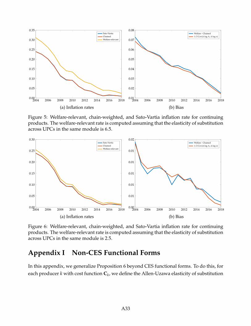
2004 2006 2008 2010 2012 2014 2016 20180.00

0.05

0.10

0.15

0.20

0.25

0.30

0.35Sato-VartiaChainedWelfare-relevant

(a) Inflation rates

2004 2006 2008 2010 2012 2014 2016 20180.01

0.02

0.03

0.04

0.05

0.06

0.07

0.08Welfare - Chained1/2 Cov(∆ log A, ∆ log x)

(b) Bias

Figure 5: Welfare-relevant, chain-weighted, and Sato-Vartia inflation rate for continuingproducts. The welfare-relevant rate is computed assuming that the elasticity of substitutionacross UPCs in the same module is 6.5.

2004 2006 2008 2010 2012 2014 2016 20180.00

0.05

0.10

0.15

0.20

0.25

0.30Sato-VartiaChainedWelfare-relevant

(a) Inflation rates

2004 2006 2008 2010 2012 2014 2016 20180.00

0.01

0.01

0.01

0.01

0.01

0.02Welfare - Chained1/2 Cov(∆ log A, ∆ log x)

(b) Bias

Figure 6: Welfare-relevant, chain-weighted, and Sato-Vartia inflation rate for continuingproducts. The welfare-relevant rate is computed assuming that the elasticity of substitutionacross UPCs in the same module is 2.5.

Appendix I Non-CES Functional Forms

In this appendix, we generalize Proposition 6 beyond CES functional forms. To do this, foreach producer k with cost function Ck, we define the Allen-Uzawa elasticity of substitution

A33

between inputs x and y as

θk(x, y) =Ckd2Ck/(dpxdpy)

(dCk/dpx)(dCk/dpy)=

εk(x, y)Ωky

,

where εk(x, y) is the elasticity of the demand by producer k for input x with respect to theprice py of input y, and Ωky is the expenditure share in cost of input y. For the householdk = 0, we use the household’s expenditure function in place of the cost function (wherethe Allen-Uzawa elasticities are disciplined by Hicksian cross-price elasticities and expen-diture shares).

Following Baqaee and Farhi (2019b), define the input-output substitution operator for pro-ducer k as

Φk(Ψ(i), Ψ(j)) = − ∑1≤x,y≤N+1+F

Ωkx[δxy + Ωky(θk(x, y)− 1)]ΨxiΨyj, (46)

(47)

where δxy is the Kronecker delta. Then, Proposition 6 generalizes as follows:

Proposition 14. At any point in time t, changes in the relevant variables are pinned down by thefollowing system of equations

d log pit = − ∑j∈N

Ψijtd log Ajt + ∑f∈F

ΨFi f td log λ f t. (48)

Changes in sales shares for goods and factors are

λitd log λit = ∑j∈0+N

λjtΦj

(−d log pt, Ψ(:,t),t

)(49)

+ CovΩ(0,:),t

(d log xt, Ψ(:,i),t

)+ CovΩ(0,:),t

(εt, Ψ(:,i),t)

(∑

k∈Nλktd log Akt

).

Changes in welfare-relevant variables are pinned down by the same set of differential equationsabove where the second line of (49) is set to zero and the boundary conditions are that Ω = Ωt1 andΨ = Ψt1 .

Since Φj shares many of the same properties as a covariance (it is bilinear and symmet-ric in its arguments, and is equal to zero whenever one of the arguments is a constant), theintuition for Proposition 14 is very similar to that of Proposition 6. Computing the equilib-rium response in Proposition 14 requires solving a linear system exactly as in Proposition6.

34