Welfare and Human Population in Austria

2013 | volume 1 issue 2 | 60–82

ISSN 2305-6991

BCSSS

systems. connecting matter, life, culture and technology

Welfare and Human Population in Austria

Maria T. Sanz Departamento de Ciencias Físicas, Matemáticas y de la Computación. Universidad CEU Cardenal Herrera. C/ San Bartolomé, 32. Al fara del Patr iarca (Valencia, Spain). [email protected]

Joan C. Micó Departament de Matemàtica Apl icada, Universi tat Pol i tècnica de València, Camí de Vera, s/n. Valencia (Spain), [email protected]

Antonio Caselles Departament de Matemàtica Apl icada, Universi tat de València. C/ Dr. Mol iner, 50, 46100 Burjassot (Valencia, Spain), antonio.casel [email protected]

David Soler Inst i tut Universi tar i de Matemàtica Pura i Apl icada. Universi tat Pol i tècnica de València, Camí de Vera, s/n, Valencia (Spain), [email protected]

Abstract: A model for a general human population dynamics is presented to approach the demographic stability problem. The main model variables are demographic variables per sexes (births, deaths, emigration, immigration and population) and the main well-being variables given by the UN: Human Development Index, Gender Development Index and Gender Empowerment Index. The model is presented in deterministic and stochastic formulations and it has been validated in the case of Austria in the 1999-2009 period.

Keywords: stochastic model; human population; well-being variables; Human Development Index; Gender Empowerment Index; Gender Development Index; demographically stable society.

This article is available from http://www.systems-journal.eu

© the author(s), publisher and licensee Bertalanffy Center for the Study of Systems Science http://www.bcsss.org

This is an open access article licensed under the Creative Commons Attribution 3.0 Austria License. Unrestricted use is permitted provided the original work is properly cited.

61

systems. connecting matter, life, culture and technology | 2013 | volume 1 | issue 2

1 Introduction

An abstract stochastic mathematical model to study the evolution of human population per sexes is presented in this paper. The model involves the three United Nations (UN) well-being variables used by Sanz et al. (2011): Human Development Index (HDI), Gender Development Index (GDI) and Gender Empowerment Index (GEM). The main advances of the model here presented with respect to the model by Sanz et al. (2011) are the stochastic formulation, the model validation for Austria and the application case to study the demographic stability.

The authors consider in this paper that the use of UN well-being variables in a mathematical model is essential to study the demographic stability. There are many problems corresponding to areas like environment, economy, health, education, labor force, culture, etc., which affect human well-being and demographic stability. Nevertheless, the literature review shows that there is little research about the dynamics of human population considering both sexes, covering demographic processes such as births, deaths, migration, and using well-being variables. The papers in which the authors found the use of well-being variables are:

- Mischler et al. (2002) consider the maturation variable to study the stability of solutions.

- Farkas (2004) focuses on the stability of McKendrick non-linear equations, which include fertility and mortality rates.

- Guo and Sun (2005) study how to optimize births with a McKendrick model through a dynamics programming-based method applied to the Chinese population.

- Alho and Spencer (2005) develop a steady population model, which considers marriages, divorces, as well as fertility rates. The model is based on the Leslie method of matrices, which is applied to different economic situations.

Other papers present models in which some kind of well-being variables related to economy, education, altruism or environmental pollution are considered:

- Hritonenko et al. (2008) present an age-structured demographic model considering variables like productivity, employment and income. They show that current technological trends in the United States are able to compensate negative demographic trends without increasing retirement age.

- Croix and Sommacal (2009) present an economic model where they show that increasing investment in the health field implies an increasing of the life expectancy at birth.

- Zajacova et al. (2009) study the effect of education on mortality. - Bréchet and Lambrecht (2009) develop an Overlapping Generations model where

the size of generations varies over time and converges towards a steady state. These authors introduce a new variable, altruism, which can also be considered a well-being variable. They use this model to study the influence of altruism, as well as renewable resources and economic movements on the population growth.

- Dubey (2010) proposes a nonlinear mathematical model to study the effect of environmental pollution on biomass resources and on human population dynamics. Finally, some other papers consider the UN well-being variables:

- Caselles et al. (2008) propose a deterministic human population dynamics model, where birth and death depend on HDI, although emigration and immigration rates depend on time.

62


- Sanz et al. (2011) present a deterministic model which is validated for Belgium in the 1997-2008 period.

- Sanz et al. (2014) present a stochastic human population-dynamics model per sexes, in which fertility and death rates depend on GDI. The model is validated for Spain in the 2000-2006 period. It is applied to test different strategies in different scenarios to select government inversions for the 2006-2015 period.

The benefit to use the UN well-being variables is their universality. In addition, they measure education, health, economy and female labor force. Thus, these variables can also help to solve problems involving the mentioned topics.

The definitions of the UN well-being variables are the following: HDI measures the average achievements of a given country with three variables:

A long and healthy life, measured by the life expectancy at birth. Education, given by the adult literacy rate and combined gross enrollment ratio of

primary, secondary and tertiary education. A worthy standard of life, given by the Gross Domestic Product (GDP) per capita in

Purchasing Power Parity (PPP) in U.S. dollars.

GDI is calculated from the same HDI variables, but they are differenced per sexes. In this case, GDP is replaced by male and female income.

GEM measures the role of women within society from:

Political participation and decision-making is calculated from the percentage of

female and male parliament members with seats. Economic participation and decision-making is measured by two variables:

percentage of men and women legislators, senior officials and managers, and percentage of female and male participation occupying professional and technical posts.

Power over economic resources which is provided by male and female incomes (PPP in US. dollars).

The objective of the presented model is to study the demographic stability related with a well-being improving. However, improving well-being implies creating a social environment, and the human capacities must be developed in the social environment (UNDP, 1990-2011). Education is the main human tool to create any social environment. Note that education helps to introduce new concepts and thoughts in society and to grow its potential. Delors (1996) considers education as one of the main engines of development and, as one of its functions, that humanity can achieve fully management of its own development. Some authors such as Zajacova et al. (2009) and Mukandavire et al. (2009) reinforce the idea of Delors (1996). They say that education is essential to meet the basic needs. In short, education represents a very important role for the development of a society. Education will lead to achieve a social environment with high well-being.

On the other hand, the demographically stable society concept is here defined as the tendency towards zero of the difference between births and deaths. The literature review agrees with this objective (Gil et al., 2006; World Commission on Environment and Development, 1988; Ehrlich and Ehrlich, 1994; Brown and Mitchell, 1998; Folch, 1998; Sartori, and Mazzoleni, 2003; Diamond, 2006).

63


Observe in addition, that the UN has created a Decade of Education for a Sustainable Future (2005-2014). Its aim is to give a solution to the population growth problem. They focus this problem from the field of education. UNESCO is the lead agency for promotion. The suggested goal is that educators must make a commitment to all types of education, both formal (from primary school to university) and informal (museums, media ...), pay systematic attention to the situation of the world in promoting attitudes and behavior favorable to the achievement of sustainable development (Gil et al., 2006).

Also, two very confusing concepts must be disambiguated: overpopulation and population growth. Ehrlich and Ehrlich (1994) note that "from the point of view of the habitability of the Earth, over-population of the rich countries is a more serious threat than the quick population growth in poor countries."

Following this idea, the overpopulation is defined as a condition in which the population density exceeds a threshold which causes a deterioration of the environment, a decrease in well-being or a decrease in population. On the other hand, population growth is set when the number of births contrasts against the number of deaths. Europe and Africa are two continents which help explaining these concepts. Population growth in Africa is much higher than in Europe, but Europe is much more populated than Africa. Overpopulated parts of the world have a higher consumption per capita than other and they contribute to the destruction of the environment. In this sense, the World Commission on Environment and Development (1988) discusses the implications of these two phenomena: "In many parts of the world, the population rates are growing but environmental resources cannot support them. Sometimes rates are surpassing all reasonable expectations of improvement in housing, health care, food security and energy supply."

Sachs (2008) notes that "the population growth world rate has declined but the world population increases quickly in regions with less capacity to ensure the health, stability and prosperity of the people (...). The world should adopt a set of measures to help stabilize world population through voluntary decisions, instead of maintaining the current path that probably will stand at nine billion or more in 2050."

Brown and Mitchell (1998) state that "population stabilization is an essential step to stop the destruction of natural resources and ensure the satisfaction of the basic needs of all people." That is, if we want a sustainable society, we will have to build a demographically stable society, and to do it, we should reduce current growth rates.

On the other hand, our model is abstract, i.e., it is transferable to any country. Moreover, it is a stochastic dynamic model in which the forecasts in each period are obtained by means of a confidence interval given by a minimum value and a maximum value with a specific probability. This way to present results provides a measure of its reliability, unlike deterministic models (Caselles, 1992). The methodology that has been used to construct our model is the General Modeling Methodology (GMM), proposed by A. Caselles, which is implemented by using SIGEM: the Complex-Systems based Programs’ Generator (Caselles, 1994, 2008). The GMM is a hypothetic-deductive methodology to construct complex models. This methodology has Data Mining Methods in some of its phases.

The rest of this paper is organized as follows. Section 2 presents and explains the model equations. Section 3 shows the model validation for the case of Austria in the 1999-2009 period. Section 4 suggests some strategies and scenarios to simulate the future and a way to determine the optimal strategy to achieve the proposed objective. Finally, Section 5 presents some conclusions and suggestions.

64


2 The model

First, all model variables are defined and listed by alphabetical order. We write the variables in this way:

XXXX Explanation variable [units of measure] (kind of variable)

Demographic variables: DEFE Female Deaths [population] (flow variable) DEMA Male Deaths [population] (flow variable) DETO Total Deaths [population] (auxiliary variable) EMIF Female Emigration [population] (flow variable) EMIG Total Emigration [population] (auxiliary variable) EMIM Male Emigration [population] (flow variable) POFI Female Population at the beginning of the year [population] (constant) POFL Female Population at the end of the year [population] (level variable) POMI Male Population at the beginning of the year [population] (constant) POML Male Population at the end of the year [population] (level variable) POPI Population at the beginning of the year [population] (auxiliary variable) POPL Population at the end of the year [population] (auxiliary variable) PRPF Female proportion [proportion] (auxiliary variable) PRPM Male proportion [proportion] (auxiliary variable) RDEF Female Death Rate [%] (auxiliary variable) RDEM Male Death Rate [%] (auxiliary variable) REMF Female emigration rate [%] (auxiliary variable) REMM Male emigration rate [%] (auxiliary variable) RFEF Female Fertility rate [births/female population] (auxiliary variable) RFEM Male Fertility rate [births/female population] (auxiliary variable) RINF Female immigration rate [%] (auxiliary variable) RINM Male immigration rate [%] (auxiliary variable) TEMI Initial year [time] (constant) TEMS Year [time] (level variable) XACF Female Births [population] (flow variable) XACI Total Births [population] (auxiliary variable) XACM Male Births [population] (flow variable) YNMF Female immigration [population] (flow variable) YNMI Total immigration [population] (auxiliary variable) YNMM Male immigration [population] (flow variable)

Human Development Index variables: GDPR Gross Domestic Product [PPP US$] (auxiliary variable) GRRR Gross Rate Registered to level primary secondary and tertiary [%] (auxiliary

variable) LAPO Literate Adult Population [%] (auxiliary variable) LEBI Life expectancy at birth [age] (auxiliary variable) XDII Human development Index initial value [%] (constant) XHDI Human development Index [%] (level variable) YEDU Educational Index [%] (auxiliary variable) YGDP Gross Domestic Product Index [%] (auxiliary variable)

65


YGRR Gross Rate Registered to level primary secondary and tertiary index [%] (auxiliary variable)

YLAP Literacy Rate Adults [%] (auxiliary variable)

Gender Development Index variables: GRFE Female Gross Registered to level primary, secondary and tertiary [%] (setting

variable) GRMA Male Gross Registered to level primary, secondary and tertiary [%] (setting

variable) LEBF Female life expectancy at birth [age] (setting variable) LEBM Male life expectancy at birth [age] (setting variable) RLAF Female literacy rate adults [%] (auxiliary variable) RLAM Male literacy rate adults [%] (auxiliary variable) RLIF Female literacy rate [%] (setting variable) RLIM Male literacy rate [%] (setting variable) YEID Equally Distributed Education Index [%] (auxiliary variable) YEFE Female Education Index [%] (auxiliary variable) YEMA Male Education Index [%] (auxiliary variable) YEVD Equally Distributed life expectancy at birth index [%] (auxiliary variable) YFEI Female income [PPP US$] (auxiliary variable) YFEM Female income [PPP US$] (auxiliary variable) YGRF Female Gross Rate Registered to level primary secondary and tertiary [%]

(auxiliary variable) YGRM Male Gross Rate Registered to level primary secondary and tertiary [%]

(auxiliary variable) YIIC Total income [PPP US$] (auxiliary variable) YIID Equally Distributed Income Index [%] (auxiliary variable) YIFE Female income index [%] (auxiliary variable) YIMA Male income index [%] (auxiliary variable) YLEB Life expectancy at birth index [%] (auxiliary variable) YLEF Female life expectancy at birth index [%] (auxiliary variable) YLEM Male life expectancy at birth index [%] (auxiliary variable) YMAI Male Income [PPP US$] (auxiliary variable) YMAL Male income [PPP US$] (setting variable) XGDI Gender Development Index [%] (level variable) XGII Gender Development Index initial value [%] (constant)

Gender Empowerment Index variables: EPID Percentage parliamentary representation [%] (auxiliary variable) EPIF Female Percentage parliamentary representation [%] (setting variable) EPIM Male Percentage parliamentary representation [%] (auxiliary variable) PAEF Female percentage shares of positions as legislators senior officials and

managers [%] (setting variable) PAEM Male percentage shares of positions as legislators senior officials and

managers [%] (auxiliary variable) PEID Average PEID [%] (auxiliary variable) PPPF Female percentage shares of professional and technical positions [%] (setting

variable)

66


PPPM Male percentage shares of professional and technical positions [%] (auxiliary variable)

PPTE PEID [%] (auxiliary variable) PPTI Professional index [%] (auxiliary variable) XAEE PEID within index [%] (auxiliary variable) XAEI PEID index senior [%] (auxiliary variable) XGEM Gender Empowerment Index [%] (level variable) XIPI Gender Empowerment Index initial value [%] (constant)

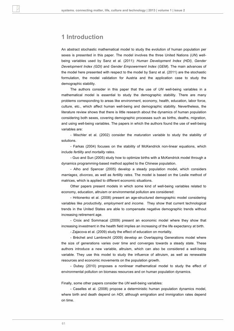
The relationships between these variables are displayed in the Forrester Diagram

(Forrester, 1961) in Figure 1. This is the characteristic diagram of System Dynamics and it is a translation of the Causal Diagram terminology that facilitates the writing of the equations when programming the model for a computer.

Figure 1: Forrester´s Diagram (1961)

In this diagram the variables are classified into different types:

Level variables: they require an initial value, which is an input variable, and the following values are updated. They are represented by a square or rectangle because they can be compared with tanks where a fluid is stored.

Flow variables: they can be compared with stopcocks that regulate the flow to or from a fluid tank. They are represented by a characteristic icon.

Auxiliary variables: intermediate variables that are used to calculate flows, or strict output variables (they aren’t used in other calculations and they are usually variables to optimize). They are represented by a circle or ellipse.

Setting variables: not controlled input variables. Control Variables: input variables whose value can be assigned by the decision

maker or the person that uses the model. Constants: system parameters with known and fixed value.

All input variables and constants are represented by a double line circle or ellipse. The Sources or Sinks are represented by a cloud (they are the source of the inflows or the end of the outflows of tanks).

67


The model reflects the influence of fertility, mortality, emigration, immigration on the male and female population, as well as the relation between fertility and mortality rates with well-being variables (HDI, GEM, GDI). These rates are calculated from input variables and the resulting population.

The model equations are the same than the presented ones in Sanz et al. (2011).

2.1 Fitting Rates

In order to validate the stochastic model, all fitted functions (fertility rates, mortality rates, emigration rates and immigration rates) must maintain the specific structure described by Caselles (1992, 2008). Now we show a short summary of this. Firstly, we calculate the mean value (represented by h in Sanz et al. (2014)) using the corresponding fitted function. Then we calculate the corresponding standard deviation (represented by s in Sanz et al. (2014)). All is made according to the method proposed by Caselles (1992, 2008). Thus, a generic variable such as Y would be obtained as: Y = h + s · ε(t). Being ε(t) a N(0,1), having h the following structure: h = a + b1T1 + b2T2 + … + bmTm ,

where a, b1, …, bm are parameters and T1, …, Tm are transformed functions of the independent variables, and being s calculated by using the following formula:

𝑠=𝑠𝑦𝑥1+1𝑛+𝜏′𝐶𝜏 (1)

Where syx is the standard deviation of regression, n is the number of data points, the

components of vector 𝜏 are the differences between the transformed functions Ti of the

independent variables and its respective average, and C is the inverse matrix of the variance-covariance matrix corresponding to the transformed functions. For instance, in Table 1 the following equation appears:

𝑅𝐹𝐸𝐹𝐻𝐷𝐼, 𝐺𝐷𝐼, 𝐺𝐸𝑀= 𝛼1+𝛽1·𝐻𝐷𝐼·𝐺𝐷𝐼·𝐺𝐸𝑀+𝛾1·𝐶𝑜𝑠𝜇1·𝐻𝐷𝐼·𝐺𝐷𝐼·𝐺𝐸𝑀 (2)

In this case, the transformed functions considered are: T1 = HDI·GDI·GEM and T2 = Cos(µ1 · HDI·GDI·GEM).

The historical data of demographic rates have been obtained from the database of the Austria Institute of Statistics for the 1998-2008 period. The information about the independent variables of such functions (HDI, GEM and GDI) are extracted from the Human Development Reports (UNDP) for the 1997-2007 period. In order to validate them, the analysis of the residuals and the calculation of the parameter R2 have been performed.

Next we present all the fitted functions for demographic rates: fertility, mortality, emigration and immigration rates. Tables 1 to 8 contain the needed data to write the stochastic formulation of the model and Figures 2 to 17 show the fitted functions (odd figures) and the residuals (even figures).

The mathematical structures shown in Tables 1 to 4 have been found by a trial and error process and the help of the functions finder and fitter tool Regint (Caselles, 1998, 2008). The work by Marchetti et al. (1996) demonstrates that fertility and death rates can be fitted by a logistic function or a sum of logistic functions. The data show a joint tendency to complete cycles (see Figures 2, 4, 6 and 8). A cycle can be formulated as an increasing logistics followed by a decreasing logistics. However, the available real data correspond to a short period, which prevents fitting the rates as a sum of logistics (too many parameters). The presented mathematical structures are the best option found to model the cycles for this

68


short period. Nevertheless, the fitted functions corresponding to the emigration rate and the immigration rate (Table 5 to 8) are single logistic functions. Finally the well-being indices, HDI, GDI or GEM are calculated with specific formulas detailed in UNDP (1990-2008).

𝑅𝐹𝐸𝐹𝐻𝐷𝐼, 𝐺𝐷𝐼, 𝐺𝐸𝑀= 𝛼1+𝛽1·𝐻𝐷𝐼·𝐺𝐷𝐼·𝐺𝐸𝑀+𝛾1·𝐶𝑜𝑠(𝜇1·𝐻𝐷𝐼·𝐺𝐷𝐼·𝐺𝐸𝑀)

RFEF αi βi µi γi

i=1 1.1348084388e2 -3.48271345e1 40.92001 -1.247076680

Matrix C Mean of transformed

function Estimation Error

30.79380.802930.802930.24080 T1=0.659464 T2=-0.303310

S=1.346669

Table 1: Parameters’ values for 𝑅𝐹𝐸𝐹𝐻𝐷𝐼, 𝐺𝐷𝐼, 𝐺𝐸𝑀

𝑅𝐹𝐸𝑀𝑡= 𝛼2+𝛽2·𝐻𝐷𝐼·𝐺𝐷𝐼·𝐺𝐸𝑀+𝛾2·𝐶𝑜𝑠(𝜇2·𝐻𝐷𝐼·𝐺𝐷𝐼·𝐺𝐸𝑀)

RFEM αi βi µi γi

i=2 1.235915776068e2 -4.3348629186382e1

36.054202 1.486311474769384

Matrix C Mean of transformed function Estimation Error

42.2975−2.1328−2.13280.32078 T1=0.659464 T2= 0.308286

S=1.598943

Table 2: Parameters’ values for 𝑅𝐹𝐸𝑀𝐻𝐷𝐼, 𝐺𝐷𝐼, 𝐺𝐸𝑀

Figure 3: Residuals (ordinate) of Female Birth Rate (abscise) in Austria, from the welfare variables in the 1998-2008 period.

Figure 2: Fitted function (solid line) and real data (dots) of Female Birth Rate in Austria, in the 1998-2008 period. R2=0.733401. For Kolmogorov-Smirnov's contrast, the theoretical deviation D(�,11)>0.13205, for any level of

significance �≥0.01. So, the normality hypothesis is accepted for the residuals of the model.

69


Table 3: Parameters’ values for 𝑅𝐷𝐸𝐹𝐻𝐷𝐼, 𝐺𝐷𝐼, 𝐺𝐸𝑀

𝑅𝐷𝐸𝑀𝑡=𝛼4+𝛽4·𝐻𝐷𝐼·𝐺𝐷𝐼·𝐺𝐸𝑀+𝛾4·𝐶𝑜𝑠(𝜇4·𝐻𝐷𝐼·𝐺𝐷𝐼·𝐺𝐸𝑀)

RDEM αi βi µi γi

i=4 1.339556717394 -1.8637323041928

2.340446 -7.84841086241e-1


1566260674227674227290239 T1=0.659464 T2=0.026886

S=0.001134

Table 4: Parameters’ values for𝑅𝐷𝐸𝑀𝐻𝐷𝐼, 𝐺𝐷𝐼, 𝐺𝐸𝑀

𝑅𝐷𝐸𝐹𝑡=𝛼3+𝛽3·𝐻𝐷𝐼·𝐺𝐷𝐼·𝐺𝐸𝑀+𝛾3·𝐶𝑜𝑠(𝜇3·𝐻𝐷𝐼·𝐺𝐷𝐼·𝐺𝐸𝑀)

RDEF αi βi µi γi

i=3 1.2976652477171e2 -4.900212547754e1

74.771696 9.367690707857e-1


28.35650.195380.195380.15909 T1=0.659464 T2=-0.108426

S=1.962267

Figure 4: Fitted function (solid line) and real data (dots) of Male Birth Rate in Austria, in the 1998-2008 period. R2 = 0.695521. For Kolmogorov-Smirnov's contrast, the theoretical deviation D(�,11)>0.160795, for any level of significance

�≥0.01. So, the normality hypothesis is accepted

for the residuals of the model.

Figure 5: Residuals (ordinate) of Male Birth Rate (abscise) in Austria, from the welfare variables in the 1998-2008 period.

Figure 7: Residuals (ordinate) of Female Death Rate (abscise) in Austria, from the welfare variables in the 1998-2008 period.

Figure 6: Fitted function (solid line) and real data (dots) of Female Death Rate in Austria, in the 1998-2008 period. R2 = 0.755094. For Kolmogorov-Smirnov's contrast, the

theoretical deviation D(�,11)>0.18025, for any level of

significance �≥0.01. So, the normality hypothesis is accepted for the residuals of the model.

70


Table 5: Parameters’ values for 𝑅𝐸𝑀𝐹𝑡

𝑅𝐸𝑀𝑀(𝑡)=𝜂6+𝛽61+𝛾6·𝑒𝑥𝑝𝛼6·𝑡−𝜇6

REMM ηi αi βi µi γi

i=6 1.19084177191e-1 -0.751511 -

1.6676285477e-2 2002 0.33799


C(0,0) = 26.705210812465 T1=0.275343 S=0.000037

Table 6: Parameters’ values for 𝑅𝐸𝑀𝑀𝑡

𝑅𝐸𝑀𝐹(𝑡)=𝜂5+𝛽51+𝛾5·𝑒𝑥𝑝𝛼5·𝑡−𝜇5

REMF ηi αi βi µi γi

i=5 7.43002178997e-3 1.25843 -

4.1734896411e-4 2000 58.1852


C(0,0) = 0.715271029174 T1=0.585007 S=0.000290

Figure 9: Residuals (ordinate) of Male Death Rate (abscise) in Austria, from the welfare variables in the 1998-2008 period.

Figure 8: Fitted function (solid line) and real data (dots) of Male Death Rate in Austria, in the 1998-2008 period. R2 = 0.854886. For Kolmogorov-Smirnov's contrast, the theoretical deviation D(�,11)>0.107544, for any level of

significance �≥0.01. So, the normality

hypothesis is accepted for the residuals of the model.

Figure 10: Fitted function (solid line) and real data (dots) of Female Emigration Rate in Austria, in the 2000-2008 period. R2=0.292092. For Kolmogorov-Smirnov's contrast, the theoretical deviation D(�,11)>0.154679,

for any level of significance �≥0.01. So, the normality


Figure 11: Residuals (ordinate) of Female Emigration Rate (abscise) in Austria, from the welfare variables in the 2000-2008 period.

71


Table 7: Parameters’ values for𝑅𝐼𝑁𝐹𝑡

𝑅𝐼𝑁𝑀(𝑡)=𝜂8+𝛽81+𝛾8·𝑒𝑥𝑝𝛼8·𝑡−𝜇8

RINM ηi αi βi µi γi

i=8

8.94551028026e-2 0.46795 1.19004999041e-1 2003 7.62838


C(0,0) = 3.321784726014 T1=0.551291 S=0.005436

Table 8: Parameters’ values for 𝑅𝐼𝑁𝑀𝑡

𝑅𝐼𝑁𝐹(𝑡)=𝜂7+𝛽71+𝛾7·𝑒𝑥𝑝𝛼7·𝑡−𝜇7

RINF ηi αi βi µi γi

i=7 7.71178515346e-1 0.405699 1.0507450342566 2003 10.2073


C(0,0) = 5.637004736678 T1=0.446858 S=0.045209

Figure 12: Fitted function (solid line) and real data (dots) of Male Emigration Rate in Austria, in the 2000-2008 period. R2=0.999447. For Kolmogorov-Smirnov's

contrast, the theoretical deviation D(�,11)>0.235617,

for any level of significance �≥0.01. So, the normality


Figure 13: Residuals (ordinate) of Male Emigration Rate (abscise) in Austria, from the welfare variables in the 2000-2008 period.

Figure 14: Fitted function (solid line) and real data (dots) of Female Immigration Rate in Austria, in the 1998-2008 period.. R2=0.926699. For Kolmogorov-Smirnov's contrast, the theoretical deviation D(�,11)>0.186044, for any level of significance

�≥0.01. So, the normality hypothesis is accepted for

the residuals of the model.

Figure 15: Residuals (ordinate) of Female Immigration Rate (abscise) in Austria, from the welfare variables in the 2000-2008 period.

72


3 Validation

The model validation in its two formulations, determinist and stochastic is presented in this section. The historical data used in this article to validate the model have been obtained from the Austria National Statistics Institute database in the 1999-2009 period. As mentioned in Section 1, the software tool used for model validation has been SIGEM.

3.1 Deterministic Validation

The model has been written as a set of finite difference equations and the solutions have been calculated with the Euler’s approximation, following Djidjeli et al. (1998), which explain that the Euler’s method is the more appropriate to solve this kind of equations. These equations have been programmed using SIGEM with the functions fitted in Section 2. Results have been obtained for the period 1999-2009.

Validation has been performed numerically, calculating the determination coefficients and testing the randomness of the residuals (Figures 18 and 19) and graphically, superposing the results obtained for each year and the historical data. The validation process has been considered successful due to three reasons:

The graphical superposition of historical and calculated data in the first years is very good.

The determination coefficients, R2, are very high. R2 is an index useful for global fitting between data sets:

𝑅2=𝑖𝑥𝑖−𝜇𝑥𝑦𝑖−𝜇𝑦2𝑖𝑥𝑖−𝜇𝑥2𝑖𝑦𝑖−𝜇𝑦2 (3)

where (xi ,yi) are the data to be compared, and µx and µy are the respective average values.

The maximum relative error does not exceed 5% (really it is lower enough).

Figure 16: Fitted function (solid line) and real data (dots) of Male Immigration Rate in Austria, in the 1998-2008 period. R2=0.94954. For Kolmogorov-Smirnov's contrast, the theoretical deviation D(�,11)>0.225751, for any level of significance �≥0.01. So, the normality hypothesis is accepted for the residuals of the model.

Figure 17: Residuals (ordinate) of Male Immigration Rate (abscise) in Austria, from the welfare variables in the 2000-2008 period.

73


Observe in Figures 18 and 19 that the model predictions show a one sided bias. This bias may be considered as negligible due to the scarce maximum relative error.

3.2 Stochastic Validation

The stochastic version of the model was the one used for simulation because it permits to determine the results’ reliability (each result is obtained with its respective confidence interval or with its respective average value and standard deviation).

The procedure to verify that the stochastic formulation of the model is validated is the following:

Observing that all the results have a normal distribution (for this purpose, SIGEM automatically programs a χ2 test).

Creating a (for instance) 95% confidence interval for each result and checking that all the historical data are within this interval.

The results corresponding to this validation type are presented in Figures 20 and 21. They confirm that the model is valid for Austria in the 1999-2009 period.

Figure 18: Forecast function (solid line) given by the model and real data (dots) for Austria’s Male Population, in the 1998-2009 period, R2= 0.935006, with 0.586985% of maximum relative error.

Figure 19: Forecast function (solid line) given by the model and real data (dots) for Austria’s Female Population, in the 1998-2009 period, R2=0.920724, with 0.836716% of maximum relative error.

Figure 20: Austrian Male Population 1999-2009. Minimum and Maximum values (solid lines) and real values (dots).

Figure 21: Austrian Female Population 1999-2009. Minimum and Maximum values (solid lines) and real values (dots).

74


4 Application: demographically stable society

Before making predictions with the model, we extrapolate all the input variables as a previous step to define relevant strategies and scenarios. To perform this extrapolation, firstly, the input variables are fitted with respect to time. All fitting functions are logistic sums. Logistic functions have the property that they can explain saturation of resources, and their use in demography has been proved to be very useful (Marchetti et al., 1996).

Next, these functions are extrapolated with confidence intervals using the Extrapol program (available in http://www.uv.es/caselles). The Extrapol program calculates the mean values (tendency values) and the limits of an interval at 95% confidence for each extrapolated year. Depending on each variable, an extrapolated value (maximum, minimum or mean) is assigned to each future scenario each year. Figures 22 to 24 show the extrapolation of the economic variables: Gross Domestic Product, Male Income and Female Income respectively.

Figure 22: GDPR, Gross Domestic Product Figure 23: YMAL, Male Income.

Figures 25 and 26 show the extrapolation of the health variables: Female Life Expectancy at Birth and Male Life Expectancy at Birth, respectively.

Figure 24: YFEM, Female Income.

75


Figure 25: LEBF, Female Life Expectancy at Birth. Figure 26: LEBM, Male Life Expectancy at Birth.

Figures 27 to 30 represent the extrapolation of the education variables: Male and Female Literacy Rate, Male and Female Gross Registered to level primary, secondary and tertiary, respectively.

Figure 27: RLIM, Male Literacy Rate. Figure 28: RLIF, Female Literacy Rate.

Finally, Figures 31 to 33 represent the extrapolation of the employment status for female’s variables: Female Percentage parliamentary representation, Female percentage shares of positions as legislator senior officials and managers and Female percentage shares of professional and technical positions, respectively.

Figure 29: GRMA, Male Gross Registered to level primary, secondary and tertiary.

Figure 30: GRFE, Female Gross Registered to level primary, secondary and tertiary.

76


Figure 33: PPPF, Female percentage shares of professional and technical positions.

Once everything is sketched and constructed, the model can be used to simulate the behavior of the system. The proposed objective is to determine how to reach a stable population.

Although the input variables are extrapolated up to the 2030 year, the concrete stated objective is to reach a stable population in 2025 due to the forecasts of this variable in the period 2025-2030 present a chaotic behavior that prevents any correct interpretation. The corresponding objective-variable is named as XSOSij where i=1, 2, 3 describe strategies and j= 1, 2, 3 describe scenarios. This variable computes the difference between births and deaths in each year of the 2010-2025 period.

In order to define some tentative strategies and scenarios, on the one hand, in the context of the model, the economic variables, GDPR, YMAL and YFEM, are assumed to be scenario variables due to the possible complexity of controlling them. On the other hand, the health and education variables: Life Expectancy per gender (LEBF, LEBM), Literate Rates per gender and Gross Enrolment ratio per gender (RLIM, RLIF, GRMA, GRFE) and employment status for females (EPIF, PAEF, PPPF) are assumed to be control variables, because relevant authorities may be able to carry out the mechanisms to assign a value to them over time.

Strategy 1: Empowering women within the labor scope. We increase investment in health and education over the detected trend and increase the participation rate of women in the labor scope over the detected trend. To do this, the average extrapolated values of education and the women position at the labor force variables are increased.

Figure 31: EPIF, Female Percentage parliamentary representation.

Figure 32: PAEF, Female percentage shares of positions as legislator senior officials and managers.

77


Strategy 2: Empowering women within the family. We increase investment in health and education over the detected trend and reduce the percentage of participation of women in the labor scope below the detected trend. To do this, the average extrapolated values of education variables are increased, and the values of the women position at the labor force are decreased.

Strategy 3: Maintaining the detected trend. In this case, the values of all control

variables keep the average extrapolated values.

GDPR YMAL YFEM

Scenario 1 ↑ ↑ ↑

Scenario 2 ↑ ↑ ↓

Scenario 3 ↑ ↑ ≈

Scenario 4 ↑ ↓ ↑

Scenario 5 ↑ ≈ ↑

Scenario 6 ↓ ↓ ↓

Scenario 7 ↓ ↓ ≈

Scenario 8 ≈ ↓ ↓

Scenario 9 ↓ ≈ ≈

Scenario 10 ≈ ↓ ≈

Scenario 11 ≈ ≈ ≈

Figure 34: Scenarios. Increasing the tendency of the economic variables: ↑.Decreasing the tendency of the economic variables: ↓. Keeping the tendency of the economic variables: ≈.

The variable to optimize is zopt1i

𝑧𝑜𝑝𝑡1𝑖=𝑗𝑋𝑆𝑂𝑆𝑖𝑗·𝑝𝑗 (4)

where the index i indicates the considered strategy and where pj are the probabilities that the experts assign to each one of the 11 considered scenarios (see Figure 34). The minimum value of this variable over time indicates which strategy is the best. In this paper we have chosen the value pj= 1/11 for all j, considering tentatively that all scenarios have the same probability to occur.

The optimal strategy for achieving the proposed goal is chosen by observing the evolution of zopt1i. The calculations are carried out with the simulator generated by SIGEM and Mathematica7.0. The results from the deterministic formulation are presented in Figure 35. The results from the stochastic formulation are presented in Figure 36. However, the conclusions can be better appreciated from the numerical results of the model stochastic formulation in Table 9.

78


Figure 35: Deterministic formulation. Forecasted average difference between births and deaths (zopt1). Strategy 1 (dots), Strategy 1: dots, Strategy 2: solid line, Strategy 3: dashed line, for period 2010-2025.

Figure 36: Stochastic formulation. Confidence intervals (95%) for the forecasted difference between births and deaths (zopt1). Strategy 1: dots, Strategy 2: solid line, Strategy 3: dashed line, for period 2010-2025.

Strategy 1 Strategy 2 Strategy 3 Year Minimum Maximum Minimum Maximum Minimum Maximum

2010 2618 3494 1513 2052 2163 2784

2011 2607 3459 1354 1864 1944 2639

2012 3061 3980 1365 1878 2358 3075

2013 2885 3925 1525 2086 2323 3112

2014 3092 4024 1637 2171 2325 3186

2015 3353 4156 1768 2284 2496 3273

2016 2690 3643 1692 2293 2412 3226

2017 2996 3854 1584 2114 2622 3461

2018 2485 3285 1697 2220 2280 3138

2019 2019 3704 1661 2248 2566 3334

2020 2041 2959 1944 2456 2542 3258

2021 1941 2859 1974 2486 2544 3260

2022 1341 2259 2144 2656 2538 3254

2023 741 1659 2314 2826 2640 3356

2024 441 1359 2344 2856 2627 3342

2025 441 1159 2454 2966 2629 3345

Table 9. Confidence intervals (95%) for the forecasted difference between births and deaths (zopt1).

79


Following the optimal strategy, i.e., Strategy 1, the conclusions are that, in Austria to achieve a stable society near 2025, Public Administrations would have to:

Invest over the observed trend in education (as needed to achieve the desired increase in gross enrollment rate and literacy);

Invest over the observed trend in health (as needed to achieve the desired increase in life expectancy at birth);

Increase the percentage of participation of women in the working life.

5 Conclusion

An abstract model has been presented to study the dynamics of a human population per genders. Three well-being variables have been included in the model. These variables are submitted by the United Nations: HDI, GDI and GEM. Through simulations, the model allows us to obtain the possible consequences of different strategies in different scenarios, giving the results along time either with their respective confidence intervals or with their respective mean and standard deviation.

The study has been performed with two model formulations: deterministic and stochastic. The deterministic one uses new generalized functions for emigration, immigration, birth and death rates, demonstrated being valid for Austria. On the other hand, the stochastic model seems the most appropriate for the problem posed in this paper, because it takes into account the “noise” or uncertainty, calculating the reliability of the results.

An application case referred to Austria is described. The main objective in this case is to obtain a stable population about 2025. Eleven scenarios and three strategies have been tentatively assumed as possible. Strategies are: investing in education, health and female labor force with priority (Strategy 1), investing in education and health with priority (Strategy 2) and, investing in the three fields with the same proportion (Strategy 3). Scenarios are the most interesting combination between three economic variables: gross domestic product, female income and male income. The obtained best strategy is Strategy 1 (for some tentative values given to the probabilities of the scenarios).

The current model could be expanded by using another UN well-being variable, the Human Poverty Index (HPI-2 for OECD countries and HPI-1 for countries outside the OECD). It would also be interesting to see if the HPI-1 is exchangeable with the HPI-2 in the corresponding formulas or not.

The resolution of the demographic sustainability problem can be tackled from other points of view, for example environmental or economic. This will involve designing a model with new variables related to fertility and mortality rates. For instance:

When tackling economic aspects, it is necessary to introduce in the model variables

related to migration, investments in other countries, human poverty, job security, etc.

When tackling environmental aspects, it is necessary to introduce variables related to energy, environmental management, demographic trends, etc.

Finally, an ambitious work would be to find a model considering several countries or regions, in order to set up the rates of migration in terms of the well-being variables of the involved countries.

80


References

Alho, J. M., Spencer, & B. D.(2005). Statistical Demography and Forecasting. Berlin: Springer.

Bréchet, T., & Lambrecht, S. (2009). Family Altruism with Renewable Resource and Population Growth. Mathematical Population Studies, 16 (1), 60-78.

Brown, L. R., Mitchell, J. (1998). Building a New Economy, in: L.R. Brown, C. Flavin, H. French (Eds.), The State of the World. New York: W.W. Norton.

Caselles, A. (1992). Simulation of Large Scale Stochastic Systems. In Cybernetics and Systems’92. R. Trappl (Eds.). Singapore: World Scientific. (pp. 221-228).

Caselles, A. (1994). Improvements in the Systems Based Program Generator SIGEM. Cybernetics and Systems: An International Journal, 25, 81-103.

Caselles, A. (1998). A tool for discovery by complex function fitting. In Cybernetics and Systems Research’98. R. Trappl (Eds.). Vienna: Austrian Society for Cybernetic Studies. (pp. 787-792).

Caselles, A. (Ed.). (2008) Modelización y simulación de sistemas complejos (Modeling and simulation of complex systems). Valencia (Spain): Universitat de València

Caselles, A., Micó, J.C., Soler, D., & Sanz, M.T. (2008). Population Growth and Social Well-being: A Dynamic Model Approach. Proceedings of the 7th Congress of the UES (Systems Science European Union). Lisbon (Portugal).

Croix, D., Sommacal, A. (2009). A Theory of Medical Effectiveness, Differential Mortality, Income Inequality and Growth for Pre-Industrial England. Mathematical Population Studies, 16(1), 2-3.

Delors, J. (Ed.). (1996). La educación encierra un tesoro. Unesco.

Diamond, J. (Ed.). (2006). Colapso. Debate.

Djidjeli A, W.G. Price A, P. Temarel A, & E.H. Twizell B. (1998). Partially implicit schemes for the numerical solutions of some non-linear differential equations. Applied Mathematics and Computation 96 (pp.177-207).

Dubey, B. (2010). A model for the effect of pollutant on human population dependent on a resource with environmental and health policy. Journal of Biological Systems, 18, 571-592.

Ehrlich, P.R. & Ehrlich, A.H. (Ed.). (1994). La explosión demográfica: El principal problema ecológico. Salvat.

Farkas, J. Z. (2004). Stability conditions for the non-linear McKendrick equations. Applied Mathematics and Computation, 156, 771-777.

Folch, R. (Ed.). (1998). Ambiente, emoción y ética. Ariel.

Forrester, J. W. (Ed.). (1961). Industrial dynamics. Cambridge: MIT Press.

Gil Pérez, D., Vilches, A., Toscano, J.C. & Macías, O. (2006). Década de la Educación para un futuro sostenible (2005-2014). Un necesario punto de inflexión en la atención a la situación del planeta. Revista Iberoamericana de Educación, 40, 125-178.

Guo, B.-Z. & Sun, B. (2005). Numerical solution to the optimal birth feedback control of a population dynamics: viscosity solution approach. Optimal Control Applications and Methods, 26, 229-254.

Hritonenko N. & Yatsenko Y. (2008). Can technological change sustain retirement in an aging population? Mathematical Population Studies, 15, 96-113.

Marchetti, C., Meyer, P. S., & Ausubel, J. H. (1996). Human Population Dynamics Revisited with the Logistic Model: How Much Can Be Modeled and Predicted? Technological Forecasting and Social Change, 52, 1-30.

Mischler, S., Perthame, B. & Ryzhik, L. (2002). Stability in a nonlinear population maturation model. Mathematical Models and Methods in Applied Sciences, 12, 1751-1772.

Mukandavire, Z., Garira, W. & Tchuenche, J.M. (2009). Modelling effects of public health educational campaigns on HIV/AIDS transmission dynamics. Applied Mathematical Modelling, 33, 2084-2095.

Sachs, J. (Ed.). (2008). Economía para un planeta abarrotado. Debate.

Sanz, M.T., Micó, J.C., Caselles, A. & Soler, D. (2011). Demography and Well-being. Proceedings of the 8th Congress of the UES (Systems Science European Union). Brussels (Belgium).

Sanz, M.T., Micó, J.C., Caselles, A. & Soler, D. (2014). A stochastic model for population and well-being dynamics. Journal of Mathematical Sociology. In press.

Sartori, G. & Mazzoleni, G. (2003). La Tierra explota. Superpoblación y Desarrollo. Taurus (ed).

UNDP (1990-2011). Human Development Report 1990. New York, Oxford: Oxford University Press, from http://hdr.undp.org/en

81


Zajacova, A., Goldman, N. & Rodriguez, G. (2009). Unobserved Heterogeneity Can Confound the Effect of Education on Mortality. Mathematical Population Studies, 16(2), 153-173.

World Commission on Environment and Development (Ed.). (1988). Nuestro Futuro Común. Madrid: Alianza.

About the Authors

Maria T. Sanz

Degree in Mathematics (2002-2007).

Doctor in Mathematics (2012).

Member of the Departamet de Didàctica de la MAtemàtica (Valencia, Spain). Lecturer at the University of Valencia since 2013, February. Member of SESGE (Sociedad Española de Sistemas Generales).

Her most important papers in this area are:

- Micó et al. (2008). A Side-by-Side Single Sex Age-Structured Human Population Dynamic Model: Exact Solution and Model Validation. Journal of Mathematical Sociology, ISSN: 0022-250X, Vol. 32, pp. 285-321.

- Sanz et al. (2014). A stochastic model for population and well-being dynamics. Journal of Mathematical Sociology. In press.

- Sanz et al. (2009). New trends in population dynamics. Revista Internacional De Sistemas, ISSN 0214-6533, Vol. 16, pp. 57-69.

- Micó et al. (2005). Un Modelo de von Foerster-Mckendrick para el Estudio de la Dinámica de Población Humana por Edades y Sexos. Revista Internacional de Sistemas, ISSN 0214-6533, Vol. 14, pp. 35-42.

Her most important meetings in this area are:

- Sanz et al. (2011). Demography and Well-being. Proceedings of the 8th Congress of the UES (Systems Science European Union). Brussels (Belgium).

- Caselles et al. (2008). Population Growth and Social Well-being: A Dynamic Model Approach. 7th Congress of the Systems Science European Union. Lisbon (Portugal).

Joan C. Micó Degree in Physics (1989). Doctor in Mathematics (2000). Member of the Departament de Matemàtica Aplicada (Valencia, Spain). Lecturer at the Polytechnic University of Valencia since 1997. His most important papers in this area are: - Micó JC et al. (2008). A side-by-side single sex age-structured human population dynamic model: exact solution and model validation. Journal of Mathematical Sociology (ISSN 0022-250X), vol. 32, pp. 285-321. - Micó JC, Soler D & Caselles C (2006). Age-structured human population dynamics. Journal of Mathematical Sociology (ISSN 0022-250X), vol. 30, pp. 1-31. - Micó JC el at. (2003). The multidimensional approach in systems dynamics. Modeling urban systems. Journal of Applied Systems Studies (ISSN 1466-7738), vol 3, pp. 644-655. His most important meetings in this area are: - Sanz et al. (2012). Well-being and Demographic Dynamics. International Conference on Complex Systems (ICCS'12). Agadir (Morocco). - Caselles et al. (2008). Population Growth and Social Well-being: A Dynamic Model Approach. 7th Congress of the Systems Science European Union. Lisbon (Portugal).

Antonio Caselles

Degree in Ingeniero Agrónomo (1970). Doctor in Ingeniero Agrónomo (1978).

82


Member of the Departament de Matemàtica Aplicada (Valencia, Spain). Lecturer at the University of Valencia since 1987. His most important papers in this area are: -Sanz, M.T., Micó, J.C., Caselles, A., Soler, D. (2011) Demography and Well-being. Proceedings of the 8th Congress of the UES (Systems Science European Union). Belgium. -Maria T. Sanz, Joan C. Micó, Antonio Caselles, David Soler, (2012). Welfare and Human Population in Austria. Proceedings of the 2012 European Meeting on Cybernetics and Systems Research. Vienna. Austria

- Micó, J.C., Caselles, A., Amigó, S., Cotolí, A., Sanz, M.T. (2012) The Body-Mind Problem from a Personality Relativity Theory Approach. Proceedings of the International Conference on Complex Systems (ICCS'12). Agadir, Morocco. 978-1-4673-4766-2/12/$31.00 c2012 IEEE. - María Sanz, Antonio Caselles, David Soler, Joan C. Micó. (2012) Well-being and Demographic Dynamics. Proceedings of the International Conference on Complex Systems (ICCS'12). Agadir, Morocco. 978-1-4673-4766-2/12/$31.00 c2012 IEEE. - Antonio Caselles (Keynote Speaker) (2012) Globalization and Sustainability. Can the present globalization process be reoriented? Proceedings of the International Conference on Complex Systems (ICCS'12). Agadir, Morocco. 978-1-4673-4766-2/12/$31.00 ©2012 IEEE

David Soler Degree in Mathematics (1986). Doctor in Mathematics (1995). Member of the institute of mathematics IUMPA (Valencia, Spain). Lecturer at the Polytechnic University of Valencia since 1986. His most important papers in this area are: - Micó JC et al. (2008). A side-by-side single sex age-structured human population dynamic model: exact solution and model validation. Journal of Mathematical Sociology (ISSN 0022-250X), vol. 32, pp. 285-321. - Micó JC, Soler D & Caselles C (2006). Age-structured human population dynamics. Journal of Mathematical Sociology (ISSN 0022-250X), vol. 30, pp. 1-31. - Micó JC el at. (2003). The multidimensional approach in systems dynamics. Modeling urban systems. Journal of Applied Systems Studies (ISSN 1466-7738), vol 3, pp. 644-655. His most important meetings in this area are: - Sanz et al. (2012). Well-being and Demographic Dynamics. International Conference on Complex Systems (ICCS'12). Agadir (Morocco). - Caselles et al. (2008). Population Growth and Social Well-being: A Dynamic Model Approach. 7th Congress of the Systems Science European Union. Lisbon (Portugal).

Welfare and Human Population in Austria

Documents

Transcript of Welfare and Human Population in Austria