CS361Week 6 - Wednesday

Last time

What did we talk about last time? Light Material Sensors

Questions?

Project 2

Back to Sensors

Real sensors

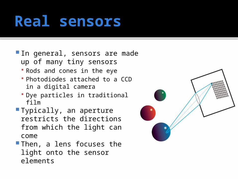
In general, sensors are made up of many tiny sensors Rods and cones in the eye Photodiodes attached to a CCD

in a digital camera Dye particles in traditional film

Typically, an aperture restricts the directions from which the light can come

Then, a lens focuses the light onto the sensor elements

Radiance

Irradiance sensors can't produce an image because they average over all directions

Lens + aperture = directionally specific

Consequently, the sensors measure radiance (L), the density of light per flow area AND incoming direction

Idealized sensors

In a rendering system, radiance is computed rather than measured

A radiance sample for each imaginary sensor element is made along a ray that goes through the point representing the sensor and point p, the center of projection for the perspective transform

The sample is computed by using a shading equation along the view ray v

Student Lecture: Lambertian, Gouraud, and Phong Shading

Shading

Shading equations

We need a mathematical equation to say what the color (radiance) at a particular pixel is

There are many equations to use and people still do research on how to make them better

Remember, these are all rule of thumb approximations and are only distantly related to physical law

Lambertian shading

Diffuse exitance Mdiff = cdiff EL cos θ Lambertian (diffuse) shading

assumes that outgoing radiance is (linearly) proportional to irradiance

Because diffuse radiance is assumed to be the same in all directions, we divide by π (explained later)

Final Lambertian radiance Ldiff = θcosdiffLEπ

c

Specular shading

Specular shading is dependent on the angles between the surface normal to the light vector and to the view vector

For the calculation, we compute h, the half vector half between v and l

vlvl

h

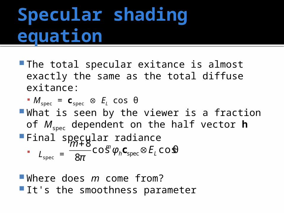
Specular shading equation The total specular exitance is almost exactly

the same as the total diffuse exitance: Mspec = cspec EL cos θ

What is seen by the viewer is a fraction of Mspec dependent on the half vector h

Final specular radiance Lspec =

Where does m come from? It's the smoothness parameter

θcoscos8

8spec Lh

m Eφπ

m

c

Implementing the shading equation

Final lighting is:

We want to implement this in shaders

The book goes into detail about how often it is computed Note that many terms can be

precomputed, only the ones with angles in them change

n

iLh

m Em

Li

1ispec

diff θcoscos8

8)( c

cv

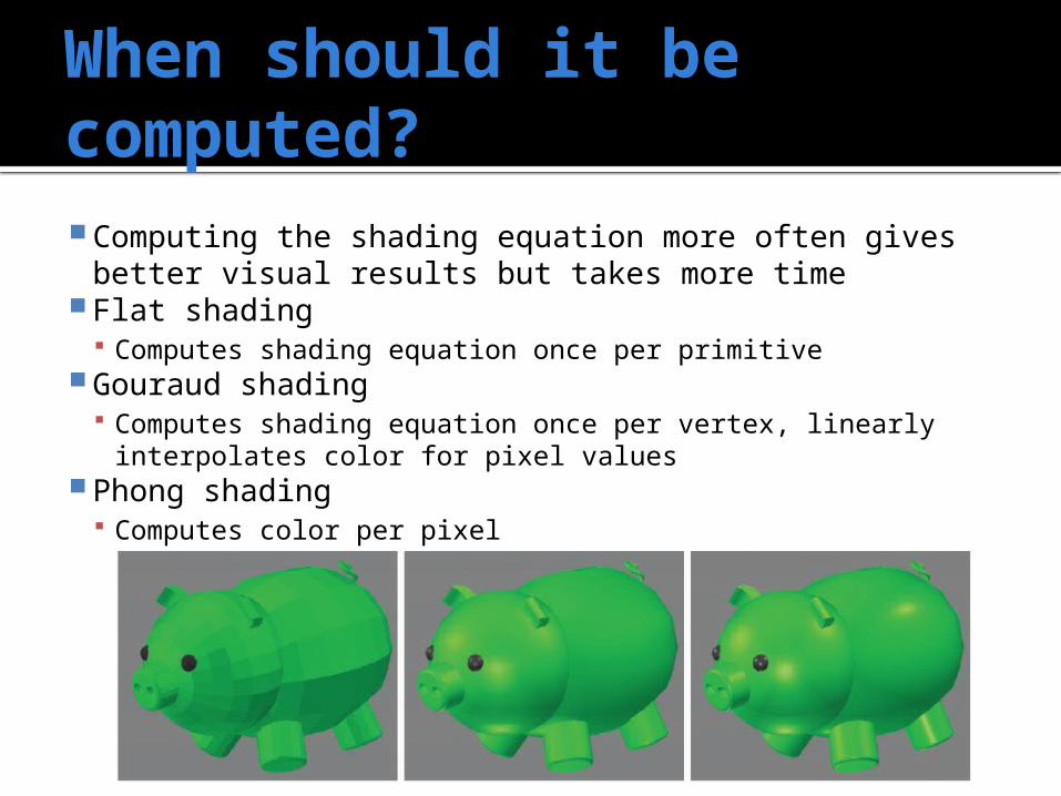
When should it be computed? Computing the shading equation more often gives

better visual results but takes more time Flat shading

Computes shading equation once per primitive Gouraud shading

Computes shading equation once per vertex, linearly interpolates color for pixel values

Phong shading Computes color per pixel

Aliasing

Aliasing

When sampling any continuous thing (image, sound, wave) into a discrete environment (like the computer), multiple samples can end up being indistinguishable from each other

This is called aliasing We can reduce aliasing by carefully

considering how sampling and reconstruction of the signal is done

Aliasing example

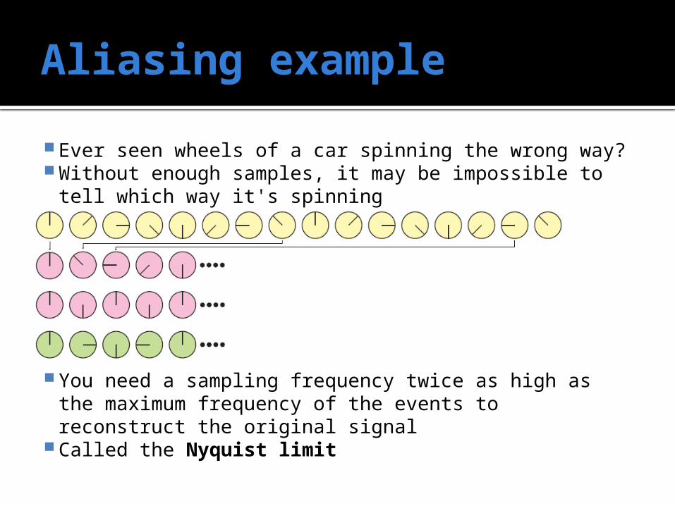
Ever seen wheels of a car spinning the wrong way? Without enough samples, it may be impossible to tell

which way it's spinning

You need a sampling frequency twice as high as the maximum frequency of the events to reconstruct the original signal

Called the Nyquist limit

Screen based antialiasing Jaggies are caused by insufficient sampling A simple method to increase sampling is full-

scene antialiasing, which essentially renders to a higher resolution and then averages neighboring pixels together

The accumulation buffer method is similar, except that the rendering is done with tiny offsets and the pixel values summed together

FSAA schemesA variety of FSAA schemes exist with different tradeoffs between quality and computational cost

A-buffer

For non-interactive render speeds, the A-buffer can be used

The A-buffer generates a coverage mask for each fragment for each pixel

Fragments are thrown away if they have z-buffer values that are higher than fragments with full coverage

Final pixel color is based on fragment merging

Multisample antialiasing

Supersampling techniques (like FSAA) are very expensive because the full shader has to run multiple times

Multisample antialiasing (MSAA) attempts to sample the same pixel multiple times but only run the shader once Expensive angle calculations can be done once

while different texture colors can be averaged Color samples are not averaged if they are off the

edge of a pixel

Performance, speed, the future Active research is still trying to find techniques with good

visual output and good computational performance Stochastic (random) sampling reduces the visual

repetition of some artifacts

Sharing samples between pixels can reduce overall cost

SharpDX Examples

Upcoming

Next time…

Review for Exam 1 Review all material covered so farExam 1 is Friday in class

Reminders

Keep working on Project 2, due Friday, March 1

Keep reading Chapter 5 Start reading Chapter 6