Week 2: Training Neural Networks - Hacettepeaykut/classes/... · BIL 722: Advanced Topics in...
211
BIL 722: Advanced Topics in Computer Vision (Deep Learning for Computer Vision) Erkut Erdem Spring 2016 Week 2: Training Neural Networks Visualization of the cat face neuron, from Le et al. Building high-level features using large-scale unsupervised learning, ICML 2012
Transcript of Week 2: Training Neural Networks - Hacettepeaykut/classes/... · BIL 722: Advanced Topics in...

BIL 722: Advanced Topics in Computer Vision (Deep Learning for Computer Vision)
Erkut Erdem
Spring 2016
Week 2: Training Neural Networks
Visualization of the cat face neuron, from Le et al. Building high-level features using large-scale unsupervised learning, ICML 2012

Today’s Lecture
• Part 1: Backpropagation and Neural Networks (Basics)
• Part 2: Training Neural Networks (Optimization, Learning tricks)
2

slide by Fei-FeiLi & Andrej Karpathy& Justin Johnson
Part 1
Backpropagationand
Neural Networks
3

slide by Fei-FeiLi & Andrej Karpathy& Justin Johnson
want
scores function
SVM loss
data loss + regularization
Where we are...
4

slide by Fei-FeiLi & Andrej Karpathy& Justin Johnson
(image credits to Alec Radford)
Optimization
5

slide by Fei-FeiLi & Andrej Karpathy& Justin Johnson
Gradient Descent
Numerical gradient: slow :(, approximate :(, easy to write :)Analytic gradient: fast :), exact :), error-prone :(
In practice: Derive analytic gradient, check your implementation with numerical gradient
6

slide by Fei-FeiLi & Andrej Karpathy& Justin Johnson
Computational Graph
x
W
* hingeloss
R
+ Ls (scores)
7

slide by Fei-FeiLi & Andrej Karpathy& Justin Johnson
Convolutional Network(AlexNet)
input imageweights
loss
8

slide by Fei-FeiLi & Andrej Karpathy& Justin Johnson
Neural Turing Machine
input tape
loss
9

slide by Fei-FeiLi & Andrej Karpathy& Justin Johnson
Neural Turing Machine
10
slide by Fei-FeiLi & Andrej Karpathy& Justin Johnson
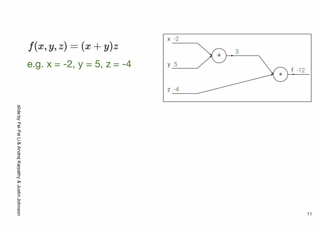
e.g. x = -2, y = 5, z = -4
11

slide by Fei-FeiLi & Andrej Karpathy& Justin Johnson
e.g. x = -2, y = 5, z = -4
Want:
12

slide by Fei-FeiLi & Andrej Karpathy& Justin Johnson
e.g. x = -2, y = 5, z = -4
Want:
13

slide by Fei-FeiLi & Andrej Karpathy& Justin Johnson
e.g. x = -2, y = 5, z = -4
Want:
14

slide by Fei-FeiLi & Andrej Karpathy& Justin Johnson
e.g. x = -2, y = 5, z = -4
Want:
15

slide by Fei-FeiLi & Andrej Karpathy& Justin Johnson
e.g. x = -2, y = 5, z = -4
Want:
16

slide by Fei-FeiLi & Andrej Karpathy& Justin Johnson
e.g. x = -2, y = 5, z = -4
Want:
17

slide by Fei-FeiLi & Andrej Karpathy& Justin Johnson
e.g. x = -2, y = 5, z = -4
Want:
18

slide by Fei-FeiLi & Andrej Karpathy& Justin Johnson
e.g. x = -2, y = 5, z = -4
Want:
19

slide by Fei-FeiLi & Andrej Karpathy& Justin Johnson
e.g. x = -2, y = 5, z = -4
Want:
Chain rule:
20

slide by Fei-FeiLi & Andrej Karpathy& Justin Johnson
e.g. x = -2, y = 5, z = -4
Want:
21

slide by Fei-FeiLi & Andrej Karpathy& Justin Johnson
e.g. x = -2, y = 5, z = -4
Want:
Chain rule:
22

slide by Fei-FeiLi & Andrej Karpathy& Justin Johnson
f
activations
23

slide by Fei-FeiLi & Andrej Karpathy& Justin Johnson
f
activations
“local gradient”
24

slide by Fei-FeiLi & Andrej Karpathy& Justin Johnson
f
activations
“local gradient”
gradients
25

slide by Fei-FeiLi & Andrej Karpathy& Justin Johnson
f
activations
gradients
“local gradient”
26

slide by Fei-FeiLi & Andrej Karpathy& Justin Johnson
f
activations
gradients
“local gradient”
27

slide by Fei-FeiLi & Andrej Karpathy& Justin Johnson
f
activations
gradients
“local gradient”
28

slide by Fei-FeiLi & Andrej Karpathy& Justin Johnson
Another example:
29

slide by Fei-FeiLi & Andrej Karpathy& Justin Johnson
Another example:
30

slide by Fei-FeiLi & Andrej Karpathy& Justin Johnson
Another example:
31

slide by Fei-FeiLi & Andrej Karpathy& Justin Johnson
Another example:
32

slide by Fei-FeiLi & Andrej Karpathy& Justin Johnson
Another example:
33

slide by Fei-FeiLi & Andrej Karpathy& Justin Johnson
Another example:
34

slide by Fei-FeiLi & Andrej Karpathy& Justin Johnson
Another example:
35

slide by Fei-FeiLi & Andrej Karpathy& Justin Johnson
Another example:
36

slide by Fei-FeiLi & Andrej Karpathy& Justin Johnson
Another example:
37

slide by Fei-FeiLi & Andrej Karpathy& Justin Johnson
Another example:
(-1)*(-0.20)=0.20
38

slide by Fei-FeiLi & Andrej Karpathy& Justin Johnson
Another example:
39

slide by Fei-FeiLi & Andrej Karpathy& Justin Johnson
Another example:
[local gradient] x [its gradient][1] x [0.2] = 0.2[1] x [0.2] = 0.2 (both inputs!)
40

slide by Fei-FeiLi & Andrej Karpathy& Justin Johnson
Another example:
41

slide by Fei-FeiLi & Andrej Karpathy& Justin Johnson
Another example:
[local gradient] x [its gradient]x0: [2] x [0.2] = 0.4w0: [-1] x [0.2] = -0.2
42

slide by Fei-FeiLi & Andrej Karpathy& Justin Johnson
sigmoid function
sigmoid gate
43
slide by Fei-FeiLi & Andrej Karpathy& Justin Johnson
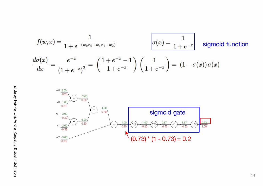
sigmoid function
sigmoid gate
(0.73) * (1 - 0.73) = 0.2
44

slide by Fei-FeiLi & Andrej Karpathy& Justin Johnson
Patterns in backward flow
add gate: gradient distributormax gate: gradient routermul gate: gradient… “switcher”?
45

slide by Fei-FeiLi & Andrej Karpathy& Justin Johnson
Gradients add at branches
+
46

slide by Fei-FeiLi & Andrej Karpathy& Justin Johnson
Implementation: forward/backward APIGraph (or Net) object. (Rough psuedo code)
47

slide by Fei-FeiLi & Andrej Karpathy& Justin Johnson
Implementation: forward/backward API
(x,y,z are scalars)
*
x
y
z
48

slide by Fei-FeiLi & Andrej Karpathy& Justin Johnson
Implementation: forward/backward API
(x,y,z are scalars)
*
x
y
z
49

slide by Fei-FeiLi & Andrej Karpathy& Justin Johnson
Example: Torch Layers
50

slide by Fei-FeiLi & Andrej Karpathy& Justin Johnson
Example: Torch Layers
=
51

slide by Fei-FeiLi & Andrej Karpathy& Justin Johnson
Example: Torch MulConstant
initialization
forward()
backward()
52

slide by Fei-FeiLi & Andrej Karpathy& Justin Johnson
Example: Caffe Layers
53

slide by Fei-FeiLi & Andrej Karpathy& Justin Johnson
Caffe Sigmoid Layer
*top_diff (chain rule)
54

slide by Fei-FeiLi & Andrej Karpathy& Justin Johnson
Gradients for vectorized code
f
“local gradient”
This is now the Jacobian matrix(derivative of each element of z w.r.t. each element of x)
(x,y,z are now vectors)
gradients
55

slide by Fei-FeiLi & Andrej Karpathy& Justin Johnson
Vectorized operations
f(x) = max(0,x)(elementwise)
4096-d input vector
4096-d output vector
56

slide by Fei-FeiLi & Andrej Karpathy& Justin Johnson
Vectorized operations
f(x) = max(0,x)(elementwise)
4096-d input vector
4096-d output vector
Q: what is the size of the Jacobian matrix?
Jacobian matrix
57

slide by Fei-FeiLi & Andrej Karpathy& Justin Johnson
max(0,x)(elementwise)
4096-d input vector
4096-d output vector
Q: what is the size of the Jacobian matrix?[4096 x 4096!]
Q2: what does it look like?
Vectorized operations
Jacobian matrix
f(x) = max(0,x)(elementwise)
58

slide by Fei-FeiLi & Andrej Karpathy& Justin Johnson
max(0,x)(elementwise)
100 4096-d input vectors
100 4096-d output vectors
Vectorized operations
in practice we process an entire minibatch (e.g. 100) of examples at one time:
i.e. Jacobian would technically be a[409,600 x 409,600] matrix :\
f(x) = max(0,x)(elementwise)
59

slide by Fei-FeiLi & Andrej Karpathy& Justin Johnson
Summary so far
- neural nets will be very large: no hope of writing down gradient formula by hand for all parameters
- backpropagation = recursive application of the chain rule along a computational graph to compute the gradients of all inputs/parameters/intermediates
- implementations maintain a graph structure, where the nodes implement the forward() / backward() API.
- forward: compute result of an operation and save any intermediates needed for gradient computation in memory
- backward: apply the chain rule to compute the gradient of the loss function with respect to the inputs.
60

slide by Fei-FeiLi & Andrej Karpathy& Justin Johnson
Neural Network: without the brain stuff
(Before) Linear score function:
61

slide by Fei-FeiLi & Andrej Karpathy& Justin Johnson
Neural Network: without the brain stuff
(Before) Linear score function:
(Now) 2-layer Neural Network
62

slide by Fei-FeiLi & Andrej Karpathy& Justin Johnson
Neural Network: without the brain stuff
(Before) Linear score function:
(Now) 2-layer Neural Network
x hW1 sW2
3072 100 10
63

slide by Fei-FeiLi & Andrej Karpathy& Justin Johnson
Neural Network: without the brain stuff
(Before) Linear score function:
(Now) 2-layer Neural Network
x hW1 sW2
3072 100 10
64

slide by Fei-FeiLi & Andrej Karpathy& Justin Johnson
Neural Network: without the brain stuff
(Before) Linear score function:
(Now) 2-layer Neural Networkor 3-layer Neural Network
65

slide by Fei-FeiLi & Andrej Karpathy& Justin Johnson
Full implementation of training a 2-layer Neural Network needs ~11 lines:
from @iamtrask, http://iamtrask.github.io/2015/07/12/basic-python-network/
66

slide by Fei-FeiLi & Andrej Karpathy& Justin Johnson
sigmoid activation function
67

slide by Fei-FeiLi & Andrej Karpathy& Justin Johnson 68

slide by Fei-FeiLi & Andrej Karpathy& Justin Johnson
Be very careful with your Brain analogies:
Biological Neurons:- Many different types- Dendrites can perform complex non-
linear computations- Synapses are not a single weight but
a complex non-linear dynamical system
- Rate code may not be adequate
[Dendritic Computation. London and Hausser]
69

slide by Fei-FeiLi & Andrej Karpathy& Justin Johnson 70
http://josephpcohen.com/w/visualizing-cnn-architectures-side-by-side-with-mxnet/
Felleman & van Essen, 1991
Human Visual System vs. ConvNets

slide by Fei-FeiLi & Andrej Karpathy& Justin Johnson
Activation Functions
Sigmoid
tanh tanh(x)
ReLU max(0,x)
Leaky ReLUmax(0.1x, x)
MaxoutELU
71

slide by Fei-FeiLi & Andrej Karpathy& Justin Johnson
Neural Networks: Architectures
“Fully-connected” layers“2-layer Neural Net”, or“1-hidden-layer Neural Net”
“3-layer Neural Net”, or“2-hidden-layer Neural Net”
72

slide by Fei-FeiLi & Andrej Karpathy& Justin Johnson
Example Feed-forward computation of a Neural Network
We can efficiently evaluate an entire layer of neurons.
73

slide by Fei-FeiLi & Andrej Karpathy& Justin Johnson
Example Feed-forward computation of a Neural Network
74

slide by Fei-FeiLi & Andrej Karpathy& Justin Johnson
Setting the number of layers and their sizes
more neurons = more capacity
75

slide by Fei-FeiLi & Andrej Karpathy& Justin Johnson
(you can play with this demo over at ConvNetJS: http://cs.stanford.edu/people/karpathy/convnetjs/demo/classify2d.html)
Do not use size of neural network as a regularizer. Use stronger regularization instead:
76
slide by Fei-FeiLi & Andrej Karpathy& Justin Johnson
Summary
- we arrange neurons into fully-connected layers- the abstraction of a layer has the nice property that it
allows us to use efficient vectorized code (e.g. matrix multiplies)
- neural networks are not really neural- neural networks: bigger = better (but might have to
regularize more strongly)
77

slide by Fei-FeiLi & Andrej Karpathy& Justin Johnson
reverse-mode differentiation (if you want effect of many things on one thing)
forward-mode differentiation (if you want effect of one thing on many things)
for many different x
for many different y
complex graph
inputs x outputs y
78

slide by Fei-FeiLi & Andrej Karpathy& Justin Johnson
Part 2
Training Neural Networks
79

slide by Fei-FeiLi & Andrej Karpathy& Justin Johnson
Mini-batch SGD
Loop:1. Sample a batch of data2. Forward prop it through the graph, get loss3. Backprop to calculate the gradients4. Update the parameters using the gradient
Where we are now...
80

slide by Fei-FeiLi & Andrej Karpathy& Justin Johnson
(image credits to Alec Radford)
Where we are now...
81

slide by Fei-FeiLi & Andrej Karpathy& Justin Johnson
Overview1.Onetimesetup
activationfunctions,preprocessing,weightinitialization,regularization,gradientchecking
2.Trainingdynamicsbabysittingthelearningprocess,parameterupdates,hyperparameter optimization
3.Evaluationmodelensembles
82

slide by Fei-FeiLi & Andrej Karpathy& Justin Johnson
Activation Functions
83

slide by Fei-FeiLi & Andrej Karpathy& Justin Johnson
Activation Functions
84

slide by Fei-FeiLi & Andrej Karpathy& Justin Johnson
Activation Functions
Sigmoid
tanh tanh(x)
ReLU max(0,x)
Leaky ReLUmax(0.1x, x)
Maxout
ELU
85

slide by Fei-FeiLi & Andrej Karpathy& Justin Johnson
Activation Functions
Sigmoid
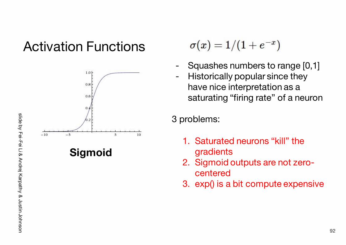
- Squashes numbers to range [0,1]- Historically popular since they
have nice interpretation as a saturating “firing rate” of a neuron
86

slide by Fei-FeiLi & Andrej Karpathy& Justin Johnson
Activation Functions
Sigmoid
- Squashes numbers to range [0,1]- Historically popular since they
have nice interpretation as a saturating “firing rate” of a neuron
3 problems:
1. Saturated neurons “kill” the gradients
87

slide by Fei-FeiLi & Andrej Karpathy& Justin Johnson
sigmoid gate
x
What happens when x = -10?What happens when x = 0?What happens when x = 10?
88

slide by Fei-FeiLi & Andrej Karpathy& Justin Johnson
Activation Functions
Sigmoid
- Squashes numbers to range [0,1]- Historically popular since they
have nice interpretation as a saturating “firing rate” of a neuron
3 problems:
1. Saturated neurons “kill” the gradients
2. Sigmoid outputs are not zero-centered
89

slide by Fei-FeiLi & Andrej Karpathy& Justin Johnson
Consider what happens when the input to a neuron (x) is always positive:
What can we say about the gradients on w?
90

slide by Fei-FeiLi & Andrej Karpathy& Justin Johnson
Consider what happens when the input to a neuron is always positive...
What can we say about the gradients on w?Always all positive or all negative :((this is also why you want zero-mean data!)
hypothetical optimal w vector
zig zag path
allowed gradient update directions
allowed gradient update directions
91
slide by Fei-FeiLi & Andrej Karpathy& Justin Johnson
Activation Functions
Sigmoid
- Squashes numbers to range [0,1]- Historically popular since they
have nice interpretation as a saturating “firing rate” of a neuron
3 problems:
1. Saturated neurons “kill” the gradients
2. Sigmoid outputs are not zero-centered
3. exp() is a bit compute expensive
92

slide by Fei-FeiLi & Andrej Karpathy& Justin Johnson
Activation Functions
tanh(x)
- Squashes numbers to range [-1,1]- zero centered (nice)- still kills gradients when saturated :(
[LeCun et al., 1991]
93

slide by Fei-FeiLi & Andrej Karpathy& Justin Johnson
Activation Functions - Computes f(x) = max(0,x)
- Does not saturate (in +region)- Very computationally efficient- Converges much faster than
sigmoid/tanh in practice (e.g. 6x)
ReLU(Rectified Linear Unit)
[Krizhevsky et al., 2012]
94

slide by Fei-FeiLi & Andrej Karpathy& Justin Johnson
Activation Functions
ReLU(Rectified Linear Unit)
- Computes f(x) = max(0,x)
- Does not saturate (in +region)- Very computationally efficient- Converges much faster than
sigmoid/tanh in practice (e.g. 6x)
- Not zero-centered output- An annoyance:
hint: what is the gradient when x < 0?
95

slide by Fei-FeiLi & Andrej Karpathy& Justin Johnson
ReLU gate
x
What happens when x = -10?What happens when x = 0?What happens when x = 10?
96

slide by Fei-FeiLi & Andrej Karpathy& Justin Johnson
DATA CLOUDactive ReLU
dead ReLUwill never activate => never update
97

slide by Fei-FeiLi & Andrej Karpathy& Justin Johnson
DATA CLOUDactive ReLU
dead ReLUwill never activate => never update
=> people like to initialize ReLU neurons with slightly positive biases (e.g. 0.01)
98

slide by Fei-FeiLi & Andrej Karpathy& Justin Johnson
Activation Functions
Leaky ReLU
- Does not saturate- Computationally efficient- Converges much faster than
sigmoid/tanh in practice! (e.g. 6x)- will not “die”.
[Mass et al., 2013][He et al., 2015]
99

slide by Fei-FeiLi & Andrej Karpathy& Justin Johnson
Activation Functions
Leaky ReLU
- Does not saturate- Computationally efficient- Converges much faster than
sigmoid/tanh in practice! (e.g. 6x)- will not “die”.
Parametric Rectifier (PReLU)
backprop into \alpha(parameter)
[Mass et al., 2013][He et al., 2015]
100

slide by Fei-FeiLi & Andrej Karpathy& Justin Johnson
Activation FunctionsExponential Linear Units (ELU)
- All benefits of ReLU- Does not die- Closer to zero mean outputs
- Computation requires exp()
[Clevert et al., 2015]
101

slide by Fei-FeiLi & Andrej Karpathy& Justin Johnson
Maxout “Neuron”- Does not have the basic form of dot product ->
nonlinearity- Generalizes ReLU and Leaky ReLU - Linear Regime! Does not saturate! Does not die!
Problem: doubles the number of parameters/neuron :(
[Goodfellow et al., 2013]
102

slide by Fei-FeiLi & Andrej Karpathy& Justin Johnson
Summary: In practice:
- Use ReLU. Be careful with your learning rates- Try out Leaky ReLU / Maxout / ELU- Try out tanh but don’t expect much- Don’t use sigmoid
103

slide by Fei-FeiLi & Andrej Karpathy& Justin Johnson
Data Preprocessing
104

slide by Fei-FeiLi & Andrej Karpathy& Justin Johnson
Step 1: Preprocess the data
(Assume X [NxD] is data matrix, each example in a row)
105
slide by Fei-FeiLi & Andrej Karpathy& Justin Johnson
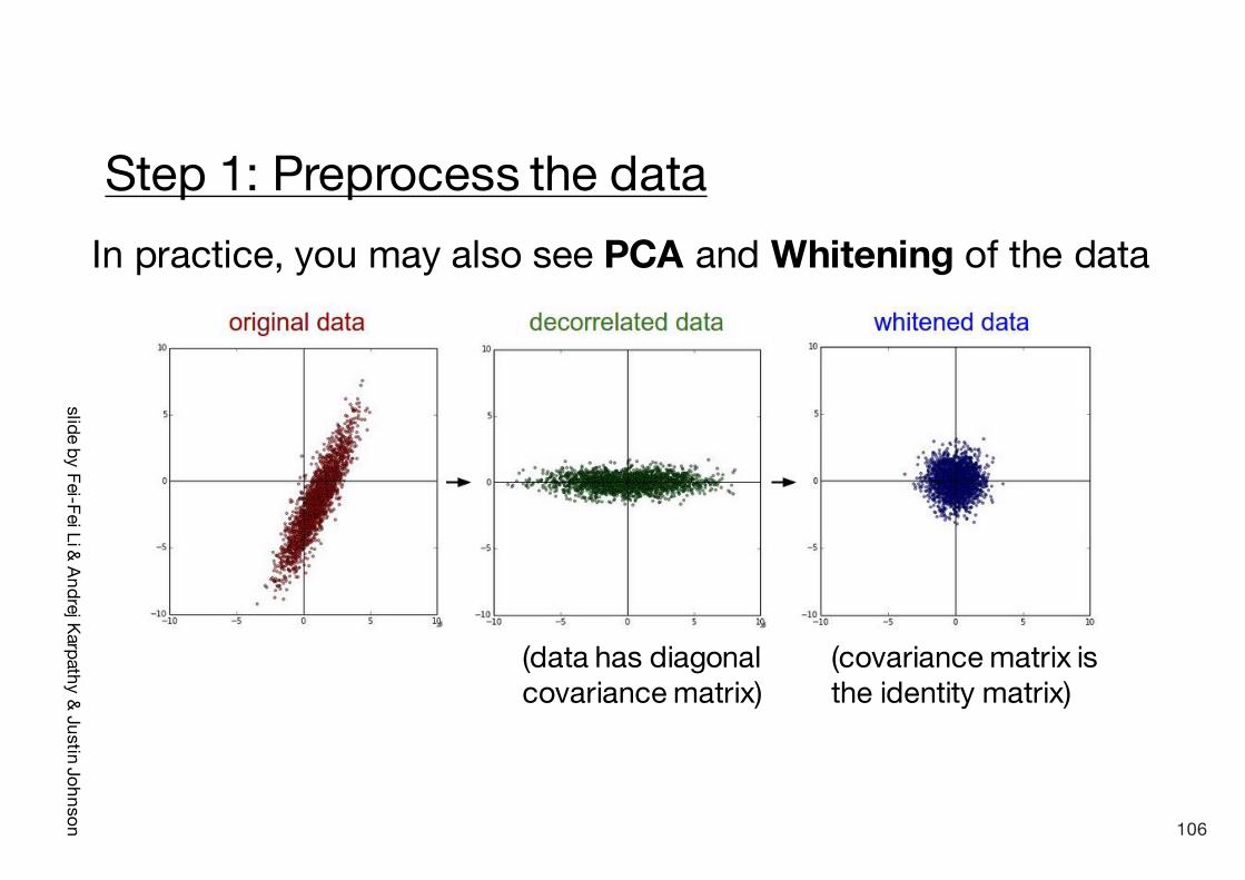
Step 1: Preprocess the dataIn practice, you may also see PCA and Whitening of the data
(data has diagonal covariance matrix)
(covariance matrix is the identity matrix)
106

slide by Fei-FeiLi & Andrej Karpathy& Justin Johnson
Summary: In practice for Images: center only
- Subtract the mean image (e.g. AlexNet)(mean image = [32,32,3] array)
- Subtract per-channel mean (e.g. VGGNet)(mean along each channel = 3 numbers)
e.g. consider CIFAR-10 example with [32,32,3] images
Not common to normalize variance, to do PCA or whitening
107

slide by Fei-FeiLi & Andrej Karpathy& Justin Johnson
Weight Initialization
108

slide by Fei-FeiLi & Andrej Karpathy& Justin Johnson
- Q: what happens when W=0 init is used?
109

slide by Fei-FeiLi & Andrej Karpathy& Justin Johnson
- First idea: Small random numbers (gaussian with zero mean and 1e-2 standard deviation)
110

slide by Fei-FeiLi & Andrej Karpathy& Justin Johnson
- First idea: Small random numbers (gaussian with zero mean and 1e-2 standard deviation)
Works ~okay for small networks, but can lead to non-homogeneous distributions of activations across the layers of a network.
111

slide by Fei-FeiLi & Andrej Karpathy& Justin Johnson
Lets look at some activation statistics
E.g. 10-layer net with 500 neurons on each layer, using tanhnon-linearities, and initializing as described in last slide.
112

slide by Fei-FeiLi & Andrej Karpathy& Justin Johnson 113

slide by Fei-FeiLi & Andrej Karpathy& Justin Johnson
All activations become zero!
Q: think about the backward pass. What do the gradients look like?
Hint: think about backward pass for a W*X gate.
114

slide by Fei-FeiLi & Andrej Karpathy& Justin Johnson
Almost all neurons completely saturated, either -1 and 1. Gradients will be all zero.
*1.0 instead of *0.01
115

slide by Fei-FeiLi & Andrej Karpathy& Justin Johnson
“Xavier initialization”[Glorot et al., 2010]
Reasonable initialization.(Mathematical derivation assumes linear activations)
116

slide by Fei-FeiLi & Andrej Karpathy& Justin Johnson
but when using the ReLU nonlinearity it breaks.
117

slide by Fei-FeiLi & Andrej Karpathy& Justin Johnson
He et al., 2015(note additional /2)
118

slide by Fei-FeiLi & Andrej Karpathy& Justin Johnson
He et al., 2015(note additional /2)
119

slide by Fei-FeiLi & Andrej Karpathy& Justin Johnson
Proper initialization is an active area of research…Understanding the difficulty of training deep feedforward neural networksby Glorot and Bengio, 2010
Exact solutions to the nonlinear dynamics of learning in deep linear neural networks by Saxe et al, 2013
Random walk initialization for training very deep feedforward networks by Sussillo and Abbott, 2014
Delving deep into rectifiers: Surpassing human-level performance on ImageNetclassification by He et al., 2015
Data-dependent Initializations of Convolutional Neural Networks by Krähenbühl et al., 2015
All you need is a good init, Mishkin and Matas, 2015…
120

slide by Fei-FeiLi & Andrej Karpathy& Justin Johnson
Batch Normalization“you want unit gaussian activations? just make them so.”
[Ioffe and Szegedy, 2015]
consider a batch of activations at some layer. To make each dimension unit gaussian, apply:
this is a vanilla differentiable function...
121

slide by Fei-FeiLi & Andrej Karpathy& Justin Johnson
Batch Normalization“you want unit gaussian activations? just make them so.”
[Ioffe and Szegedy, 2015]
XN
D
1. compute the empirical mean and variance independently for each dimension.
2. Normalize
122

slide by Fei-FeiLi & Andrej Karpathy& Justin Johnson
Batch Normalization [Ioffe and Szegedy, 2015]
FC
BN
tanh
FC
BN
tanh
...
Usually inserted after Fully Connected / (or Convolutional, as we’ll see soon) layers, and before nonlinearity.
Problem: do we necessarily want a unit gaussian input to a tanh layer?
123

slide by Fei-FeiLi & Andrej Karpathy& Justin Johnson
Batch Normalization [Ioffe and Szegedy, 2015]
And then allow the network to squash the range if it wants to:
Note, the network can learn:
to recover the identity mapping.
Normalize:
124

slide by Fei-FeiLi & Andrej Karpathy& Justin Johnson
Batch Normalization [Ioffe and Szegedy, 2015]
- Improves gradient flow through the network
- Allows higher learning rates- Reduces the strong
dependence on initialization- Acts as a form of regularization
in a funny way, and slightly reduces the need for dropout, maybe
125

slide by Fei-FeiLi & Andrej Karpathy& Justin Johnson
Batch Normalization [Ioffe and Szegedy, 2015]
Note: at test time BatchNorm layer functions differently:
The mean/std are not computed based on the batch. Instead, a single fixed empirical mean of activations during training is used.
(e.g. can be estimated during training with running averages)
126

slide by Fei-FeiLi & Andrej Karpathy& Justin Johnson
Babysitting the Learning Process
127

slide by Fei-FeiLi & Andrej Karpathy& Justin Johnson
Step 1: Preprocess the data
(Assume X [NxD] is data matrix, each example in a row)
128

slide by Fei-FeiLi & Andrej Karpathy& Justin Johnson
Step 2: Choose the architecture:say we start with one hidden layer of 50 neurons:
input layer hidden layer
output layerCIFAR-10 images, 3072 numbers
10 output neurons, one per class
50 hidden neurons
129

slide by Fei-FeiLi & Andrej Karpathy& Justin Johnson
Double check that the loss is reasonable:
returns the loss and the gradient for all parameters
disable regularizationloss ~2.3.“correct “ for 10 classes
130

slide by Fei-FeiLi & Andrej Karpathy& Justin Johnson
Double check that the loss is reasonable:
crank up regularization
loss went up, good. (sanity check)
131

slide by Fei-FeiLi & Andrej Karpathy& Justin Johnson
Lets try to train now…
Tip: Make sure that you can overfit very small portion of the training data The above code:
- take the first 20 examples from CIFAR-10
- turn off regularization (reg = 0.0)- use simple vanilla ‘sgd’
132
slide by Fei-FeiLi & Andrej Karpathy& Justin Johnson
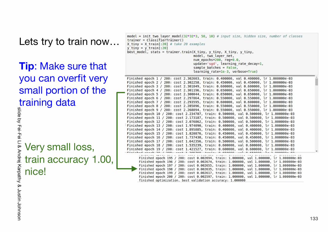
Lets try to train now…
Tip: Make sure that you can overfit very small portion of the training data
Very small loss, train accuracy 1.00, nice!
133

slide by Fei-FeiLi & Andrej Karpathy& Justin Johnson
Lets try to train now…
I like to start with small regularization and find learning rate that makes the loss go down.
134
slide by Fei-FeiLi & Andrej Karpathy& Justin Johnson
Lets try to train now…
I like to start with small regularization and find learning rate that makes the loss go down. Loss barely changing
135

slide by Fei-FeiLi & Andrej Karpathy& Justin Johnson
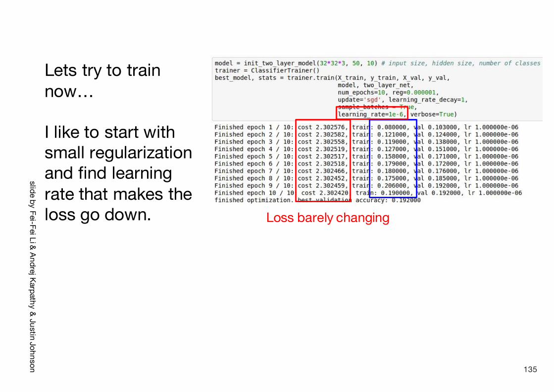
Lets try to train now…
I like to start with small regularization and find learning rate that makes the loss go down.
loss not going down:learning rate too low
Loss barely changing: Learning rate is probably too low
136

slide by Fei-FeiLi & Andrej Karpathy& Justin Johnson
Lets try to train now…
I like to start with small regularization and find learning rate that makes the loss go down.
loss not going down:learning rate too low
Loss barely changing: Learning rate is probably too low
Notice train/val accuracy goes to 20% though, what’s up with that? (remember this is softmax)
137

slide by Fei-FeiLi & Andrej Karpathy& Justin Johnson
Lets try to train now…
I like to start with small regularization and find learning rate that makes the loss go down.
loss not going down:learning rate too low
Okay now lets try learning rate 1e6. What could possibly go wrong?
138

slide by Fei-FeiLi & Andrej Karpathy& Justin Johnson
cost: NaN almost always means high learning rate...
Lets try to train now…
I like to start with small regularization and find learning rate that makes the loss go down.
loss not going down:learning rate too lowloss exploding:learning rate too high
139

slide by Fei-FeiLi & Andrej Karpathy& Justin Johnson
Lets try to train now…
I like to start with small regularization and find learning rate that makes the loss go down.
loss not going down:learning rate too lowloss exploding:learning rate too high
3e-3 is still too high. Cost explodes….
=> Rough range for learning rate we should be cross-validating is somewhere [1e-3 … 1e-5]
140

slide by Fei-FeiLi & Andrej Karpathy& Justin Johnson
Hyperparameter Optimization
141

slide by Fei-FeiLi & Andrej Karpathy& Justin Johnson
Cross-validation strategyI like to do coarse -> fine cross-validation in stages
First stage: only a few epochs to get rough idea of what params workSecond stage: longer running time, finer search… (repeat as necessary)
Tip for detecting explosions in the solver: If the cost is ever > 3 * original cost, break out early
142

slide by Fei-FeiLi & Andrej Karpathy& Justin Johnson
For example: run coarse search for 5 epochs
nice
note it’s best to optimize in log space!
143

slide by Fei-FeiLi & Andrej Karpathy& Justin Johnson
Now run finer search...adjust range
53% - relatively good for a 2-layer neural net with 50 hidden neurons.
144

slide by Fei-FeiLi & Andrej Karpathy& Justin Johnson
Now run finer search...adjust range
53% - relatively good for a 2-layer neural net with 50 hidden neurons.
But this best cross-validation result is worrying. Why?
145

slide by Fei-FeiLi & Andrej Karpathy& Justin Johnson
Random Search vs. Grid Search
Random Search for Hyper-Parameter OptimizationBergstra and Bengio, 2012
146
slide by Fei-FeiLi & Andrej Karpathy& Justin Johnson
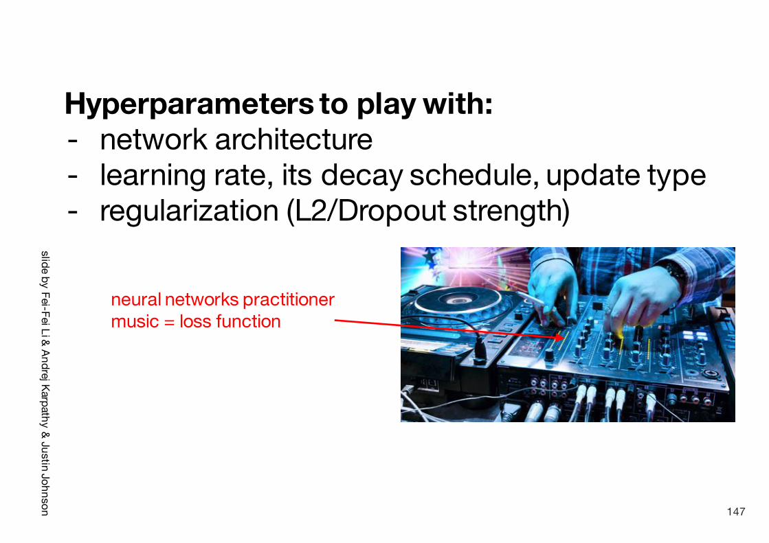
Hyperparameters to play with:- network architecture- learning rate, its decay schedule, update type- regularization (L2/Dropout strength)
neural networks practitionermusic = loss function
147

slide by Fei-FeiLi & Andrej Karpathy& Justin Johnson
Monitor and visualize the loss curve
148

slide by Fei-FeiLi & Andrej Karpathy& Justin Johnson
Loss
time
149

slide by Fei-FeiLi & Andrej Karpathy& Justin Johnson
Loss
time
Bad initializationa prime suspect
150

slide by Fei-FeiLi & Andrej Karpathy& Justin Johnson
Monitor and visualize the accuracy:
big gap = overfitting=> increase regularization strength?
no gap=> increase model capacity?
151

slide by Fei-FeiLi & Andrej Karpathy& Justin Johnson
Track the ratio of weight updates / weight magnitudes:
ratio between the values and updates: ~ 0.0002 / 0.02 = 0.01 (about okay)want this to be somewhere around 0.001 or so
152

slide by Fei-FeiLi & Andrej Karpathy& Justin Johnson
So far..We looked in detail at:
- Activation Functions (use ReLU)- Data Preprocessing (images: subtract mean)- Weight Initialization (use Xavier init)- Batch Normalization (use)- Babysitting the Learning process- Hyperparameter Optimization
(random sample hyperparams, in log space when appropriate)
153

slide by Fei-FeiLi & Andrej Karpathy& Justin Johnson
NOW
- Parameter update schemes- Learning rate schedules- Model ensembles- More on regularization: Dropout
154

slide by Fei-FeiLi & Andrej Karpathy& Justin Johnson
Parameter Updates
155

slide by Fei-FeiLi & Andrej Karpathy& Justin Johnson
Training a neural network, main loop:
156

slide by Fei-FeiLi & Andrej Karpathy& Justin Johnson
simple gradient descent updatenow: complicate.
Training a neural network, main loop:
157

slide by Fei-FeiLi & Andrej Karpathy& Justin Johnson
Image credits: Alec Radford
158

slide by Fei-FeiLi & Andrej Karpathy& Justin Johnson
Suppose loss function is steep vertically but shallow horizontally:
Q: What is the trajectory along which we converge towards the minimum with SGD?
159

slide by Fei-FeiLi & Andrej Karpathy& Justin Johnson
Suppose loss function is steep vertically but shallow horizontally:
Q: What is the trajectory along which we converge towards the minimum with SGD?
160

slide by Fei-FeiLi & Andrej Karpathy& Justin Johnson
Suppose loss function is steep vertically but shallow horizontally:
Q: What is the trajectory along which we converge towards the minimum with SGD? very slow progress along flat direction, jitter along steep one
161

slide by Fei-FeiLi & Andrej Karpathy& Justin Johnson
Momentum update
- Physical interpretation as ball rolling down the loss function + friction (mu coefficient).- mu = usually ~0.5, 0.9, or 0.99 (Sometimes annealed over time, e.g. from 0.5 -> 0.99)
162

slide by Fei-FeiLi & Andrej Karpathy& Justin Johnson
Momentum update
- Allows a velocity to “build up” along shallow directions- Velocity becomes damped in steep direction due to quickly changing
sign
163

slide by Fei-FeiLi & Andrej Karpathy& Justin Johnson
SGD vsMomentum notice momentum
overshooting the target, but overall getting to the minimum much faster.
164

slide by Fei-FeiLi & Andrej Karpathy& Justin Johnson
Nesterov Momentum update
gradientstep
momentumstep actual step
Ordinary momentum update:
165

slide by Fei-FeiLi & Andrej Karpathy& Justin Johnson
Nesterov Momentum update
gradientstep
momentumstep actual step
momentumstep
“lookahead” gradient step (bit different than original)
actual step
Momentum update Nesterov momentum update
166

slide by Fei-FeiLi & Andrej Karpathy& Justin Johnson
Nesterov Momentum update
gradientstep
momentumstep actual step
momentumstep
“lookahead” gradient step (bit different than original)
actual step
Momentum update Nesterov momentum update
Nesterov: the only difference...
167

slide by Fei-FeiLi & Andrej Karpathy& Justin Johnson
Nesterov Momentum updateSlightly inconvenient… usually we have :
Variable transform and rearranging saves the day:Replace all thetas with phis, rearrange and obtain:
168

slide by Fei-FeiLi & Andrej Karpathy& Justin Johnson
nag = NesterovAccelerated Gradient
169

slide by Fei-FeiLi & Andrej Karpathy& Justin Johnson
AdaGrad update
Added element-wise scaling of the gradient based on the historical sum of squares in each dimension
[Duchi et al., 2011]
170

slide by Fei-FeiLi & Andrej Karpathy& Justin Johnson
Q: What happens with AdaGrad?
AdaGrad update
171

slide by Fei-FeiLi & Andrej Karpathy& Justin Johnson
Q2: What happens to the step size over long time?
AdaGrad update
172

slide by Fei-FeiLi & Andrej Karpathy& Justin Johnson
RMSProp update [Tieleman and Hinton, 2012]
173

slide by Fei-FeiLi & Andrej Karpathy& Justin Johnson
Introduced in a slide in Geoff Hinton’s Coursera class, lecture 6
Cited by several papers as:
174

slide by Fei-FeiLi & Andrej Karpathy& Justin Johnson
adagradrmsprop
175

slide by Fei-FeiLi & Andrej Karpathy& Justin Johnson
Adam update [Kingma and Ba, 2014]
(incomplete, but close)
176

slide by Fei-FeiLi & Andrej Karpathy& Justin Johnson
Adam update [Kingma and Ba, 2014]
(incomplete, but close)
momentum
RMSProp-like
Looks a bit like RMSProp with momentum
177

slide by Fei-FeiLi & Andrej Karpathy& Justin Johnson
Adam update [Kingma and Ba, 2014]
(incomplete, but close)
momentum
RMSProp-like
Looks a bit like RMSProp with momentum
178

slide by Fei-FeiLi & Andrej Karpathy& Justin Johnson
Adam update [Kingma and Ba, 2014]
RMSProp-like
bias correction(only relevant in first few iterations when t is small)
momentum
The bias correction compensates for the fact that m,v are initialized at zero and need some time to “warm up”.
179

slide by Fei-FeiLi & Andrej Karpathy& Justin Johnson
SGD, SGD+Momentum, Adagrad, RMSProp, Adam all have learning rate as a hyperparameter.
Q: Which one of these learning rates is best to use?
180

slide by Fei-FeiLi & Andrej Karpathy& Justin Johnson
SGD, SGD+Momentum, Adagrad, RMSProp, Adam all have learning rate as a hyperparameter.
=> Learning rate decay over time!
step decay: e.g. decay learning rate by half every few epochs.
exponential decay:
1/t decay:
181

slide by Fei-FeiLi & Andrej Karpathy& Justin Johnson
Second order optimization methodssecond-order Taylor expansion:
Solving for the critical point we obtain the Newton parameter update:
Q: what is nice about this update?
182

slide by Fei-FeiLi & Andrej Karpathy& Justin Johnson
Second order optimization methodssecond-order Taylor expansion:
Solving for the critical point we obtain the Newton parameter update:
Q2: why is this impractical for training Deep Neural Nets?
notice: no hyperparameters! (e.g. learning rate)
183

slide by Fei-FeiLi & Andrej Karpathy& Justin Johnson
Second order optimization methods
- Quasi-Newton methods (BGFS most popular):instead of inverting the Hessian (O(n^3)), approximate inverse Hessian with rank 1 updates over time (O(n^2) each).
- L-BFGS (Limited memory BFGS): Does not form/store the full inverse Hessian.
184

slide by Fei-FeiLi & Andrej Karpathy& Justin Johnson
L-BFGS
- Usually works very well in full batch, deterministic mode i.e. if you have a single, deterministic f(x) then L-BFGS will probably work very nicely
- Does not transfer very well to mini-batch setting. Gives bad results. Adapting L-BFGS to large-scale, stochastic setting is an active area of research.
185

slide by Fei-FeiLi & Andrej Karpathy& Justin Johnson
- Adam is a good default choice in most cases
- If you can afford to do full batch updates then try out L-BFGS (and don’t forget to disable all sources of noise)
In practice:
186

slide by Fei-FeiLi & Andrej Karpathy& Justin Johnson
Evaluation: Model Ensembles
187

slide by Fei-FeiLi & Andrej Karpathy& Justin Johnson
1. Train multiple independent models2. At test time average their results
Enjoy 2% extra performance
One disadvantage of model ensembles is that they take longer to evaluate on test example!
188

slide by Fei-FeiLi & Andrej Karpathy& Justin Johnson
- Same model, different initializations- Top models discovered during cross-validation- Running average of parameters during training- Different checkpoints of a single model
Model Ensembles:
189

slide by Fei-FeiLi & Andrej Karpathy& Justin Johnson
- Same model, different initializations- Use cross-validation to determine the best
hyperparameters- train multiple models with the best set of
hyperparameters but with different random initialization
- Con: Variety is only due to initialization.
Model Ensembles:
190

slide by Fei-FeiLi & Andrej Karpathy& Justin Johnson
- Top models discovered during cross-validation- Use cross-validation to determine the best
hyperparameters- pick the top few (e.g. 10) models to form the
ensemble. - improves the variety of the ensemble- In practice, this can be easier to perform since it
doesn't require additional retraining of models after cross-validation
- Con: has the danger of including suboptimal models
Model Ensembles:
191

slide by Fei-FeiLi & Andrej Karpathy& Justin Johnson
- Running average of parameters during training- maintain a second copy of the network's
weights in memory that maintains an exponentially decaying sum of previous weights during training.
- you're averaging the state of the network over last several iterations.
- this "smoothed" version of the weights over last few steps almost always achieves better validation error.
Model Ensembles:
192

slide by Fei-FeiLi & Andrej Karpathy& Justin Johnson
- Different checkpoints of a single model - take different checkpoints of a single network over time
(e.g. after every epoch) and use them to form an ensemble. - keep track of (and use at test time) a running average
parameter vector
- Pro: very cheap, prefer if training is very expensive, works reasonably well in practice
- Con: suffers from some lack of variety.
Model Ensembles:
193

slide by Fei-FeiLi & Andrej Karpathy& Justin Johnson
Regularization (dropout)
194

slide by Fei-FeiLi & Andrej Karpathy& Justin Johnson
Regularization: Dropout“randomly set some neurons to zero in the forward pass”
[Srivastava et al., 2014]
195

slide by Fei-FeiLi & Andrej Karpathy& Justin Johnson
Example forward pass with a 3-layer network using dropout
196

slide by Fei-FeiLi & Andrej Karpathy& Justin Johnson
Waaaait a second… How could this possibly be a good idea?
197

slide by Fei-FeiLi & Andrej Karpathy& Justin Johnson
Forces the network to have a redundant representation.
has an ear
has a tail
is furry
has clawsmischievous look
cat score
X
X
X
Waaaait a second… How could this possibly be a good idea?
198

slide by Fei-FeiLi & Andrej Karpathy& Justin Johnson
Another interpretation:
Dropout is training a large ensemble of models (that share parameters).
Each binary mask is one model, gets trained on only ~one datapoint.
Waaaait a second… How could this possibly be a good idea?
199

slide by Fei-FeiLi & Andrej Karpathy& Justin Johnson 200
Dropout prevents co-adaptation by making the presence of other hidden units unreliable..results in more useful features!
Dropout
Method Test Classification error %
L2 1.62L2 + L1 applied towards the end of training 1.60L2 + KL-sparsity 1.55Max-norm 1.35Dropout + L2 1.25Dropout + Max-norm 1.05
Table 9: Comparison of di↵erent regularization methods on MNIST.
also see how the advantages obtained from dropout vary with the probability of retainingunits, size of the network and the size of the training set. These observations give someinsight into why dropout works so well.
7.1 E↵ect on Features
(a) Without dropout (b) Dropout with p = 0.5.
Figure 7: Features learned on MNIST with one hidden layer autoencoders having 256 rectifiedlinear units.
In a standard neural network, the derivative received by each parameter tells it how itshould change so the final loss function is reduced, given what all other units are doing.Therefore, units may change in a way that they fix up the mistakes of the other units.This may lead to complex co-adaptations. This in turn leads to overfitting because theseco-adaptations do not generalize to unseen data. We hypothesize that for each hidden unit,dropout prevents co-adaptation by making the presence of other hidden units unreliable.Therefore, a hidden unit cannot rely on other specific units to correct its mistakes. It mustperform well in a wide variety of di↵erent contexts provided by the other hidden units. Toobserve this e↵ect directly, we look at the first level features learned by neural networkstrained on visual tasks with and without dropout.
1943

slide by Fei-FeiLi & Andrej Karpathy& Justin Johnson
At test time….
Ideally: want to integrate out all the noise
Monte Carlo approximation:do many forward passes with different dropout masks, average all predictions
201

slide by Fei-FeiLi & Andrej Karpathy& Justin Johnson
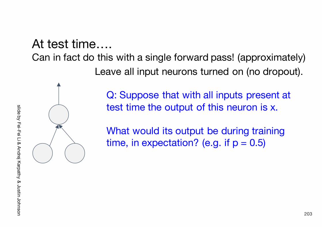
At test time….Can in fact do this with a single forward pass! (approximately)
Leave all input neurons turned on (no dropout).
(this can be shown to be an approximation to evaluating the whole ensemble)
202
slide by Fei-FeiLi & Andrej Karpathy& Justin Johnson
At test time….Can in fact do this with a single forward pass! (approximately)
Leave all input neurons turned on (no dropout).
Q: Suppose that with all inputs present at test time the output of this neuron is x.
What would its output be during training time, in expectation? (e.g. if p = 0.5)
203

slide by Fei-FeiLi & Andrej Karpathy& Justin Johnson
At test time….Can in fact do this with a single forward pass! (approximately)
x y
Leave all input neurons turned on (no dropout).during test: a = w0*x + w1*yduring train:E[a] = ¼ * (w0*0 + w1*0
w0*0 + w1*yw0*x + w1*0
w0*x + w1*y)= ¼ * (2 w0*x + 2 w1*y)
= ½ * (w0*x + w1*y)
a
w0 w1
204

slide by Fei-FeiLi & Andrej Karpathy& Justin Johnson
At test time….Can in fact do this with a single forward pass! (approximately)
x y
Leave all input neurons turned on (no dropout).during test: a = w0*x + w1*yduring train:E[a] = ¼ * (w0*0 + w1*0
w0*0 + w1*yw0*x + w1*0
w0*x + w1*y)= ¼ * (2 w0*x + 2 w1*y)
= ½ * (w0*x + w1*y)
aWith p=0.5, using all inputs in the forward pass would inflate the activations by 2x from what the network was “used to” during training!=> Have to compensate by scaling the activations back down by ½
w0 w1
205

slide by Fei-FeiLi & Andrej Karpathy& Justin Johnson
We can do something approximate analytically
At test time all neurons are active always=> We must scale the activations so that for each neuron:output at test time = expected output at training time
206

slide by Fei-FeiLi & Andrej Karpathy& Justin Johnson
Dropout Summary
drop in forward pass
scale at test time
207

slide by Fei-FeiLi & Andrej Karpathy& Justin Johnson
More common: “Inverted dropout”
test time is unchanged!
208

Summary
• Part 1: Backpropagation and Neural Networks (Basics)
• Part 2: Training Neural Networks (Optimization, Learning tricks)
209
What about the mathematics of deep learning?Why non-convexity does not create a problem in practice?

Local Minima
The Loss Surfaces of Multilayer NetworksA. Choromanska, M. Henaff, M. Mathieu G. B. Arous, Y. LeCun. In AISTATS 2015
Distribution of test losses

Next Lecture: Convolutional Neural Networks
211
![Combining Attributes and Fisher Vectors for Efficient ...erkut/bil722.f12/w11-fadime.pdf · Authors Do Demonstrate that attributes of [1] give excellent results for retrieval Combination](https://static.fdocuments.us/doc/165x107/5ffdcc37c4d1ff323075fc69/combining-attributes-and-fisher-vectors-for-efficient-erkutbil722f12w11-fadimepdf.jpg)