webee.technion.ac.ilwebee.technion.ac.il/Sites/People/DavidMalah/Pubs/FP/Dror-Porat... · THIS...

CONTEXT-BASED MULTIPLE

DESCRIPTION WAVELET IMAGE

CODING

DROR PORAT

CONTEXT-BASED MULTIPLE DESCRIPTION

WAVELET IMAGE CODING

RESEARCH THESIS

SUBMITTED IN PARTIAL FULFILLMENT OF THE

REQUIREMENTS

FOR THE DEGREE OF MASTER OF SCIENCE

IN ELECTRICAL ENGINEERING

DROR PORAT

SUBMITTED TO THE SENATE OF THE TECHNION — ISRAEL INSTITUTE OF TECHNOLOGY

TISHREI, 5770 HAIFA OCTOBER, 2009

THIS RESEARCH THESIS WAS DONE UNDER THE SUPERVISION OF

PROF. DAVID MALAH IN THE DEPARTMENT OF ELECTRICAL

ENGINEERING

ACKNOWLEDGMENT

I would like to express my deep and sincere gratitude to my supervi-

sor, Prof. David Malah, for his excellent professional guidance, steady

support and warm attitude. I would also like to thank Nimrod Peleg

and the rest of the SIPL (Signal and Image Processing Lab) staff for

their continuous technical assistance. I am heartily thankful to my par-

ents, Shmuel and Zehava, for their endless support and encouragement

throughout the way. Last but not least, I wish to thank my loved one

Shira for her unconditional love and support.

THE GENEROUS FINANCIAL HELP OF THE TECHNION IS GRATEFULLY

ACKNOWLEDGED

Contents

Abstract 1

List of Symbols 3

List of Abbreviations 6

1 Introduction 8

1.1 Multiple Description Coding . . . . . . . . . . . . . . . . . . . . . . 8

1.2 Proposed Coding Scheme . . . . . . . . . . . . . . . . . . . . . . . . 10

1.3 Thesis Outline . . . . . . . . . . . . . . . . . . . . . . . . . . . . . . 12

2 Fundamentals of Multiple Description Coding 14

2.1 Introduction to Multiple Description Coding . . . . . . . . . . . . . . 14

2.2 Information Theoretic Aspects . . . . . . . . . . . . . . . . . . . . . 16

2.3 Generation of Multiple Descriptions . . . . . . . . . . . . . . . . . . 24

2.3.1 Progressive Coding and Unequal Error Protection . . . . . . 25

2.3.2 Multiple Description Scalar Quantization . . . . . . . . . . . 26

2.3.3 Multiple Description Correlating Transforms . . . . . . . . . 32

3 Multiple Description Image Coding via Polyphase Transform 39

iii

3.1 System Outline . . . . . . . . . . . . . . . . . . . . . . . . . . . . . . 39

3.2 Experimental Results . . . . . . . . . . . . . . . . . . . . . . . . . . 43

4 Context-Based Multiple Description Wavelet Image Coding:

Motivation and Proposed System Outline 46

4.1 Motivation . . . . . . . . . . . . . . . . . . . . . . . . . . . . . . . . 47

4.1.1 Wavelet Background . . . . . . . . . . . . . . . . . . . . . . . 47

4.1.2 Statistical Characterization of Wavelet Coefficients . . . . . . 50

4.2 Proposed System Outline . . . . . . . . . . . . . . . . . . . . . . . . 58


Context-Based Classification 64

5.1 Introduction . . . . . . . . . . . . . . . . . . . . . . . . . . . . . . . 64

5.2 Classification Rule . . . . . . . . . . . . . . . . . . . . . . . . . . . . 68

5.3 Classification Thresholds Design . . . . . . . . . . . . . . . . . . . . 70


Quantization and Optimal Bit Allocation 77

6.1 Parametric Model-Based Uniform Threshold Quantization . . . . . . 77

6.2 Uniform Reconstruction with Unity Ratio Quantizers as an Alternative

to Uniform Threshold Quantizers . . . . . . . . . . . . . . . . . . . . 84

6.3 Optimal Model-Based Bit Allocation . . . . . . . . . . . . . . . . . . 86


Implementation Considerations and Miscellaneous 94

7.1 Implementation Considerations . . . . . . . . . . . . . . . . . . . . . 94

7.1.1 Boundary Extension for Wavelet Transform . . . . . . . . . . 94

iv

7.1.2 Optimal Bit Allocation for Biorthogonal Wavelet Transform . 98

7.2 Miscellaneous . . . . . . . . . . . . . . . . . . . . . . . . . . . . . . . 101

7.2.1 Prediction Scheme for Approximation Coefficients . . . . . . 101

8 Experimental Results 106

8.1 System Configuration . . . . . . . . . . . . . . . . . . . . . . . . . . 107

8.2 Quality of Classification . . . . . . . . . . . . . . . . . . . . . . . . . 109

8.3 Performance of the System . . . . . . . . . . . . . . . . . . . . . . . 112

8.4 Context Gain . . . . . . . . . . . . . . . . . . . . . . . . . . . . . . . 124

8.5 Determining the Optimal Operating Point Based on Channel Proper-

ties . . . . . . . . . . . . . . . . . . . . . . . . . . . . . . . . . . . . 126

9 Conclusion 130

9.1 Summary . . . . . . . . . . . . . . . . . . . . . . . . . . . . . . . . . 130

9.2 Main Contributions . . . . . . . . . . . . . . . . . . . . . . . . . . . 133

9.3 Future Directions . . . . . . . . . . . . . . . . . . . . . . . . . . . . . 133

A Proof that the Classification Gain G Satisfies G ≥ 1 137

B Reconstruction Offsets of the Optimal Uniform Threshold Quantizer

for the Laplacian Distribution 139

C Proof of a Useful Property of the Laplacian Distribution 141

D Squared Error Distortion of the Optimal Uniform Threshold Quan-

tizer for the Laplacian Distribution 143

E Squared Error Distortion of the Uniform Reconstruction with Unity

v

Ratio Quantizer for the Laplacian Distribution 147

References 149

Hebrew Abstract ��

vi

List of Figures

2.1 Scenario for MD coding with two channels and three receivers. In the

general case there are M channels and 2M − 1 receivers. . . . . . . . . 17

2.2 Side distortion lower bound vs. redundancy ρ for several values of base

rate r. . . . . . . . . . . . . . . . . . . . . . . . . . . . . . . . . . . . 22

2.3 (a) A four-bit uniform scalar quantizer. (b) Two three-bit quantizers

that complement each other so that both outputs together give about

four-bit resolution. (c) More complicated quantizers together attain

four-bit resolution while each having fewer output levels. (From [21]) 27

2.4 Basis configurations for correlating transforms. (a) The standard basis.

(b) Basis for the original correlating transform of [65]. (c) Generaliza-

tion to arbitrary orthogonal bases. (d) Bases that are symmetric with

respect to the principal axis of the source density. (From [24]) . . . . 35

3.1 MD coding system based on polyphase transform and selective quantization. 40

3.2 MD coding system based on polyphase transform and selective quan-

tization for correlated input. . . . . . . . . . . . . . . . . . . . . . . . 42

3.3 Central PSNR vs. side PSNR for image Lena; total rate of 1 bpp. The

polyphase transform-based MD wavelet coder [30] (with two options for

the polyphase transform) is compared with the MDSQ-based coder [46]. 44

vii

4.1 K-level one-dimensional discrete wavelet transform. . . . . . . . . . . 48

4.2 Two-dimensional discrete wavelet transform. Separable filters are first

applied in the horizontal dimension and then in the vertical dimension

to produce a one-level two-dimensional transform. . . . . . . . . . . . 49

4.3 Original image used for demonstrating the two-dimensional wavelet

transform. . . . . . . . . . . . . . . . . . . . . . . . . . . . . . . . . . 51

4.4 Example of a three-level two-dimensional wavelet transform of the orig-

inal image shown in Figure 4.3 (the detail subbands have been en-

hanced to make their underlying structure more visible). . . . . . . . 52

4.5 The generalized Gaussian probability density function of (4.1) with

r = 1 and s = 1.5. . . . . . . . . . . . . . . . . . . . . . . . . . . . . . 54

4.6 Potential conditioning neighbors (also at adjacent scales and orienta-

tions) for a given wavelet coefficient C. . . . . . . . . . . . . . . . . . 56

4.7 MD coding system based on polyphase transform that utilizes context-

based quantization in coding the redundant information. . . . . . . . 59

4.8 Simplified block diagram of the proposed MD encoder. . . . . . . . . 61

4.9 Simplified block diagram of the proposed MD decoder. . . . . . . . . 63

5.1 Context of a given wavelet coefficient Xi,j. The coefficient belongs to

the redundant polyphase component, and is shown in black. The quan-

tized coefficients that form the context belong to the primary polyphase

component, and are shown in white. . . . . . . . . . . . . . . . . . . . 67

5.2 Classification of the coefficient Xi,j based on its activity Ai,j. . . . . . 69

viii

5.3 Merging process performed by the classification thresholds design al-

gorithm. At each iteration, the algorithm merges the pair of classes

with the smallest classification gain among all pairs of adjacent classes. 73

6.1 Uniform threshold quantizer (UTQ) with step size Δ and an odd num-

ber of levels N = 2L + 1. The bin boundaries are denoted by {bj} and

the reconstruction levels by {qj}. The Laplacian pdf is also shown for

illustration. . . . . . . . . . . . . . . . . . . . . . . . . . . . . . . . . 79

6.2 Operational distortion rate function of the optimal UTQ for the unit-

variance Laplacian distribution with squared error distortion. . . . . . 83

6.3 Uniform reconstruction with unity ratio quantizer (URURQ) with step

size Δ and an odd number of levels N = 2L+1. The bin boundaries are

denoted by {bj} and the reconstruction levels by {qj}. The Laplacian

pdf is also shown for illustration. . . . . . . . . . . . . . . . . . . . . 85

7.1 Half-point and whole-point symmetric extensions. (a) Half-point sym-

metric extension. (b) Whole-point symmetric extension. The original

(one-dimensional) input is shown in blue, and the extension is shown

in red. The resulting axes of symmetry are shown in black, and are

located at “half-point” locations in (a) and at “whole-point” locations

in (b). One period of the extended input is shown in solid lines. . . . 96

7.2 Prediction of an approximation coefficient Xi,j based on its quantized

neighbors. The approximation coefficient Xi,j belongs to the redun-

dant polyphase component, and is shown in black. The quantized

coefficients used for the prediction belong to the primary polyphase

component, and are shown in white. . . . . . . . . . . . . . . . . . . . 102

ix

7.3 Quantized coefficients from the primary polyphase component (marked

with asterisks) used to “predict” the value of the quantized approxi-

mation coefficient Xi−1,j−1. . . . . . . . . . . . . . . . . . . . . . . . . 104

8.1 Plain polyphase transform used by the proposed MD coder. . . . . . 108

8.2 Original images (grayscale) of size 512 × 512 pixels.

(a) Lena. (b) Goldhill. . . . . . . . . . . . . . . . . . . . . . . . . . . 110

8.3 (a) Wavelet transform (in absolute value) of the original image Lena,

with approximation coefficients replaced by their corresponding pre-

diction errors. (b) Corresponding classification map (with four gray

levels). . . . . . . . . . . . . . . . . . . . . . . . . . . . . . . . . . . . 111

8.4 Histograms corresponding to the four classes assigned to the coefficients

in subband dH1 of the redundant polyphase component of description 1.

Each histogram also includes a plot of the fitted Laplacian pdf for the

class. . . . . . . . . . . . . . . . . . . . . . . . . . . . . . . . . . . . . 113

8.5 Performance of the proposed MD coder for the image Lena (total rate

of 1 bpp). Also shown is the redundancy rate ρ corresponding to

various points on the performance curve. . . . . . . . . . . . . . . . . 114

8.6 Performance of the proposed MD coder for the image Goldhill (total

rate of 1 bpp). Also shown is the redundancy rate ρ corresponding to

various points on the performance curve. . . . . . . . . . . . . . . . . 115

8.7 Performance of the proposed MD coder (in black), compared to that of

the original polyphase transform-based MD coder [30], utilizing either

the plain polyphase transform or the vector-form polyphase transform

(for the image Lena and a total rate of 1 bpp). . . . . . . . . . . . . . 117

x

8.8 Subjective performance results for the proposed MD coder, also in

comparison to SD coding (for the image Goldhill). (a) Original image

Goldhill. (b) Reconstructed using JPEG2000 (SD) coder (rate 1 bpp).

(c) Central reconstruction by the proposed coder (total rate 1 bpp,

redundancy rate 0.47 bpp). (d) Side reconstruction by the proposed

coder (total rate 1 bpp, redundancy rate 0.47 bpp). . . . . . . . . . . 119

8.9 Subjective performance results for the proposed MD coder, also in

comparison to SD coding (for the image Lena). (a) Original image

Lena. (b) Reconstructed using JPEG2000 (SD) coder (rate 1 bpp).

(c) Central reconstruction by the proposed coder (total rate 1 bpp,

redundancy rate 0.46 bpp). (d) Side reconstruction by the proposed

coder (total rate 1 bpp, redundancy rate 0.46 bpp). . . . . . . . . . . 120

8.10 Performance of the proposed MD coder for various choices of the total

number of classes per subband (for the image Lena and a total rate

of 1 bpp). . . . . . . . . . . . . . . . . . . . . . . . . . . . . . . . . . 121

8.11 Performance of the proposed MD coder, with utilization of URURQs,

compared to utilization of UTQs (for the image Lena and a total rate

of 1 bpp). . . . . . . . . . . . . . . . . . . . . . . . . . . . . . . . . . 123

8.12 Performance of the “no-context coder”, compared to that of the pro-

posed context-based coder in its default configuration (for the image

Lena and a total rate of 1 bpp). Also shown is the redundancy rate ρ

corresponding to various points on the performance curves. . . . . . . 125

8.13 Performance of the proposed MD coder, with the vertical and hori-

zontal axes corresponding to the central distortion and average side

distortion, respectively (for the image Lena and a total rate of 1 bpp). 128

xi

9.1 Polyphase transform-based MD coding system that utilizes context-

based quantization in coding the primary information (reverse context-

based MD coding system). . . . . . . . . . . . . . . . . . . . . . . . . 134

xii

List of Tables

2.1 Index assignment matrix for the quantizer in Figure 2.3(b). The indices

in the left column and top row of the matrix correspond to the red and

blue labels in Figure 2.3(b), respectively. . . . . . . . . . . . . . . . . 29

2.2 Index assignment matrix for the quantizer in Figure 2.3(c). The indices


blue labels in Figure 2.3(c), respectively. . . . . . . . . . . . . . . . . 30

2.3 Index assignment matrix for the quantizer in Figure 2.3(a). The indices


blue labels in Figure 2.3(a), respectively. . . . . . . . . . . . . . . . . 30

7.1 Energy gain factors for the three-level two-dimensional biorthogonal

wavelet transform using Cohen-Daubechies-Feauveau (CDF) 9/7-tap

wavelet filters. . . . . . . . . . . . . . . . . . . . . . . . . . . . . . . . 101

xiii

Abstract

Multiple description (MD) coding is a coding technique that produces several descrip-

tions of a single source of information (e.g., an image), such that various reconstruc-

tion qualities are obtained from different subsets of the descriptions. The purpose of

MD coding is to provide error resilience to information transmitted on lossy networks

(i.e., networks that cannot avoid possible loss of packets). Since there is no hierarchy

of descriptions in MD coding, representations of this type make all of the received

descriptions useful (unlike, for example, layered coding, where a lost layer may also

render other enhancement layers useless). Thus, MD coding is especially suitable for

networks with no priority mechanisms for data delivery, such as the Internet.

Among previous works, MDs for image coding were generated via the utilization of

a decomposition into polyphase-like components (a polyphase transform) and selective

quantization, performed in the wavelet domain. In this research work, we present an

effective way to exploit the special statistical properties of the wavelet decomposition

to provide improved coding efficiency, in the same general framework.

We propose a novel coding scheme that efficiently utilizes contextual information,

extracted from a different polyphase component, to improve the coding efficiency

of each redundant component (aimed to provide an acceptable reconstruction of a

lost polyphase component in the case of a channel failure), and thus enables the

1

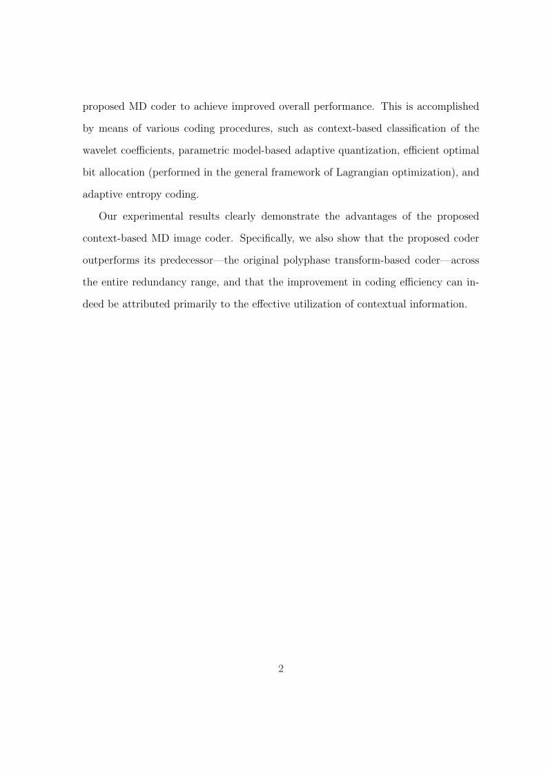
proposed MD coder to achieve improved overall performance. This is accomplished

by means of various coding procedures, such as context-based classification of the

wavelet coefficients, parametric model-based adaptive quantization, efficient optimal

bit allocation (performed in the general framework of Lagrangian optimization), and

adaptive entropy coding.

Our experimental results clearly demonstrate the advantages of the proposed

context-based MD image coder. Specifically, we also show that the proposed coder

outperforms its predecessor—the original polyphase transform-based coder—across

the entire redundancy range, and that the improvement in coding efficiency can in-

deed be attributed primarily to the effective utilization of contextual information.

2

List of Symbols

Ai,j Activity of the wavelet coefficient Xi,j

B Total number of classes from all subbands

Ci,j Context used for classification of the wavelet coefficient Xi,j

C0, . . . , CN Potential classes

D Distortion

Db Distortion in encoding the class b

D′b The derivative of the distortion Db

Dc Central distortion

Di Distortion attained by Decoder i

Ds Average side distortion

D(R) Distortion rate function

D(R) Operational distortion rate function of a quantizer

E [·] Expectation

G Classification gain

Gb Synthesis gain associated with the subband to which class b belongs

Gθ Givens rotation of angle θ

H(·) Entropy

HQ Output entropy of the quantizer Q

3

I(· ; ·) Shannon mutual information

J(·) Lagrangian cost function

L(·) Likelihood function

L∗(·) Log-likelihood function

N Number of pixels in the image

Nb Number of coefficients in the class b

R Rate

Rb Rate for encoding the class b

Ri Transmission rate over Channel i

RT Desired redundancy rate

R(D) Rate distortion function

S Number of subbands

T0, . . . , TN−1 Classification thresholds

Xi,j Wavelet coefficient at the array coordinates (i, j)

X Quantized value of X

{Xk}Nk=1 Sequence of source symbols

{X(i)k }N

k=1 Reconstruction sequence produced by Decoder i

aK Approximation subband (at level K)

{bj} Bin boundaries (of the quantizer)

dHi Horizontal detail subband (at level i)

dVi Vertical detail subband (at level i)

dDi Diagonal detail subband (at level i)

d(·, ·) Distortion measure

{e1, e2} The standard basis of R2

l Index assignment (in MDSQ)

4

{pj} Bin probablities (of the quantizer)

{qj} Reconstruction levels (of the quantizer)

α Initial encoder (in MDSQ)

α0 Encoder (in MDSQ)

β0 Central decoder (in MDSQ)

β1, β2 Side decoders (in MDSQ)

Δ Step size of the quantizer

δ Reconstruction offset

ηb The ratio Nb/N

λ Laplacian parameter

λ Estimated Laplacian parameter

ξ Lagrange multiplier

σ2 Variance

〈·, ·〉 Inner product

5

List of Abbreviations

bpp Bits per pixel

DPCM Differential Pulse Code Modulation

DR Distortion Rate

DWT Discrete Wavelet Transform

ECSQ Entropy-Constrained Scalar Quantization (or Quantizer)

EZW Embedded Zerotree Wavelet (coder)

GGD Generalized Gaussian Distribution

i.i.d. Independent identically distributed

KLT Karhunen-Loeve Transform

MD Multiple Description

MDC Multiple Description Coding

MDLVQ Multiple Description Lattice Vector Quantization (or Quantizer)

MDSQ Multiple Description Scalar Quantization (or Quantizer)

MDVQ Multiple Description Vector Quantization (or Quantizer)

MLE Maximum Likelihood Estimation (or Estimator)

MSE Mean Squared Error

pdf Probability density function

PSNR Peak Signal-to-Noise Ratio

6

RD Rate Distortion

SD Single Description

SI Subsample-Interpolation

SPIHT Set Partitioning In Hierarchical Trees

SQ Scalar Quantization (or Quantizer)

TCP Transmission Control Protocol

UEP Unequal Error Protection

UQ Uniform Quantization (or Quantizer)

URURQ Uniform Reconstruction with Unity Ratio Quantization (or Quantizer)

UTQ Uniform Threshold Quantization (or Quantizer)

VQ Vector Quantization (or Quantizer)

7

Chapter 1

Introduction

1.1 Multiple Description Coding

Multiple description (MD) coding is a coding technique that represents a single source

of information (e.g., an image) with several chunks of data, called descriptions, in

such a way that the source can be approximated from any (non-empty) subset of the

descriptions. The purpose of MD coding is to provide error resilience to information

transmitted on lossy networks, such as the Internet, where inevitable loss of data may

severely degrade the performance of conventional coding techniques. For example,

in layered coding, where the information is represented hierarchically, a lost layer

may also render other enhancement layers useless. MD coding, on the other hand,

makes all of the received descriptions useful, and thus can better mitigate transport

failures. It is clear that in order to gain robustness to the possible loss of descriptions,

some compression efficiency must be sacrificed (i.e., the representation is redundant).

That is the reason why MD coding should be applied only if this disadvantage in

compression efficiency is offset by the advantage of mitigating transport failures.

8

Many MD coding schemes focus on the case of two descriptions, mainly due to its

relative tractability, and so does this work. The basic situation of MD coding, for the

two-description case, is as follows [15]: Suppose that we wish to send a description

of an information source over an unreliable communication network, namely, one

with nonzero probability for the event of description loss. In order to deal with

the possibility of a lost description, or due to constraints imposed by the network

regarding the size of packets, we decide to send two descriptions instead and hope

that at least one of them will get through. Obviously, each description should be

individually good due to the possibility that only one description will get to the

destination. However, in the case that both descriptions get through, we wish to

maximize the combined descriptive information at the receiver.

Among prior works, MDs for image coding were generated via the utilization of a

decomposition into polyphase-like components (a polyphase transform) and selective

quantization [30], performed in the wavelet domain. Unlike many other MD coding

techniques, such as MD scalar quantization [59] and MD correlating transforms [65],

the technique of MD coding via polyphase transform and selective quantization ex-

plicitly separates description generation and redundancy addition, which significantly

reduces the complexity of the system design and implementation. This technique also

enables to easily generate descriptions of statistically equal rate and importance, a

property which is well suited to communication systems with no priority mechanisms

for data delivery (e.g., the Internet).

For description generation, in the two-description case discussed herein, the afore-

mentioned technique employs a polyphase transform, and each of the two resulting

polyphase components is coded independently at a source coding rate to constitute

9

the primary part of information for its corresponding description. In order to ex-

plicitly add redundancy to each description, the other polyphase component is then

coded at a (usually lower) redundancy coding rate using selective quantization and

added to this description. In case of a channel failure, this redundancy enables an

acceptable reconstruction of the lost component.

1.2 Proposed Coding Scheme

In this research work, we develop and explore an effective way to exploit the spe-

cial statistical properties of the wavelet decomposition to provide improved coding

efficiency, in the general framework of polyphase transform-based MD image coding.

We propose a novel coding scheme that efficiently utilizes contextual information,

extracted from the primary polyphase component of each description, to improve

the coding efficiency of the corresponding redundant polyphase component, and thus

enables the proposed MD coder to achieve improved overall performance. This is

accomplished by means of various coding procedures, such as context-based classi-

fication of the wavelet coefficients, parametric model-based adaptive quantization,

efficient optimal bit allocation, and adaptive entropy coding.

In order to efficiently utilize the statistical dependencies between neighboring

wavelet coefficients, and avoid the need for an explicit characterization of these de-

pendencies, we use an effective context-based classification procedure. To avoid the

penalty of forward classification, the classification is based on contexts formed from

quantized coefficients of the primary polyphase component of the description, which

are also available at the decoder, and thus no transmission of side information is

required. Nevertheless, a controlled amount of side information is still produced and

10

transmitted to the decoder, in order to improve the performance of the system. This

side information includes the classification thresholds, allowing to select a class for a

coefficient given its context, as well as the source statistics of each class, where each

class is modeled using a parametric Laplacian distribution. The parametric modeling

is also utilized by the bit allocation, quantization and entropy coding procedures that

follow.

The context-based classification procedure enables the proposed coder to utilize a

set of quantizers, each customized to an individual class. For this task, we examine two

types of quantizers: the uniform threshold quantizer (UTQ) and the uniform recon-

struction with unity ratio quantier (URURQ). Both of these quantizers well approx-

imate the optimum entropy-constrained scalar quantizer (ECSQ) for the Laplacian

distribution, assuming mean squared error (MSE) distortion, and are relatively simple

to design and operate. In order to avoid the high complexity of entropy-constrained

design algorithms for the quantizers, we propose an efficient design strategy, that is

based on a pre-designed indexed array of MSE-optimized quantizers of different step

sizes for the Laplacian distribution. To further reduce the complexity of the proposed

design strategy, we also derive closed form expressions for the distortions attained by

both the UTQ and the URURQ.

For bit allocation between the various classes in the different subbands, we develop

an optimal and efficient model-based bit allocation scheme, in the general framework

of Lagrangian optimization, which also takes into account the non-energy preserving

nature of the biorthogonal wavelet transform. Our bit allocation scheme, which is

based on variance scaling and on the aforementioned pre-designed indexed array of

MSE-optimized quantizers, enables the proposed coder to avoid complex on-line bit

allocation procedures, as well as to intelligently and instantly adapt the arithmetic

11

entropy encoder to the varying coefficients statistics.

Finally, we also suggest a way to determine, in practice, the optimal operating

point for the proposed MD coder, based on the properties of the communication

channel.

1.3 Thesis Outline

This thesis is organized as follows. Chapter 2 introduces the MD scenario, summarizes

the main results in the theory of MD coding, and provides an overview of some existing

MD coding techniques. Chapter 3 provides a detailed review of an efficient technique

for MD image coding utilizing a polyphase transform and selective quantization, which

forms the framework of our proposed context-based MD coding system. Chapter 4

provides the motivation for context-based MD coding in the wavelet domain, and also

presents the outline of the proposed context-based MD wavelet image coder. A more

detailed description of the main building blocks of the proposed coder is provided in

the subsequent chapters.

In Chapter 5 we describe the context-based classification procedure, which en-

ables the proposed coder to use a set of customized quantizers for improved coding

efficiency. Chapter 6 provides a detailed description of the parametric model-based

quantization and bit allocation schemes. In Chapter 7 we comprehensively address

some implementation considerations, which are also generally related to efficient im-

plementation of wavelet coders, including boundary extensions for the wavelet trans-

form (especially referring to coding applications), and optimal bit allocation for the

biorthogonal wavelet transform.

12

Chapter 8 provides exhaustive experimental results, which also include a compar-

ison to other relevant MD image coding systems. It also provides a way to optimally

determine, in practice, the operating point for the proposed coder, based on the

properties of the communication channel.

Finally, Chapter 9 concludes this thesis and describes several possible directions

for future research.

13

Chapter 2

Fundamentals of Multiple

Description Coding

This chapter introduces the MD scenario, summarizes the main results in the theory

of MD coding, and provides an overview of some existing MD coding techniques.

2.1 Introduction to Multiple Description Coding

As described in Section 1.1, the basic problem that multiple description coding deals

with is how to represent a single source of information with several chunks of data

(“descriptions”) in such a way that the source can be approximated from any subset

of the chunks [21].

Current systems that deliver content over packet networks typically generate

the transmitted data with a progressive coder and use TCP (Transmission Control

Protocol)—the standard protocol that controls retransmission of lost packets—in or-

der to deliver the data over the network. The main drawback of such techniques is

14

that the order in which packets are received is critical, which may cause intolerable

delays when packets are lost. For example, suppose that an image is compressed

using a progressive (layered) coder that generates L packets, numbered from 1 to L.

The receiver reconstructs the image from the received packets and the quality of the

reconstructed image is improved steadily as the number of consecutive packets re-

ceived, starting from the first, increases. If the first two packets are received but the

third packet, for instance, is not, the quality of the reconstructed image is propor-

tionate to reception of only two packets, no matter how many of the other packets

are received. Receiving the third packet may require retransmission of that packet,

which introduces a delay. Such delays may be much longer than the inter-arrival

times between received packets and therefore hurt the performance of the system.

The above example shows that although progressive transmission works well when

packets are received in order without loss, the performance of such a system may be

degraded when packet losses occur.

In a constellation where losses are inevitable, it would be highly beneficial to create

representations that make all of the received packets useful, not just those consecutive

from the first. The purpose of MD coding is to create such representations. It

is clear that in order to gain robustness to the possible loss of descriptions, some

compression efficiency must be sacrificed. That is the reason why MD coding should

be applied only if this disadvantage in compression efficiency is offset by the advantage

of mitigating transport failures.

In the remainder of this chapter, unless specified otherwise, we focus on the two-

description case for the sake of conciseness and clarity. Nevertheless, many of the

ideas and results presented in the sequel can be extended to the case of more than

two descriptions.

15

The basic situation of MD coding, for the two-description case, is as follows [15]:

Suppose that we wish to send a description of a random process (information source)

over an unreliable communication network—one with nonzero probability for the

event of description loss. In order to deal with the possibility of a lost description, or

due to constraints imposed by the network regarding the size of packets, we decide

to send two descriptions instead and hope that at least one of them will get through.

Obviously, each description should be individually good due to the possibility that

only one description will get to the destination. However, in the case that both

descriptions get through, we wish to maximize the combined descriptive information

at the receiver.

The difficulty in generation of such descriptions is that good individual descrip-

tions must be close to the process (by virtue of their goodness) and therefore must

be highly dependent. Such a dependency implies that the second description will

contribute only little extra information beyond one description alone. On the other

hand, two descriptions that are independent from each other must be far apart and

therefore cannot in general be individually good. Essentially, this demonstrates the

fundamental tradeoff of MD coding: creating descriptions that are individually good

and yet not too similar.

2.2 Information Theoretic Aspects

The following is known as the MD problem: if an information source is described

with two separate descriptions, what are the concurrent limitations on the qualities

of these descriptions taken separately and jointly?

The MD situation for the two-description case is shown schematically in Figure 2.1.

16

A sequence of source symbols {Xk}Nk=1 is encoded and transmitted to three receivers

Source Encoder Decoder 0

Decoder 1

Decoder 2

Channel 1

Channel 2

(1)ˆk

X

kX{ }

{ }

(0)ˆk

X{ }

(2)ˆk

X{ }

Figure 2.1: Scenario for MD coding with two channels and three receivers. In thegeneral case there are M channels and 2M − 1 receivers.

over two noiseless (or error corrected) channels. One decoder, called the central

decoder, receives information from both channels, while the other two decoders, called

the side decoders, receive information only from their respective channels. We denote

the transmission rate over Channel i by Ri, i = 1, 2, in bits per source sample.

The reconstruction sequence produced by Decoder i is denoted by {X(i)k }N

k=1 with

respective distortion

Di =1

N

N∑k=1

E[d(Xk, X

(i)k

)], i = 0, 1, 2 (2.1)

where d(·, ·) is a nonnegative, real-valued distortion measure1.

It should be noted that the situation drawn in Figure 2.1 of three separate users

or three classes of users (applicable to broadcasting over two channels, for example)

can also serve as an abstraction to the case of a single user that can be in one of three

1Actually, a different distortion measure may be used for each of the reconstructed sequences. Asingle distortion measure is assumed here for simplicity.

17

states depending on which descriptions are received. We will usually adopt the latter

interpretation.

Several interesting problems in rate distortion theory are introduced by the MD

model. The central theoretical problem is the following [21]: given an information

source and a distortion measure, determine the set of achievable values for the quin-

tuple (R1, R2, D0, D1, D2). These theoretical bounds are of major importance and are

discussed next.

Recall the definition of the rate distortion region in the one-description rate dis-

tortion problem: for a given source and distortion measure, the rate distortion (RD)

region is the closure of the set of achievable rate distortion pairs (where a rate dis-

tortion pair (R, D) is called achievable if, for some positive integer n, there exists a

source code with length n, rate R and distortion D). As an extension, the MD rate

distortion region, or simply MD region is defined, for a given source and distortion

measure, as the closure of the set of simultaneously achievable2 rates and distortions

in MD coding. Specifically, for the two-description case, the MD region is the closure

of the set of achievable quintuples (R1, R2, D0, D1, D2).

Unfortunately, unlike RD regions in the one-description rate distortion prob-

lem [48], MD regions have not been completely characterized in terms of single-letter

information theoretic quantities (entropy, mutual information, etc.). The following

theorem of El Gamal and Cover [15] shows how achievable quintuples can be deter-

mined from joint distributions of source and reproduction random variables.

Theorem 2.1 [15] Let X1, X2, . . . be a sequence of i.i.d. finite alphabet3 random

2The meaning of “achievable” in this context is the immediate extension from the one-descriptionrate distortion problem.

3Although the proof of the theorem assumes a finite alphabet, it can be extended to the Gaussiansource, as noted in [15].

18

variables drawn according to a probability mass function p(x). Let d(·, ·) be a bounded

distortion measure. An achievable rate region for distortion D = (D1, D2, D0) is given

by the convex hull of all (R1, R2) such that

R1 > I(X; X(1)) (2.2)

R2 > I(X; X(2)) (2.3)

R1 + R2 > I(X; X(0), X(1), X(2)) + I(X(1); X(2)) (2.4)

for some probability mass function p(x, x(0), x(1), x(2)) = p(x)p(x(0), x(1), x(2)|x) such

that

D1 ≥ E[d(X, X(1))

](2.5)

D2 ≥ E[d(X, X(2))

](2.6)

D0 ≥ E[d(X, X(0))

](2.7)

and where I(· ; ·) denotes Shannon mutual information [13].

It should be noted that Theorem 2.1 does not specify all achievable quintuples, un-

fortunately. The points that can be obtained in this manner are therefore called inner

bounds to the MD region. Other characterizations of achievable points in terms of

information theoretic quantities for the two-description case [68] and for more than

two descriptions [63] also generally do not give the entire MD region.

Points that are certainly not in the MD region are called outer bounds. Rate

distortion functions provide the simplest outer bounds: In order to have distortion

D1, Decoder 1 must receive at least R(D1) bits per symbol, where R(D) is the rate

distortion function of the source (with the given distortion measure). By making

19

similar arguments for the other two decoders we get the bounds

R1 + R2 ≥ R(D0) (2.8)

Ri ≥ R(Di), i = 1, 2. (2.9)

The bounds (2.8) and (2.9) are usually loose due to the difficulty in making the

individual and joint descriptions good.

Memoryless Gaussian sources and the squared error distortion measure4 are of

special importance (also) in MD coding. First, this is the only case for which the

MD region is completely known. Ozarow showed in [41] that for this source and

distortion measure, the MD region is exactly the largest set that can be obtained

with the achievable region of El Gamal and Cover. Moreover, the MD region for any

continuous-valued memoryless source with squared error distortion measure can be

bounded using the MD region for Gaussian sources [67]. Useful intuition and insight

into the limitations in MD coding can be gained from this special case and so we now

turn to a more detailed analysis of it.

For a memoryless Gaussian source with variance σ2 and squared error distortion

measure, the MD region consists of (R1, R2, D0, D1, D2) that satisfy [21]

Di ≥ σ22−2Ri , i = 1, 2 (2.10)

D0 ≥ σ22−2(R1+R2) · γD (2.11)

where γD = 1 if D1 + D2 > σ2 + D0, and

γD =1

1 −(√

(1 − D1)(1 − D2) −√

D1D2 − 2−2(R1+R2))2 (2.12)

otherwise (obviously γD ≥ 1 from (2.11) and the fact that D(R) = σ22−2R is the

distortion rate function for a Gaussian source with squared error distortion). The

4The squared error distortion measure is given by d(x, x) = (x − x)2.

20

relation (2.11) is pivotal as it indicates that there is a multiplicative factor γD by

which the central distortion must exceed the distortion rate minimum. When at least

one of the side distortions is sufficiently large, γD = 1 and the central reconstruction

can be very good. Otherwise, there is a penalty in the central distortion, determined

by the value of γD from (2.12).

In the special case that R1 = R2 and D1 = D2, called the balanced case in the

terminology of MD coding, the following side distortion bound for a source with unit

variance can be proved to hold [20] (in addition to the bound D1 ≥ σ22−2R1):

D1 ≥ min

{1

2

[1 + D0 − (1 − D0)

√1 − 2−2(R1+R2)/D0

], 1 −

√1 − 2−2(R1+R2)/D0

}.

(2.13)

Introducing the total rate R1 + R2 as the sum of a base rate r = R(D0) and a

redundancy ρ = R1 + R2 − R(D0) gives the alternative formulation

D1 ≥

⎧⎪⎨⎪⎩

12

[1 + 2−2r − (1 − 2−2r)

√1 − 2−2ρ

], for ρ ≤ r − 1 + log2(1 + 2−2r)

1 −√1 − 2−2ρ , for ρ > r − 1 + log2(1 + 2−2r).

(2.14)

This bound is plotted in Figure 2.2 as a function of the redundancy ρ for several

values of the base rate r (in bits/sample).

It is instructive to examine the behavior of the bound (2.14) in the low redundancy

region. In this region, the partial derivative of the side distortion lower bound with

respect to ρ is given by

∂D1

∂ρ= −(1 − 2−2r) ln 2

2· 2−2ρ

√1 − 2−2ρ

(2.15)

and for any fixed r > 0 we get

limρ→0+

∂D1

∂ρ= −∞. (2.16)

21

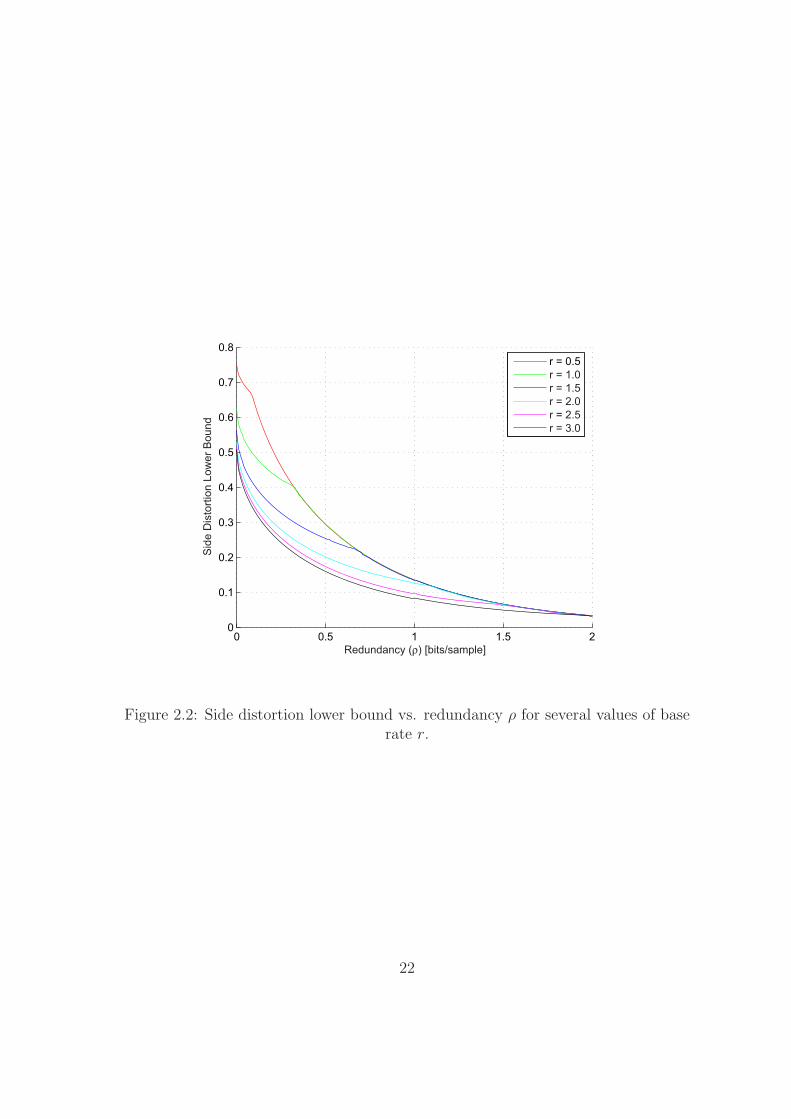
0 0.5 1 1.5 20

0.1

0.2

0.3

0.4

0.5

0.6

0.7

0.8

Redundancy (ρ) [bits/sample]

Sid

e D

isto

rtion

Low

er B

ound

r = 0.5r = 1.0r = 1.5r = 2.0r = 2.5r = 3.0

Figure 2.2: Side distortion lower bound vs. redundancy ρ for several values of baserate r.

22

For an interpretation of this result, consider an MD coding system that achieves the

rate distortion bound for the central decoder. If a small additional increase in rate

is allowed, what would be an intelligent way to spend it? A common performance

measure in MD coding systems is some linear combination of central and side dis-

tortions (in which the weights usually correspond to probabilities of receiving certain

combinations of descriptions). In such a case, the infinite slope at ρ = 0+ implies that

it will be much more efficient to dedicate the small additional rate to reducing the

side distortion rather than to reducing the central distortion. Essentially, a nonzero

redundancy should ideally be used by such a system.

The significant effect of a small amount of redundancy in MD coding systems is

observed even when actual performance is considered, not merely bounds. For exam-

ple, in the MD coding technique of correlating transforms (discussed in Section 2.3.3),

an infinite side distortion slope is again observed at zero redundancy [23, 24].

Ozarow’s result is often interpreted as an exponential lower bound on the product

of central and side distortions. Assuming that R1 = R2 � 1 and D1 = D2 ≈2−2(1−ν)R1 with 0 < ν ≤ 1, γD can be estimated as (4D1)

−1. The bound in (2.11)

then gets the form

D0 · D1 ≥ σ2

42−4R1 (2.17)

which explains the reason for this interpretation of Ozarow’s result. This optimal rate

of exponential decay of the product of central and side distortions can be attained by

MD quantization techniques [59, 60] (MD quantization is discussed in Section 2.3.2).

23

2.3 Generation of Multiple Descriptions

This section provides a concise description of some common MD coding techniques.

Powerful MD codes can be built from combination of MD coding techniques, like MD

quantizers and transforms [21], along with channel codes and basic components of

modern compression systems, such as prediction, scalar quantization, decorrelating

transforms and entropy coding [22].

One of the simplest ways to produce multiple descriptions is to partition the

source data into several parts and then compress each part independently to produce

the descriptions. Proper interpolation can be used to decode from any (non-empty)

subset of the descriptions. For example, one can separate a speech signal into odd- and

even-numbered samples to produce two descriptions, encode them independently and

employ one-dimensional interpolation upon decoding if one of the descriptions is lost,

as in Jayant’s subsample-interpolation (SI) approach [28, 29]. This separation can also

be adapted to multidimensional data, such as images [52]. Although this technique

can be very powerful, it has a serious drawback, as it relies completely on the existence

and amount of redundancy already present in the source (in the form of correlation or

memory). Additionally, in order to be complementary to modern compression systems

that initially reduce correlation by means of prediction or decorrelating transforms,

an MD coding technique must work well on memoryless sources. We now turn to

describe such techniques in detail.

24

2.3.1 Progressive Coding and Unequal Error Protection

Generation of two descriptions can be easily performed by duplication of a single

description of the source. This description can be produced with the best (single-

description) compression technique available. If only one description is received, the

performance is the best possible in such a case. Nevertheless, receiving both descrip-

tions provides no further improvement in performance.

A more flexible and controllable approach is to repeat only some fraction of the

data. Ideally, the repeated data would be the most important, and thus this type of

fractional repetition is naturally matched to progressive source coding. In order to

produce two R-bit descriptions, first set ζ ∈ [0, 1] and encode the source to a rate

(2−ζ)R with a progressive source code. The first ζR bits are the most important and

thus are repeated in both descriptions, while the remaining (2−ζ)R−ζR = 2(1−ζ)R

bits are split between the descriptions (in a meaningful way). Essentially, this strategy

protects some of the bits with a rate-1/2 channel code5 (repetition), while the other

bits are left unprotected. It is therefore called an unequal error protection (UEP)

strategy for MD coding. UEP can also be easily generalized to the case of more than

two descriptions.

When designing an MD coding system based on UEP, one has to determine the

amount of data to be coded at each channel code rate. Techniques for this assignment

that are based on optimization of a scalar objective function are described in [38, 43].

In order to assess the performance of UEP as an MD coding technique, the MD

rate distortion region (defined in Section 2.2) can be compared to the corresponding

5A block channel code that maps k input symbols to n output symbols, with n > k, is said tohave rate k/n.

25

region attained with UEP. Both regions can be determined completely for the two-

description case with memoryless Gaussian source and squared error distortion mea-

sure. Comparing the minimum attainable central distortions for fixed values of side

distortions can be used to characterize the difference between these regions. The max-

imum gap in central distortion over all rates and side distortions is about 4.18 dB [20].

Although bounded, this gap is quite significant, and analogous comparisons show that

it increases for more descriptions [63].

2.3.2 Multiple Description Scalar Quantization

We begin this section with a description of a natural way to use scalar quantizers

to create multiple descriptions for communication over two channels—a purpose also

known in this context as channel splitting due to its origin. We later introduce a

more systematic and efficient approach to construct scalar quantizer pairs known as

multiple description scalar quantization (MDSQ).

We start with an example demonstrating the difficulty in creating two useful

descriptions of a source without added redundancy. Consider trying to communicate,

using 4 bits, a single real number x ∈ [−1, 1]. One option, which is optimal if the

source is uniformly distributed, is the four-bit uniform scalar quantizer shown in

Figure 2.3(a) with black labels. There is no satisfactory way to split the four bits

into two pairs for transmission over two channels since any reconstruction by the side

decoder that does not receive the most significant bit (MSB) will, on average, be

poor. One reasonable labeling under these circumstances is shown in Figure 2.3(a)

with red and blue labels, but even this does not produce good estimates in a consistent

manner.

A natural way to use scalar quantizers for channel splitting is to combine two

26

Figure 2.3: (a) A four-bit uniform scalar quantizer. (b) Two three-bit quantizersthat complement each other so that both outputs together give about four-bit

resolution. (c) More complicated quantizers together attain four-bit resolution whileeach having fewer output levels. (From [21])

uniform quantizers (one for each channel) with an offset between them, as shown in

Figure 2.3(b) in red and blue. Due to this offset, combining the information from

both channels gives one additional bit of resolution. To avoid clutter, we do not show

the reconstructions computed when both channels are available; as an example, if

q1(x) = 110 and q2(x) = 101, then x must be in the interval [7/16, 9/16) and thus is

reconstructed to 1/2.

Indeed, the quantizers in Figure 2.3(b) produce good side reconstructions (i.e.,

the reconstructions from either channel alone are good), but this comes at the cost

of a fairly high redundancy: the total rate over both channels is 6 bits/sample, while

the reconstruction quality when both channels are received is comparable to that

of the 4-bit quantizer in Figure 2.3(a). More generally, using two B-bit quantizers

(offset from each other) to create the descriptions produces approximately (B + 1)-

bit resolution for the central decoder, while the total rate is 2B bits/sample. Due to

the high redundancy, this solution is usually unsatisfactory (at least unless the side

27

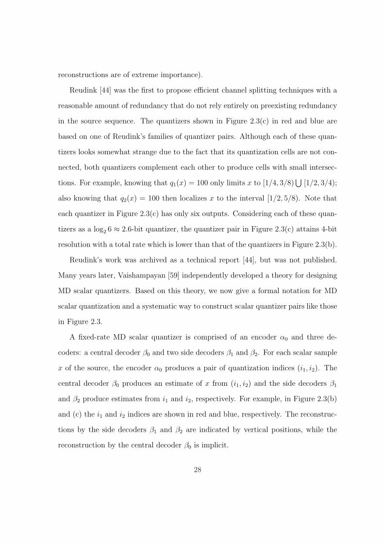
reconstructions are of extreme importance).

Reudink [44] was the first to propose efficient channel splitting techniques with a

reasonable amount of redundancy that do not rely entirely on preexisting redundancy

in the source sequence. The quantizers shown in Figure 2.3(c) in red and blue are

based on one of Reudink’s families of quantizer pairs. Although each of these quan-

tizers looks somewhat strange due to the fact that its quantization cells are not con-

nected, both quantizers complement each other to produce cells with small intersec-

tions. For example, knowing that q1(x) = 100 only limits x to [1/4, 3/8)⋃

[1/2, 3/4);

also knowing that q2(x) = 100 then localizes x to the interval [1/2, 5/8). Note that

each quantizer in Figure 2.3(c) has only six outputs. Considering each of these quan-

tizers as a log2 6 ≈ 2.6-bit quantizer, the quantizer pair in Figure 2.3(c) attains 4-bit

resolution with a total rate which is lower than that of the quantizers in Figure 2.3(b).

Reudink’s work was archived as a technical report [44], but was not published.

Many years later, Vaishampayan [59] independently developed a theory for designing

MD scalar quantizers. Based on this theory, we now give a formal notation for MD

scalar quantization and a systematic way to construct scalar quantizer pairs like those

in Figure 2.3.

A fixed-rate MD scalar quantizer is comprised of an encoder α0 and three de-

coders: a central decoder β0 and two side decoders β1 and β2. For each scalar sample

x of the source, the encoder α0 produces a pair of quantization indices (i1, i2). The

central decoder β0 produces an estimate of x from (i1, i2) and the side decoders β1

and β2 produce estimates from i1 and i2, respectively. For example, in Figure 2.3(b)

and (c) the i1 and i2 indices are shown in red and blue, respectively. The reconstruc-

tions by the side decoders β1 and β2 are indicated by vertical positions, while the

reconstruction by the central decoder β0 is implicit.

28

Vaishampayan [59] proposed a useful visualization technique for the encoding op-

eration. First, the encoding operation α0 is presented as α0 = l ◦ α—the composition

of an index assignment l and an initial encoder α. The initial encoder α is an ordinary

quantizer, i.e., it partitions the real line into cells that are intervals. The index as-

signment l, which must be invertible, produces a pair of indices (i1, i2) from the single

index produced by the ordinary quantizer α. Vaishampayan’s visualization technique

is to write out l−1, forming the index assignment matrix.

The index assignment matrix corresponding to the quantizer in Figure 2.3(b) is

shown in Table 2.1, where the cells of the initial encoder α, taken in increasing values

of x, are numbered from 0 to 14. The redundancy in the representation by this

000 001 010 011 100 101 110 111000 0001 1 2010 3 4011 5 6100 7 8101 9 10110 11 12111 13 14

Table 2.1: Index assignment matrix for the quantizer in Figure 2.3(b). The indicesin the left column and top row of the matrix correspond to the red and blue labels

in Figure 2.3(b), respectively.

quantizer is indicated by the fact that the corresponding index assignment matrix

has only 15 out of 64 cells occupied. The qualities of the side reconstructions are

indicated by the relatively small range of values in any row or column of the matrix

(a maximum difference of 1).

Lower redundancy can be achieved using an index assignment matrix with a higher

29

fraction of occupied cells. Table 2.2 shows the index assignment matrix for the quan-

tizer in Figure 2.3(c). A higher fraction of occupied cells (16 out of 36) in this example

000 001 010 011 100 101000 0 1001 2 3 5010 4 6 7011 8 9 11100 10 12 13101 14 15

Table 2.2: Index assignment matrix for the quantizer in Figure 2.3(c). The indicesin the left column and top row of the matrix correspond to the red and blue labels

in Figure 2.3(c), respectively.

indicates lower redundancy, but the extended range of values in any row or column

of the index assignment matrix (a maximum difference of 3) implies that the side

distortions are higher.

If all the cells of the index assignment matrix are occupied, there is no redundancy.

However, the side distortions in this case are necessarily high. For a four-bit quantizer

α and zero redundancy, Table 2.3 shows the best possible index assignment, as also

marked in Figure 2.3(a) with red and blue labels.

00 01 10 1100 0 1 5 601 2 4 7 1210 3 8 11 1311 9 10 14 15

Table 2.3: Index assignment matrix for the quantizer in Figure 2.3(a). The indicesin the left column and top row of the matrix correspond to the red and blue labels

in Figure 2.3(a), respectively.

30

In the design of an MD scalar quantizer, the optimization of the ordinary quan-

tizer α and the decoders β0, β1 and β2 is relatively easy. The optimization of the

index assignment l is very difficult, however. Instead of addressing the exact optimal

index assignment problem, Vaishampayan [59] gave several heuristic guidelines that

are likely to give performance which is close to the best possible. Essentially, the cells

of the index assignment matrix should be filled from the upper-left to the lower-right

and from the main diagonal outward, as demonstrated in the examples above.

The theory of designing MD scalar quantizers is extended from fixed-rate quanti-

zation to entropy-constrained quantization in [61].

The design of an MD scalar quantizer offers convenient adaptation of the quantizer

according to the relative importance of the central distortion and each side distor-

tion. For the balanced case, where R1 = R2 and D1 = D2, and assuming high rates,

the central and side distortions can be traded off while keeping their product con-

stant [59, 61]. In addition, it can be shown that the exponential decay of this product

as a function of the rate matches the optimal decay implied by [41], while the lead-

ing constant terms are consistent with what one would expect from high-resolution

analysis of ordinary (single description) scalar quantizers [60].

The formalism of MD scalar quantization can be extended to MD vector quantiza-

tion (MDVQ), but the actual quantizer design and encoding may become impractical

if no additional constraints are placed. This is because the complexity of the initial

quantization mapping α increases exponentially with the vector’s dimension N and

because the heuristic guidelines for the design of the index assignment l in MDSQ do

not extend to MDVQ as there is no natural order on RN . These difficulties are avoided

by the elegant technique of MD lattice vector quantization (MDLVQ) of Servetto et

al. [47, 62], where the index assignment problem is simplified by lattice symmetries

31

and the complexity is reduced due to the structure of the lattice [12]. Other related

MD quantization techniques are described in [17, 18, 26].

Obviously, MD scalar quantization can also be applied to transform coefficients.

For the case of high rates, it is shown in [3] that the transform optimization problem

is essentially unchanged from conventional (single description) transform coding. The

technique of MD correlating transforms described next also utilizes transforms and

scalar quantizers, but, in contrast to MD scalar quantization, gets its MD character

from the transform itself.

2.3.3 Multiple Description Correlating Transforms

This section provides a concise description of a useful technique for meeting MD

coding objectives in the framework of standard transform-based coding through the

design of correlating transforms [24]. The basic idea in standard transform coding is to

eliminate statistical dependency and produce uncorrelated transform coefficients [22].

In the scenario of MD coding, however, statistical dependency between transform co-

efficients may prove useful as it can improve the estimation of transform coefficients

that are in a lost description. The technique of MD coding using correlating trans-

forms, proposed by Wang et al. [65], is based on explicit introduction of correlation

between pairs of random variables through a linear transform (called a correlating

transform in this context due to its purpose).

Relating to the two-description case, let X1 and X2 be statistically independent

zero-mean Gaussian random variables with variances σ21 > σ2

2. In the case of con-

ventional (single description) source coding, there would be no reason to use a linear

transform prior to quantization. For a rate R (in bits per sample) and assuming high-

rate entropy-coded uniform quantization, the MSE distortion per component would

32

be given by [22]

D0 =πe

6σ1σ22

−2R, (2.18)

which is the best possible performance in this case.

In the two-description MD scenario, suppose that the quantized versions of X1

and X2 are sent on channels 1 and 2, respectively. Due to the statistical independence

of X1 and X2, side decoder 1 cannot do better than estimating X2 using its mean.

Therefore

D1 =πe

12σ1σ22

−2R +1

2σ2

2 (2.19)

and, similarly,

D2 =πe

12σ1σ22

−2R +1

2σ2

1. (2.20)

Under the assumption that each channel is equally likely to fail, instead of considering

D1 and D2 separately, it is reasonable to consider the average distortion when one

description is lost

D1 =1

2(D1 + D2) =

1

4(σ2

1 + σ22) +

πe

12σ1σ22

−2R. (2.21)

The average side distortion D1 could be reduced if side decoder i had some in-

formation about Xj, j �= i. This can be achieved by sending correlated transform

coefficients instead of the Xi’s themselves, i.e., to send quantized versions of Y1 and

Y2 given by ⎡⎢⎣ Y1

Y2

⎤⎥⎦ =

⎡⎢⎣ a b

c d

⎤⎥⎦⎡⎢⎣ X1

X2

⎤⎥⎦ . (2.22)

Specifically, let us consider the original transform proposed in [65], where⎡⎢⎣ Y1

Y2

⎤⎥⎦ =

1√2

⎡⎢⎣ 1 1

1 −1

⎤⎥⎦⎡⎢⎣ X1

X2

⎤⎥⎦ . (2.23)

33

Since [Y1, Y2]T is obtained using an orthonormal transformation and MSE distortion

is considered, the distortion in approximating the Xi’s equals the distortion in ap-

proximating the Yi’s. Since the variance of both Y1 and Y2 is (σ21 + σ2

2)/2, the central

distortion is given by

D0 =πe

6

(σ2

1 + σ22

2

)2−2R, (2.24)

which is worse than the performance attained without using the correlating transform

by a constant factor of

Γ =(σ2

1 + σ22)/2

σ1σ2

. (2.25)

Note that Γ ≥ 1 as the ratio of an arithmetic and a geometric mean, and that σ21 > σ2

2

implies Γ > 1.

For each side decoder, the total distortion is approximately equal to the quantiza-

tion error plus the distortion in estimating the missing coefficient from the received

one. Using the fact that Y1 and Y2 are jointly Gaussian, it can be shown that [24]

D1 ≈ σ21σ

22

σ21 + σ2

2

+πe

12

(σ2

1 + σ22

2

)2−2R. (2.26)

By comparing (2.21) and (2.26), one can see that the use of the transform given

by (2.23) reduced the constant term in D1 by the factor Γ2, while the exponential

term was increased by the factor Γ. Along with (2.18) and (2.24), this shows that

the technique of correlating transforms enables the central and side distortions to be

traded off. Intermediate tradeoffs can be obtained by using other orthogonal trans-

forms. As also discussed later in this section, additional operating points, including

more extreme tradeoffs, can be attained by using nonorthogonal transforms [39]. Note

that the factor Γ approaches unity as σ1/σ2 → 1; thus, the pairwise correlation has

no effect when the joint density of X1 and X2 has spherical symmetry (this fact holds

equally well for both orthogonal and nonorthogonal transforms).

34

We now give a useful geometric interpretation to the use of correlating transforms

for MD coding. As before, let X = [X1, X2]T where X1 and X2 are statistically

independent zero-mean Gaussian random variables with variances σ21 > σ2

2. Denot-

ing the standard basis of R2 by {e1, e2}, we note that the level curves of the joint

probability density function (pdf) of X are ellipses with principal axis aligned with

e1 and secondary axis aligned with e2. Without using a correlating transform, X is

essentially represented by (〈X, e1〉, 〈X, e2〉), where 〈·, ·〉 denotes inner product. This

is shown in Figure 2.4(a).

Figure 2.4: Basis configurations for correlating transforms. (a) The standard basis.(b) Basis for the original correlating transform of [65]. (c) Generalization toarbitrary orthogonal bases. (d) Bases that are symmetric with respect to the

principal axis of the source density. (From [24])

35

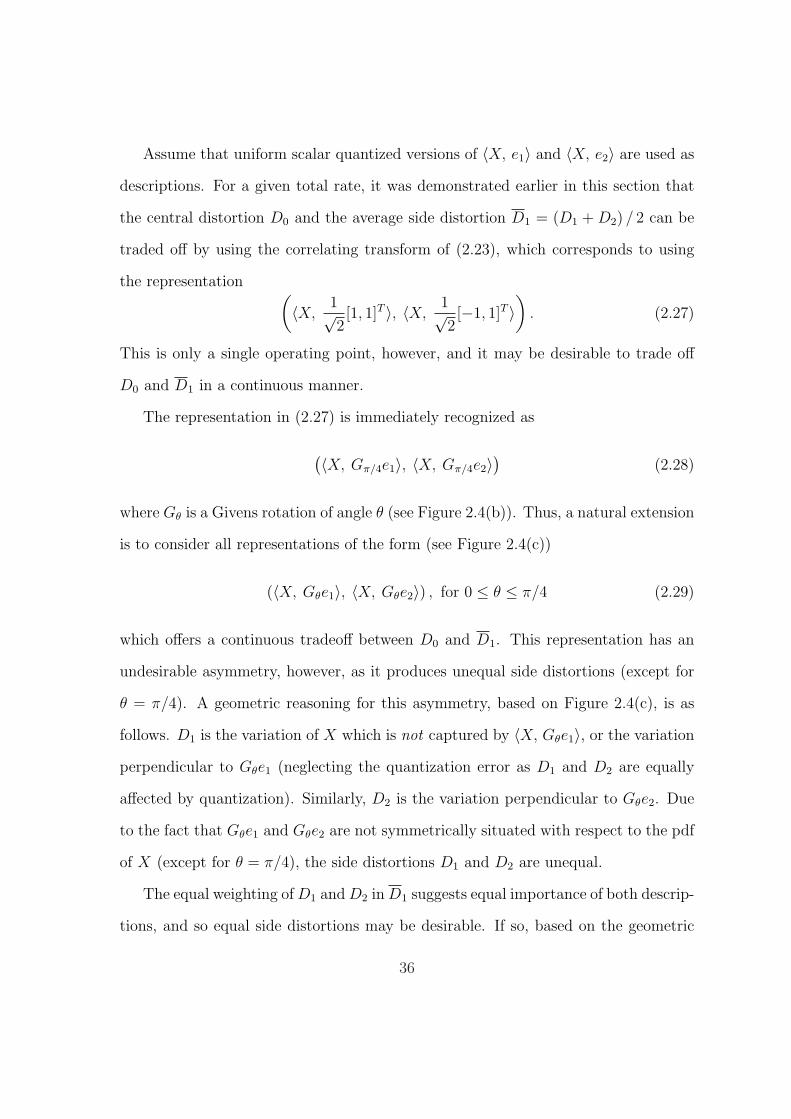
Assume that uniform scalar quantized versions of 〈X, e1〉 and 〈X, e2〉 are used as

descriptions. For a given total rate, it was demonstrated earlier in this section that

the central distortion D0 and the average side distortion D1 = (D1 + D2) / 2 can be

traded off by using the correlating transform of (2.23), which corresponds to using

the representation (〈X,

1√2[1, 1]T 〉, 〈X,

1√2[−1, 1]T 〉

). (2.27)

This is only a single operating point, however, and it may be desirable to trade off

D0 and D1 in a continuous manner.

The representation in (2.27) is immediately recognized as

(〈X, Gπ/4e1〉, 〈X, Gπ/4e2〉)

(2.28)

where Gθ is a Givens rotation of angle θ (see Figure 2.4(b)). Thus, a natural extension

is to consider all representations of the form (see Figure 2.4(c))

(〈X, Gθe1〉, 〈X, Gθe2〉) , for 0 ≤ θ ≤ π/4 (2.29)

which offers a continuous tradeoff between D0 and D1. This representation has an

undesirable asymmetry, however, as it produces unequal side distortions (except for

θ = π/4). A geometric reasoning for this asymmetry, based on Figure 2.4(c), is as

follows. D1 is the variation of X which is not captured by 〈X, Gθe1〉, or the variation

perpendicular to Gθe1 (neglecting the quantization error as D1 and D2 are equally

affected by quantization). Similarly, D2 is the variation perpendicular to Gθe2. Due

to the fact that Gθe1 and Gθe2 are not symmetrically situated with respect to the pdf

of X (except for θ = π/4), the side distortions D1 and D2 are unequal.

The equal weighting of D1 and D2 in D1 suggests equal importance of both descrip-

tions, and so equal side distortions may be desirable. If so, based on the geometric

36

observation above, it is reasonable to represent X by (see Figure 2.4(d))

(〈X, Gθe1〉, 〈X, G−θe1〉) , for 0 < θ < π/2. (2.30)

Additionally, note that in order to capture most of the principal component of the

source, the basis should be skewed toward e1 (see Figure 2.4(d)). Although equal side

distortions are attained using this representation (i.e., D1 = D2), its use introduces

a new problem.

The representation of X using (2.30) is a nonorthogonal basis expansion (for

θ �= π/4). The uniform scalar quantization of such a representation produces non-

square partition cells. These non-square partition cells are undesirable as they have

normalized second moments that are higher than those of square cells, and thus may

lead to higher distortions [22]. The insight attributed to Vaishampayan is that a

correlating transform can be applied after quantization has been performed in an

orthogonal basis representation, which ensures that the partition cells are square

regardless of the transform. The advantage of this approach over the original method

of pairwise correlating transforms was demonstrated in [39]. Although the transform

in this case maps from a discrete set to a discrete set, it can be designed to approximate

a linear transform [23, 24].

From the geometric view of Figure 2.4, one can easily understand the significance

of the ratio σ1/σ2 in MD coding using correlating transforms. When σ1/σ2 → 1, the

level curves become circles and the variation perpendicular to either basis vector is

then invariant to the basis; the side distortions are thus unaffected by the correlating

transform and this holds equally well for both orthogonal and nonorthogonal bases.

The MD coding technique of correlating transforms can also be generalized to

the case of more than two descriptions. Such an extension is described and analyzed

37

in [24].

38

Chapter 3

Multiple Description Image

Coding via Polyphase Transform

This chapter reviews an efficient technique for MD image coding utilizing a polyphase

transform and selective quantization [30]. This method forms the framework of our

proposed context-based MD coding system, introduced in Chapter 4.

3.1 System Outline

Unlike many other MD coding techniques, such as MD scalar quantization and MD

correlating transforms (both are described in Chapter 2), the technique of MD coding

via polyphase transform and selective quantization explicitly separates description

generation and redundancy addition. This separation can significantly reduce the

complexity of the system design and implementation, especially in the case of more

than two descriptions. The polyphase transform-based technique described in this

chapter also enables to easily generate descriptions of statistically equal rate and

39

importance, a property which is well suited to communication systems with no priority

mechanisms for data delivery, such as the Internet.

For description generation, this approach employs a polyphase transform (i.e.,

decomposition to polyphase-like components; specific options are described below),

and each of the resulting polyphase components is coded independently at a source

coding rate to constitute the primary part of information for its corresponding de-

scription. In order to explicitly add redundancy to each description, other polyphase

components are then coded at a (usually lower) redundancy coding rate using se-

lective quantization and added to this description. In case of channel failures, this

redundancy enables an acceptable reconstruction of the lost components. This is

shown in Figure 3.1 for the two-description case.

Z-1

Q1

Q1

MUX

MUX

DMUX

DMUX

Q2

Q2

2

2

Q1-1

Q1-1

Q2-1

Q2

-1

2

2

2

2 Z

Z

+

+

+

X(1)^

X(0)^

X(2)^

X

Y1

Y2

Channel 1

Channel 2

Figure 3.1: MD coding system based on polyphase transform and selectivequantization.

Referring to Figure 3.1, the input X is first decomposed into two sub-sources Y1

and Y2 via a polyphase transform. Each of the two polyphase components Y1 and Y2

40

is then quantized independently by Q1 to form the primary part of information for its

corresponding description. In order to enable an acceptable reconstruction of the lost

component in the case of a channel failure, each description also carries information

about the other component—a coarsely1 quantized version produced by the quantizer

Q2. The outputs of the appropriate quantizers are combined together by a multiplexer

to form the descriptions, and each description is transmitted on its corresponding

channel. At the receiver, if both descriptions arrive, the finely quantized versions of

the two polyphase components (produced by Q1 during encoding) are then used for

reconstruction to produce X(0). If one of the descriptions is lost, one finely quantized

and one coarsely quantized polyphase component (the primary and redundant part of

the received description, respectively) are used for reconstruction (the reconstruction

from description i only is denoted by X(i), i = 1, 2).

Note that in the encoded bit stream the redundant information (coarsely quan-

tized polyphase components) is explicitly separated from the primary information

(finely quantized polyphase components), which simplifies the design and implemen-

tation of the encoder and decoders in the system. Compared to the technique of MD

correlating transforms, no use of an additional correlating transform is needed here,

while careful index assignments required by MD scalar quantizers are also avoided

by this approach. Despite the similarity to Jayant’s subsample-interpolation (SI) ap-

proach [28, 29] (described in Section 2.3), the polyphase transform-based technique

does not rely on the existence and amount of redundancy already present in the source

and thus can also be applied to memoryless sources.

1The quantizers Q1 and Q2 are referred to as “fine” and “coarse”, respectively, in order todemonstrate the concept of selective quantization. The actual relation between the resolutions ofthe different quantizers is generally determined according to the probability of description loss (i.e.,channel failure).

41

The polyphase transform-based technique can also be adapted to the case of cor-

related input data, as shown in Figure 3.2. The correlated input data (e.g., an image)

Decorrelating

Transform

Description

Generation

Redundancy

Addition

Quantization &

Entropy Encoding

Packetization &

Synchronization

Input

Channel

Inverse

DecorrelatingTransform

Description

Merging

Recover from

Redundancy

Entropy Decoding &

DequantizationUnpacketization

Output

Figure 3.2: MD coding system based on polyphase transform and selectivequantization for correlated input.

is first transformed by a decorrelating transform (e.g., KLT [22]). In the description

generation stage, a polyphase transform is applied to the transform coefficients and

each resulting polyphase component forms the primary part of a single description.

The redundancy addition stage identifies for each description which of the other de-

scriptions it will protect and introduces redundancy among descriptions accordingly.

Each description is then quantized and entropy-coded independently, where the pri-

mary information is coded at a source coding rate and the redundant information

is coded at a (usually lower) redundancy coding rate. The coded descriptions are

independently packetized and transmitted over the network (e.g., the Internet).

For decoding, the decoder first identifies which descriptions are available and which

are lost. It then decodes the available descriptions and uses the redundancy infor-

mation to reconstruct the polyphase components whose corresponding descriptions

are missing. In the description merging stage the reconstructed polyphase compo-

nents are recomposed together and finally the inverse of the decorrelating transform

is applied to obtain the reconstructed output.

42

3.2 Experimental Results

In this section we review some of the experimental results for the polyphase transform-

based MD image coder, as reported in [30]. It is aimed to demonstrate the perfor-

mance of the polyphase transform-based coder and compare it with that of an al-

ternative MD wavelet image coder based on multiple description scalar quantization

(MDSQ).

For the two-description case, in the polyphase transform-based MD image coder

of [30], the input image is first wavelet transformed and a polyphase transform is

then applied to the wavelet coefficients to decompose them into two polyphase com-

ponents. Two different types of polyphase transform are examined. One is the plain

polyphase transform, which, for each row in each subband, simply groups all the

even-numbered coefficients into one polyphase component and all the odd-numbered

coefficients into the other component. The second, which can be viewed as a gen-

eralized polyphase transform in vector form, groups wavelet coefficients in different

subbands corresponding to the same spatial location into a block structure similar

to the zerotree structure [49]. One polyphase component then consists of all the

even-numbered blocks and the other consists of all the odd-numbered blocks.

Finely quantized and coarsely quantized versions of the polyphase components

then constitute the two descriptions, as explained in Section 3.1. The actual quanti-

zation and entropy coding of the different polyphase components is performed using

the SPIHT wavelet image coder [45].

For the grayscale image Lena of size 512×512 pixels, Figure 3.3 shows2 the PSNR

(Peak Signal-to-Noise Ratio) values corresponding to the central and (average) side

2Figure 3.3 is based on Figure 5(a) from [30], after a swap between the curves referring to theplain and vector-form polyphase transforms, as implied by the accompanying text in [30].

43

distortions obtained for different amounts of redundancy and a total rate of 1 bpp

(bits per pixel). Comparing the results for the two types of polyphase transforms, the

22 24 26 28 30 32 34 36 3836.5

37

37.5

38

38.5

39

39.5

40

40.5

Side PSNR [dB]

Cen

tral P

SN

R [d

B]

Polyphase (plain)Polyphase (vector−form)MDSQ−based

Figure 3.3: Central PSNR vs. side PSNR for image Lena; total rate of 1 bpp. Thepolyphase transform-based MD wavelet coder [30] (with two options for the

polyphase transform) is compared with the MDSQ-based coder [46].

vector-form polyphase transform yields slightly better results than the plain polyphase

transform. This can be explained by the fact that the SPIHT coder is suited to the

zerotree structure used by the vector-form polyphase transform and thus more efficient

coding is obtained for this type of transform. A comparison with the MDSQ-based

44

MD wavelet image coder of Servetto et al. [46] (results are obtained from [30]) is also

shown in Figure 3.3 and demonstrates the effectiveness of the polyphase transform-

based MD coding technique.

45

Chapter 4

Context-Based Multiple

Description Wavelet Image Coding:

Motivation and Proposed System

Outline

This chapter provides the motivation for context-based MD coding in the wavelet

domain, which enables the proposed coder to utilize some useful properties of the

wavelet decomposition for meeting MD coding objectives, and also presents the out-

line of the proposed context-based MD wavelet image coder. The subsequent chapters

will provide a more detailed description of the main building blocks of the proposed

coder. These include the context-based classification procedure, which enables us

to use a set of customized quantizers for improved coding efficiency, as well as the

efficient parametric model-based quantization and bit allocation schemes.

46

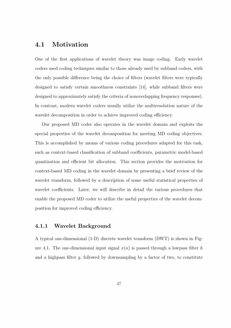
4.1 Motivation

One of the first applications of wavelet theory was image coding. Early wavelet

coders used coding techniques similar to those already used by subband coders, with

the only possible difference being the choice of filters (wavelet filters were typically

designed to satisfy certain smoothness constraints [14], while subband filters were

designed to approximately satisfy the criteria of nonoverlapping frequency responses).

In contrast, modern wavelet coders usually utilize the multiresolution nature of the

wavelet decomposition in order to achieve improved coding efficiency.

Our proposed MD coder also operates in the wavelet domain and exploits the

special properties of the wavelet decomposition for meeting MD coding objectives.

This is accomplished by means of various coding procedures adapted for this task,

such as context-based classification of subband coefficients, parametric model-based

quantization and efficient bit allocation. This section provides the motivation for

context-based MD coding in the wavelet domain by presenting a brief review of the

wavelet transform, followed by a description of some useful statistical properties of

wavelet coefficients. Later, we will describe in detail the various procedures that

enable the proposed MD coder to utilize the useful properties of the wavelet decom-

position for improved coding efficiency.

4.1.1 Wavelet Background

A typical one-dimensional (1-D) discrete wavelet transform (DWT) is shown in Fig-

ure 4.1. The one-dimensional input signal x(n) is passed through a lowpass filter h

and a highpass filter g, followed by downsampling by a factor of two, to constitute

47

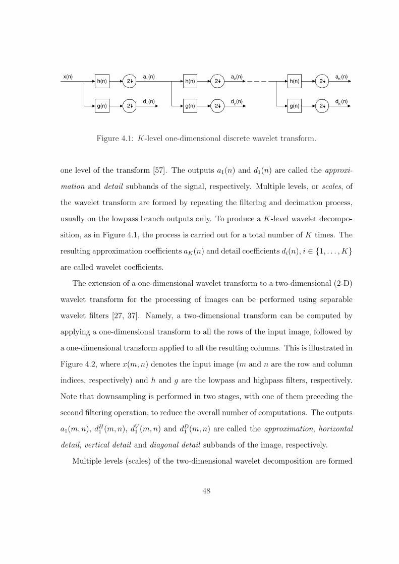
2x(n)

h(n)

2g(n)

a1(n)

d1(n)

2h(n)

2g(n)

a2(n)

d2(n)

2h(n)

2g(n)

aK(n)

dK(n)

Figure 4.1: K-level one-dimensional discrete wavelet transform.

one level of the transform [57]. The outputs a1(n) and d1(n) are called the approxi-

mation and detail subbands of the signal, respectively. Multiple levels, or scales, of

the wavelet transform are formed by repeating the filtering and decimation process,

usually on the lowpass branch outputs only. To produce a K-level wavelet decompo-

sition, as in Figure 4.1, the process is carried out for a total number of K times. The

resulting approximation coefficients aK(n) and detail coefficients di(n), i ∈ {1, . . . , K}are called wavelet coefficients.

The extension of a one-dimensional wavelet transform to a two-dimensional (2-D)

wavelet transform for the processing of images can be performed using separable

wavelet filters [27, 37]. Namely, a two-dimensional transform can be computed by

applying a one-dimensional transform to all the rows of the input image, followed by

a one-dimensional transform applied to all the resulting columns. This is illustrated in

Figure 4.2, where x(m,n) denotes the input image (m and n are the row and column

indices, respectively) and h and g are the lowpass and highpass filters, respectively.

Note that downsampling is performed in two stages, with one of them preceding the

second filtering operation, to reduce the overall number of computations. The outputs

a1(m,n), dH1 (m,n), dV

1 (m,n) and dD1 (m,n) are called the approximation, horizontal

detail, vertical detail and diagonal detail subbands of the image, respectively.

Multiple levels (scales) of the two-dimensional wavelet decomposition are formed

48

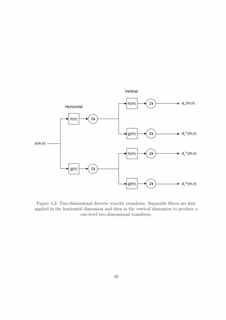
2

x(m,n)

h(n)

2g(n)

2h(m)

2g(m)

a1(m,n)

d1

H(m,n)

2h(m)

2g(m) d1

D(m,n)

d1V(m,n)

Horizontal

Vertical

Figure 4.2: Two-dimensional discrete wavelet transform. Separable filters are firstapplied in the horizontal dimension and then in the vertical dimension to produce a

one-level two-dimensional transform.

49

by repeating the process, typically on the approximation subband only. As an ex-

ample, consider the original image of size 512 × 512 pixels shown in Figure 4.3.

A three-level two-dimensional wavelet transform of the original image is shown in

Figure 4.4. Note that the detail subbands (all subbands except the approximation

subband a3 in the upper left corner of the decomposition) have been enhanced to

make their underlying structure more visible.

The octave-band frequency decomposition, obtained by recursively splitting the

lowpass branch outputs, provides good spatial selectivity at higher frequencies, and

good frequency selectivity at lower frequencies. This tradeoff is very useful for the

analysis of natural images, as these often exhibit short, high-frequency events (e.g.,

edges), in addition to long, low-frequency events (e.g., typical scene’s background).

4.1.2 Statistical Characterization of Wavelet Coefficients

For the purpose of image coding, one of the most attractive properties of the wavelet

transform is its tendency to compact the energy of the input image into a relatively

small number of wavelet coefficients [57]. This energy compaction property can also be

shown to be equivalent to reducing the correlation amongst wavelet coefficients [58].

For natural images, as an example, much of the energy in the wavelet transform is

concentrated in the approximation subband. Moreover, the energy in detail subbands

is concentrated in a relatively small number of coefficients.

The first order statistics (distribution marginals) of detail1 wavelet coefficients

1Approximation coefficients are usually modeled using a uniform distribution [9].

50

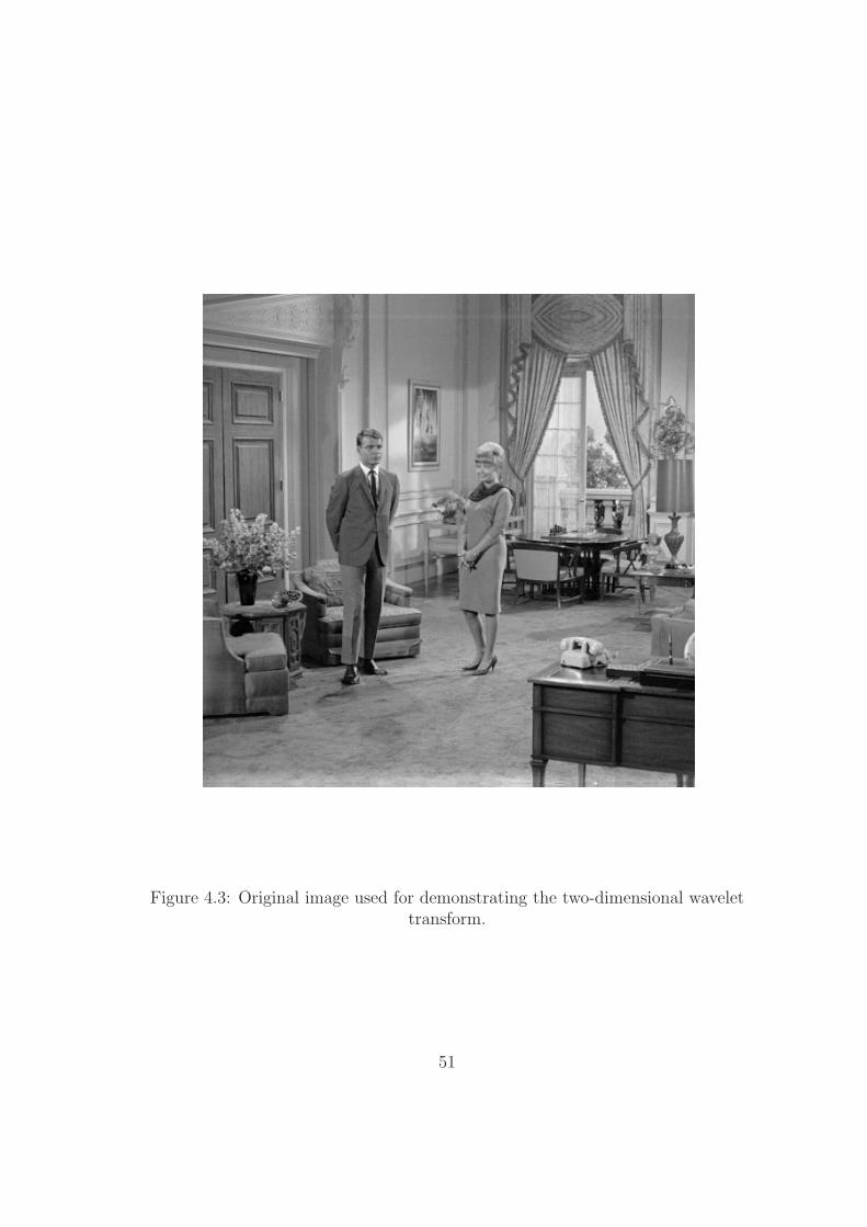
Figure 4.3: Original image used for demonstrating the two-dimensional wavelettransform.

51

Figure 4.4: Example of a three-level two-dimensional wavelet transform of theoriginal image shown in Figure 4.3 (the detail subbands have been enhanced to

make their underlying structure more visible).

52

have been previously modeled [31, 33, 36, 37] using a two-parameter generalized Gaus-

sian (also called generalized Laplacian) probability density function (pdf) of the form

fs,r(x) =1

N(s, r)e−|x/s|r (4.1)

where N(s, r) = 2sΓ(1/r)/r and Γ(a) =∫∞

0ta−1e−t dt is the Gamma function. The

shape parameter r determines the exponential rate of decay and the distribution

variance σ2 is given by

σ2 =s2Γ

(3r

)Γ(

1r

) . (4.2)

The generalized Gaussian distribution (GGD) is a family of zero-mean symmetric

distributions that include the Laplacian distribution (for r = 1) and the Gaussian

distribution (for r = 2). In addition, the density function of (4.1) converges pointwise

to a uniform density on (−s, s) as r → ∞.

For various types of images, excellent fits of the generalized Gaussian probability

density function of (4.1) have been demonstrated in [9]. For the images in the rich

sample set used in [9], the shape parameter r in (4.1) corresponding to the best fit

is typically in the range [0.5, 1], which implies that the first order statistics of detail

wavelet coefficients can be reasonably modeled using a Laplacian distribution.

An example of the generalized Gaussian probability density function of (4.1) with

r = 1 (i.e., Laplacian density) and s = 1.5 is shown in Figure 4.5. As shown, the

density function is symmetric, peaked at zero and has relatively long tails. The long

tails indicate the existence of a few subband coefficients with large magnitudes that

concentrate a large portion of the energy in the subband. The high peak around zero

indicates that most coefficients in the subband have magnitudes which are close to

zero and thus have low energy.

Although the coefficients produced by the wavelet transform are approximately

53

−10 −5 0 5 100

0.05

0.1

0.15

0.2

0.25

0.3

0.35

x

f(x)

Figure 4.5: The generalized Gaussian probability density function of (4.1) withr = 1 and s = 1.5.

54

decorrelated [49], visual inspection of the wavelet decomposition (see Figure 4.4, for

example) reveals that wavelet coefficients are not statistically independent. In fact,

large magnitude coefficients are usually gathered at neighboring spatial locations, as

well as at the same relative spatial locations of subbands at adjacent scales and orien-

tations [9]. Experiments show that the correlation coefficient between the square of a

wavelet coefficient and the square of the coefficient corresponding to the same spatial

location at the next coarser scale (also called parent ; see Figure 4.6 for illustration)

tends to be between 0.2 and 0.6 with a concentration around 0.35 [49].

Numerous image compression schemes implicitly utilize the spatial and scale-to-

scale dependencies present in the wavelet decomposition. The embedded zerotree

wavelet (EZW) coder of Shapiro [49], whose introduction in 1993 marked the begin-

ning of the era of modern lossy wavelet coding, exploits the likelihood of a coefficient

to have small magnitude if the coefficients corresponding to the same spatial location

at coarser scales have small magnitudes. In this technique, entire trees of zeros are

encoded with a single symbol, thus capturing a portion of the conditional distribu-

tion of a coefficient given the coefficients corresponding to the same spatial location at

coarser scales. Said and Pearlman [45] generalized Shapiro’s zerotrees and introduced

set partitioning techniques to effectively encode these generalized trees of zeros. The

resulting coding scheme, known as SPIHT (Set Partitioning In Hierarchical Trees),

outperforms EZW at even lower levels of complexity. LoPresto et al. [36] use a gener-

alized Gaussian model for the wavelet coefficients and estimate the model parameters

from local neighborhoods.

In order to explicitly examine and utilize the statistical relationship between the

magnitudes of wavelet coefficients, and due to the difficulty of characterizing the full

55

CousinCLeft

Up

Cousin

AuntParent

Aunt

di+1

Ddi+1

V

di+1

H

diV d

iD

diH

Figure 4.6: Potential conditioning neighbors (also at adjacent scales andorientations) for a given wavelet coefficient C.

56

multidimensional density, Buccigrossi and Simoncelli [9] proposed to use a linear pre-

dictor for the magnitude of a coefficient, based on the magnitudes of its neighbors

(also at adjacent scales and orientations), as shown in Figure 4.6. In order to deter-

mine which coefficients to include in the conditioning set, rather than exhaustively

explore all possible subsets of candidate neighbors, a greedy algorithm was applied.

Specifically, the conditioning set was constructed incrementally: at each step, the

remaining neighbor whose inclusion maximized the mutual information between the

coefficent and its predictor was joined to the conditioning set. Using this analysis

based on three sample images, and imposing causality (assuming a standard scanline

ordering of the coefficients), it was found that the local neighbors within the subband

(labeled “Left” and “Up” in Figure 4.6) contributed the most to the mutual informa-

tion. The parent and the cousins (in that order) followed with smaller contributions,

while joining any of the remaining potential neighbors to the conditioning set offered

only a marginal increase in the resulting mutual information.

As described above, the utilization of the statistical dependencies present in the

wavelet decomposition enables modern wavelet coders to achieve improved coding

efficiency. The proposed context-based MD wavelet image coder, introduced in the

following section, is designed to utilize the fundamental properties of the wavelet

decomposition in the framework of multiple description coding. In the following

sections, we will show how these useful properties of the wavelet decomposition can

be exploited for meeting MD coding objectives.

57

4.2 Proposed System Outline

Chapter 3 described a useful technique for MD coding via the utilization of a polyphase

transform and selective quantization [30]. Section 4.1 introduced the wavelet decom-

position and its fundamental statistical properties. Our proposed context-based MD

wavelet image coding system is aimed to provide improved coding efficiency by means

of effective utilization of the statistical properties of the wavelet decomposition, in

the general framework of polyphase transform-based MD coding. We focus on the

two-description case, mainly due to its tractability, as is common in the MD coding

literature.

For image coding (i.e., correlated input data), the polyphase transform-based tech-

nique of [30] first employs a decorrelating transform, such as wavelet transform. Re-

ferring to Figure 3.1 in Section 3.1 (which does not show the decorrelating transform

itself), the resulting decorrelated transform coefficients, denoted by X, are decom-

posed into two sub-sources Y1 and Y2 via a polyphase transform. Each of the two

polyphase components Y1 and Y2 is then quantized independently by Q1 to form the

primary part of information for its corresponding description. In order to enable an

acceptable reconstruction of the lost component in the case of a channel failure, each

description also carries information about the other component—a coarsely quan-

tized version produced by the quantizer Q2. At the receiver, if both descriptions

arrive, the finely quantized versions of the two polyphase components (produced by

Q1 during encoding) are used for reconstruction. If one of the descriptions is lost, one

finely quantized and one coarsely quantized polyphase component (the primary and

redundant part of the received description, respectively) are used for reconstruction.

As also pointed out in [30], the structural similarities existing between the polyphase

58

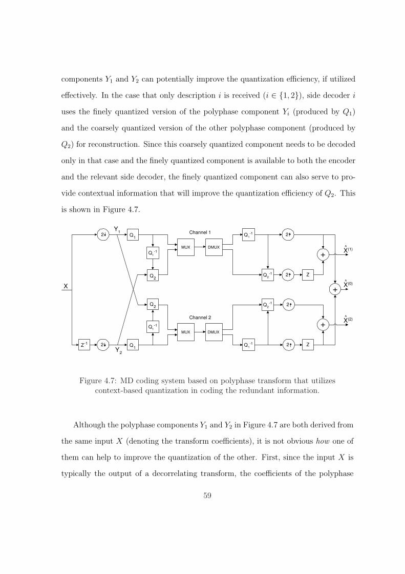
components Y1 and Y2 can potentially improve the quantization efficiency, if utilized

effectively. In the case that only description i is received (i ∈ {1, 2}), side decoder i

uses the finely quantized version of the polyphase component Yi (produced by Q1)

and the coarsely quantized version of the other polyphase component (produced by

Q2) for reconstruction. Since this coarsely quantized component needs to be decoded

only in that case and the finely quantized component is available to both the encoder

and the relevant side decoder, the finely quantized component can also serve to pro-

vide contextual information that will improve the quantization efficiency of Q2. This

is shown in Figure 4.7.

Z-1

Q1

Q1

MUX

MUX

DMUX

DMUX

Q2

Q2

2

2

Q1-1

Q1-1

Q2-1

Q2

-1

2

2

2

2 Z

Z

+

+

+

X(1)^

X(0)^

X(2)^

X

Y1

Y2

Q1-1

Q1-1

Channel 1

Channel 2

Figure 4.7: MD coding system based on polyphase transform that utilizescontext-based quantization in coding the redundant information.

Although the polyphase components Y1 and Y2 in Figure 4.7 are both derived from

the same input X (denoting the transform coefficients), it is not obvious how one of

them can help to improve the quantization of the other. First, since the input X is

typically the output of a decorrelating transform, the coefficients of the polyphase

59

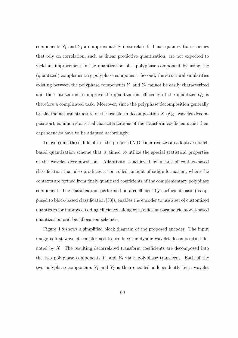
components Y1 and Y2 are approximately decorrelated. Thus, quantization schemes

that rely on correlation, such as linear predictive quantization, are not expected to

yield an improvement in the quantization of a polyphase component by using the

(quantized) complementary polyphase component. Second, the structural similarities

existing between the polyphase components Y1 and Y2 cannot be easily characterized

and their utilization to improve the quantization efficiency of the quantizer Q2 is

therefore a complicated task. Moreover, since the polyphase decomposition generally

breaks the natural structure of the transform decomposition X (e.g., wavelet decom-

position), common statistical characterizations of the transform coefficients and their

dependencies have to be adapted accordingly.

To overcome these difficulties, the proposed MD coder realizes an adaptive model-

based quantization scheme that is aimed to utilize the special statistical properties

of the wavelet decomposition. Adaptivity is achieved by means of context-based

classification that also produces a controlled amount of side information, where the

contexts are formed from finely quantized coefficients of the complementary polyphase

component. The classification, performed on a coefficient-by-coefficient basis (as op-

posed to block-based classification [33]), enables the encoder to use a set of customized

quantizers for improved coding efficiency, along with efficient parametric model-based

quantization and bit allocation schemes.

Figure 4.8 shows a simplified block diagram of the proposed encoder. The input

image is first wavelet transformed to produce the dyadic wavelet decomposition de-

noted by X. The resulting decorrelated transform coefficients are decomposed into

the two polyphase components Y1 and Y2 via a polyphase transform. Each of the

two polyphase components Y1 and Y2 is then encoded independently by a wavelet

60

Y1

Y2

Channel 1

Channel 2

Polyphase

Transform

Original

Image

Wavelet

Coefficients

Encoder

Context-Based

Classification

Model-Based

Quantization

Entropy

Encoding

Side

Information

Wavelet

Coefficients

Encoder

Context-Based

Classification

Model-Based

Quantization

Entropy

Encoding

Wavelet

Transform

X

Side

Information

Primary

Information

Redundant

Information

Redundant

Information

Primary

Information

Quantized

Coefficients

Quantized

Coefficients

Figure 4.8: Simplified block diagram of the proposed MD encoder.

coefficients encoder to form the primary part of information for its corresponding de-

scription. Depending on the exact type of polyphase transform, this can generally be a

standard wavelet encoder (e.g., SPIHT [45] encoder), operating directly on the wavelet

coefficients. In order to enable an acceptable reconstruction of the lost component in

the case of a channel failure, each description also carries information about the other

component. This redundant information, useful only in the case of a lost description,

is produced by efficient algorithms for classification, bit allocation, quantization, and

adaptive entropy encoding, that use contextual information extracted from quantized

coefficients of the complementary polyphase component. These quantized coefficients

are obtained directly from the wavelet coefficients encoder that produces the primary

part of information for the description.

61

In order to utilize the statistical dependencies between neighboring wavelet co-

efficients (see Section 4.1.2), for improving the coding efficiency of the redundant

information, the context used for the classification of a given coefficient is formed

from neighboring quantized coefficients, obtained from the complementary polyphase

component. To avoid the need for an explicit characterization of the statistical depen-

dencies between neighboring coefficients, we use an adaptive classification procedure

that also produces a controlled amount of side information, which is transmitted to

the decoder. This side information includes the classification thresholds, allowing to

select a class for a coefficient given its context, as well as the source statistics of each

class, where each class is modeled using a parametric distribution. The paramet-

ric modeling is also utilized by the bit allocation, quantization and entropy coding

procedures that follow.

A simplified block diagram of the corresponding decoder is shown in Figure 4.9.

If both descriptions arrive, the primary part of information from each description is

decoded using a wavelet coefficients decoder (corresponding to the wavelet coefficients

encoder used for encoding the primary part of information). The central decoder then

composes the resulting polyphase components to produce the reconstructed wavelet

decomposition X(0). Finally, an inverse wavelet transform is applied to the recovered

wavelet coefficients to produce the reconstructed image.

If only description i is received (i ∈ {1, 2}), the primary part of information from

the received description is decoded, as before, to recover the quantized polyphase

component Yi. The complementary polyphase component is then recovered from the

redundant part of information. To this end, entropy decoding is performed, followed

by context-based classification and dequantization. The contexts for classification are

formed from quantized coefficients of the polyphase component Yi, and the auxiliary

62

Channel 1

Channel 2

Inverse

Polyphase

Transform

Image

Reconstructed By

Side Decoder 1

Wavelet

Coefficients

Decoder

Entropy

Decoding

Context-Based

ClassificationDequantization

Inverse

Wavelet

Transform

X(1)^

Inverse

Polyphase

Transform

Inverse

Wavelet

Transform

X(0)^

Side

Information

Side

Information

Primary

Information

Redundant

Information

Redundant

Information

Primary

Information

Wavelet

Coefficients

Decoder

Entropy

Decoding

Context-Based

ClassificationDequantization

Inverse

Polyphase

Transform

Image

Reconstructed By

Side Decoder 2

Inverse

Wavelet

Transform

Image

Reconstructed By

Central Decoder

X(2)^

Quantized

Coefficients

Quantized

Coefficients

Figure 4.9: Simplified block diagram of the proposed MD decoder.

side information provides the required classification thresholds and source statistics

of each class. Side decoder i then composes the recovered polyphase components to

produce the reconstructed wavelet decomposition X(i). An inverse wavelet transform

follows to produce the reconstructed image.

The next chapters provide a detailed description of the main building blocks of

the proposed coder, which include the classification, quantization and bit allocation

schemes. A careful treatment of some important implementation considerations, such

as boundary extension and optimal bit allocation for biorthogonal wavelet filters, is

also provided.

63

Chapter 5



Context-Based Classification

5.1 Introduction

Data classification is an effective technique used in various quantization applications.

For an input source modeled as a mixture of sources with different distributions,

classification enables the use of a set of quantizers, each customized to an individual

distribution component. Compared to the use of a single average quantizer fitted to

the overall input statistics, this offers a potential increase in coding efficiency, since the

quantization can be adapted to the data based on the classification information [66].

As a simple demonstration of the potential benefit of classification in general

subband image coding applications, consider Figure 4.4 (in Section 4.1.2), which

shows the wavelet transform of the natural image shown in Figure 4.3. As can be

64

seen, high-activity regions (corresponding to edges in the image, for example) tend

to cluster at neighboring spatial locations, and are separated from surrounding low-

activity regions. Identifying those high- and low-activity regions via classification

would enable the utilization of separate quantizers, each suited to a different region.

A comprehensive study by Joshi et al. [33] demonstrates substantial coding gains

due to classification in subband image coding applications. The considered classifica-

tion techniques are all based on block-wise classification, where one of a finite number

of classes is assigned to each block of coefficients within a subband. In the framework

of [33], the class assigned to each block is explicitly stated as side information and

transmitted to the decoder (this is known as forward classification). In order to limit

the resulting overhead, the size of blocks used for classification must be large enough,

and the number of potential classes must be kept small. Even then, however, the

overhead rate may become excessive for low target bit rates.

Our proposed MD coder utilizes classification for efficient coding of the redundant

information, which enables an acceptable reconstruction of the lost polyphase com-

ponent in the case of a channel failure. In order to perform well across a wide range

of total bit rates (corresponding to the desired quality of reconstruction) and redun-

dancy levels (derived from the probability of channel failure), the proposed coder

avoids the penalty of forward classification. To this end, the classification is based on

quantized coefficients of the complementary polyphase component, and utilizes the

special statistical properties of the wavelet decomposition. Since the quantized coef-

ficients of the complementary polyphase component are also available at the decoder,

no transmission of side information is required. Nevertheless, a controlled amount

of side information is still produced and transmitted to the decoder, in order to im-

prove the performance of the system. This side information includes the classification

65

thresholds, allowing to select a class for a coefficient given its context, as well as the

source statistics of each class, where each class is modeled using a parametric distri-

bution. It allows the classification process to adapt itself to the data, and enables

the proposed coder to avoid the need for an explicit characterization of the statisti-

cal dependencies between neighboring wavelet coefficients. Compared to block-based

classification techniques, our context-based classification procedure, inspired by that

of [66], enables finer grain classification, down to the coefficient level (rather than a

block level).

For description i ∈ {1, 2}, define the polyphase component Yi to be the primary

polyphase component, and define the complementary component to be the redundant

polyphase component. The context of a given wavelet coefficient in the redundant

polyphase component, is then defined as a set of quantized coefficients from the pri-

mary polyphase component, which is used to characterize the given coefficient. Note

that since the coefficients that form the context are already quantized, the decoder

can use the exact same context used by the encoder. As described in Section 4.1.2,

significant statistical dependencies exist between neighboring wavelet coefficients, and

these can be utilized for efficient context-based classification. For a given coefficient

in the redundant polyphase component, we therefore form a context from neighboring

quantized coefficients that belong to the primary polyphase component. Assuming a

plain polyphase transform, which, for each column in each subband, simply groups

all the odd-numbered coefficients into one polyphase component and all the even-

numbered coefficients into the other component, Figure 5.1 shows the context of a

given wavelet coefficient Xi,j. For the ease of illustration, the primary and redundant

polyphase components are interleaved in the figure. As shown, the classification of

66

Xi+1,j-1

Xi-1,j-1

Xi,j

Xi-1,j

Xi-1,j+1

Xi+1,j

Xi+1,j+1

Primary polyphase component

Redundant polyphase component

Figure 5.1: Context of a given wavelet coefficient Xi,j. The coefficient belongs to theredundant polyphase component, and is shown in black. The quantized coefficientsthat form the context belong to the primary polyphase component, and are shown

in white.

67

the wavelet coefficient Xi,j is based on the following context:

Ci,j ={

Xi−1,j−1, Xi−1,j, Xi−1,j+1, Xi+1,j−1, Xi+1,j, Xi+1,j+1

}(5.1)

where X denotes the value of X after quantization by the wavelet coefficients encoder

(see Figure 4.8), and the coordinate system refers to the whole subband (i.e, prior to

the polyphase transform).

5.2 Classification Rule

We now turn to describe the classification rule, which assigns one of a finite number of

classes to a coefficient Xi,j, given its context Ci,j. Due to the difficulty of characterizing

the full multidimensional relationship between the magnitudes of neighboring wavelet

coefficients, the classification rule is based on a weighted average of the magnitudes

of coefficients in Ci,j. Define the activity Ai,j of the coefficient Xi,j, predicted from its

context Ci,j, as

Ai,j = a1|Xi−1,j−1|+ a2|Xi−1,j|+ a3|Xi−1,j+1|+ a4|Xi+1,j−1|+ a5|Xi+1,j|+ a6|Xi+1,j+1|(5.2)

where the fixed relative weights {ak} satisfy∑

k ak = 1. One reasonable choice is to

set the weights {ak} in accordance to the distances of the corresponding neighboring

coefficients from the current coefficient Xi,j, such that closer coefficients will have

greater contribution to the activity Ai,j compared to more distant ones. In the pro-

posed coder we thus set the weights {ak} to be inversely proportional to the Euclidean

distances of the corresponding coefficients in Ci,j from the coefficient Xi,j.

In order to classify a coefficient Xi,j, its context Ci,j is first used to predict its activ-

ity Ai,j. The (nonnegative) activity Ai,j is then compared with a set of pre-computed

68

adaptive classification thresholds to determine the class assigned to Xi,j. Specifi-

cally, assuming N + 1 potential classes C0, C1, . . . , CN , and given N monotonically

increasing classification thresholds

T0 = 0 < T1 < T2 < · · · < TN−1 < ∞ , (5.3)

the coefficient Xi,j is assigned to the class Ck if

Ai,j ∈ (Tk−1, Tk] (5.4)

where T−1 = −∞ and TN = ∞. This is shown in Figure 5.2.

Ai,j

C0

C1

C2

CN-1

CN

T0=0 T

1T

2T

N-2T

N-1T

-1= - 8 T

N= 8

Figure 5.2: Classification of the coefficient Xi,j based on its activity Ai,j.

Note that since the activity is a nonnegative quantity, a coefficient Xi,j is assigned

to the class C0 if and only if Ai,j = 0. In other words, a coefficient is assigned to

C0 if and only if all the coefficients in its context are quantized to zero. This special

case is more common at finer scales of the wavelet decomposition, and becomes more

dominant at lower bit rates (with respect to the primary polyphase component, from

which the context is extracted). In order to reliably model these coefficients having

an all-zero context, a special class, namely C0, is assigned only to them. This class is

also called the zero-context class.

69

5.3 Classification Thresholds Design

This section describes in detail the classification thresholds design—the procedure to

adaptively determine the classification thresholds T1, T2, . . . , TN−1, with the goal of

maximizing the coding gain due to classification. This procedure is performed inde-

pendently for each of the subbands. In order to enable the decoder to perform the

same classification as the encoder, the classification thresholds are also transmitted

to the decoder as side information (in addition to the parametric source statistics of

each class). Note that if we had also included in the context Ci,j already quantized

coefficients of the redundant polyphase component, an interdependency between the

classification and the choice of quantizers for encoding the redundant polyphase com-

ponent would have been created. Namely, in such a case, the choice of quantizers

for encoding the redundant polyphase component would have influenced the classifi-

cation and vice versa. We therefore refrain from including in Ci,j already quantized

coefficients of the redundant polyphase component, and so Ci,j is formed solely from

quantized coefficients of the primary polyphase component. Thus, the process is nat-

urally performed in a serial manner: the classification thresholds are determined first,

then actual classification is performed, and only then the selection of quantizers is

considered.

As will be detailed in Chapter 6, our class-adaptive quantization is based on a

parametric distribution model. Specifically, we assume that the coefficients in each

class of each subband are drawn from a (zero-mean) Laplacian distribution. Since

we employ a predictive (DPCM-like) quantization scheme to encode the coefficients

in the approximation subband (as will be described in Section 7.2.1), we assume a

Laplacian distribution model (for the prediction errors) in the approximation subband

70

as well.

The classification thresholds design involves estimation of the Laplacian distribu-

tion’s parameter for each candidate class. We now derive the maximum likelihood

estimator (MLE) [34, Ch. 7] for this case. Let x1, x2, . . . , xn be n independent, iden-

tically distributed (i.i.d.) observations from a Laplacian source with an unknown

parameter λ (> 0). That is, independent samples drawn according to the probability

density function (pdf)

fλ(x) =λ

2e−λ|x| . (5.5)

The likelihood function of λ is given by

L(λ) =n∏

i=1

fλ(xi) . (5.6)

Taking the natural logarithm to obtain the log-likelihood function yields

L∗(λ) =n∑

i=1

log fλ(xi) =n∑

i=1

log

(λ

2e−λ|xi|

)= n log

(λ

2

)− λ

n∑i=1

|xi| . (5.7)

Maximization of (5.7) with respect to λ then yields the maximum likelihood estima-

tor (MLE) of λ:

λ =n∑n

i=1 |xi| =1

1n

∑ni=1 |xi| . (5.8)

We now describe how to determine the classification thresholds T1, T2, . . . , TN−1

for a given subband. This design procedure is repeated independently for each of the

subbands, and involves only the coefficients in the relevant subband. For brevity, we

refer to the subband coefficients that belong to the redundant polyphase component

as redundant coefficients, and to those that belong to the primary polyphase com-

ponent as primary coefficients. Given the unquantized redundant coefficients (to be

classified eventually using the obtained thresholds) and the quantized primary coeffi-

cients (that form the contexts for classification), we wish to determine the thresholds

71

T1, T2, . . . , TN−1 , assuming a total of N + 1 classes C0, C1, . . . , CN . Note that since

T0 = 0, there are only N − 1 classification thresholds to determine.

As noted in Section 5.2, a redundant coefficient Xi,j is assigned to the class C0—

the zero-context class—if and only if all the coefficients in its context are quantized

to zero (i.e., Ai,j = 0). Thus, as a preliminary step, we first identify all the redundant

coefficients having an activity of zero. These coefficients (and only them) will be

assigned to the class C0, and are therefore not considered in the classification thresh-

olds design. The parameter λ of the Laplacian distribution for the class C0 is also

estimated at this stage using (5.8), and will be transmitted to the decoder. Note that

we are now left with N “ordinary” potential classes (namely, C1, . . . , CN) and need

to determine N − 1 classification thresholds (namely, T1, . . . , TN−1).

The remainder of the design procedure follows that of [66] and is summarized

below. We start by considering an oversized initial set of N0 −1 candidate thresholds

(where N0 > N)

{Tk, 1 ≤ k ≤ N0 − 1 : 0 < T1 < · · · < TN0−1 < ∞} . (5.9)

This thresholds set defines N0 initial classes {C1, . . . , CN0} by the following classifi-

cation rule: the redundant coefficient Xi,j is assigned to the class Ck if

Ai,j ∈ (Tk−1, Tk] (5.10)

for k = 1, . . . , N0, and with T0 = 0 and TN0 = ∞. After the redundant coefficients

are collected into the N0 initial classes according to the classification rule (5.10), the

maximum likelihood estimator (MLE) of the Laplacian parameter for each class is

computed using (5.8). An iterative greedy algorithm is then applied, which removes

one classification threshold (and one class) at each iteration, until the number of

thresholds is reduced to N − 1. At each iteration, the algorithm merges the pair

72

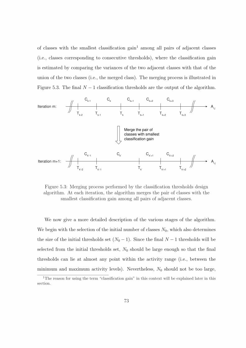
of classes with the smallest classification gain1 among all pairs of adjacent classes

(i.e., classes corresponding to consecutive thresholds), where the classification gain

is estimated by comparing the variances of the two adjacent classes with that of the

union of the two classes (i.e., the merged class). The merging process is illustrated in

Figure 5.3. The final N − 1 classification thresholds are the output of the algorithm.

Ai,j

Ck-1

Ck

Ck+3

Tk-1

Tk

Tk+2

Ck+1

Ck+2

Tk+1

Tk+3

Tk-2

Iteration m:

Ai,j

Ck’-1

Ck’

Ck’+2

Tk’-1

Tk’+1

Ck’+1

Tk’

Tk’+2

Tk’-2

Iteration m+1:

Merge the pair of

classes with smallest

classification gain

Figure 5.3: Merging process performed by the classification thresholds designalgorithm. At each iteration, the algorithm merges the pair of classes with the

smallest classification gain among all pairs of adjacent classes.

We now give a more detailed description of the various stages of the algorithm.

We begin with the selection of the initial number of classes N0, which also determines

the size of the initial thresholds set (N0 − 1). Since the final N − 1 thresholds will be

selected from the initial thresholds set, N0 should be large enough so that the final

thresholds can lie at almost any point within the activity range (i.e., between the

minimum and maximum activity levels). Nevertheless, N0 should not be too large,

1The reason for using the term “classification gain” in this context will be explained later in thissection.

73

in order to enable each of the initial classes to contain enough coefficients, which will

ensure a reliable estimation of the Laplacian parameter for each class. Regarding the

selection of the initial thresholds T1, . . . , TN0−1 themselves, it is desirable that each of

the resulting classes will contain approximately the same number of coefficients, in

order to ensure equally reliable estimates for the different classes. For that reason, the

trivial choice of uniformly spaced thresholds is not appropriate in general. A better

choice is to select N0 − 1 nonuniform thresholds, such that each of the initial classes

will contain approximately the same number of coefficients.

As explained earlier, the greedy algorithm removes one classification threshold

(and one class) at each iteration, until the number of thresholds is reduced to N−1. At

each iteration, the algorithm merges the pair of classes with the smallest classification

gain among all pairs of adjacent classes. Denote the number of coefficients in two

adjacent classes Ck and Ck+1 by nk and nk+1, respectively. Also, let σ2k and σ2

k+1 be

the respective variances of the two classes, and let σ2k′ be the variance of the union of

the two classes. As in [32], the classification gain is then estimated by

G =σ2

k′

σ2rkk σ

2rk+1

k+1

(5.11)

where rk = nk/(nk + nk+1) and rk+1 = 1 − rk = nk+1/(nk + nk+1). We also note

that under certain simplifying assumptions stated in [32], the potential gain in cod-

ing performance due to classification (rather than using one unified class) can be

approximated by a ratio similar to (5.11), which is the reason for referring to G as

the “classification gain” in this context.

Assuming that the Laplacian model is still valid for the union of the classes Ck

and Ck+1, the maximum likelihood estimator (MLE) of the Laplacian parameter for

74

the merged class can be computed as

λk′ =nk + nk+1

nk/λk + nk+1/λk+1

(5.12)

where λk and λk+1 are the parameter estimates for Ck and Ck+1, respectively. This

stems directly from (5.8). Under the Laplacian assumption, the variance is equal to

2/λ2 and thus the classification gain can be estimated by

G = G(λk, λk+1; nk, nk+1) =λ2rk

k λ2rk+1

k+1

λ2k′

. (5.13)

As proved in Appendix A, since the classification gain G of (5.13) is virtually the

ratio of a weighted arithmetic mean to a weighted geometric mean, it follows that

G ≥ 1, with equality if and only if λk = λk+1.

It should be noted that the utilization of the Laplacian model offers a consider-

able reduction in the complexity of the algorithm. Once the Laplacian parameter

estimates for the initial classes are computed, there is no need to use the direct MLE

computation of (5.8) at subsequent iterations. Instead, new parameter estimates

can be obtained using (5.12), without affecting the other classes not involved in the

merging, and the classification gains can be computed directly using (5.13).

The entire classification thresholds design procedure (for a given subband) under

the Laplacian model assumption is summarized as follows.

Algorithm 5.1 (Classification Thresholds Design) Given the unquantized re-

dundant coefficients, the quantized primary coefficients, the desired total number of

classes N + 1, and N0 − 1 initial thresholds (where N0 > N) corresponding to the

initial thresholds set (5.9):

1. Classify all the redundant coefficients with Ai,j = 0 to C0 (the zero-context

class). Compute the corresponding Laplacian parameter estimate λ0 using (5.8).

These coefficients are not considered further by the algorithm.

75

2. Classify the remaining redundant coefficients according to (5.10). Compute the

Laplacian parameter estimates λ1, . . . , λN0 using (5.8). Set K = N0.

3. Find k∗ such that

k∗ = arg min1≤k<K

G(λk, λk+1; nk, nk+1)

where G(·) is given by (5.13) and computed also using (5.12).

4. Merge the classes Ck∗ and Ck∗+1 and update accordingly:

• For k = k∗: Ck = Ck∗⋃

Ck∗+1, nk = nk∗ + nk∗+1, update λk according

to (5.12).

• For k > k∗: Ck = Ck+1, Tk = Tk+1, nk = nk+1, λk = λk+1.

5. Set K = K − 1. If K > N , go to step 3.

6. Finish: return the classification thresholds T1, . . . , TN−1 and the Laplacian pa-

rameter estimates λ0, λ1, . . . , λN .

The procedure is performed separately for each of the descriptions, and is repeated for

each of the subbands. For each description, the corresponding classification thresh-

olds and Laplacian parameter estimates are transmitted to the decoder as side in-

formation. Denoting the number of subbands by S, this involves transmission of

S · [(N − 1) + (N + 1)] = 2NS real numbers (after proper quantization), per de-

scription. The parametric source statistics of the various classes (i.e., the Laplacian

parameter estimates), enable us to further utilize efficient bit allocation and quanti-

zation schemes, as described in the next chapter.

76

Chapter 6



Quantization and Optimal Bit

Allocation

6.1 Parametric Model-Based Uniform Threshold

Quantization

As noted in Section 4.1.2, detail wavelet coefficients can be effectively modeled using

a Laplacian distribution. Naturally, the more general option of using the generalized

Gaussian distribution (GGD) to model the detail coefficients, will always provide a

fit to the empirical distribution which is at least as good as that of the Laplacian

(assuming that the model parameters can be accurately estimated). Nevertheless,

77

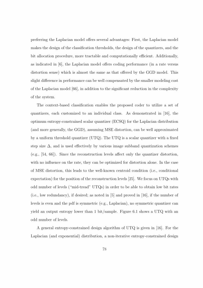
preferring the Laplacian model offers several advantages: First, the Laplacian model

makes the design of the classification thresholds, the design of the quantizers, and the

bit allocation procedure, more tractable and computationally efficient. Additionally,

as indicated in [6], the Laplacian model offers coding performance (in a rate versus

distortion sense) which is almost the same as that offered by the GGD model. This

slight difference in performance can be well compensated by the smaller modeling cost

of the Laplacian model [66], in addition to the significant reduction in the complexity

of the system.

The context-based classification enables the proposed coder to utilize a set of

quantizers, each customized to an individual class. As demonstrated in [16], the

optimum entropy-constrained scalar quantizer (ECSQ) for the Laplacian distribution

(and more generally, the GGD), assuming MSE distortion, can be well approximated

by a uniform threshold quantizer (UTQ). The UTQ is a scalar quantizer with a fixed

step size Δ, and is used effectively by various image subband quantization schemes

(e.g., [54, 66]). Since the reconstruction levels affect only the quantizer distortion,

with no influence on the rate, they can be optimized for distortion alone. In the case

of MSE distortion, this leads to the well-known centroid condition (i.e., conditional

expectation) for the position of the reconstruction levels [25]. We focus on UTQs with

odd number of levels (“mid-tread” UTQs) in order to be able to obtain low bit rates

(i.e., low redundancy), if desired; as noted in [5] and proved in [16], if the number of

levels is even and the pdf is symmetric (e.g., Laplacian), no symmetric quantizer can

yield an output entropy lower than 1 bit/sample. Figure 6.1 shows a UTQ with an

odd number of levels.

A general entropy-constrained design algorithm of UTQ is given in [16]. For the

Laplacian (and exponential) distribution, a non-iterative entropy-constrained design

78

x

b1

b2

f(x)

b3

bL

b-L

b-3

b-2

b-1

q1

q2

qL

q-L

q-2

q-1

q0

Figure 6.1: Uniform threshold quantizer (UTQ) with step size Δ and an oddnumber of levels N = 2L + 1. The bin boundaries are denoted by {bj} and thereconstruction levels by {qj}. The Laplacian pdf is also shown for illustration.

algorithm of UTQ is provided by Sullivan [53]. Due to the relatively high complexity

of the aforementioned design algorithms, we employ a more efficient design strategy:

As detailed in the following section, the proposed coder utilizes an effective optimal

bit allocation scheme, which is based on a pre-designed array of optimized UTQs of

different step sizes (where the optimization is for minimum MSE distortion). This

enables us to greatly simplify the design of each UTQ, as each UTQ is optimized

for a given step size, with no constraint on its output entropy. We also store the

pre-computed bin probabilities of each UTQ, which enable us to instantly adapt the

entropy encoder to the varying coefficients statistics.

We now derive the optimal uniform threshold quantizer (UTQ) Q with step size Δ

for the Laplacian distribution, where the optimization is for minimum MSE distortion.

Let X be a Laplacian random variable with parameter λ (> 0), i.e., with pdf

fX(x) =λ

2e−λ|x| . (6.1)

Let N = 2L + 1 be the number of levels of the quantizer (N is odd, as explained

79

earlier in this section). Referring to Figure 6.1, denote the bin boundaries by

{bj, j = ±1, . . . ,±L} , (6.2)

the reconstruction levels by

{qj, j = 0,±1, . . . ,±L} , (6.3)

and the corresponding bin probabilities by

{pj, j = 0,±1, . . . ,±L} . (6.4)

The bins of the UTQ are of equal width Δ, and so the bin boundaries are given by

bj = (j − 1

2)Δ, j = 1, . . . , L , (6.5)

with

b−j = −bj, j = 1, . . . , L . (6.6)

Due to the symmetry of the pdf, the reconstruction levels are antisymmetric, i.e.,

q−j = −qj, j = 1, . . . , L , (6.7)

and the bin probabilities are symmetric, i.e.,

p−j = pj, j = 1, . . . , L . (6.8)

For the center bin of the UTQ:

p0 = Pr (X ∈ [b−1, b1] ) = 2 · Pr (X ∈ [0, b1] ) = 2

∫ b1

0

λ

2e−λx dx = 1 − e−λb1 (6.9)

and

q0 = E [X|X ∈ [b−1, b1] ] = 0 (6.10)

80

where E [·] denotes expectation, and the last equality follows from symmetry. For the

rightmost bin of the UTQ:

pL = Pr (X ∈ [bL, ∞) ) =

∫ ∞

bL

λ

2e−λx dx =

1

2e−λbL (6.11)

and

qL = E [X|X ∈ [bL, ∞) ] =

=1

pL

∫ ∞

bL

xλ

2e−λx dx =

1

pL

bL · 1

2e−λbL +

1

λ= bL +

1

λ. (6.12)

For the rest of the bins on the positive half of the real line, i.e., for j = 1, . . . , L − 1 :

pj = Pr (X ∈ [bj, bj+1] ) =

∫ bj+1

bj

λ

2e−λx dx =

1

2

[e−λbj − e−λbj+1

](6.13)

and

qj = E [X|X ∈ [bj, bj+1] ] =

=1

pj

∫ bj+1

bj

xλ

2e−λx dx =

1

2pj

[bje

−λbj − bj+1e−λbj+1

]+

1

λ. (6.14)

In Appendix B, we prove that the reconstruction offsets qj − bj, for j = 1, . . . , L− 1,

do not depend on j. Namely, we show that

qj = bj + δ, j = 1, . . . , L − 1 , (6.15)

where

δ =1

λ− Δ

eλΔ − 1. (6.16)

This is a consequence of the following useful property of the Laplacian distribution:

if X is a Laplacian random variable, and c is a fixed nonnegative real number, then

given that X ≥ c, the conditional distribution of X − c is exponential. Refer to

Appendix C for a proof of this property.

81

The reconstruction levels and bin probabilities for the bins on the negative half of

the real line are obtained using (6.7) and (6.8), respectively. Obviously, the aforemen-

tioned property of constant reconstruction offsets also applies to the corresponding

bins on the negative half of the real line, by symmetry.

Under the Laplacian assumption, the average (squared error) distortion D of the

quantizer Q is given by

D = E[(X − Q(X))2 ] =

∫ ∞

−∞fX(x) (x − Q(x))2 dx =

=

∫ b1

−b1

fX(x)(x − 0)2 dx +

+ 2L−1∑j=1

∫ bj+1

bj

fX(x)(x − qj)2 dx +

+ 2

∫ ∞

bL

fX(x)(x − qL)2 dx . (6.17)

Based on the property of constant reconstruction offsets (6.15), we derive a closed form

expression for the average distortion D, whose evaluation does not involve integration,

in Appendix D. The obtained expression for the average distortion D is

D =2

λ2− e−λΔ

2

((Δ

2

)2

+Δ

λ+

2

λ2

)+

+

(L−1∑j=1

e−λqj

)·[eλδ

(δ2 − 2δ

λ+

2

λ2

)− eλ(δ−Δ)

((δ − Δ)2 − 2(δ − Δ)

λ+

2

λ2

)]+

+1

λ2e1−λqL (6.18)

where δ is given in (6.16).

The rate R is estimated by the entropy of the quantizer output, given by

HQ = −j=L∑

j=−L

pj log2 pj . (6.19)

82

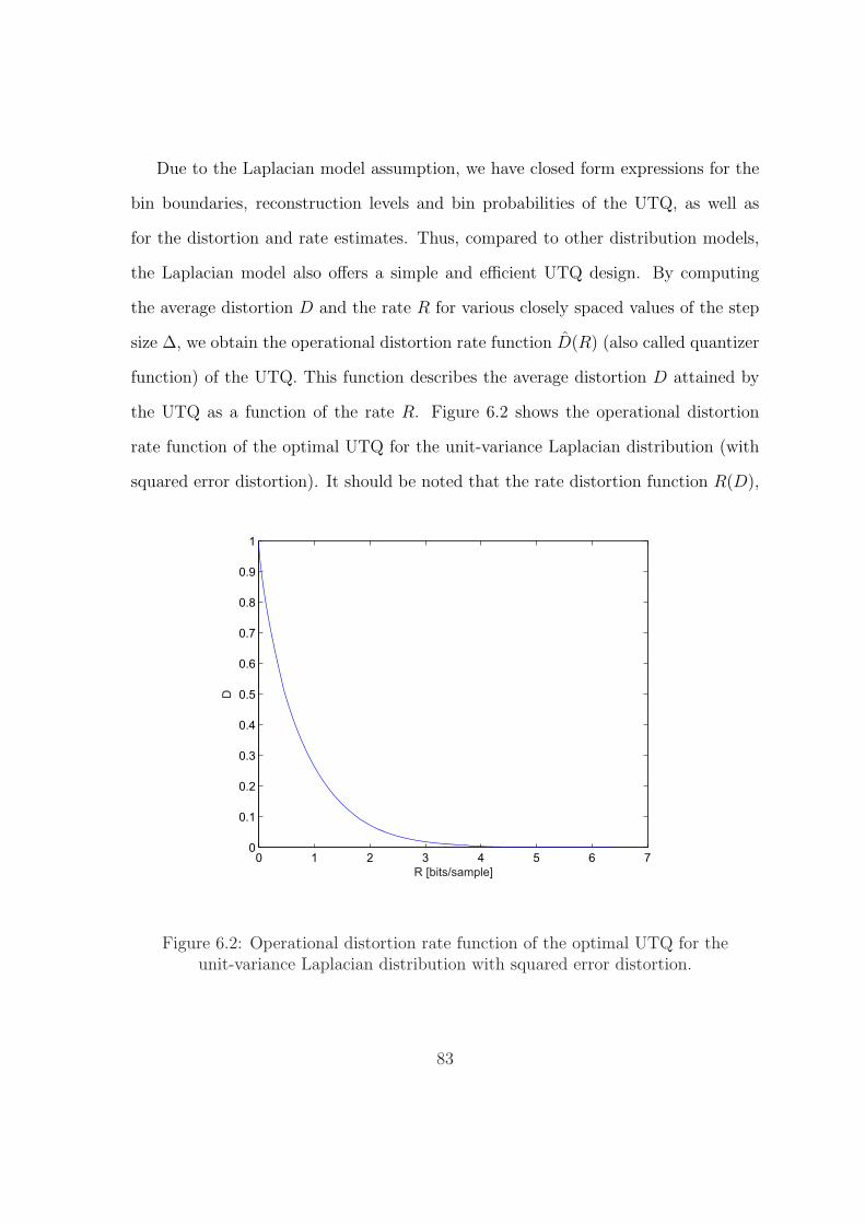
Due to the Laplacian model assumption, we have closed form expressions for the

bin boundaries, reconstruction levels and bin probabilities of the UTQ, as well as

for the distortion and rate estimates. Thus, compared to other distribution models,

the Laplacian model also offers a simple and efficient UTQ design. By computing

the average distortion D and the rate R for various closely spaced values of the step

size Δ, we obtain the operational distortion rate function D(R) (also called quantizer

function) of the UTQ. This function describes the average distortion D attained by

the UTQ as a function of the rate R. Figure 6.2 shows the operational distortion

rate function of the optimal UTQ for the unit-variance Laplacian distribution (with

squared error distortion). It should be noted that the rate distortion function R(D),

0 1 2 3 4 5 6 70

0.1

0.2

0.3

0.4

0.5

0.6

0.7

0.8

0.9

1

R [bits/sample]

D

Figure 6.2: Operational distortion rate function of the optimal UTQ for theunit-variance Laplacian distribution with squared error distortion.

83

or the distortion rate function D(R) [13], for a Laplacian source with squared error

distortion, can be computed numerically using the Blahut-Arimoto algorithm [4, 7, 2],

as done in [53]. For completeness, we also point out that for the case of absolute

difference distortion, i.e., d(x, x) = |x − x|, there exists a closed form expression for

the rate distortion function D(R) for a Laplacian source [4, Ch. 4], [10].

6.2 Uniform Reconstruction with Unity Ratio Quan-

tizers as an Alternative to Uniform Threshold

Quantizers

As described in Section 6.1, the uniform threshold quantizer (UTQ) is used effec-

tively by numerous image subband quantization schemes. Interestingly, another rel-

atively simple and effective quantizer for the Laplacian distribution—the uniform

reconstruction with unity ratio quantizer (URURQ) [53]—is hardly ever used in such

applications. Although the UTQ well approximates the optimum entropy-constrained

scalar quantizer (ECSQ) for the Laplacian distribution (assuming MSE distortion),

the URURQ still offers a small improvement in rate distortion performance, com-

pared to the UTQ [53]. For the proposed MD coder, we also examine the utilization

of URURQs as an alternative to UTQs, to see how this slight performance improve-

ment in theory (i.e., for simulated Laplacian data), translates into practice (i.e., in

terms of the overall performance of the coder, with quantization of real wavelet data).

In this section we provide a brief and concise description of the URURQ.

The URURQ is defined by its step size Δ—the distance between adjacent recon-

struction levels. This is illustrated in Figure 6.3. As described in Section 6.1, we

84

only focus on quantizers with odd number of levels (“mid-tread” quantizers) in order

to be able to obtain low bit rates (i.e., low redundancy), if desired. For Laplacian

x

b1

b2

f(x)

b3

bL

b-L

b-3

b-2

b-1

q1= q

Lq

-Lq

-2q

0q

2=2 q

3=3q

-1q

-3

Figure 6.3: Uniform reconstruction with unity ratio quantizer (URURQ) with stepsize Δ and an odd number of levels N = 2L + 1. The bin boundaries are denoted by

{bj} and the reconstruction levels by {qj}. The Laplacian pdf is also shown forillustration.

distribution with parameter λ, the leftmost bin boundary on the positive half of the

real line is

b1 = Δ − δ(Δ) (6.20)

where

δ(Δ) = arg minψ

{∫ Δ

0

(x − ψ)2e−λx dx

}. (6.21)

Differentiating with respect to ψ and setting to zero to find the minimizer, yields

δ(Δ) =1

λ− Δ

eλΔ − 1(6.22)

which also equals1 δ of (6.16). The URURQ is symmetric, and the rest of the bin

boundaries to the right of b1 essentially construct a uniform threshold sub-quantizer

1This equality is not a coincidence, of course. It is a consequence of the useful property of theLaplacian distribution stated (and proved) in Appendix C.

85

(to the right of b1) with step size Δ. Note that given the bin boundaries, the re-

construction levels of the URURQ satisfy the well-known centroid condition (i.e.,

conditional expectation), and therefore minimize the (MSE) distortion. Also, note

that in [53], the dead-zone ratio z is defined as z = b1/(Δ − δ(Δ)), which equals one

in the case of the URURQ, and reveals the origin of the term “unity ratio” in the

quantizer’s name.

Since the UTQ and the URURQ are very similar and also share many properties in

common, we are able to straightforwardly adapt the proposed MD coder to operate

with URURQs instead of UTQs. Specifically, we adapt all the coding procedures

related to the UTQs also to the case of URURQs. In Appendix E we also derive

a closed form expression for the average squared error distortion D of the URURQ,

whose evaluation does not involve integration. In addition, some experimental results

with URURQs are presented in Chapter 8.

For brevity, in the sequel we generally refer to the quantizers used by the proposed

coder (to quantize the coefficients of the redundant polyphase component of each

description) only as UTQs. Nevertheless, the same guidelines hold for URURQs as

well.

6.3 Optimal Model-Based Bit Allocation

The context-based classification enables the proposed coder to utilize a set of quan-

tizers, each customized to an individual class, for coding the redundant polyphase

component of each description. Define the base rate of a given description as the

average bit rate (in bits/pixel) at which the primary polyphase component of the de-

scription is encoded (using the wavelet coefficients encoder of Figure 4.8). Similarly,

86

define the redundancy rate of the description as the average bit rate (in bits/pixel) at

which the redundant polyphase component of the description is encoded. Note that

here we use the convention that the averaging is with respect to the total number of

image pixels, so that all rates from all descriptions can be summed to produce the to-

tal encoding rate for the image. Given the desired redundancy rate for a description,

the encoder needs to determine the rate at which each of the customized quantizers

operates. To this end, the proposed coder utilizes an optimal model-based bit allo-

cation scheme. This efficient bit allocation scheme is based on variance scaling and

on a pre-designed, indexed array of optimized uniform threshold quantizers (UTQs)

of different step sizes. This array of UTQs is created only once, off-line, and can be

regarded as a fixed resource of the coder, used by both the encoder and the decoder.

It enables the proposed coder to avoid complex on-line bit allocation procedures, as

well as to intelligently and instantly adapt the arithmetic entropy encoder to the

varying coefficients statistics, by storing the pre-computed bin probabilities of each

UTQ. It should be noted that this adaptation scheme enables the entropy encoder to

fully exploit the higher level statistics captured by the Laplacian model-based clas-

sification and quantization algorithms, rather than using ad hoc updating rules, as

done in many other entropy coding adaptation schemes.

The bit allocation, which is based on the Laplacian model, is performed in the

general framework of Lagrangian optimization [40, 50, 55]. It is carried out for each

description separately, given the desired redundancy rate for the description, and

performed over all classes of redundant coefficients from all subbands simultaneously

(for the approximation subband, a predictive, DPCM-like, quantization scheme is

employed, so the prediction errors are considered instead; this will be described in

Section 7.2.1).

87

Given the desired redundancy rate for the description, we wish to find the optimal

rate for each of the different classes (from all subbands), such that the resulting

MSE distortion in the image domain is minimized, subject to the redundancy rate

constraint. As before, we assume that the coefficients in each class are drawn from a

Laplacian distribution (the Laplacian parameter estimate λ for each class is obtained

from the classification thresholds design procedure, as described in Section 5.3).

The following notation is used in the sequel:

D : Average squared error distortion (MSE) in the image domain, resulting from

quantization of coefficients in the redundant polyphase component.

R : Average rate (in bits/pixel) for encoding the coefficients in the redundant polyphase

component (i.e., the redundancy rate of the description).

RT : Desired redundancy rate (in bits/pixel) for the description.

B : The total number of classes (from all subbands).

b : Index of a specific class (1 ≤ b ≤ B).

Nb : Number of coefficients in the class b.

N : Number of pixels in the image.

ηb : The ratio Nb/N , i.e., the ratio between the number of coefficients in the class b

and the number of pixels in the image.

Db : Average squared error distortion (MSE) in the transform domain in encoding

the class b, where the averaging is with respect to the number of coefficients in

the class (Nb).

88

Rb : Average rate (in bits/coefficient) for encoding the coefficients in the class b, where

the averaging is with respect to the number of coefficients in the class (Nb).

Gb : The synthesis (inverse transform) energy gain factor associated with the subband

to which the class b belongs. This energy gain factor represents the amount of

squared error in the synthesized image introduced by a unit error in a transform

coefficient of the subband. For an orthonormal transform Gb = 1,∀b. A detailed

description will be given in Section 7.1.2.

Thus, given the desired redundancy rate RT , our objective is to find the optimal

rates {Rb}Bb=1 for the different classes, such that the distortion D is minimized, subject

to the constraint R ≤ RT . We use Lagrangian optimization [40, 50, 55] to solve this

constrained optimization problem, and instead seek to minimize the Lagrangian cost

function

J(ξ) = D + ξR (6.23)

for a fixed Lagrange multiplier ξ. Later, we will describe how to determine the

Lagrange multiplier ξ such that R = RT (or, more precisely, R ∈ (RT − ε, RT ] for an

arbitrary tolerance ε > 0). This will also yield the solution to the original constrained

optimization problem [50].

The average distortion and rate are given by

D =B∑

b=1

ηbGbDb(Rb) (6.24)

and

R =B∑

b=1

ηbRb , (6.25)

89

respectively. Thus,

minR1,...,RB

J(ξ) = minR1,...,RB

{D + ξR} =

= minR1,...,RB

{B∑

b=1

ηbGbDb(Rb) + ξ

B∑b=1

ηbRb

}=

=B∑

b=1

minRb

{ηbGbDb(Rb) + ξηbRb} =

=B∑

b=1

ηb minRb

{GbDb(Rb) + ξRb} (6.26)

which suggests that the minimum can be computed independently for each class.

For a given class b, the optimal rate Rb which minimizes

GbDb(Rb) + ξRb (6.27)

can be found by differentiating (6.27) with respect to Rb and setting to zero. This

yields

GbD′b(Rb) + ξ = 0 , (6.28)

or

D′b(Rb) = − ξ

Gb

, (6.29)

where D′b(Rb) is the derivative of the distortion Db, evaluated at Rb bits/coefficient.

The rates {Rb}Bb=1 are thus chosen to satisfy the following rate allocation equations

D′b(Rb) = − ξ

Gb

, b = 1, . . . , B . (6.30)

For each class, the relevant equation specifies the required slope on the operational

distortion rate function of the corresponding UTQ (and thus determines its step

size). The rate allocation equations (6.30) realize the well-known “constant slope”

principle [40] in Lagrangian optimization, adapted to the case of a non-orthonormal

transform (i.e., arbitrary Gb’s).

90

For efficiency, our bit allocation scheme utilizes the following properties of the

optimal UTQ for the Laplacian distribution, optimized for minimum MSE distortion:

1. For a given rate (output entropy), the optimal quantizer for an input with

variance σ2 is a scaled version, by σ, of the optimal quantizer for a unit-variance

input (i.e., the bin boundaries and reconstruction levels of the unit-variance

quantizer are to be multiplied by σ). The bin probabilities (and obviously the

output entropy) of both quantizers are the same.

2. The distortion attained by the scaled quantizer above is larger by a factor

of σ2 compared to that attained by the unit-variance quantizer (each with its

corresponding input).

These properties can be easily proved using the definitions and computations of Sec-

tion 6.1. The important consequence of the aforementioned properties is that the

operational distortion rate function D(R) of the optimal UTQ for an input with vari-

ance σ2 can be obtained from the normalized distortion rate function (i.e., that for a

unit-variance input; see Figure 6.2) by merely scaling the distortion axis by σ2. Ob-

viously, the slope (the derivative of the distortion with respect to the rate) is affected

similarly (i.e., multiplied by a factor of σ2).

Thus, in order to solve the rate allocation equations (6.30), we can avoid comput-

ing the operational distortion rate function of the optimal UTQ of each class b (for

the class-specific Laplacian parameter estimate λb, or variance estimate σ2b = 2/λ2

b).

Instead, we only compute (off-line) the operational distortion rate function of the

UTQ for the unit-variance Laplacian distribution, and infer the required operating

point of the UTQ of each class b from that normalized distortion rate function and

the normalized slope −ξ/(Gbσ2b ), as detailed next.

91

Off-line, we create an array of optimized UTQs for the unit-variance Laplacian

distribution, where each quantizer has a different step size Δ. For each quantizer, we

compute and store the bin boundaries, reconstruction levels, and bin probabilities,

as well as the resulting rate and distortion, as detailed in Section 6.1. By using

closely spaced values of the step size Δ, we also obtain the operational distortion

rate function of the optimal UTQ for the unit-variance Laplacian distribution, and

are able to well approximate its derivative (i.e., slope) at each operating point. For

each quantizer in the array we also store the corresponding slope on the operational

distortion rate function, which enables us to index the array by the slope (as required

by the bit allocation algorithm).

During the encoding process itself, for a fixed Lagrangian multiplier ξ, and a given

class b, we need to choose the appropriate quantizer (in order to quantize the coeffi-

cients of the class b). To do so, we first translate the (non-normalized) slope −ξ/Gb

from the relevant rate allocation equation of (6.30) to the corresponding normal-

ized slope −ξ/(Gbσ2b ) on the unit-variance operational distortion rate function, where

σ2b = 2/λ2

b is the variance estimate for the class b. Since the pre-computed array of

optimized UTQs is indexed by the slope, the appropriate “normalized” quantizer (i.e.,

the one whose slope is closest to the required normalized slope) can be instantly ob-

tained from the array. The actual quantizer for the class b is simply the scaled version,

by σb, of this “normalized” quantizer, as explained earlier in this section. Namely,

the bin boundaries and reconstruction levels are multiplied by σb, while the bin prob-

abilities remain unchanged. The bin probabilities are also used to instantly adapt the

arithmetic entropy encoder that follows the quantization stage to the statistics of the

class b, as captured by the model-based classification algorithm.

We now turn to describe how to determine the Lagrange multiplier ξ in the

92

Lagrangian cost function J(ξ) of (6.23), such that R = RT (or, more precisely,

R ∈ (RT − ε, RT ] for an arbitrary tolerance ε > 0). First, define the following

function

f(ξ) = R(ξ) − RT (6.31)

where RT is the desired redundancy rate, and R(ξ) is the average redundancy rate

resulting from minimization of the Lagrangian cost function of (6.23) (for the same

Lagrange multiplier ξ). Finding a proper ξ such that R(ξ) = RT is then equivalent

to finding a root of f(ξ). Since R(ξ) is monotonically non-increasing with ξ [50] (as ξ

controls the penalty for an increased rate in the Lagrangian cost function of (6.23)),

root finding of f(ξ) can be easily performed using the bisection method [42, Ch. 9].

This involves bracketing a root (i.e., finding ξ1 and ξ2 such that f(ξ1) > 0 and

f(ξ2) < 0), and then iterating until R(ξ) ∈ (RT − ε, RT ], for an arbitrary tolerance

ε > 0 (e.g., ε = 0.005).

The resulting value of ξ, which specifies the bit allocation, is also transmitted to

the decoder (as part of the side information for the description). For each class in

each subband, the decoder can then match the same UTQ used by the encoder, by

repeating the aforementioned variance scaling procedure performed by the encoder.

The bin probabilities of the matched UTQs serve to properly adapt the arithmetic

entropy decoder, and the classification and dequantization stages follow to correctly

decode the redundant polyphase component of the description. Obviously, decoding

this redundant part of information is needed only in the case that the other description

is lost, as explained in Section 4.2.

93

Chapter 7



Implementation Considerations

and Miscellaneous

7.1 Implementation Considerations

7.1.1 Boundary Extension for Wavelet Transform

Section 4.1.1 described the computation of the two-dimensional discrete wavelet trans-

form of an image using a series of filtering (and downsampling) operations. Since the

image and the filters are of finite length, special attention has to be paid in com-

puting their convolution, at each stage of the decomposition process. This section

addresses the problem of boundary extension for the wavelet transform, especially

94

referring to coding applications. In order to simplify the discussion, some of the con-

cepts in this section are illustrated using the one-dimensional wavelet transform, but

hold equally well for the two-dimensional case (through the separable extension of

the one-dimensional transform, as described in Section 4.1.1).

As detailed in [57], the standard orthogonal wavelet transform [51, Ch. 6] has a

significant shortcoming that limits its usefulness in coding applications: it generally

results in “coefficient expansion”, that is to say, the number of output wavelet coef-

ficients is greater than the number of input samples. This increase in the number of

coefficients generally degrades the performance of the coding system, since extra bits

are required to represent the additional coefficients. This is the case, for example, if

zero-padding boundary extension is used, which assumes that the image is zero out-

side its boundaries. Zero-padding extension may also result in unpleasant artifacts,

usually in the form of dark areas, near the boundaries of the reconstructed image.

Coefficient expansion can be eliminated by using periodic-padding boundary ex-

tension (or circular convolution), which assumes that the image is periodic. This type

of extension generally results in large discontinuities near the boundaries, however,

and extra bits are required in order to code them. Moreover, annoying artifacts near

the boundaries of the reconstructed image may appear due to quantization of the

artificially introduced large wavelet coefficients at the locations of the discontinuities.

An effective way to avoid coefficient expansion and greatly reduce boundary ar-

tifacts is to use symmetric (or antisymmetric) wavelet filters along with symmetric

boundary extension. By using symmetric boundary extension, the image is extended

in a continuous way outside its boundaries, and thus artificial discontinuities are

avoided. Due to the symmetry imposed by the extension, there is virtually no ef-

fective increase in the number of input samples, and coefficient expansion can be

95

avoided if the symmetry is preserved at each stage of the decomposition process. The

key underlying concept is that the convolution of a symmetric (“linear phase”) input

with a linear phase filter produces a linear phase output (this can be easily observed

in the frequency domain as the linear exponents add and remain linear), and that the

exact type of symmetric extension can be chosen such that the symmetry is preserved

also by the downsampling operation.

Two types of symmetric extension should be considered in this context—half-

point and whole-point symmetric extension—where the former repeats the outermost

samples of the input, while the latter does not. This is illustrated in Figure 7.1. As

0 1 2 3 4 5 6 70

1

2

3

4

5

(a)

0 1 2 3 4 50

1

2

3

4

5

(b)

Figure 7.1: Half-point and whole-point symmetric extensions. (a) Half-pointsymmetric extension. (b) Whole-point symmetric extension. The original

(one-dimensional) input is shown in blue, and the extension is shown in red. Theresulting axes of symmetry are shown in black, and are located at “half-point”

locations in (a) and at “whole-point” locations in (b). One period of the extendedinput is shown in solid lines.

shown, the extended input is periodic for either type of extension. For an input of

length L, the period of the extended input is 2L in the case of half-point symmetric

96

extension, and is 2(L − 1) in the case of whole-point symmetric extension. In both

cases, however, only L samples of the extended input are not redundant.

Two questions still have to be answered: First, are there any linear phase (i.e.,

symmetric or antisymmetric) wavelet filters? And second, can we guarantee that the

downsampling operation will preserve the symmetry by choosing the proper type of

symmetric extension?

Regarding the first question, unfortunately, for real valued, compactly supported

orthogonal wavelets, the only set of linear phase filters is the trivial set of Haar fil-

ters [14]. Nevertheless, the more general form of biorthogonal wavelets [51, Ch. 6]

permits the use of a much broader class of filters, which includes more sophisticated

linear phase filters, and has been shown to provide an improved performance (com-

pared to the use of orthogonal wavelets) in image coding applications [35]. It should

be noted that unlike the orthonormal wavelet transform, the biorthogonal wavelet

transform does not possess the useful property of being energy preserving, as will be

discussed in Section 7.1.2.

We now give an answer to the second question, dealing with choosing the proper

type of symmetric extension (half-point or whole-point) such that the symmetry can

be preserved by the downsampling operation. The proper type of extension is re-

lated to the lengths of the wavelet filters used, and the following guideline should be

followed:

• Use a half-point (repeat) symmetric extension for an even-length filter.

• Use a whole-point (no repeat) symmetric extension for an odd-length filter.

The various tricky details involved in deriving the above guideline, as well as detailed

directions for proper downsampling of the symmetric output of the filters, are given

97

in [51, Ch. 8].

In summary, coefficient expansion and unpleasant boundary artifacts can be avoided

by using linear phase wavelet filters along with symmetric boundary extension. De-

pending on the lengths of the filters used, the proper type of extension (half-point or

whole-point) should be chosen. The specific choice of wavelet filters and boundary

extension for the proposed MD coder will be detailed in Chapter 8. The consequences

of using the non-energy preserving biorthogonal wavelet transform, which enables the

use of efficient linear phase filters, are addressed next.

7.1.2 Optimal Bit Allocation for Biorthogonal Wavelet Trans-

form

As discussed in the previous section, biorthogonal wavelets permit the use of a much

broader class of filters, compared to orthogonal wavelets, which includes non-trivial

linear phase filters. Nevertheless, one of the main drawbacks of the biorthogonal

wavelet transform is that, unlike the orthonormal wavelet transform, it does not

possess the useful property of being energy preserving. Therefore, bit allocation algo-

rithms which are optimal for energy preserving transforms (e.g., orthonormal wavelet

transform), are no longer optimal in the case of biorthogonal wavelet transform. Yet,

numerous coding systems that utilize biorthogonal wavelets, use bit allocation pro-

cedures that were designed for orthonormal wavelets, although these bit allocation

procedures provide suboptimal performance, in terms of distortion versus rate, in the

case of biorthogonal wavelets [8].

This section discusses optimal bit allocation for biorthogonal wavelet transform,

and provides a procedure to adapt standard bit allocation algorithms to this special

98

case. The adaptation is based on the fact that the biorthogonal transform essentially

weights the MSE in each of the subbands to obtain the MSE in the reconstructed

output, according to the energy expansion properties of the synthesis system (inverse

transform), under the assumption that the quantization errors are uncorrelated, with

zero mean [56]. Using the notation of Section 6.3, the MSE in the reconstructed

image can therefore be presented as a weighted average of the MSEs in the different

subbands, as in (6.24), to obtain

D =∑

b

ηbGbDb(Rb) (7.1)

where the Gb’s are the synthesis energy gain factors (weights) associated with the

different subbands1. For an orthonormal transform Gb = 1, ∀b. It should be noted

that although our discussion is generally oriented towards the two-dimensional case

(i.e., towards image coding), the principles presented also apply to other cases.

The energy gain factor Gb of a given subband represents the amount of squared

error in the reconstructed image introduced by a unit error in a transform coefficient

of the subband. It can be shown that this energy gain factor is given by the squared

l2 norm (energy) of the synthesis basis vectors for this subband [55, Ch. 4].

Computation of the energy gain factor of a subband given the synthesis filters can

be performed by computing the squared l2 norm of the single equivalent filter which

takes the subband coefficients directly to the reconstructed output [57]. Specifically,

in the case of a two-dimensional separable wavelet transform, the energy gain factor

of a subband is the product of its “vertical weight” and its “horizontal weight”. The

vertical (horizontal) weight of a subband is related to the synthesis filters applied

in the vertical (horizontal) dimension during the synthesis from the subband to the

1In the notation of Section 6.3, a single class in each subband is assumed here.

99

reconstructed image. As an example, coefficients belonging to the horizontal detail

subband at level three of the wavelet transform (dH3 ), undergo one highpass filtering

operation followed by two lowpass filtering operations in the vertical dimension dur-

ing the synthesis, and three lowpass filtering operations in the horizontal dimension.

Denote the impulse responses of the one-dimensional lowpass and highpass synthesis

filters by lr and hr, respectively. The vertical weight is computed by first upsampling

hr by a factor of two (i.e., adding one zero between each coefficient in hr) and convolv-

ing the result with lr. The result of the convolution is then upsampled by a factor of

two and convolved with lr. The vertical weight is given by the squared l2 norm (i.e.,

the sum of squares) of the final convolution result. The horizontal weight is computed

in a similar manner, using lr three times. The product of the vertical and horizontal

weights then gives the energy gain factor of the subband under discussion (dH3 ).

As an example, consider the Cohen-Daubechies-Feauveau (CDF) biorthogonal

wavelet transform using 9/7-tap wavelet filters [11, 1], extensively utilized in im-

age compression applications. Using the above procedure, we computed the energy

gain factors of the various subbands of the corresponding three-level two-dimensional

wavelet decomposition. The obtained energy gain factors are shown in Table 7.1. As

can be seen, the energy gain factors are not equal to one, suggesting that the trans-

form is not energy preserving. Nevertheless, the energy gain factors for this particular

transform deviate only by a few percent from one, implying that the transform is rea-

sonably “close” to being orthogonal. Other biorthogonal transforms may generally

present much higher deviations from orthogonality, which must be taken into consid-

eration by the bit allocation algorithm of a coding system utilizing the biorthogonal

wavelet transform, in order to achieve optimal performance for the system.

100

Level Subband Energy Gain Factor

dD1 (Diag. details) 1.08250699475332

1 dV1 (Vert. details) 1.02270033578441

dH1 (Horiz. details) 1.02270033578441

dD2 (Diag. details) 0.93550641543575

2 dV2 (Vert. details) 0.99681499726207

dH2 (Horiz. details) 0.99681499726207

dD3 (Diag. details) 1.08082593648928

3 dV3 (Vert. details) 1.09378514093722

dH3 (Horiz. details) 1.09378514093722

a3 (Approximation) 1.10689972746311

Table 7.1: Energy gain factors for the three-level two-dimensional biorthogonalwavelet transform using Cohen-Daubechies-Feauveau (CDF) 9/7-tap wavelet filters.

7.2 Miscellaneous

7.2.1 Prediction Scheme for Approximation Coefficients

In the proposed context-based MD encoder (see Figure 4.8 in Section 4.2), the various

components in the encoding path of the redundant polyphase component of each de-

scription model the detail wavelet coefficients (i.e., the coefficients from all subbands

excluding the approximation) using a (zero-mean) Laplacian distribution. For the

approximation subband, a prediction scheme is employed first, based on quantized

approximation coefficients of the complementary polyphase component, and the re-

sulting prediction errors are then encoded. Since the prediction errors are modeled

using the same Laplacian distribution model used for the detail coefficients, the same

encoding scheme can be utilized for all subbands (where for the approximation sub-

band the prediction errors are encoded).

The prediction scheme employed for the approximation subband predicts the value

101

of each approximation coefficient in the redundant polyphase component based on

quantized neighboring coefficients of the complementary polyphase component. This

is shown in Figure 7.2. (Notice the resemblance to contexts formed for context-based

classification.) The predicted value for the approximation coefficient Xi,j is given by

Xi+1,j-1

Xi-1,j-1

Xi,j

Xi-1,j

Xi-1,j+1

Xi+1,j

Xi+1,j+1



Figure 7.2: Prediction of an approximation coefficient Xi,j based on its quantizedneighbors. The approximation coefficient Xi,j belongs to the redundant polyphase

component, and is shown in black. The quantized coefficients used for theprediction belong to the primary polyphase component, and are shown in white.

a weighted average of its quantized neighbors shown. The proposed coder uses the

following prediction mask

1

2(1 +

√2) ·

1√2

1 1√2

·1√2

1 1√2

(7.2)

102

so that the weights are inversely proportional to the Euclidean distances of the cor-

responding quantized neighbors from the coefficient Xi,j , and sum to one. The pre-

diction error is then given by the difference between Xi,j and its predicted value.

The context-based classification of the prediction errors (corresponding to approx-

imation coefficients of the redundant polyphase component) is performed in a very

similar manner to that performed for detail coefficients. The distinction is that, in-

stead of being based on magnitudes of neighboring quantized coefficients from the

primary polyphase component of the description, the classification procedure in the

approximation subband is based on magnitudes of generated “prediction errors”, com-

puted using quantized approximation coefficients of the primary polyphase compo-

nent. Note that these generated prediction errors are neither encoded nor transmitted

in any way, but only serve to provide contextual information for the classification of

the actual prediction errors (corresponding to approximation coefficients of the re-

dundant polyphase component). The underlying assumption is that large prediction

errors in the approximation subband tend to cluster together at relatively active ar-

eas (e.g., edges), and that these dependencies can be utilized to efficiently encode the

prediction errors to be transmitted. Thus, for the approximation coefficients of the

redundant polyphase component, contexts are formed from generated prediction er-

rors, computed using quantized approximation coefficients of the primary polyphase

component. Specifically, instead of using the context coefficients shown in Figure 5.1

themselves, each coefficient in the context is replaced by its corresponding gener-

ated prediction error. This generated prediction error is calculated as the difference

between the quantized context coefficient (belonging to the primary polyphase com-

ponent) and a weighted average of three of its quantized neighbors (which also belong

103

to the primary polyphase component). For illustration, see Figure 7.3, which resem-

bles Figure 5.1, but also marks with asterisks the three neighboring coefficients used

to “predict” the value of the quantized approximation coefficient Xi−1,j−1. In the

Xi+1,j-1

Xi-1,j-1*

* *

Xi,j

Xi-1,j

Xi-1,j+1

Xi+1,j

Xi+1,j+1



Figure 7.3: Quantized coefficients from the primary polyphase component (markedwith asterisks) used to “predict” the value of the quantized approximation

coefficient Xi−1,j−1.

formation of the context for the classification of the actual prediction error of Xi,j,

the context coefficient Xi−1,j−1 is replaced by the difference between its (quantized)

value and a weighted average of its three quantized neighbors marked with asterisks.

The weights in the above weighted average can be chosen, for example, to correspond

to the following weighting mask [19, Ch. 8]

-0.5 0.75

0.75 ·

(7.3)

whose elements sum to one. The rest of the context is formed in a similar manner,

104

with the required spatial adjustments. The context-based classification procedure for

the prediction errors corresponding to approximation coefficients of the redundant

polyphase component, given the contexts formed from generated “prediction errors”,

is identical to that used for the detail coefficients (described in Chapter 5).

Finally, we note that some standard (single description) wavelet coders employ

a predictive (DPCM-like) quantization scheme for the approximation wavelet coef-

ficients, and encode the resulting quantized prediction errors. If such a coder is

utilized in the proposed MD coding scheme (as the “wavelet coefficients encoder” in

Figure 4.8) to encode the primary polyphase component of each description, these

quantized prediction errors can directly replace the aforementioned generated “pre-

diction errors”, and provide the contextual information for the classification of the

actual prediction errors (corresponding to approximation coefficients of the redundant

polyphase component). Obviously, in such a case, there is no need to explicitly gener-

ate the aforementioned “prediction errors” in order to provide the required contextual

information.

105

Chapter 8

Experimental Results

This chapter provides experimental results obtained by the proposed context-based

MD wavelet image coding system. We begin with a detailed description of the actual

configuration of the system used to produce the results. Demonstrations related to

the quality of the context-based classification follow, as well as both objective and

subjective performance results, which also include a comparison to other relevant

MD image coding systems. In addition, the effect of various choices made by the

system on the resulting performance is presented and analyzed. We then demonstrate

the improvement in coding efficiency due to the effective utilization of contextual

information, which we refer to as the context gain. Finally, we describe how to

determine the optimal operating point for the proposed MD coder, based on the

properties of the communication channel.

106

8.1 System Configuration

A simplified block diagram of the proposed context-based MD encoder was presented

in Figure 4.8 (in Section 4.2). Referring to the block diagram shown, this section

provides a detailed description of the actual configuration of the various components

of the system, as used to produce the experimental results presented in the chapter.

Regarding the choice of wavelet transform, we avoid coefficient expansion and

unpleasant boundary artifacts by utilizing linear phase wavelet filters along with

symmetric boundary extension, as discussed in Section 7.1.1. Specifically, a two-

dimensional biorthogonal wavelet transform using Cohen-Daubechies-Feauveau (CDF)

9/7-tap wavelet filters [11, 1] is employed, a choice which has been shown experimen-

tally to provide excellent performance for image compression [64]. Since the wavelet

filters are of odd length, a whole-point (no repeat) symmetric boundary extension

is used, and coefficient expansion is avoided (see Section 7.1.1). The number of lev-

els in the decomposition is set to three, and the resulting number of subbands is

therefore 10.

The polyphase transform used by the proposed coder is the plain polyphase trans-

form, which, for each column (or row) in each subband, simply groups all the odd-

numbered coefficients into one polyphase component and all the even-numbered coef-

ficients into the other component. This is shown in Figure 8.1. The orientation of the

polyphase transform is adapted to the orientation of the subband on a subband-by-

subband basis, in order to enable the context-based classification procedure to more

effectively utilize of the contextual information extracted from the complementary

polyphase component. Thus, for all subbands except those of horizontal details the

polyphase transform shown in Figure 8.1 is used, while for subbands of horizontal

107

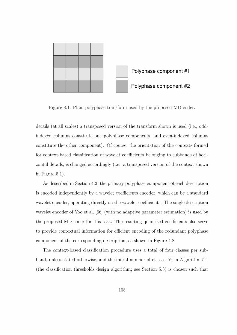
Polyphase component #1

Polyphase component #2

Figure 8.1: Plain polyphase transform used by the proposed MD coder.

details (at all scales) a transposed version of the transform shown is used (i.e., odd-

indexed columns constitute one polyphase components, and even-indexed columns

constitute the other component). Of course, the orientation of the contexts formed

for context-based classification of wavelet coefficients belonging to subbands of hori-

zontal details, is changed accordingly (i.e., a transposed version of the context shown

in Figure 5.1).

As described in Section 4.2, the primary polyphase component of each description

is encoded independently by a wavelet coefficients encoder, which can be a standard

wavelet encoder, operating directly on the wavelet coefficients. The single description

wavelet encoder of Yoo et al. [66] (with no adaptive parameter estimation) is used by

the proposed MD coder for this task. The resulting quantized coefficients also serve

to provide contextual information for efficient encoding of the redundant polyphase

component of the corresponding description, as shown in Figure 4.8.

The context-based classification procedure uses a total of four classes per sub-

band, unless stated otherwise, and the initial number of classes N0 in Algorithm 5.1

(the classification thresholds design algorithm; see Section 5.3) is chosen such that

108

each class initially contains approximately 16 coefficients. This choice for the initial

number of classes offers a relatively dense set of initial thresholds (from which the

final thresholds are selected), and yet enables a reliable estimation of the Laplacian

parameter for each class. We experimentally found this choice to yield very good

classification results, compared to other choices.

For each description, the resulting classification thresholds and Laplacian param-

eter estimates (for each of the subbands) are transmitted to the decoder as side

information. The side information for each description also includes the value of the

Lagrange multiplier ξ, which specifies the bit allocation (see Section 6.3). Each of

the side information parameters is represented using 16 bits (in fixed-point represen-

tation). Note that the resulting overhead due to the side information is generally

minimal. For example, for the various choices stated above, the overhead due to side

information translates to an excess rate of less than 0.004 bpp (bits per pixel), per

description, in the case of a grayscale input image of size 512 × 512 pixels.

Finally, we note that we consider in our experiments the balanced MD coding

scenario, in which the generated descriptions are of statistically equal rate and impor-

tance. This balanced case is generally the one considered in MD coding applications,

as it is well matched to communication systems with no priority mechanisms for data

delivery (e.g., the Internet) [30].

8.2 Quality of Classification

This section demonstrates the subjective quality of the context-based classification,

which enables the proposed MD coder to efficiently encode the redundant polyphase

component of each description, based on quantized coefficients of the complementary

109

polyphase component.

As an example, consider the original (grayscale) image Lena, of size 512 × 512

pixels, shown in Figure 8.2(a). The wavelet transform (in absolute value) of the im-

(a) (b)

Figure 8.2: Original images (grayscale) of size 512 × 512 pixels.(a) Lena. (b) Goldhill.

age Lena, with approximation coefficients replaced by their corresponding prediction

errors (see Section 7.2.1), is shown in Figure 8.3(a). Note that all subbands have been

enhanced to make their underlying structure more visible. Figure 8.3(b) shows the

corresponding classification map, where the classification of each coefficient is based

on quantized coefficients from the complementary polyphase component (in this ex-

ample the quantization of the primary polyphase component of each description is at

an average rate of 0.48 bpp, per description). This classification map has only four

gray levels, corresponding to the four possible classes in each subband (coefficients

110

(a) (b)

Figure 8.3: (a) Wavelet transform (in absolute value) of the original image Lena,with approximation coefficients replaced by their corresponding prediction errors.

(b) Corresponding classification map (with four gray levels).

111

assigned to the least active class C0 are shown in black, and those assigned to the most

active class C3 are shown in white). As shown, despite the fact that the classification

of each coefficient is based solely on quantized neighboring coefficients from the com-

plementary polyphase component, areas with different energy levels are successfully

identified by the context-based classification procedure, and effective classification is

achieved.

Figure 8.4 shows the histograms corresponding to the four classes assigned to the

coefficients in subband dH1 of the redundant polyphase component of description 1.

Each of the histograms shows the actual distribution of the coefficients assigned to its

corresponding class, and also includes a plot of the fitted Laplacian pdf for the class

(using maximum likelihood estimation of the Laplacian parameter, as described in

Section 5.3). As shown, the classified coefficients are successfully separated into four

different classes according to their activity, where classes corresponding to a higher

activity indeed contain coefficients with a larger variance. In addition, the Laplacian

pdf matched to the coefficients in each class fits their actual distribution reasonably

well.

8.3 Performance of the System

This section provides both objective and subjective performance results for the pro-

posed MD coder, including a comparison to other relevant MD coding systems. It

also presents and analyzes the effect of various choices made by the system on the

resulting performance.

The PSNR (Peak Signal-to-Noise Ratio) values corresponding to the central and

112

−50 −40 −30 −20 −10 0 10 20 30 40 500

0.2

0.4C0

−50 −40 −30 −20 −10 0 10 20 30 40 500

0.1

0.2C1

−50 −40 −30 −20 −10 0 10 20 30 40 500

0.05

0.1C2

−50 −40 −30 −20 −10 0 10 20 30 40 500

0.05

0.1C3

Figure 8.4: Histograms corresponding to the four classes assigned to the coefficientsin subband dH

1 of the redundant polyphase component of description 1. Eachhistogram also includes a plot of the fitted Laplacian pdf for the class.

113

(average) side distortions attained for different amounts of redundancy for the im-

ages Lena and Goldhill (shown in Figure 8.2) are shown in Figure 8.5 and Figure 8.6,

respectively. The total rate, which takes into account both descriptions altogether,

including the overhead due to side information (i.e., every single bit transmitted) is

fixed, and is set to 1 bpp in this example. Each performance curve is virtually a

29 30 31 32 33 34 35 36 37 3836.5

37

37.5

38

38.5

39

39.5

40

40.5

Side PSNR [dB]

Cen

tral P

SN

R [d

B]

ρ = 0.05 bppρ = 0.07 bpp

ρ = 0.08 bpp

ρ = 0.12 bpp

ρ = 0.15 bpp

ρ = 0.19 bpp

ρ = 0.23 bpp

ρ = 0.28 bpp

ρ = 0.34 bpp

ρ = 0.39 bpp

ρ = 0.46 bpp

Figure 8.5: Performance of the proposed MD coder for the image Lena (total rateof 1 bpp). Also shown is the redundancy rate ρ corresponding to various points on

the performance curve.

parametric curve, where different points on the curve correspond to different amounts

114

26 27 28 29 30 31 32 33 3433

33.5

34

34.5

35

35.5

36

36.5

37

Side PSNR [dB]

Cen

tral P

SN

R [d

B]

ρ = 0.03 bppρ = 0.04 bpp

ρ = 0.07 bpp

ρ = 0.11 bpp

ρ = 0.18 bpp

ρ = 0.24 bpp

ρ = 0.30 bpp

ρ = 0.35 bpp

ρ = 0.40 bpp

ρ = 0.43 bpp

ρ = 0.47 bpp

Figure 8.6: Performance of the proposed MD coder for the image Goldhill (totalrate of 1 bpp). Also shown is the redundancy rate ρ corresponding to various points

on the performance curve.

115

of redundancy (i.e., the rate dedicated for encoding the redundant polyphase compo-

nents in both descriptions), for a fixed total rate (which also includes the redundancy

rate, obviously). Each figure also shows the redundancy rate ρ corresponding to var-

ious points on the performance curve presented. As shown, for a fixed total rate,

increasing the redundancy rate significantly improves the quality of the side recon-

structions (i.e., yields higher side PSNR, or lower side distortion), at the expense of

an increasingly degraded central reconstruction (i.e., lower central PSNR, or higher

central distortion). Obviously, one also has to consider the relative importance of the

side reconstructions, compared to that of the central reconstruction, which is generally

related to the probability of channel failure (i.e., lost description). Thus, determining

the optimal operating point for the system, namely, the optimal amount of redun-

dancy for a fixed total rate, should be based on the properties of the communication

channel. This will be described in Section 8.5.

Recall that our proposed MD coder aims to improve the performance of the orig-

inal polyphase transform-based coding scheme of Jiang and Ortega [30], by utilizing

the special statistical properties of the wavelet decomposition to improve the cod-

ing efficiency of the redundant polyphase component of each description (see Sec-

tion 4.2). In other words, for a given quality of central reconstruction, the proposed

coder aims to provide improved side reconstructions. As an example, Figure 8.7 shows

the performance of the proposed coder, compared to that of the original polyphase

transform-based coder, utilizing either the plain polyphase transform or the vector-

form polyphase transform (see Section 3.2), for the image Lena and a total rate of 1

bpp. As shown, the proposed coder indeed attains improved side reconstructions (i.e,

higher side PSNR), for a given quality of central reconstruction, across the entire

redundancy range. We will see in Section 8.4 that this improvement is due to the

116

29 30 31 32 33 34 35 36 37 3836.5

37

37.5

38

38.5

39

39.5

40

40.5

Side PSNR [dB]

Cen

tral P

SN

R [d

B]

Proposed coderPolyphase (plain)Polyphase (vector−form)

Figure 8.7: Performance of the proposed MD coder (in black), compared to that ofthe original polyphase transform-based MD coder [30], utilizing either the plainpolyphase transform or the vector-form polyphase transform (for the image Lena

and a total rate of 1 bpp).

117

effective utilization of contextual information, obtained from quantized wavelet coef-

ficients of the primary polyphase component of each description, for improving the

coding efficiency of the corresponding redundant polyphase component.

Figures 8.8 and 8.9 illustrate the subjective performance results obtained by the

proposed MD coder, and also demonstrate the possible tradeoff offered by MD coding,

compared to single description (SD) coding. Figure 8.8(a) shows again the original

image Goldhill of size 512 × 512 pixels, which can be compressed, for example, to a

rate of 1 bpp by a JPEG2000 coder1 [55]—a state of the art SD wavelet coder—to

yield a relatively high quality reconstructed image (PSNR of 36.27 dB), as shown in

Figure 8.8(b). However, if two separate bitstreams (“descriptions”) need to be created

and transmitted, with the possibility that one of them will be lost, this SD coder does

not offer a straightforward way to tradeoff the quality of the reconstruction from both

bitstreams with that of the reconstruction from either bitstream alone. Obviously,

as an MD coder, the proposed coder does offer such a tradeoff. For example, for

the same total rate of 1 bpp, with a redundancy rate of 0.47 bpp (and two balanced

descriptions), the proposed MD coder yields a good quality reconstruction from both

descriptions (central PSNR of 33.38 dB), as shown in Figure 8.8(c), as well as from a

single description (side PSNR of 33.26 dB), as shown in Figure 8.8(d).

Figure 8.9 shows a similar illustration for the image Lena of size 512× 512 pixels

(shown again in Figure 8.9(a)). In this case, for an encoding rate of 1 bpp, the

JPEG2000 coder attains a PSNR of 40.03 dB (see Figure 8.9(b)). For the same total

rate of 1 bpp, with a redundancy rate of 0.46 bpp, for example, the proposed MD

coder attains a central PSNR of 37.38 dB (see Figure 8.9(c)), and an average side

1JPEG2000 compression results obtained using Adobe R© Photoshop R© CS2, with Adobe R©

JPEG2000 Plug-in v1.6.

118

(a) (b)

(c) (d)

Figure 8.8: Subjective performance results for the proposed MD coder, also incomparison to SD coding (for the image Goldhill). (a) Original image Goldhill. (b)Reconstructed using JPEG2000 (SD) coder (rate 1 bpp). (c) Central reconstruction

by the proposed coder (total rate 1 bpp, redundancy rate 0.47 bpp). (d) Sidereconstruction by the proposed coder (total rate 1 bpp, redundancy rate 0.47 bpp).

119

(a) (b)

(c) (d)

Figure 8.9: Subjective performance results for the proposed MD coder, also incomparison to SD coding (for the image Lena). (a) Original image Lena. (b)

Reconstructed using JPEG2000 (SD) coder (rate 1 bpp). (c) Central reconstructionby the proposed coder (total rate 1 bpp, redundancy rate 0.46 bpp). (d) Side

reconstruction by the proposed coder (total rate 1 bpp, redundancy rate 0.46 bpp).

120

PSNR of 37.26 dB (see Figure 8.9(d)).

In order to demonstrate the effect of the number of classes used by the context-

based classification procedure on the performance of the proposed coder, Figure 8.10

shows the performance obtained by the coder for various choices of the total number

of classes per subband (for the image Lena and a total rate of 1 bpp). As shown, the

29 30 31 32 33 34 35 36 37 3837

37.5

38

38.5

39

39.5

40

40.5

Side PSNR [dB]

Cen

tral P

SN

R [d

B]

3 classes4 classes5 classes6 classes7 classes10 classes

Figure 8.10: Performance of the proposed MD coder for various choices of the totalnumber of classes per subband (for the image Lena and a total rate of 1 bpp).

best overall performance is achieved using four classes per subband, a choice which

we found to be robust also for other rates and other test images. Note that as the

121

number of classes is increased, so does the overhead due to side information (as well

as the complexity of system), and thus using an excessively large number of classes

results in a degradation in the performance of the system.

As an alternative to uniform threshold quantizers (UTQs), we also experimented

with uniform reconstruction with unity ratio quantizers (URURQs) [53] for the Lapla-

cian distribution. As described in Section 6.2, the rate distortion performance of the

URURQ is very close to that of the optimum entropy-constrained scalar quantizer

(ECSQ) for the Laplacian distribution, assuming MSE distortion. Compared to the

UTQ, the URURQ does offer some improvement in performance, but this improve-

ment is quite small. Nevertheless, it is interesting to examine how this slight im-

provement in theory (i.e., for simulated Laplacian data), translates into practice (i.e.,

in terms of overall performance, with quantization of real wavelet data). Figure 8.10

shows the performance of the proposed MD coder, with utilization of URURQs for

quantization of the wavelet coefficients of the redundant polyphase component of each

description, compared to utilization of UTQs (for the image Lena and a total rate

of 1 bpp). As shown, the overall performance of the proposed coder is practically

the same for both types of quantizers. Thus, no significant gain is achieved by the

utilization of URURQs instead of UTQs. Nevertheless, since both types of quantizers

are relatively simple to design and operate, the rarely used URURQ should also be

considered as a viable option for quantization of wavelet coefficients, modeled using

the Laplacian distribution, in various coding applications.

122

29 30 31 32 33 34 35 36 37 3837

37.5

38

38.5

39

39.5

40

40.5

Side PSNR [dB]

Cen

tral P

SN

R [d

B]

UTQsURURQs

Figure 8.11: Performance of the proposed MD coder, with utilization of URURQs,compared to utilization of UTQs (for the image Lena and a total rate of 1 bpp).

123

8.4 Context Gain

The proposed MD coder aims to improve the performance of the original polyphase

transform-based coding scheme of Jiang and Ortega [30], by expoliting contextual

information to improve the coding efficiency of the redundant polyphase component of

each description. To this end, the proposed coder utilizes various coding procedures,

such as context-based classification, parametric model-based adaptive quantization,

efficient optimal bit allocation and adaptive entropy coding.

As demonstrated earlier in this chapter, the proposed coder indeed attains im-

proved side reconstructions for a given quality of central reconstruction (across the

entire redundancy range). Since the encoding path of the redundant polyphase com-

ponent of each description is comprised of various coding components (as described

above), it is interesting to examine whether the achieved improvement in coding ef-

ficiency can indeed be attributed primarily to the effective utilization of contextual

information. In the sequel, we refer to the improvement in coding efficiency due to

the utilization of contextual information as the context gain.

The context gain can be measured experimentally by comparing the performance

of the proposed MD coder, in its default configuration (see Section 8.1), to that

of an almost identical coder, in which the classification procedure assigns all the

coefficients in each subband to a single class. Such a modified coder, which we refer

to as the “no-context coder”, thus uses a single average quantizer for each subband

(which is fitted to the overall statistics in the subband), and ignores any contextual

information. Other than the fact that the “no-context coder” uses a single class for

each subband, all other coding procedures remain the same as in the proposed coder.

Specifically, the “no-context coder” still performs optimal bit allocation (between the

124

various subbands).

Figure 8.12 shows the performance of the “no-context coder”, compared to that

of the proposed coder in its default configuration (for the image Lena and a total

rate of 1 bpp). For a given quality of central reconstruction, the context gain is the

29 30 31 32 33 34 35 36 37 3837

37.5

38

38.5

39

39.5

40

40.5

Side PSNR [dB]

Cen

tral P

SN

R [d

B]

ρ = 0.05 bppρ = 0.07 bpp

ρ = 0.08 bpp

ρ = 0.12 bpp

ρ = 0.15 bpp

ρ = 0.19 bpp

ρ = 0.23 bpp

ρ = 0.28 bpp

ρ = 0.34 bpp

ρ = 0.39 bpp

ρ = 0.46 bpp

Context−basedNo context

Figure 8.12: Performance of the “no-context coder”, compared to that of theproposed context-based coder in its default configuration (for the image Lena and atotal rate of 1 bpp). Also shown is the redundancy rate ρ corresponding to various

points on the performance curves.

gap between the side PSNR attained by the proposed coder to that attained by the

125

“no-context coder”. As expected, at very low redundancies, the context gain is small.

The reason for this is that a very low redundancy means that only few bits are used

to encode the redundant polyphase component of each description. Thus, although

the contextual information does exist, it cannot be utilized effectively, since the rep-

resentation of the redundant polyphase components is too coarse. As the redundancy

increases, and more bits are available for the encoding of the redundant polyphase

component of each description, the context gain rapidly becomes significant (up to

more than 1 dB improvement in side PSNR). This proves that the improvement in

coding efficiency offered by the proposed MD coder can indeed be attributed pri-

marily to the effective utilization of contextual information and the special statistical

properties of the wavelet decomposition.

8.5 Determining the Optimal Operating Point Based

on Channel Properties

This section describes how to determine the optimal operating point for the proposed

MD coder, based on the properties of the communication channel. Namely, given the

channel model, we wish to determine the optimal amount of redundancy such that

the average distortion attained is minimized, subject to a total rate constraint.

We consider the following commonly used model for the communication channel:

• Descriptions are sent over two independent channels.

• Each channel fails with probability p.

Thus, four different situations at the receiver are possible, each with its corresponding

probability:

126

1. Both descriptions are received—with probability (1 − p)2.

2. Only description 1 is received—with probability p(1 − p).

3. Only description 2 is received—with probability p(1 − p).

4. None of the descriptions is received—with probability p2.

For the balanced case (descriptions of statistically equal rate and importance), instead

of considering each of the side distortions individually, we can consider the average

side distortion Ds. Thus, the average distortion at the receiver is given by

D = (1 − p)2Dc + 2p(1 − p)Ds + p2Dnone (8.1)

where Dc is the central distortion, and Dnone is the distortion attained if none of the

descriptions is received.

Our problem is to determine the optimal amount of redundancy such that the

average distortion D is minimized, subject to a total rate constraint. Since Dnone

is not affected by the amount of redundancy, our problem reduces to minimization,

subject to a total rate constraint, of

Dc + αDs (8.2)

where

α =2p(1 − p)

(1 − p)2=

2p

(1 − p). (8.3)

Note that α is fixed (given the channel failure probability p).

As an example, consider Figure 8.13, which shows the performance of the proposed

MD coder (for the image Lena and a total rate of 1 bpp), this time with the vertical

and horizontal axes corresponding to the central distortion and average side distortion,

127

0 10 20 30 40 50 60 705

6

7

8

9

10

11

12

13

Ds (MSE)

Dc (M

SE

)

Slope −α

D*s

D*c

D*c+ α D*s

Figure 8.13: Performance of the proposed MD coder, with the vertical andhorizontal axes corresponding to the central distortion and average side distortion,

respectively (for the image Lena and a total rate of 1 bpp).

128

respectively (instead of the corresponding PSNR, as before). Since every point on the

performance curve shown satisfies the total rate constraint (1 bpp in this example), it

is left to find the point on the curve that minimizes Dc + αDs. Due to the convexity

of the curve, the point that minimizes Dc + αDs is the point on the curve that is

“hit” first by a “plane wave” of slope α (in absolute value), as illustrated graphically

in Figure 8.13. Note that p → 0+ (i.e., a description is lost with very low probability)

yields α → 0, which corresponds to minimization of the central distortion, while

p → 1− (i.e., a description is lost with very high probability) yields α → ∞, which

corresponds to minimization of the side distortions.

Practically, since the proposed coder is able to achieve any desired total rate with

various amounts of redundancy, finding the optimal operating point that minimizes

Dc +αDs is essentially a one-dimensional (1-D) minimization problem (where the re-

dundancy is the independent variable). Therefore, various methods for minimization

of a one-dimensional function can be utilized to find the optimal operating point,

such as the golden section search [42, Ch. 10].

129

Chapter 9

Conclusion

9.1 Summary

Among prior works, MDs for image coding were generated via the utilization of a

polyphase transform and selective quantization, performed in the wavelet domain.

Our research work explored an effective way to exploit the special statistical proper-

ties of the wavelet decomposition to provide improved coding efficiency, in the same

general framework. We have proposed a novel coding scheme that efficiently utilizes

contextual information, extracted from the primary polyphase component of each de-

scription, to improve the coding efficiency of the corresponding redundant polyphase

component, and thus enables the proposed MD coder to achieve improved overall

performance. This is accomplished by means of various coding procedures, such as

context-based classification of the wavelet coefficients, parametric model-based adap-

tive quantization, efficient optimal bit allocation, and adaptive entropy coding.

In order to efficiently utilize the statistical dependencies between neighboring

130

wavelet coefficients, and avoid the need for an explicit characterization of these depen-

dencies, we have used an effective context-based classification procedure. To avoid

the penalty of forward classification, the classification is based on contexts formed

from quantized coefficients of the primary polyphase component of the description,

which are also available at the decoder, and thus no transmission of side information is

required. Nevertheless, a controlled amount of side information is still produced and

transmitted to the decoder, in order to improve the performance of the system. This

side information includes the classification thresholds, allowing to select a class for a

coefficient given its context, as well as the source statistics of each class, where each

class is modeled using a parametric Laplacian distribution. The parametric modeling

is also utilized by the bit allocation, quantization and entropy coding procedures that

follow.

The context-based classification procedure enables the proposed coder to utilize

a set of quantizers, each customized to an individual class. For this task, we have

examined two types of quantizers: the uniform threshold quantizer (UTQ) and the

uniform reconstruction with unity ratio quantier (URURQ). Both of these quantizers

well approximate the optimum entropy-constrained scalar quantizer (ECSQ) for the

Laplacian distribution, assuming MSE distortion, and are relatively simple to design

and operate. In order to avoid the high complexity of entropy-constrained design

algorithms for the quantizers, we have proposed an efficient design strategy, that is

based on a pre-designed indexed array of MSE-optimized quantizers of different step

sizes for the Laplacian distribution. To further reduce the complexity of the proposed

design strategy, we have also derived closed form expressions for the distortions at-

tained by both the UTQ and the URURQ.

For bit allocation between the various classes in the different subbands, we have

131

developed an optimal and efficient model-based bit allocation scheme, in the general

framework of Lagrangian optimization, which also takes into account the non-energy

preserving nature of the biorthogonal wavelet transform. Our bit allocation scheme,

which is based on variance scaling and on the aforementioned pre-designed indexed

array of MSE-optimized quantizers, enables the proposed coder to avoid complex on-

line bit allocation procedures, as well as to intelligently and instantly adapt the arith-

metic entropy encoder to the varying coefficients statistics. This adaptation scheme

enables the entropy encoder to fully exploit the higher level statistics captured by the

Laplacian model-based classification and quantization algorithms, rather than using

ad hoc updating rules, as done in many other entropy coding adaptation schemes.

We provided various experimental results that clearly demonstrate the advan-

tages of the proposed MD coder. Specifically, it was also shown that the proposed

coder outperforms its predecessor—the polyphase transform-based coder of Jiang and

Ortega—across the entire redundancy range, and that the improvement in coding ef-

ficiency can indeed be attributed primarily to the effective utilization of contextual

information and the special statistical properties of the wavelet decomposition. We

also provided a way to optimally determine, in practice, the operating point for the

proposed MD coder, based on the properties of the communication channel.

Finally, we express our hope that parts of this thesis will also be able to serve as

a unified and clear reference for different aspects related to efficient implementation

of wavelet coders. To this end, we comprehensively addressed various relevant issues

in this thesis, such as how to avoid coefficient expansion and unpleasant boundary

artifacts by properly choosing the wavelet filters, along with the appropriate type of

boundary extension, as well as how to generally perform optimal bit allocation in the

case of a biorthogonal wavelet transform.

132

9.2 Main Contributions

In this section we list the main contributions of this research work.

• Providing a novel context-based coding scheme that enables effective

utilization of the special statistical properties of the wavelet decom-

position for improved MD coding efficiency. Our experimental results

also demonstrate the superiority of the resulting context-based coder over its

predecessor, and prove that the improvement in coding efficiency can indeed be

attributed primarily to the effective utilization of contextual information.

• Developing an efficient design strategy for quantization, using either

UTQs or URURQs, based on a pre-designed array of corresponding

MSE-optimized quantizers of different step sizes for the Laplacian

distribution. Particularly, we also derive closed form expressions for the dis-

tortions attained by both the UTQ and the URURQ, in order to further reduce

the complexity of the proposed design strategy.

• Developing an optimal and efficient model-based bit allocation scheme,

in the general framework of Lagrangian optimization. Specifically, the

proposed bit allocation scheme also takes into account the non-energy preserv-

ing nature of the biorthogonal wavelet transform, if such a transform is used.

9.3 Future Directions

In this section we briefly describe several possible directions for future research.

133

Reverse Context-Based MD Coding System (with Combined Contexts)

Recall that in the original polyphase transform-based MD coding system [30], as well

as in the proposed MD coding system, the purpose of the redundant information

in each description is to enable an acceptable reconstruction of the lost polyphase

component, in the case of a channel failure. However, if both descriptions arrive, this

redundant information is of no use, unfortunately.

In order to utilize this redundant information in any case (i.e., whether descrip-

tions are lost or not), and thus obtain an additional coding gain, we suggest to use

a “reverse” context-based MD coding system, as illustrated in Figure 9.1. Compared

Z-1

Q1

Q1

MUX

MUX

DMUX

DMUX

Q2

Q2

2

2

Q1-1

Q1-1

Q2-1

Q2

-1

2

2

2

2 Z

Z

+

+

+

X(1)^

X(0)^

X(2)^

X

Y1

Y2

Q2-1

Q2

-1

Channel 1

Channel 2

Figure 9.1: Polyphase transform-based MD coding system that utilizescontext-based quantization in coding the primary information (reverse

context-based MD coding system).

to Figure 4.7, the coding scheme presented here utilizes context-based quantization

in coding the primary information. Its main advantage is that if both descriptions

arrive, the redundant information is still utilized, by providing contextual information

134

to improve the efficiency in encoding the primary information.

In order to perform well across the entire redundancy range, we additionally sug-

gest the use of a weighted combined context for Q1, which is formed from quantized

coefficients of the corresponding redundant polyphase component (via Q−12 ), as well

as from already quantized coefficients of the primary polyphase component. To opti-

mize the performance, the weights corresponding to the two sets should be determined

according to the relative resolutions of Q2 and Q1, or, in other words, based on the

relative amount of redundancy.

Utilization of Across-Scale Dependencies

Compared to early wavelet image coders, modern wavelet coders usually utilize the

multiresolution nature of the wavelet decomposition in order to achieve improved

coding efficiency (e.g., [49, 45]). As also described in Section 4.1.2, experiments

demonstrate a significant statistical dependence between a wavelet coefficient and

the coefficient corresponding to the same spatial location at the next coarser scale

(i.e., its parent). Other scale-to-scale dependencies in the wavelet decomposition also

exist (even if to a lesser extent).

Consequently, in the framework of our context-based MD coding system, it would

be highly beneficial to use polyphase transforms that enable the formation of con-

texts utilizing both intra- and inter-subband statistical dependencies. Such polyphase

transforms and corresponding contexts should therefore be sought after.

Extensions to More Than Two Descriptions

Many MD coding schemes focus on the two-description case, mainly due to its relative

tractability, and so does our coder. Nevertheless, it is possible to extend the proposed

135

context-based MD coding scheme to the case of more than two descriptions.

Note that the original polyphase transform-based MD coding system [30] can

be adapted to the case of more than two descriptions relatively easily, due to its ex-

plicit separation between description generation and redundancy addition, as detailed

in [30]. For example, to protect an arbitrary number of descriptions, a polyphase

transform with a suitable number of polyphase components can be used, and the

redundancy between the descriptions can be carried in a sequential (cyclic) way (i.e.,

description 1 carries redundancy to protect description 2, while description 2 car-

ries redundancy to protect description 3, and so on). Naturally, for the proposed

context-based MD coder, the extraction of contextual information should be adapted

accordingly.

For context-based MD coding, a systematic and effective co-design of the polyphase

transform and the context formation procedure, offers an additional potential coding

gain, especially in the case of an arbitrary number of descriptions. Efficient utiliza-

tion of contextual information, using the approaches presented in this work, among

others, is expected to yield improved coding performance, also in the case of more

than two descriptions.

136

Appendix A

Proof that the Classification

Gain G Satisfies G ≥ 1

In this appendix we prove that the classification gain G of (5.13), given by

G =λ2rk

k λ2rk+1

k+1

λ2k′

, (A.1)

satisfies G ≥ 1, with equality if and only if λk = λk+1. Recall from Section 5.3 that

rk = nk/(nk + nk+1) and rk+1 = 1 − rk = nk+1/(nk + nk+1), where nk and nk+1 are

the number of coefficients in two adjacent classes Ck and Ck+1. Also recall that λk,

λk+1 and λk′ are the maximum likelihood estimators of the Laplacian parameters of

the classes Ck, Ck+1 and the union of the two classes, respectively.

We first prove the following inequality of weighted arithmetic and weighted geo-

metric means.

Lemma A.1 Let x1 and x2 be positive real numbers. Also, let the weights w1 and w2

be positive real numbers, and set w = w1 + w2. Then the following inequality holds

w1

wx1 +

w2

wx2 ≥ w

√xw1

1 xw22 , (A.2)

137

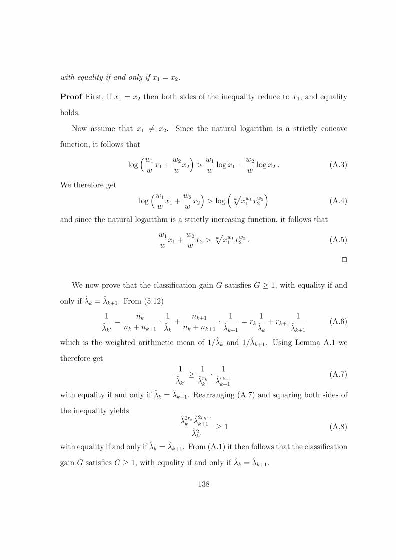
with equality if and only if x1 = x2.

Proof First, if x1 = x2 then both sides of the inequality reduce to x1, and equality

holds.

Now assume that x1 �= x2. Since the natural logarithm is a strictly concave

function, it follows that

log(w1

wx1 +

w2

wx2

)>

w1

wlog x1 +

w2

wlog x2 . (A.3)

We therefore get

log(w1

wx1 +

w2

wx2

)> log

(w√

xw11 xw2

2

)(A.4)

and since the natural logarithm is a strictly increasing function, it follows that

w1

wx1 +

w2

wx2 > w

√xw1

1 xw22 . (A.5)

�

We now prove that the classification gain G satisfies G ≥ 1, with equality if and

only if λk = λk+1. From (5.12)

1

λk′=

nk

nk + nk+1

· 1

λk

+nk+1

nk + nk+1

· 1

λk+1

= rk1

λk

+ rk+11

λk+1

(A.6)

which is the weighted arithmetic mean of 1/λk and 1/λk+1. Using Lemma A.1 we

therefore get

1

λk′≥ 1

λrkk

· 1

λrk+1

k+1

(A.7)

with equality if and only if λk = λk+1. Rearranging (A.7) and squaring both sides of

the inequality yields

λ2rkk λ

2rk+1

k+1

λ2k′

≥ 1 (A.8)

with equality if and only if λk = λk+1. From (A.1) it then follows that the classification

gain G satisfies G ≥ 1, with equality if and only if λk = λk+1.

138

Appendix B

Reconstruction Offsets of the

Optimal Uniform Threshold

Quantizer for the Laplacian

Distribution

An expression for the reconstruction levels of a uniform threshold quantizer (UTQ)

for the Laplacian distribution, optimized for minimum MSE distortion, was derived

in Section 6.1. In this appendix we prove that some of the reconstruction offsets of

this UTQ are equal.

Using the same notation as in Section 6.1, let λ (> 0) be the parameter of the

Laplacian distribution, let Δ be the step size of the UTQ, and denote the number of

levels of the UTQ by N = 2L + 1. The bin boundaries bj, j = 1, . . . , L, of the UTQ

are given in (6.5), and the bin probabilities pj, j = 1, . . . , L − 1, are given in (6.13).

139

From (6.14), we then get for the reconstruction levels qj, j = 1, . . . , L − 1 :

qj =1

2pj

[bje

−λbj − bj+1e−λbj+1

]+

1

λ=

=1

e−λbj − e−λbj+1

[(j − 1

2)Δe−λbj − (j − 1

2+ 1)Δe−λbj+1

]+

1

λ=

=1

e−λbj − e−λbj+1

[(j − 1

2)Δ

(e−λbj − e−λbj+1

)− Δe−λbj+1

]+

1

λ=

= (j − 1

2)Δ − Δ

e−λbj+1

e−λbj − e−λbj+1+

1

λ=

= (j − 1

2)Δ − Δ

e−λ(j+ 12)Δ

e−λ(j− 12)Δ − e−λ(j+ 1

2)Δ+

1

λ=

= (j − 1

2)Δ − Δ

e−λ(j− 12)Δ+λ(j+ 1

2)Δ − 1+

1

λ=

= (j − 1

2)Δ − Δ

eλΔ − 1+

1

λ=

= bj +1

λ− Δ

eλΔ − 1. (B.1)

Thus, the reconstruction offsets qj − bj, for j = 1, . . . , L − 1, do not depend on j.

Namely,

qj = bj + δ, j = 1, . . . , L − 1 , (B.2)

where

δ =1

λ− Δ

eλΔ − 1. (B.3)

140

Appendix C

Proof of a Useful Property of the

Laplacian Distribution

The following useful property of the Laplacian distribution is proved in this appendix.

Property C.1 Let X be a Laplacian random variable with parameter λ (> 0), i.e.,

fX(x) =λ

2e−λ|x|, −∞ < x < ∞ (C.1)

and let c be a fixed nonnegative real number. Then given that X ≥ c, the conditional

distribution of Y = X − c is exponential with parameter λ, i.e.,

fY |X≥c(y|X ≥ c) = λe−λy, y ≥ 0 . (C.2)

141

Proof The conditional density function of X, conditioned on X ≥ c, is given by

fX|X≥c(x|X ≥ c) =

⎧⎪⎨⎪⎩

fX(x)/∫∞

cfX(α) dα, x ≥ c

0, else=

=

⎧⎪⎨⎪⎩

λ2e−λx/

∫∞c

λ2e−λα dα, x ≥ c

0, else=

=

⎧⎪⎨⎪⎩

e−λx/(

1λe−λc

), x ≥ c

0, else=

=

⎧⎪⎨⎪⎩

λe−λ(x−c), x ≥ c

0, else. (C.3)

Defining Y = X − c, we get

fY |X≥c(y|X ≥ c) = λe−λy, y ≥ 0 . (C.4)

That is, given that X ≥ c, the conditional distribution of Y = X − c is exponential

with parameter λ. �

142

Appendix D

Squared Error Distortion of the

Optimal Uniform Threshold

Quantizer for the Laplacian

Distribution

An expression for the average squared error distortion of a uniform threshold quan-

tizer (UTQ) for the Laplacian distribution, optimized for minimum distortion, was

derived in Section 6.1. In this appendix we further develop this expression to obtain a

closed form expression for the average distortion D, whose evaluation does not involve

integration.

As in Section 6.1, let Δ be the step size of the UTQ. The bin boundaries {bj} of

the UTQ are given in (6.5), and the reconstruction levels {qj} are given in (6.12) and

143

(6.15). According to (6.17), the average distortion of the UTQ is then given by

D =

∫ b1

−b1

fX(x)(x − 0)2 dx + 2L−1∑j=1

∫ bj+1

bj

fX(x)(x − qj)2 dx + 2

∫ ∞

bL

fX(x)(x − qL)2 dx =

= 2

[∫ b1

0

x2fX(x) dx +L−1∑j=1

∫ bj+1

bj

(x − qj)2fX(x) dx +

∫ ∞

bL

(x − qL)2fX(x) dx

]=

= 2

[∫ b1

0

x2λ

2e−λx dx +

L−1∑j=1

∫ bj+1

bj

(x − qj)2 λ

2e−λx dx +

∫ ∞

bL

(x − qL)2λ

2e−λx dx

]=

= λ

[∫ b1

0

x2e−λx dx +L−1∑j=1

∫ bj+1

bj

(x − qj)2e−λx dx +

∫ ∞

bL

(x − qL)2e−λx dx

](D.1)

where λ (> 0) is the parameter of the Laplacian distribution, and the number of levels

of the quantizer is N = 2L + 1.

To calculate the above integrals, we use the following indefinite integral, obtained

directly using integration by parts:

∫x2e−λx dx = −1

λe−λx

(x2 +

2x

λ+

2

λ2

)+ C (D.2)

where C is an arbitrary constant of integration. The first term in the brackets of (D.1)

then becomes

∫ b1

0

x2e−λx dx =1

λ

[e−λx

(x2 +

2x

λ+

2

λ2

)]0

b1

=

=1

λ

[2

λ2− e−λb1

(b21 +

2b1

λ+

2

λ2

)]=

=1

λ

[2

λ2− e−λΔ

2

((Δ

2

)2

+Δ

λ+

2

λ2

)]. (D.3)

The second term in the brackets of (D.1) is calculated in a similar manner, along with

the substitution of variables t = x − qj (translation), as follows. From (6.15) we get

qj − bj = δ, j = 1, . . . , L − 1 , (D.4)

144

where

δ =1

λ− Δ

eλΔ − 1. (D.5)

We thus obtain for the second term

L−1∑j=1

∫ bj+1

bj

(x − qj)2e−λx dx =

L−1∑j=1

∫ bj+1−qj

bj−qj

t2e−λ(t+qj) dt =

=L−1∑j=1

e−λqj

∫ −δ+Δ

−δ

t2e−λt dt =

=L−1∑j=1

e−λqj1

λ

[e−λt

(t2 +

2t

λ+

2

λ2

)]−δ

−δ+Δ

=

=1

λ

(L−1∑j=1

e−λqj

)·[eλδ

(δ2 − 2δ

λ+

2

λ2

)+

− eλ(δ−Δ)

((δ − Δ)2 − 2(δ − Δ)

λ+

2

λ2

)].(D.6)

Similarly, for the third term in the brackets of (D.1), using (6.12) and the substitution

of variables t = x − qL, we get

∫ ∞

bL

(x − qL)2e−λx dx =

∫ ∞

bL−qL

t2e−λ(t+qL) dt = e−λqL

∫ ∞

− 1λ

t2e−λt dt =

= e−λqL1

λ

[e−λt

(t2 +

2t

λ+

2

λ2

)]− 1λ

∞=

=1

λe−λqL · e ·

(1

λ2− 2

λ2+

2

λ2

)=

=1

λ3e1−λqL . (D.7)

From (D.1), (D.3), (D.6) and (D.7), we finally obtain a closed form expression for

145

the average distortion of the UTQ:

D =2

λ2− e−λΔ

2

((Δ

2

)2

+Δ

λ+

2

λ2

)+

+

(L−1∑j=1

e−λqj

)·[eλδ

(δ2 − 2δ

λ+

2

λ2

)− eλ(δ−Δ)

((δ − Δ)2 − 2(δ − Δ)

λ+

2

λ2

)]+

+1

λ2e1−λqL (D.8)

where δ is given in (D.5), and where

qj = bj + δ = (j − 1

2)Δ + δ, j = 1, . . . , L − 1 (D.9)

and

qL = bL +1

λ= (L − 1

2)Δ +

1

λ. (D.10)

146

Appendix E

Squared Error Distortion of the

Uniform Reconstruction with

Unity Ratio Quantizer for the

Laplacian Distribution

The uniform reconstruction with unity ratio quantizer (URURQ) for the Laplacian

distribution was presented in Section 6.2. In this appendix we derive a closed form

expression for the average squared error distortion D of the URURQ, whose evaluation

does not involve integration.

Using the same notation as in Section 6.2, let λ (> 0) be the parameter of the

Laplacian distribution, let Δ be the step size of the URURQ, and denote the number

of levels of the URURQ by N = 2L+1. Following Appendix D, the average distortion

147

of the URURQ is given by

D = λ

[∫ b1

0

x2e−λx dx +L−1∑j=1

∫ bj+1

bj

(x − qj)2e−λx dx +

∫ ∞

bL

(x − qL)2e−λx dx

](E.1)

where the bin boundaries {bj} and the reconstruction levels {qj} of the URURQ are

defined in Section 6.2. Note that since the number of levels is finite, we optimize

the outermost reconstruction levels (i.e., qL and q−L) for minimum MSE distortion,

according to the well-known centroid condition. This yields

qL = E [X|X > bL] = bL + E [X − bL|X > bL] = bL +1

λ(E.2)

where the last equality follows from the fact that given that X > bL, the conditional

distribution of X − bL is exponential with parameter λ (see Appendix C), and thus

has a mean of 1/λ.

Using the indefinite integral (D.2), the first term in the brackets of (E.1) is given

by ∫ b1

0

x2e−λx dx =1

λ

[e−λx

(x2 +

2x

λ+

2

λ2

)]0

b1

=

=1

λ

[2

λ2− e−λb1

(b21 +

2b1

λ+

2

λ2

)]=

=1

λ

[2

λ2− eλ(δ−Δ)

((δ − Δ)2 − 2(δ − Δ)

λ+

2

λ2

)](E.3)

where

δ = δ(Δ) =1

λ− Δ

eλΔ − 1. (E.4)

Since qj − bj = δ , for j = 1, . . . , L − 1 , we obtain, following Appendix D, for the

second and the third terms in the brackets of (E.1)

L−1∑j=1

∫ bj+1

bj

(x − qj)2e−λx dx =

1

λ

(L−1∑j=1

e−λqj

)·[eλδ

(δ2 − 2δ

λ+

2

λ2

)+

− eλ(δ−Δ)

((δ − Δ)2 − 2(δ − Δ)

λ+

2

λ2

)],(E.5)

148

and ∫ ∞

bL

(x − qL)2e−λx dx =1

λ3e1−λqL , (E.6)

respectively.

From (E.1), (E.3), (E.5) and (E.6), we finally obtain a closed form expression for

the average distortion of the URURQ:

D =2

λ2− eλ(δ−Δ)

((δ − Δ)2 − 2(δ − Δ)

λ+

2

λ2

)+

+

(L−1∑j=1

e−λqj

)·[eλδ

(δ2 − 2δ

λ+

2

λ2

)− eλ(δ−Δ)

((δ − Δ)2 − 2(δ − Δ)

λ+

2

λ2

)]+

+1

λ2e1−λqL (E.7)

where δ is given in (E.4), and where

qj = jΔ , j = 1, . . . , L − 1 (E.8)

and

qL = bL +1

λ= LΔ − δ +

1

λ. (E.9)

149

References

[1] M. Antonini, M. Barlaud, P. Mathieu, and I. Daubechies, “Image coding

using wavelet transform,” IEEE Trans. Image Process., vol. 1, no. 2, pp.

205–220, Apr 1992.

[2] S. Arimoto, “An algorithm for computing the capacity of arbitrary discrete

memoryless channels,” IEEE Trans. Inf. Theory, vol. 18, no. 1, pp. 14–20,

Jan 1972.

[3] J.-C. Batllo and V. A. Vaishampayan, “Asymptotic performance of multi-

ple description transform codes,” IEEE Trans. Inf. Theory, vol. 43, no. 2,

pp. 703–707, Mar 1997.

[4] T. Berger, Rate Distortion Theory: A Mathematical Basis for Data Com-

pression. Englewood Cliffs, NJ: Prentice-Hall, 1971.

[5] ——, “Minimum entropy quantizers and permutation codes,” IEEE Trans.

Inf. Theory, vol. 28, no. 2, pp. 149–157, Mar 1982.

[6] K. A. Birney and T. R. Fischer, “On the modeling of DCT and subband

image data for compression,” IEEE Trans. Image Process., vol. 4, no. 2,

pp. 186–193, Feb 1995.

150

[7] R. Blahut, “Computation of channel capacity and rate-distortion func-

tions,” IEEE Trans. Inf. Theory, vol. 18, no. 4, pp. 460–473, Jul 1972.

[8] J. N. Bradley and C. M. Brislawn, “The wavelet/scalar quantization com-

pression standard for digital fingerprint images,” in Proc. IEEE Int. Sym-

posium on Circuits and Systems, May–Jun 1994, vol. 3, pp. 205–208.

[9] R. W. Buccigrossi and E. P. Simoncelli, “Image compression via joint statis-

tical characterization in the wavelet domain,” IEEE Trans. Image Process.,

vol. 8, no. 12, pp. 1688–1701, Dec 1999.

[10] T. Chiang and Y.-Q. Zhang, “A new rate control scheme using quadratic

rate distortion model,” IEEE Trans. Circuits Syst. Video Technol., vol. 7,

no. 1, pp. 246–250, Feb 1997.

[11] A. Cohen, I. Daubechies, and J.-C. Feauveau, “Biorthogonal bases of com-

pactly supported wavelets,” Commun. Pure and Appl. Math., vol. 45, pp.

485–560, 1992.

[12] J. H. Conway and N. J. A. Sloane, “Fast quantizing and decoding algo-

rithms for lattice quantizers and codes,” IEEE Trans. Inf. Theory, vol. 28,

no. 2, pp. 227–232, Mar 1982.

[13] T. M. Cover and J. A. Thomas, Elements of Information Theory. New

York: Wiley, 1991.

[14] I. Daubechies, “Orthonormal bases of compactly supported wavelets,”

Commun. Pure and Appl. Math., vol. XLI, pp. 909–996, 1988.

151

[15] A. A. El Gamal and T. M. Cover, “Achievable rates for multiple descrip-

tions,” IEEE Trans. Inf. Theory, vol. 28, no. 6, pp. 851–857, Nov 1982.

[16] N. Farvardin and J. Modestino, “Optimum quantizer performance for

a class of non-Gaussian memoryless sources,” IEEE Trans. Inf. Theory,

vol. 30, no. 3, pp. 485–497, May 1984.

[17] M. Fleming and M. Effros, “Generalized multiple description vector quanti-

zation,” in Proc. IEEE Data Compression Conf., Snowbird, UT, Mar 1999,

pp. 3–12.

[18] Y. Frank-Dayan and R. Zamir, “Universal lattice-based quantizers for mul-

tiple descriptions,” in Proc. IEEE Data Compression Conf., Snowbird, UT,

Mar 2000, pp. 500–509.

[19] R. C. Gonzalez and R. E. Woods, Digital Image Processing, 3rd ed. Pren-

tice Hall, 2008.

[20] V. K. Goyal, “Single and multiple description transform coding with bases

and frames,” Philadelphia, PA: SIAM, 2001.

[21] ——, “Multiple description coding: compression meets the network,” IEEE

Signal Process. Mag., vol. 18, no. 5, pp. 74–93, Sep 2001.

[22] ——, “Theoretical foundations of transform coding,” IEEE Signal Process.

Mag., vol. 18, no. 5, pp. 9–21, Sep 2001.

[23] V. K. Goyal and J. Kovacevic, “Optimal multiple description transform

coding of Gaussian vectors,” in Proc. IEEE Data Compression Conf.,

Snowbird, UT, Mar–Apr 1998, pp. 388–397.

152

[24] ——, “Generalized multiple description coding with correlating trans-

forms,” IEEE Trans. Inf. Theory, vol. 47, no. 6, pp. 2199–2224, Sep 2001.

[25] R. M. Gray and D. L. Neuhoff, “Quantization,” IEEE Trans. Inf. Theory,

vol. 44, no. 6, pp. 2325–2383, Oct 1998.

[26] H. Jafarkhani and V. Tarokh, “Multiple description trellis-coded quantiza-

tion,” IEEE Trans. Commun., vol. 47, no. 6, pp. 799–803, Jun 1999.

[27] A. K. Jain, Fundamentals of Digital Image Processing. Englewood Cliffs,

NJ: Prentice-Hall, 1989.

[28] N. S. Janyant, “Subsampling of a DPCM speech channel to provide two

‘self-contained’ half-rate channels,” Bell Syst. Tech. J., vol. 60, no. 4, pp.

501–509, Apr 1981.

[29] N. S. Jayant and S. W. Christensen, “Effects of packet losses in waveform

coded speech and improvements due to an odd-even sample-interpolation

procedure,” IEEE Trans. Commun., vol. 29, no. 2, pp. 101–109, Feb 1981.

[30] W. Jiang and A. Ortega, “Multiple description coding via polyphase trans-

form and selective quantization,” in Proc. Visual Communic. and Image

Proc., San Jose, CA, Jan 1999, pp. 998–1008.

[31] R. L. Joshi, V. J. Crump, and T. R. Fischer, “Image subband coding using

arithmetic coded trellis coded quantization,” IEEE Trans. Circuits Syst.

Video Technol., vol. 5, no. 6, pp. 515–523, Dec 1995.

153

[32] R. L. Joshi, T. R. Fischer, and R. H. Bamberger, “Optimum classification

in subband coding of images,” in Proc. IEEE Int. Conf. Image Processing,

Austin, Texas, Nov 1994, vol. 2, pp. 883–887.

[33] R. L. Joshi, H. Jafarkhani, J. H. Kasner, T. R. Fischer, N. Farvardin,

M. W. Marcellin, and R. H. Bamberger, “Comparison of different methods

of classification in subband coding of images,” IEEE Trans. Image Process.,

vol. 6, no. 11, pp. 1473–1486, Nov 1997.

[34] S. M. Kay, Fundamentals of Statistical Signal Processing: Estimation The-

ory. Englewood Cliffs, NJ: Prentice-Hall, 1993.

[35] M. Lightstone, E. Majani, and S. K. Mitra, “Low bit-rate design consid-

erations for wavelet-based image coding,” Multidimensional Syst. Signal

Processing, vol. 8, pp. 111–128, Jan 1997.

[36] S. M. LoPresto, K. Ramchandran, and M. T. Orchard, “Image coding

based on mixture modeling of wavelet coefficients and a fast estimation-

quantization framework,” in Proc. Data Compression Conf., Mar 1997, pp.

221–230.

[37] S. G. Mallat, “A theory for multiresolution signal decomposition: the

wavelet representation,” IEEE Trans. Pattern Anal. Mach. Intell., vol. 11,

no. 7, pp. 674–693, Jul 1989.

[38] A. E. Mohr, E. A. Riskin, and R. E. Ladner, “Unequal loss protection:

graceful degradation of image quality over packet erasure channels through

forward error correction,” IEEE J. Select. Areas Commun., vol. 18, no. 6,

pp. 819–828, Jun 2000.

154

[39] M. T. Orchard, Y. Wang, V. A. Vaishampayan, and A. R. Reibman, “Re-

dundancy rate-distortion analysis of multiple description coding using pair-

wise correlating transforms,” in Proc. IEEE Int. Conf. Image Processing,

Santa Barbara, CA, Oct 1997, vol. 1, pp. 608–611.

[40] A. Ortega and K. Ramchandran, “Rate-distortion methods for image and

video compression,” IEEE Signal Process. Mag., vol. 15, no. 6, pp. 23–50,

Nov 1998.

[41] L. Ozarow, “On a source-coding problem with two channels and three

receivers,” Bell Syst. Tech. J., vol. 59, no. 10, pp. 1909–1921, Dec 1980.

[42] W. H. Press, S. A. Teukolsky, W. T. Vetterling, and B. P. Flannery, Nu-

merical Recipes: The Art of Scientific Computing, 3rd ed. Cambridge

University Press, 2007.

[43] R. Puri and K. Ramchandran, “Multiple description source coding using

forward error correction codes,” in Conf. Rec. 33rd Asilomar Conf. Sig.,

Sys. & Computers, Pacific Grove, CA, Oct 1999, vol. 1, pp. 342–346.

[44] D. O. Reudink, “The channel splitting problem with interpolative coders,”

Bell Labs, Tech. Rep. TM80-134-1, Oct 1980.

[45] A. Said and W. A. Pearlman, “A new, fast, and efficient image codec based

on set partitioning in hierarchical trees,” IEEE Trans. Circuits Syst. Video

Technol., vol. 6, no. 3, pp. 243–250, Jun 1996.

[46] S. D. Servetto, K. Ramchandran, V. A. Vaishampayan, and K. Nahrstedt,

“Multiple-description wavelet based image coding,” in Proc. IEEE Int.

Conf. Image Processing, Oct 1998, vol. 1, pp. 659–663.

155

[47] S. D. Servetto, V. A. Vaishampayan, and N. J. A. Sloane, “Multiple de-

scription lattice vector quantization,” in Proc. IEEE Data Compression

Conf., Snowbird, UT, Mar 1999, pp. 13–22.

[48] C. E. Shannon, “Coding theorems for a discrete source with a fidelity

criterion,” IRE Nat. Conv. Rec., Mar 1959, reprinted in Key Papers in the

Development of Information Theory. New York: IEEE.

[49] J. M. Shapiro, “Embedded image coding using zerotrees of wavelet coeffi-

cients,” IEEE Trans. Signal Process., vol. 41, no. 12, pp. 3445–3462, Dec

1993.

[50] Y. Shoham and A. Gersho, “Efficient bit allocation for an arbitrary set of

quantizers,” IEEE Trans. Acoust., Speech, Signal Process., vol. 36, no. 9,

pp. 1445–1453, Sep 1988.

[51] G. Strang and T. Nguyen, Wavelets and Filter Banks, 2nd ed. Wellesley-

Cambridge Press, 1996.

[52] P. Subrahmanya and T. Berger, “Multiple descriptions encoding of im-

ages,” in Proc. IEEE Data Compression Conf., Snowbird, UT, Mar 1997,

p. 470.

[53] G. J. Sullivan, “Efficient scalar quantization of exponential and Laplacian

random variables,” IEEE Trans. Inf. Theory, vol. 42, no. 5, pp. 1365–1374,

Sep 1996.

[54] N. Tanabe and N. Farvardin, “Subband image coding using entropy-coded

quantization over noisy channels,” IEEE J. Sel. Areas Commun., vol. 10,

no. 5, pp. 926–943, Jun 1992.

156

[55] D. S. Taubman and M. W. Marcellin, JPEG2000: Image Compression

Fundamentals, Standards and Practice. Springer, 2002.

[56] B. E. Usevitch, “Optimal bit allocation for biorthogonal wavelet coding,”

in Proc. IEEE Data Compression Conf., Snowbird, UT, Mar–Apr 1996,

pp. 387–395.

[57] ——, “A tutorial on modern lossy wavelet image compression: foundations

of JPEG 2000,” IEEE Signal Process. Mag., vol. 18, no. 5, pp. 22–35, Sep

2001.

[58] B. E. Usevitch and M. T. Orchard, “Smooth wavelets, transform coding,

and Markov-1 processes,” IEEE Trans. Signal Process., vol. 43, no. 11, pp.

2561–2569, Nov 1995.

[59] V. A. Vaishampayan, “Design of multiple description scalar quantizers,”

IEEE Trans. Inf. Theory, vol. 39, no. 3, pp. 821–834, May 1993.

[60] V. A. Vaishampayan and J.-C. Batllo, “Asymptotic analysis of multiple

description quantizers,” IEEE Trans. Inf. Theory, vol. 44, no. 1, pp. 278–

284, Jan 1998.

[61] V. A. Vaishampayan and J. Domaszewicz, “Design of entropy-constrained

multiple-description scalar quantizers,” IEEE Trans. Inf. Theory, vol. 40,

no. 1, pp. 245–250, Jan 1994.

[62] V. A. Vaishampayan, N. J. A. Sloane, and S. D. Servetto, “Multiple-

description vector quantization with lattice codebooks: design and analy-

sis,” IEEE Trans. Inf. Theory, vol. 47, no. 5, pp. 1718–1734, Jul 2001.

157

[63] R. Venkataramani, G. Kramer, and V. K. Goyal, “Multiple description

coding with many channels,” IEEE Trans. Inf. Theory, vol. 49, no. 9, pp.

2106–2114, Sep 2003.

[64] J. D. Villasenor, B. Belzer, and J. Liao, “Wavelet filter evaluation for image

compression,” IEEE Trans. Image Process., vol. 4, no. 8, pp. 1053–1060,

Aug 1995.

[65] Y. Wang, M. T. Orchard, and A. R. Reibman, “Multiple description image

coding for noisy channels by pairing transform coefficients,” in Proc. IEEE

Workshop on Multimedia Signal Processing, Princeton, NJ, Jun 1997, pp.

419–424.

[66] Y. Yoo, A. Ortega, and B. Yu, “Image subband coding using context-

based classification and adaptive quantization,” IEEE Trans. Image Pro-

cess., vol. 8, no. 12, pp. 1702–1715, Dec 1999.

[67] R. Zamir, “Gaussian codes and shannon bounds for multiple descriptions,”

IEEE Trans. Inf. Theory, vol. 45, no. 7, pp. 2629–2636, Nov 1999.

[68] Z. Zhang and T. Berger, “New results in binary multiple descriptions,”

IEEE Trans. Inf. Theory, vol. 33, no. 4, pp. 502–521, Jul 1987.

��

��

Wavelet� ��

��

��

Wavelet� ��

��

��

� ��

��

�� — ��

��

��

��

��

��

��

� ��

�� SIPL�

��

��

��

��

� ��

� ��

� ��

� ��

� � � � � � � � � � � � � � � � � � � � � � � � � � � � � � � ��

��

� � � � � � � � � � � � � � � � � � � � � � � � � � � � � � � � � � � � ��

��

� � � � � � � � � � � � � � � � � � � � � � � � � ��

� � � � � � � � � � � � � � � � � � � � � � � � � � � ��

��

��

��

��

��

�

��

� � � � � � � � � � � � � � � � � � � � � � � � � � � � � � � � � � ��

�Wavelet��

��

� � � � � � � � � � � � � � � � � � � � � � � � � � � � � � � � � � � � � � � ��

� � � � � � � � � � � � � � � � � � � � � � � � � � �� Wavelet ��

�� Wavelet ��

��

�Wavelet��

��

� � � � � � � � � � � � � � � � � � � � � � � � � � � � � � � � � � � � � � � � ��

� � � � � � � � � � � � � � � � � � � � � � � � � � � � � � � � � � � � � � !��

�� !�� "��

�Wavelet��

��

�� UTQ !�� #��

� � � � � � � � UTQ !�� $��#�� %� URURQ !�� $��#��

� � � � � � � � � � � � � � � � � � � ��

�Wavelet��

��

� � � � � � � � � � � � � � � � � � � � � � � � � � � � � � � � � � � � ��

� � � � � � � � � � � � � � � � � � Wavelet �� ! ��%� ��

�� !�� Wavelet ��

�

��

��

��

��

��

��

��

� � � � � � � � !�� "�� #

��

�� "��

��

�� $� ��

�� G ≥ 1 �� Classification Gain��

�� UTQ ��

��

�� UTQ �� !

�� URURQ ��

��

� ��

��

��

�� 2M − 1�� M ��

�� ρ ��

�� r ��

��

�� !� ��

�" � � � � � � � � � � � � � � � � � � � � � � ��

��

# � � � � � � � � � � � � � � � � � � � � � � � � � � � � � � � � � � � � � ��

��

� � � � � � � � � � � � � � � � � � � � � � � � � ��

�� $Lena ��

�� 1 bpp �

� � � � � � � � �MDSQ � ��

% � � � � � � � � � � � � � �� K �� Wavelet ��

�


��

��



�� s = 1.5 � r = 1 ��

�� ! �� "

�" � � � � � � � � � � � � � � � � � � � � � � � � � � � � � � � � � � �C #�� Wavelet

�� $�� %

�� $� ��

"� � � � � � � � � � � � � �� MD�� &

"� � � � � � � � � � � � � �� MD��

"% � � � � � � � � � � � � � � � � � � � � �Xi,j #�� Wavelet ��

"� � � � � � � � � � � �Ai,j �� Activity�� Xi,j ��

%� � � � � � � �� $��

%� � �N = 2L + 1 ��$�� Δ �� UTQ � �$�� "��

UTQ � �� $�� "��

&� � � � � � � ��

&� �N = 2L + 1 ��$�� Δ �� URURQ � �$�� "��

�� ! �Whole-point � Half-point � �� %��

�" � � � � � � � �Whole-point � �� ! �Half-point � ��

�'� � � � � � �� Xi,j �� $�� %��

�� (�$��(� �� ! �� %��

�'� � � � � � � � � � � � � � � � � � � � � � � � � � � � �Xi−1,j−1 ��

$

�� Plain polyphase transform� ��

�� MD��

�� 512 × 512 ��

�� Goldhill �� Lena ��

�� Lena �� Wavelet �� !

��

��

��! � � � � � � �� "�� #

��# � � � � � � � � � � � � � � � �Lena �� MD�� $

��$ � � � � � � � � � � � � � �Goldhill �� MD�� %

�� MD�� &

��& � � � � � � � � � � � � � � � � � � � � � � � � � � � ��

�� MD��

��' � � � � � � � � � � � � � � � � � � � � � � � � � � � ��Goldhill �� SD

�� MD�� '

�� Lena �� SD

�� MD��

�� Subband "� "�

�URURQ �� MD��

��! � � � � � � � � � � � � � � � � � �UTQ ��

�� “No-context coder”��

��$ � � � � � � � � � � � � � � � � � � � � ��

�� "�� " �� MD�� !

�� "��

�

��

��

�

��

�� Index assignment��



�� Wavelet �� Energy gain factors� ��

�� CDF 9/7 ��

��

�� Multiple description—MD� ��

��

��

��

��

��

�� Layered coding� ��

��

��

��

��

��

��

��

��

��

�� Wavelet

�� MD scalar quantization—MDSQ� ��

��

�� MD correlating transforms� ��

��

��

��

��

��

��

�� Wavelet��

��

��

��

��

��

��


��

��

��

�� MD��

��

�� Wavelet

��


��

��

�

��

��

��

��

��

��

��

��

�� Uniform threshold quantizer� UTQ ��

�� Uniform reconstruction with unity ratio quantizer� URURQ ��

Entropy-constrained� ��!��

�� scalar quantizer—ECSQ

� ��

�� !��

�� Off-line� �� Indexed� ��

��

�� UTQ� ��

�URURQ� ��

�� Subbands� ��

��

�� Wavelet� �� "��

Variance� ��

�� scaling

�� On-line� � � ��

��

��

��

�� MD��

��

��

��


�� MD��

��

��

webee.technion.ac.ilwebee.technion.ac.il/Sites/People/DavidMalah/Pubs/FP/Dror-Porat... · THIS...

Documents

Transcript of webee.technion.ac.ilwebee.technion.ac.il/Sites/People/DavidMalah/Pubs/FP/Dror-Porat... · THIS...