Web viewGeometry-related functions. Much like available commercial softwares, ... operations (such...

[100] 011 Chapter 11 Matrix, Tutorial by www.msharpmath.com

[100] 011 revised on 2012.12.03 cemmath

The Simple is the Best

Chapter 11 Matrix

11-1 Creating Matrices11-2 Subscripts for elements11-3 Operations for Matrices11-4 Relational and Conditional Operations11-5 Special Binary Operations11-6 Rows, Columns and Diagonals11-7 Submatrices11-8 ‘figure’ Related Functions11-9 ‘matrix’-Returning Functions11-10 ‘poly’ and ‘double’ Related Functions11-11 Several Useful Member Functions11-12 Matrix Functions and Array of Matrices11-13 Special Matrices11-14 Application to Triangle Solution11-15 Summary ■ Creating matrices ■ Subscripts ■ Read and Write ■ Unary Operations ■ Binary Operations ■ Conditional Operations ■ Relational Operations ■ Submatrices ■ Deleting Elements ■ figure-Returning Functions ■ poly-Returning Functions ■ double-Returning Functions ■ matrix-Returning Functions ■ Tuple-Returning Functions

1

http://www.msharpmath.com/


■ Tensor-Related Functions ■ Matrix Declaration ■ Geometry-related functions

Much like available commercial softwares, Cemmath adopts class ‘matrix’ as the most valuable data structure. For concise explanation, we employ mathematical expressions

A=(aij )=[ a11 a12 … a1n

a21 a22 ⋯ a2n

⋮ ⋮ ⋱ ⋮am1 am2 ⋯ amn

]Most operations on matrices will be explained by representative elements, for example ( aij ). We presume that readers are familiar with matrix operations from mathematics.

Section 11-1 Creating Matrices

■ List of numbers. A simple way of creating a matrix is placing numbers inside a pair of brackets

// list of numbers or matrices inside [] [ a11, ... , a1n ; a21, ... , a2n ; ... a_mn ]

for example

%> separate rows by ';' and elements by ','#> A = [ 1, 2, 3 ; 4, 5 ; 6 ];A = [ 1 2 3 ] [ 4 5 0 ] [ 6 0 0 ]

Each element is listed row-wise, and each row is separated by a semicolon. Any matrix can be placed inside a pair of [] to make a matrix

2



#> [ A, -A ; 2*A ];ans = [ 1 2 3 -1 -2 -3 ] [ 4 5 0 -4 -5 -0 ] [ 6 0 0 -6 -0 -0 ] [ 2 4 6 0 0 0 ] [ 8 10 0 0 0 0 ] [ 12 0 0 0 0 0 ]

In particular, a null matrix of dimension 0× 0 is denoted by a pair of []

#> [] ; // 0 x 0 matrix ans = []

Another easy way of creating matrices is using a colon ':'

a : b // [ a, a+1, ... ] if a < b, otherwise [ a, a-1, ... ] a : h : b // [ a, a+h, a+2h, ... ], the same as (a,b).step(h)

#> 1 : 5 ; ans = [ 1 2 3 4 5 ]

#> 5 : 1 ; ans = [ 5 4 3 2 1 ]

#> 1 : 0.2 : 2 ; ans = [ 1 1.2 1.4 1.6 1.8 2 ]

■ Tuple functions. An interval (a,b) is a geometrical concept, while grid number and ratio are numerical concepts. These are separated by tuple functions

(a,b) .step(h) // the same as a : h : b(a,b) .span(n,g=1) // [ x_1 = a, x_2, ..., x_n = b ], dx_i = g*dx_(i-1)(a,h) .march(n,g=1) // [ a, a+h(1), a+h(1+g), ... , a+h(1+...+g^(n-2)) ](a,b) .logspan(n,g=1) // equal to 10.^( (log10(a),log10(b)).span(n,g=1) )

The first one is the same as (a:h:b) and thus is skipped. To implement geometrically varying grid size, we use two methods. One works inside an interval (a,b), and the other works toward a direction.

#> (0,15) .span(6); // g=1 (by default) for uniform span

3



ans = [ 0 3 6 9 12 15 ]

#> X = (0,15).span(5,2); // g=2 for increasing, dX = [ 1,2,4,8 ] X = [ 0 1 3 7 15 ]

#> X = (0,15).span(5,0.5); // g=0.5 for decreasing dX = [ 8,4,2,1 ] X = [ 0 8 12 14 15 ]

// g=-2 for symmetric increasing, dX = [ 1,2,4,4,2,1 ]#> X = (1,15).span(7,-2); X = [ 1 2 4 8 12 14 15 ]

// g=-0.5 for symmetric decreasing, dX = [ 4,2,1,2,4 ]#> X = (1,14).span(6,-0.5); X = [ 1 5 7 8 10 14 ]

A geometrical marching is fulfilled by (a,b).march(n,g=1)

#> X = (3,1).march(6); // g=1 by default X = [ 3 4 5 6 7 8 ]

#> X = (3,1).march(6,2); // g=2 for increasing X = [ 3 4 6 10 18 34 ]

#> X = (3,1).march(6,0.5); // g=0.5 for decreasing X = [ 3 4 4.5 4.75 4.875 4.9375 ]

A tuple function (a,b).logspan(n,g=1) is used as follows.

#> x = (1,10).logspan(11); log10(x); x = [ 1 1.2589 1.5849 1.9953 2.5119 3.1623 3.9811

5.0119 6.3096 7.9433 10 ] ans = [ 0 0.1 0.2 0.3 0.4 0.5 0.6

0.7 0.8 0.9 1 ]

■ Well-known matrices. Matrices with all-zeros or all-ones as well as unity matrices are of fundamental importance. They can be created by dot functions

.e_k(n) // k-th unit vector in the n-dimensional space.I(m,n=m) eye(m,n=m) // a ij=0 (i ≠ j ) , aij=1(i= j)ones(m,n=m) // a ij=1

4



zeros(m,n=m) // a ij=0

which result in n ×1 or m× n matrices. The default option ‘n=m’ means that

// .ones(m) is equivalent to .ones(m,m)

When a matrix ‘A’ of dimension m× n already exists, it is possible to use the existing matrix ‘A’ as an argument to deliver the matrix dimension. In other words,

.I(A) eye(A) ones(A) zeros(A)

are all valid commands.

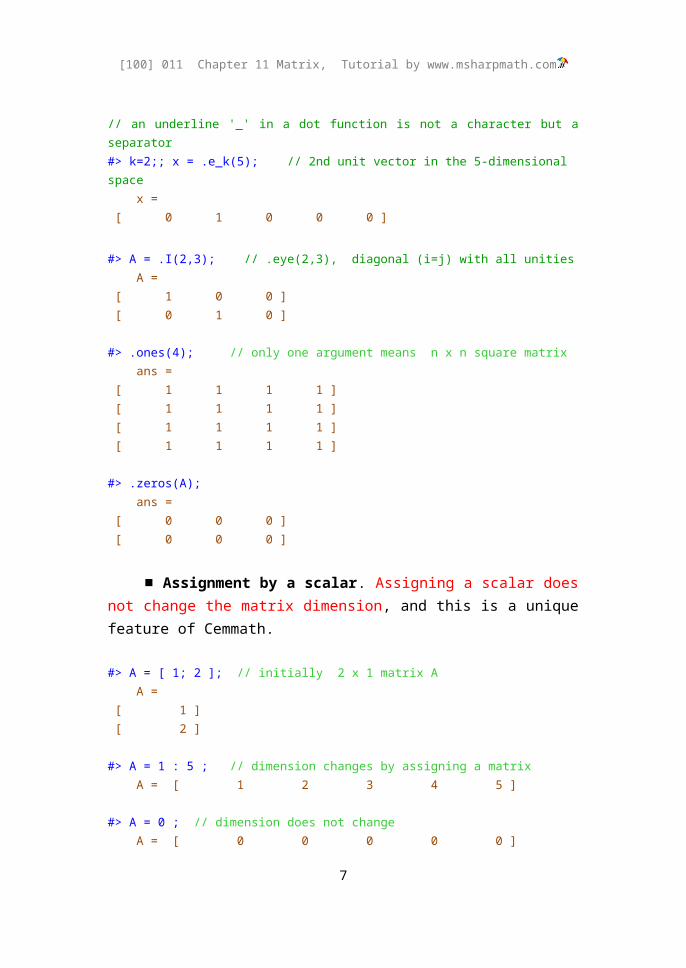
// an underline '_' in a dot function is not a character but a separator#> k=2;; x = .e_k(5); // 2nd unit vector in the 5-dimensional space x = [ 0 1 0 0 0 ]

#> A = .I(2,3); // .eye(2,3), diagonal (i=j) with all unities A = [ 1 0 0 ] [ 0 1 0 ]

#> .ones(4); // only one argument means n x n square matrix ans = [ 1 1 1 1 ] [ 1 1 1 1 ] [ 1 1 1 1 ] [ 1 1 1 1 ]

#> .zeros(A); ans = [ 0 0 0 ] [ 0 0 0 ]

■ Assignment by a scalar. Assigning a scalar does not change the matrix dimension, and this is a unique feature of Cemmath.

5



#> A = [ 1; 2 ]; // initially 2 x 1 matrix A A = [ 1 ] [ 2 ]

#> A = 1 : 5 ; // dimension changes by assigning a matrix A = [ 1 2 3 4 5 ]

#> A = 0 ; // dimension does not change A = [ 0 0 0 0 0 ]

■ Displaying matrices. In displaying matrices, delimiters (i.e. a pair of brackets) for each row and the number format for matrix can be changed, for example, by

#> matrix.format("%15.4e"); // default is matrix.format("") #> matrix.left(""); // left row-delimiter blank#> matrix.right(""); // right row-delimiter blank#> A = [ 1, 2, 3 ; 4, 5, 6 ];

Then, blanks replace both ‘[’ and ‘]’, and the number format is also changed

A = 1.0000e+000 2.0000e+000 3.0000e+000 4.0000e+000 5.0000e+000 6.0000e+000

The default format is imposed by a null string "" which is equivalent to "%15.6g". In other words,

#> matrix.format(""); // equivalent to matrix.format("%15.6g");

returns to the default format. The maximum column length displayed on the screen is set by default to be 10, and can be changed by

matrix.maxcol(n=10);

■ Reading/Writing Matrices. A matrix can be read from a file or written to a file by ‘read(string)’ and ‘write(string)’.

%> read/write matrix#> A = [1,2,3;4,5,6];; A.write("A_mtrx");#> B = [ 0,1 ]; B.read("A_mtrx"); B;

6



B = [ 0 1 ]B =[ 1 2 3 ][ 4 5 6 ]

Section 11-2 Subscripts for elements

■ Reference to Element. For a complex matrix A=X+iY , two-dimensional indexing of the element a ij

is carried out in three different ways

A(i,j) // real element only =x ij, works for read and writeA{i,j} // imaginary element only =y ij, works for read and write

A[i,j] // complex element =x ij+i y ij, works for read and write

Therefore, both ‘A(i,j)’ and ‘A{i,j}’ are treated as ‘double’, whereas ‘A[i,j]’ is treated as ‘complex’. The distinction between the real, imaginary and complex parts of a matrix is unique in Cemmath. The reason for this is that Cemmath strives to be compatible with the C-language, and thus the data type must be, at least implicitly, declared to handle variable data types. Mathematically, it can be seen that

A[i,j] = A(i,j) + i A{i,j}

Reading and writing are carried out for the elements. A simple example is as follows.

#> A = [ 7, 8 ];A = [ 7 8 ]

#> A[1,2] = 3-4!; A[1,2]; A; // writing and reading complex elementans = 3 - 4!ans = 3 - 4!A = [ 7 3 - i 4 ]

#> A(1,2) = 100; A(1,2); A; // writing and reading real partans = 100ans = 100

7



A = [ 7 100 - i 4 ]

#> A{1,2} = 200; A{1,2}; A; // writing and reading imaginary partans = 200ans = 200A = [ 7 100 + i 200 ]

■ A Special Index. In addition, a special index ‘end’ can be utilized to designate an element in the last row/column. An example is

#> A = [ 1-1!, 3-3!; 2-2!, 4-4! ];A = [ 1 - i 1 3 - i 3 ] [ 2 - i 2 4 - i 4 ]

#> A(end-1,end-1) = 100;; A;A = [ 100 - i 1 3 - i 3 ] [ 2 - i 2 4 - i 4 ]

#> A{end,end-1} *= 100;; A;A = [ 100 - i 1 3 - i 3 ] [ 2 - i 200 4 - i 4 ]

#> A[end,end] = 300-300!;; A;A = [ 100 - i 1 3 - i 3 ] [ 2 - i 200 300 - i 300 ]

■ One-Dimensional Treatment. For an m× n matrix A, it is also possible to treat the matrix elements as a one-dimensional array, for example

A=(ak)=[a1 a1+m … a1+m (n−1 )

a2 a2+m ⋯ a2+m (n−1 )

⋮ ⋮ ⋱ ⋮am a2m ⋯ amn

] , k=i+m( j−1)

In this regard, a one-dimensional indexing is also provided

8



A( k ) // real part only = xk

A{ k } // imaginary part only = yk

A[ k ] // complex element = xk+i yk

where both ‘A(k)’ and ‘A{k}’ are treated as ‘double’, whereas ‘A[k]’ is treated as ‘complex’. In the above,k=i+m( j−1). Mathematically, it can be seen that

A[k] = A(k) + i A{k}

However, the special index ‘end’ does not work in the one-dimensional indexing, i.e. A(end-1) does not work. Instead, only a last real element A.end = A(end,end) is provided.

■ Conversion between two indices. These two notations can be converted by

k = A.k(i,j) // in matlab, k = sub2ind( size(A), i,j )(i,j) = A.ij(k) ; // in matlab, [i,j] = ind2sub( size(A), k )i = A.i(k) // i-th row for k-th linear indexj = A.j(k) // j-th column for k-th linear index

#> A = [ 1, 3-4! ; -2+5!, 6; 7, -8i ];A =[ 1 3 - i 4 ][ -2 + i 5 6 ][ 7 0 - i 8 ]

#> A(2,1); A{2,1}; A[2,1]; // access to -2+5!ans = -2ans = 5ans = -2 + 5!

#> A{4} += 100; A ; // imaginary element changedans = 96A =[ 1 3 + i 96 ][ -2 + i 5 6 ][ 7 0 - i 8 ]

#> k = A.k(1,2) ; // in matlab, k = sub2ind( size(A), i,j ) k = 4

9



#> (i,j) = A.ij(4) ; // in matlab, [i,j] = ind2sub( size(A), k ) i = 1 j = 2

#> i = A.i(4); j = A.j(4); // i-th row and j-th column i = 1 j = 2

Section 11-3 Operations for Matrices

■ Unary Operations. Unary operations for matrices are explained nominally as

|A| // absolute, A=( |aij |)-A // unary minus, −A=(−a ij )

~A // conjugate of A, A=(aij )

A' // conjugate transpose of A, A '=(a ji )A.' // transpose of A, A .'=A . tr=(a ji ), using a member functionA` // column-first finite-difference, ( aij−ai−1 , j )

or( a1 j−a1 , j−1)

A~ // column-first cumulative sum, (∑k=1

i

akj )or (∑k=1

j

a1k )

A! // multiplication by complex, i=√−1 , A !=( iaij )!A // negation, ( ! aij )++A // ++A = A++A, remove duplicate elements, ++[1,2,3,1,2]=[1,2,3]

#> A = [ 3,4-3!,5+6i ]; A = [ 3 4 - i 3 5 + i 6 ]

#> -A ; ans = [ -3 -4 + i 3 -5 - i 6 ]

#> ~A ; ans = [ 3 4 + i 3 5 - i 6 ]

#> A'; ans = [ 3 ]

10



[ 4 + i 3 ] [ 5 - i 6 ]

#> A.'; // A.' = A.tr ans = [ 3 ] [ 4 - i 3 ] [ 5 + i 6 ]

Note that a pure transpose of a matrix is obtained by 'A.' = A.tr'.

Set operations can be handled by a few operators defined in Cemmath. Unique elements in a matrix can be chosen by '++' prefix operator as follows.

#> ++[1,2,3,1,2] ; // ++A = A ++ A, remove duplicate elements ans = [ 1 2 3 ]

Some column-first operations (such as finite-difference and cumulative sum) are performed in two different ways. If a matrix is of dimension 1 ×n, i.e. a row vector, operations are carried out for consecutive elements. Otherwise, operations are carried out for consecutive rows. To illustrate this, let us write

%> difference and summation#> A = [ 3,4,8,15 ]; #> A` ; // do not confuse with prime(‘)#> A~ ; // b11 = a12-a11, b12 = a13-a12

where the results are

A = [ 3 4 8 15 ] ans = [ 1 4 7 ] ans = [ 3 7 15 30 ]

Note that finite-difference A` reduces the dimension by 1. Another case is that

%> difference and summation #> A = [ 3,4,8,15 ; 6,7,11,19; 8,12,13,24 ]; #> A` ; // A` = A.diff

11



#> A~ ; // A~ = A.cumsum // b11 = a21-a11, b21 = a31-a21A = [ 3 4 8 15 ] [ 6 7 11 19 ] [ 8 12 13 24 ] ans = [ 3 3 3 4 ] [ 2 5 2 5 ] ans = [ 3 4 8 15 ] [ 9 11 19 34 ] [ 17 23 32 58 ]

Note that no operations between columns occur for both difference and summation. These two operations are useful in simple evaluation of derivatives or integration. For instance, the following summations

%> series sums #> A = 1:5;#> A~ ;#> A~~ ; #> A~~~ ; #> A~~~~ ;A = [ 1 2 3 4 5 ] ans = [ 1 3 6 10 15 ] ans = [ 1 4 10 20 35 ] ans = [ 1 5 15 35 70 ] ans = [ 1 6 21 56 126 ]

represent

f ( j )=∑i=1

j

i , g ( k )=∑j=1

k

∑i=1

j

i

h (m )=∑k =1

m

∑j=1

k

∑i=1

j

i , u (n )=∑m=1

n

∑k=1

m

∑j=1

k

∑i=1

j

i

The negation of a matrix ‘!A’ produces matrices with elements either 0 or 1. An example is

12



%> negation#> ![3,0; 0,4] ;ans = [ 0 1 ] [ 1 0 ]

Although the inverse of a matrix A−1 employs a unary operator, we treat it via member function ‘inv’ by a syntax

A.inv // inverse of A, A−1

Among the above unary operations, prefix tilde (transpose, ~A) and postfix tilde (cumulative sum, A~) should not be confused between the two.

■ Binary Operations. For two matrices A=(aij ) , B=( bij ), and a scalar s, binary operations are defined as follows.

A + B // ( aij+bij )A – B // ( aij−bij )

A * B // (∑k

aik bkj ), multiplication [ AB ]i , j=∑k=1

n

[ A ]i , k [ B ]k , j

A / B // A B−1, right divisionA \ B //A−1 B, left division

A | B // horizontal concatenation A _ B // vertical concatenation A \_ B // diagonal concatenation

A ._ n // reshape in n columns, see below A ** B // dot product, .dot(A,B), see below A ^^ B // Kronecker product, .kron(A,B), see below A ++ B // set union, [2,3,4]++[3,4,5] = [2,3,4,5] A -- B // set difference, [2,3,4]--[3,4,5] = [2] A /\ B // set intersection, [2,3,4] /\ [3,4,5] = [3,4]

A + s, s + A // ( aij+s )A – s // ( aij−s )

s – A // ( s−aij )A * s, s * A // ( aij s )

13



A / s, s \ A // ( aij /s )

A .* B // ( aij b ij ), element-by-element multiplicationA ./ B // ( aij /b ij ), right element-by-element divisionA . \ B // (b ij /aij ), left element-by-element divisionA .^ B // ( aij

bij ), element-by-element power

A . \ s, s ./ A // ( s /aij )A .^ s // ( aij

s ) s .^ A // ( saij )

Note that left- and right-divisions such as ‘s / A’, ‘A \ s’ are not defined.

In the above, element-by-element operations apply to the matrices of the same size, while multiplications and divisions apply to the matrices of the same inner dimension. Whenever dimensions are not compatible, an error message will be printed out.

#> A = [ 1,2,3 ]; B = [ -4,5,-6 ]; A = [ 1 2 3 ] B = [ -4 5 -6 ]

#> A + B ; ans = [ -3 7 -3 ]

#> A - B ; ans = [ 5 -3 9 ]

#> A' * B ; // (3 x 1) * (1 x 3) = (3 x 3) dimension ans = [ -4 5 -6 ] [ -8 10 -12 ] [ -12 15 -18 ]

#> A * B' ; // (1 x 3) * (3 x 1) = (1 x 1) dimension ans = [ -12 ]

#> A * B ; // inner dimension mismatch runtime error#90730: operator '*' : matrix inner dimension mismatch

14



#> A .* B ; // element-by-element multiplication ans = [ -4 10 -18 ]

#> A + 5 ; // constant is extended to m x n matrix ans = [ 6 7 8 ]

#> 1 ./ A ; // 1./A is an error, need space between 1 and dot(.) ans = [ 1 0.5 0.33333 ]

#> 1 / A ; line 3 : error #11630: '(double)' / '(matrix)' : binary operation undefined (1) 1 / A ??? ;

#> A = [ 1, 2, 3 ]; B = [ -4, 5 ]; A = [ 1 2 3 ] B = [ -4 5 ]

#> A | B ; // horizontal concatenation, .horzcat(A,B) ans = [ 1 2 3 -4 5 ]

#> A _ B ; // vertical concatenation, .vertcat(A,B) ans = [ 1 2 3 ] [ -4 5 0 ]

#> A \_ B ; // diagonal concatenation, .diagcat(A,B)ans = [ 1 2 3 0 0 ] [ 0 0 0 -4 5 ]

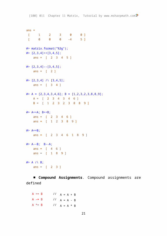
#> matrix.format("%3g");#> [2,3,4]++[3,4,5]; ans = [ 2 3 4 5 ]

#> [2,3,4]--[3,4,5]; ans = [ 2 ]

#> [2,3,4] /\ [3,4,5]; ans = [ 3 4 ]

#> A = [2,3,4,3,4,6]; B = [1,2,3,2,3,8,8,9]; A = [ 2 3 4 3 4 6 ] B = [ 1 2 3 2 3 8 8 9 ]

#> A++A; B++B; ans = [ 2 3 4 6 ]

15



ans = [ 1 2 3 8 9 ]

#> A++B; ans = [ 2 3 4 6 1 8 9 ]

#> A--B; B--A; ans = [ 4 6 ] ans = [ 1 8 9 ]

#> A /\ B; ans = [ 2 3 ]

■ Compound Assignments. Compound assignments are defined

A += B // A = A + BA -= B // A = A - BA *= B // A = A * BA /= B // A = A / BA |= B // A = A | B , horizontal concatenation (see below)A _= B // A = A _ B , vertical concatenation (see below)

A \_= B // A = A \_ B, diagonal concatenation

A += s // A = A + sA -= s // A = A - sA *= s // A = A * sA /= s // A = A / sA ^= s // A = A ^ s

A .*= B // A = A .* BA ./= B // A = A ./ BA .^= B // A = A .^ BA .^= s // A = A .^ s

A ++= B // A = A ++ B, set union A --= B // A = A -- B, set difference A /\= B // A = A /\ B, set intersection

where the dimensions must comply with the rules of relevant operations.

#> A = B = [ 1,2,3; 4,5,6 ]; A = [ 1 2 3 ]

16



[ 4 5 6 ]

#> A .^= 3 ; // A = A .^ 3 A = [ 1 8 27 ] [ 64 125 216 ]

#> A ./= B ; // A = A ./ B A = [ 1 4 9 ] [ 16 25 36 ]

#> A |= B; // A = A | B A = [ 1 8 27 1 2 3 ] [ 64 125 216 4 5 6 ]

#> A _= B; // A = A _ B A = [ 1 8 27 1 2 3 ] [ 64 125 216 4 5 6 ] [ 1 2 3 0 0 0 ] [ 4 5 6 0 0 0 ]

#> A = [ 1,2,3,5,9 ]; A = [ 1 2 3 5 9 ]

#> A --= [ 2,3,5,8,10 ]; // A = A -- [2,3,5,8,10] A = [ 1 9 ]

#> A ++= [ 3,4,17 ]; // A = A ++ [ 3,4,17 ] A = [ 1 9 3 4 17 ]

#> A /\= [ 3,4,21,23 ]; // A = A /\ [ 3,4,21,23 ] A = [ 3 4 ]

■ Vector Treatment. Any matrix of dimension m× n can be treated as a row vector of dimension 1 ×mn with columnwise counting by the syntax

A() // matrix of dimension 1 ×mn

In doing this, reading and writing are discriminated in that the final dimensions are different.

17



Reading of ‘A()’ creates an 1 ×mn matrix, for example

%> A(), 1 x mn matrix #> A = [ 1-1!,2-2!; 3-3!,4-4! ];#> A();A = [ 1 - i 1 2 - i 2 ] [ 3 - i 3 4 - i 4 ] ans = [ 1 - i 1 3 - i 3 2 - i 2 4 - i 4 ]

Meanwhile, writing via ‘A()’ preserves the dimension of ‘A’, and the data is accepted as a columnwise one-dimensional array.

Compound operations for A() are defined on an element-by-element base

A() += B // a_k += b_k, columnwise countingA() -= B // a_k -= b_kA() *= B // a_k *= b_k, equal to A .*= BA() /= B // a_k /= b_k, equal to A ./= BA() ^= B // a_k ^= b_k, equal to A .^= B

An example is as follows.

%> dimension-preserving compound operations #> X = [ 11:13; 21:23 ] ;#> Y = [ 1,4,7; 2,5,8; 3,6,9 ];X = [ 11 12 13 ] [ 21 22 23 ] Y = [ 1 4 7 ] [ 2 5 8 ] [ 3 6 9 ]

#> A = X;; A() *= Y;; A ; A = [ 11 36 65 ] // 11 * 1 12 * 3 13 * 5 [ 42 88 138 ] // 21 * 2 22 * 4 23 * 6

#> X() = [ -99,-88 ] ; // no change in dimension X =

18



[ -99 12 13 ] [ -88 22 23 ]

Section 11-4 Relational and Conditional Operations

Relational and conditional operations result in either ‘true’ or ‘false’, where either 1 or 0 is assigned to ‘true’ and ‘false’ , respectively.

■ ?: Ternary Operation. The ternary operation ‘?:’ in C is also available in Cemmath, especially for ‘double’ data. The syntax is

x ? a : b // a if x is true (i.e., not zero), otherwise b


%> ? : ternary operation#> 1 ? 2 : 3;ans = 2

#> 0 ? 2 : 3;ans = 3

■ Conditional Operations. Conditional operations are

A.all // 0 if any a_ij is zero, column-first operation A.any // 1 if any a_ij is not zero, column-first operation A.all1 // double-returning, equivalent to A.all.all(1)

A.any1 // double-returning, equivalent to A.any.any(1)

A && B // ( a_ij && b_ij ? 1 : 0 ) A || B // ( a_ij || b_ij ? 1 : 0 ) A !& B // ((a_ij && b_ij) || (!a_ij && !b_ij)) ? 1 : 0 ) A !| B // ((a_ij && !b_ij) || (!a_ij && b_ij)) ? 1 : 0 )

Example runs are

%> conditional operations#> A = [3,4; 0,0]; B = [1,0; 4,0];A = [ 3 4 ]

19



[ 0 0 ] B = [ 1 0 ] [ 4 0 ]

#> A && B ; // and ans = [ 1 0 ] [ 0 0 ]

#> A || B ; // or ans = [ 1 1 ] [ 1 0 ]

#> A !& B ; // exclusive andans = [ 1 0 ] [ 0 1 ]

#> A !| B ; // exclusive orans = [ 0 1 ] [ 1 0 ]

#> A.any ; ans = [ 1 1 ]

#> A.all; ans = [ 0 0 ]

#> A.any.any; A.any1 ; // A.any.any(1); ans = [ 1 ] ans = 1

#> A.all.all; A.all1 ; // A.all.all(1); ans = [ 0 ] ans = 0

Note that both ‘all1’ and ‘any1’ return ‘double’, while both ‘all’ and ‘any’ return ‘matrix’.

20



■ Relational Operations. Relational operations are defined for the following cases (A,B are matrices, s is double, z is complex)

A == B,s,z A != B,s,zA > B,sA < B,sA >= B,sA <= B,s

where all return matrices.

%> relational operations#> A = [3,4; 0,0];#> B = [1,0; 4,0]; A = [ 3 4 ] [ 0 0 ]

B = [ 1 0 ] [ 4 0 ]

#> A == B ; ans = [ 0 0 ] [ 0 1 ]

#> A != B ; ans = [ 1 1 ] [ 1 0 ]

#> A > B ; ans = [ 1 1 ] [ 0 0 ]

#> A >= B ; ans = [ 1 1 ]

21



[ 0 1 ]

#> A < B ; ans = [ 0 0 ] [ 1 0 ]

#> A <= B ; ans = [ 0 0 ] [ 1 1 ]

Note that ‘complex’ is applicable to both ‘==’ and ‘!=’ only.

If two matrices are of equal dimension m× n, operation A .mn. B returns true, otherwise returns false. The equality of two matices is examined by ‘A.eq.B’. The following binary operations return either 1 or 0 (true of false).

A .mn. B // size comparing

A .eq. B, s // true if all elements are equal A .ne. B, s // true if all elements are not-equal A .lt. B, s A .gt. B, s A .le. B, s A .ge. B, s

%> relational operations, true or false#> x = [ -2,3,4 ];; y = [ 1,3,5 ];;

#> x .mn. y ; // size comparingans = 1

#> x .eq. y ; ans = 0#> x .ne. y ; ans = 0#> x .lt. y ; ans = 0#> x .gt. y ; ans = 0#> x .le. y ; ans = 1#> x .ge. y ; ans = 0

#> x.eq.4 ; ans = 0#> x.ne.4 ; ans = 0#> x.lt.4 ; ans = 0

22



#> x.gt.4 ; ans = 0#> x.le.4 ; ans = 1#> x.ge.4 ; ans = 0

Section 11-5 Special Binary Operations

A ._ n // reshape in n-columns, equal to A.wide(n)

A ** B // A∗¿B=. ˙( A , B )= ∑k=1

min ( mn, pq )

ak bk

A ^^ B // Kronecker product, A ^^ B = .kron(A,B) A | B // horizontal concatenation, A | B = .horzcat(A,B) A _ B // vertical concatenation, A _ B = .vertcat(A,B)

A ++ B // set union, [2,3,4]++[3,4,5] = [2,3,4,5] A -- B // set difference, [2,3,4]--[3,4,5] = [2] A /\ B // set intersection, [2,3,4] /\ [3,4,5] = [3,4]

■ Dot and Cross Product. A dot product of m× n matrix A=(ak) and

p ×q matrix B=(bk) returns a scalar

A∗¿B=. ˙( A , B )= ∑k=1

min ( mn, pq)

ak bk

But the cross product works only with 3×1 or 1 ×3 matrices and returns a column vector

. cross ( A , B )=[a2b3−a3b2

a3 b1−a1b3

a1 b2−b2a1]

%> dot and cross#> A = (1:4)._2; B = (1:9)._3;A = [ 1 3 ] [ 2 4 ] B =

23



[ 1 4 7 ] [ 2 5 8 ] [ 3 6 9 ]

#> A**B; .dot(A,B) ; // 1*1 + 2*2 + 3*3 + 4*4ans = 30ans = 30

#> .cross( [2,1,5], [-1,2,4] ) ; ans = [ -6 -13 5 ]

■ Kronecker Product. A Kronecker product of m× n matrix A and p ×q

matrix B results in m× n block-matrix dimension of mp ×nq, and its (i , j)

block is a ij B. An example is

%> Kronecker product, A^^B = .kron(A,B)#> matrix.format("%6g") ;#> A = [ 1, 10, -100; -10, 1, 1000 ];; B = [ 1,2,3; 4,5,6; 7,8,9 ];;#> A ^^ B ;ans = [ 1 2 3 10 20 30 -100 -200 -300 ] [ 4 5 6 40 50 60 -400 -500 -600 ] [ 7 8 9 70 80 90 -700 -800 -900 ] [ -10 -20 -30 1 2 3 1000 2000 3000 ] [ -40 -50 -60 4 5 6 4000 5000 6000 ] [ -70 -80 -90 7 8 9 7000 8000 9000 ]

Cemmath extends the concept of the Kronecker product to handle various operatations more than multiplication via the upgraded function. For example, the above result is the same as

#> matrix kron2(double x) = x * [ 1, 10, -100; -10, 1, 1000 ] ;#> B = [ 1,2,3; 4,5,6; 7,8,9 ];; #> kron2++(B); // upgraded matrix(double) ans = [ 1 2 3 10 20 30 -100 -200 -300 ] [ 4 5 6 40 50 60 -400 -500 -600 ] [ 7 8 9 70 80 90 -700 -800 -900 ] [ -10 -20 -30 1 2 3 1000 2000 3000 ] [ -40 -50 -60 4 5 6 4000 5000 6000 ] [ -70 -80 -90 7 8 9 7000 8000 9000 ]

24



Another example is

#> matrix.format("%9g");#> matrix kron3(double x) = [ x, 1, -sqrt(x); 0, x^2, log(x) ] ; #> kron3++( [2,3;4,5] ); // upgraded matrix(double) ans = [ 2 3 1 1 -1.41421 -1.73205 ] [ 4 5 1 1 -2 -2.23607 ] [ 0 0 4 9 0.693147 1.09861 ] [ 0 0 16 25 1.38629 1.60944 ]

■ Horizontal Concatenation, A∨B. Two matrices can be horizontally concatenated by A∨B or .horzcat(A,B).

%> horizontal concatenation, A | B = .horzcat(A,B)#> A = [1,1; 1,1];; b = [3;6;9];; c = [3];;#> A|b; // longer b ans = [ 1 1 3 ] [ 1 1 6 ] [ 0 0 9 ]

#> A|c; // shorter c ans = [ 1 1 3 ] [ 1 1 0 ]

#> A|7; // constant ans = [ 1 1 7 ] [ 1 1 7 ]

■ Vertical Concatenation, AB. Two matrices can be vertically concatenated by AB or .vertcat(A,B). But care should be taken that '_' is seperated by spaces.

%> vertical concatenation, A _ B = .vertcat(A,B)#> A = [ 1,1; 1,1 ];; b = [ 3,6,9 ];; c = [ 3 ];;

#> A _ b; // longer b ans = [ 1 1 0 ] [ 1 1 0 ]

25



[ 3 6 9 ]

#> A _ c ; // shorter c ans = [ 1 1 ] [ 1 1 ] [ 3 0 ]

#> A _ 3 ; // constant ans = [ 1 1 ] [ 1 1 ] [ 3 3 ]

■ Diagonal Concatenation, A ¿B. Two matrices can be diagonally concatenated.

#> [ 1,2; 3,4 ] \_ [ 7-8i, 2; 5 ]; x = [ 1 2 0 0 ] [ 3 4 0 0 ] [ 0 0 7 - i 8 2 ] [ 0 0 5 0 ]#> x = []; x = []#> x \_= [1,2;3,4]; x = [ 1 2 ] [ 3 4 ]#> x \_= 5; x = [ 1 2 0 ] [ 3 4 0 ] [ 0 0 5 ]#> x \_= [ 11,12; 13,14; 15,16 ]; x = [ 1 2 0 0 0 ] [ 3 4 0 0 0 ] [ 0 0 5 0 0 ] [ 0 0 0 11 12 ] [ 0 0 0 13 14 ] [ 0 0 0 15 16 ]#> x \_= 7-8i; x =

26



[ 1 2 0 0 0 0 ] [ 3 4 0 0 0 0 ] [ 0 0 5 0 0 0 ] [ 0 0 0 11 12 0 ] [ 0 0 0 13 14 0 ] [ 0 0 0 15 16 0 ] [ 0 0 0 0 0 7 - i 8 ]

■ Block-Diagonal Matrices. A syntax

diagcat(...) .blkdiag( … )

creates a block-diagonal matrix. An example is as follows

%> block-diagonal matrix #> .diagcat( 5,6,7,8 );ans =

[ 5 0 0 0 ] [ 0 6 0 0 ] [ 0 0 7 0 ] [ 0 0 0 8 ]

#> .diagcat ( [1,2;3,4], 5, [11,13; 12,14] ); ans =

[ 1 2 0 0 0 ] [ 3 4 0 0 0 ]

[ 0 0 5 0 0 ] [ 0 0 0 11 13 ] [ 0 0 0 12 14 ]

#> .diagcat ( 2*.I(2), .ones(2) ); ans =

[ 2 0 0 0 ] [ 0 2 0 0 ] [ 0 0 1 1 ] [ 0 0 1 1 ]

■ Priorities of Operations. Priorities are listed from the highest.

A( ) A{ } A[ ] A. A..(rows)(columns) // highest|A| // absolute^ .^ // power, outer-product

27



!A ~A +A -A A! A` A' A.' A~ ++A // prefix, postfix* / \ .* ./ .\ A**B A^^B // multiplicative+ - // additive(A | B) (A _ B) (A \_ B) // concatenation< > <= >= .lt. .gt. .le. .ge. // relational== != .mn. .eq. .ne. // relational&& !& A /\ B // conditional, set|| !| A++B A--B // conditional, set= += -= *= /= ^= |= _= \_= // assignment

.*= ./= .^= ++= --= /\= , // comma, lowest

#> A = [ 1,2; 3,4 ]; A = [ 1 2 ] [ 3 4 ]

#> -A.^2 ; // -(A.^2), .^ is of higher priority ans = [ -1 -4 ] [ -9 -16 ]

Section 11-6 Rows, Columns and Diagonals

■ Diagonal Matrices. A syntax

.diag(A,k=0) or A.diagm(k)

creates a diagonal matrix from a matrix argument, where A is a matrix. An example is as follows

%> diagonal matrix#> .diag( [1,2,3,4] ); // [1,2,3,4].diagm(0);ans = [ 1 0 0 0 ] [ 0 2 0 0 ] [ 0 0 3 0 ] [ 0 0 0 4 ]

#> .diag( [1,2], 1 ); // [1,2].diagm(1);ans =

28



[ 0 1 0 ] [ 0 0 2 ] [ 0 0 0 ]

#> .diag( [3,4], -2 ); // [3,4].diagm(-2);ans =

[ 0 0 0 0 ] [ 0 0 0 0 ] [ 3 0 0 0 ] [ 0 4 0 0 ]

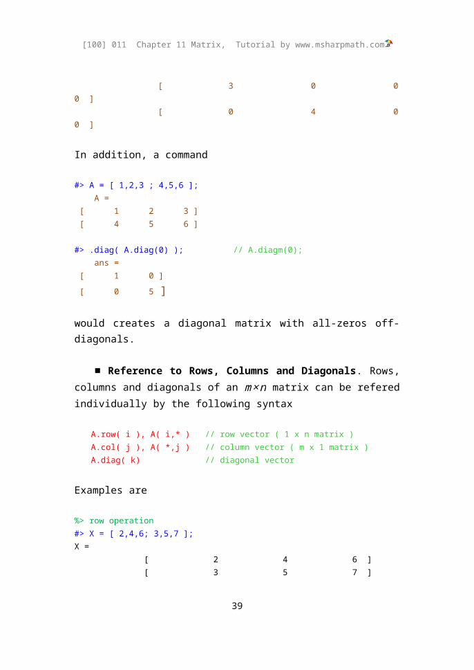
In addition, a command

#> A = [ 1,2,3 ; 4,5,6 ]; A = [ 1 2 3 ] [ 4 5 6 ]

#> .diag( A.diag(0) ); // A.diagm(0); ans = [ 1 0 ] [ 0 5 ]

would creates a diagonal matrix with all-zeros off-diagonals.

■ Reference to Rows, Columns and Diagonals. Rows, columns and diagonals of an m× n matrix can be refered individually by the following syntax

A.row( i ), A( i,* ) // row vector ( 1 x n matrix )A.col( j ), A( *,j ) // column vector ( m x 1 matrix )A.diag( k) // diagonal vector

Examples are

%> row operation#> X = [ 2,4,6; 3,5,7 ];X = [ 2 4 6 ] [ 3 5 7 ]

#> A = X;; A.row(2) *= 100:110 ; // A.row(i)

29



A = [ 2 4 6 ] [ 300 505 714 ]

■ Diagonal Vectors. For a special case of 3×5 matrix,

A=[a11 a12 a13 a14 a15

a21 a22 a23 a24 a25

a31 a32 a33 a35 a35]

diagonals are defined

A . diag ( k≤−2 )=[a31] , A . diag (−1 )=[a21

a32 ]A . diag (0 )=[a11

a22

a33] , A .diag (1)=[a12

a23

a34]

A . diag (2 )=[a13

a24

a35] , A . diag (3 )=[a14

a25]A . diag ( k≥ 4 )= [a15 ]

A . diagm (0 )=[a11 0 00 a22 00 0 a33

]For example, an eigenvalue-shifted matrix A−λ I can be calculated by

%> diagonal operation#> A = [ 2,5,8; 3,6,9; 4,7,10 ];A =

[ 2 5 8 ] [ 3 6 9 ] [ 4 7 10 ]

#> A.diag(0) -= 20;A =

30



[ -18 5 8 ] [ 3 -14 9 ] [ 4 7 -10 ]

#> A.diagm(0);ans = [ -18 0 0 ] [ 0 -14 0 ] [ 0 0 -10 ]

■ Deleting Row and Column. Deleting a single row and a single column can be carried out by the syntax

A.rowdel(i) // row delete, read onlyA.coldel(j) // column delete, read only

A.row(i) = []; // A = A.rowdel(i)A.col(j) = []; // A = A.coldel(j)

where ‘[]’ represent a null matrix. An example is

%> deleting row and column#> A = [ 11,12,13,14; 21,22,23,24; 31,32,33,34 ];A = [ 11 12 13 14 ] [ 21 22 23 24 ] [ 31 32 33 34 ]

#> A.row(2) = []; // equivalent to A = A.rowdel(2)A = [ 11 12 13 14 ] [ 31 32 33 34 ]

#> A.col(3) = []; // equivalent to A = A.coldel(3)A = [ 11 12 14 ] [ 31 32 34 ]

In general, deleting i-th row and j-th column from a matrix A results in a minor

denoted by Aij. The member function ‘minor’ is used to create a minor

%> minor#> A = [ 11,12,13,14; 21,22,23,24; 31,32,33,34 ];

31



A = [ 11 12 13 14 ] [ 21 22 23 24 ] [ 31 32 33 34 ]

#> A.minor(2,3); // equivalent to A.rowdel(2).coldel(3);ans = [ 11 12 14 ] [ 31 32 34 ]

Deleting a multiple number of rows and columns requires a concept of submatrices and is addressed in the following section.

■ Resizing, extending and inserting matrices. A matrix can be resized while keeping its elemenents.

A .resize(m,n) // a new dimesion m x n while copyingA .ext(m,n,x) // extend m rows, n columns and assign xA .insrow(i,B) // row insert, A.rowinsA .inscol(j,B) // column insert, A.colinsA .ins(i,j,B) // insert matrix at (i,j), A.insert

■ Resizing matrices. A matrix can be resized while keeping its elemenents. Note that resizing copies the original matrix only within a new dimension.

A .resize(m,n) // a new dimesion m x n while copying

#> A = [ 1,2,3; 4,5,6 ]; A = [ 1 2 3 ] [ 4 5 6 ]#> A.resize(4,6); ans = [ 1 2 3 0 0 0 ] [ 4 5 6 0 0 0 ] [ 0 0 0 0 0 0 ] [ 0 0 0 0 0 0 ]#> A.resize(4,2); ans = [ 1 2 ] [ 4 5 ] [ 0 0 ] [ 0 0 ]#> A.resize(1,5);

32



ans = [ 1 2 3 0 0 ]

■ Extending matrices. A matrix can be extended by additional rows and columns by

A .ext(m,n,x) // extend m rows, n columns and assign x

//----------------------------------------------------------------------#> matrix.format("%6g");#> A = (1:16)._4;A =[ 1 5 9 13 ][ 2 6 10 14 ][ 3 7 11 15 ][ 4 8 12 16 ]

#> A.ext(3,4, 0.); ans =[ 1 5 9 13 0 0 0 0 ][ 2 6 10 14 0 0 0 0 ][ 3 7 11 15 0 0 0 0 ][ 4 8 12 16 0 0 0 0 ][ 0 0 0 0 0 0 0 0 ][ 0 0 0 0 0 0 0 0 ][ 0 0 0 0 0 0 0 0 ]

■ Inserting matrices. Inserting matrices can be done in a number of ways.

A .insrow(i,B) // row insert, A.rowinsA .inscol(j,B) // column insert, A.colinsA .ins(i,j,B) // insert matrix at (i,j), A.insert

//----------------------------------------------------------------------#> matrix.format("%6g");#> A = (1:16)._4;A =[ 1 5 9 13 ][ 2 6 10 14 ][ 3 7 11 15 ][ 4 8 12 16 ]

//----------------------------------------------------------------------#> A.inscol(1, [101:105; 201:205]); // starts at column 1ans =[ 101 102 103 104 105 1 5 9 13 ]

33



[ 201 202 203 204 205 2 6 10 14 ][ 0 0 0 0 0 3 7 11 15 ][ 0 0 0 0 0 4 8 12 16 ]

#> A.inscol(2, [101:105; 201:205]'); // column 2ans =[ 1 101 201 5 9 13 ][ 2 102 202 6 10 14 ][ 3 103 203 7 11 15 ][ 4 104 204 8 12 16 ][ 0 105 205 0 0 0 ]

#> A.inscol(100, [101:105; 201:205]'); // out of range makes attachingans =[ 1 5 9 13 101 201 ][ 2 6 10 14 102 202 ][ 3 7 11 15 103 203 ][ 4 8 12 16 104 204 ][ 0 0 0 0 105 205 ]

//----------------------------------------------------------------------#> A.insrow(1, [101:105; 201:205]);ans =[ 101 102 103 104 105 ][ 201 202 203 204 205 ][ 1 5 9 13 0 ][ 2 6 10 14 0 ][ 3 7 11 15 0 ][ 4 8 12 16 0 ]

#> A.insrow(2, [101:105; 201:205]');ans =[ 1 5 9 13 ][ 101 201 0 0 ][ 102 202 0 0 ][ 103 203 0 0 ][ 104 204 0 0 ][ 105 205 0 0 ][ 2 6 10 14 ][ 3 7 11 15 ][ 4 8 12 16 ]

#> A.insrow(100, [101:105; 201:205]');ans =[ 1 5 9 13 ][ 2 6 10 14 ]

34



[ 3 7 11 15 ][ 4 8 12 16 ][ 101 201 0 0 ][ 102 202 0 0 ][ 103 203 0 0 ][ 104 204 0 0 ][ 105 205 0 0 ]

//----------------------------------------------------------------------#> A.ins(1,1, [101:105; 201:205]); // [101:105; 201:205] \_ A ans =[ 101 102 103 104 105 0 0 0 0 ][ 201 202 203 204 205 0 0 0 0 ][ 0 0 0 0 0 1 5 9 13 ][ 0 0 0 0 0 2 6 10 14 ][ 0 0 0 0 0 3 7 11 15 ][ 0 0 0 0 0 4 8 12 16 ]

#> A.ins(2,2, [101:105; 201:205]');ans =[ 1 0 0 5 9 13 ][ 0 101 201 0 0 0 ][ 0 102 202 0 0 0 ][ 0 103 203 0 0 0 ][ 0 104 204 0 0 0 ][ 0 105 205 0 0 0 ][ 2 0 0 6 10 14 ][ 3 0 0 7 11 15 ][ 4 0 0 8 12 16 ]

#> A.ins(100,100, [101:105; 201:205]'); // A \_ [101:105; 201:205]'ans =[ 1 5 9 13 0 0 ][ 2 6 10 14 0 0 ][ 3 7 11 15 0 0 ][ 4 8 12 16 0 0 ][ 0 0 0 0 101 201 ][ 0 0 0 0 102 202 ][ 0 0 0 0 103 203 ][ 0 0 0 0 104 204 ][ 0 0 0 0 105 205 ]

Section 11-7 Submatrices

35



■ Real and Imaginary Parts. For a complex matrix A=X+iY , the real part

X

and the imaginary part Y

are denoted by

A.real // real part X=( x ij ) of A=X+iYA.imag // imaginary part Y=( y ij ) of A=X+iY

respectively. Note that ‘A = A.real + i A.imag’. Whether a matrix is real or complex can be found by the syntax

A.isreal // returns 1 if A is real, otherwise return 0

The real and imaginary parts can be modified as a whole

%> real/imaginary matrix#> A = [ 1-1!, 3-3!; 2-2!, 4-4! ];A = [ 1 - i 1 3 - i 3 ] [ 2 - i 2 4 - i 4 ]

#> A.real = 10:15;; A; // in one-dimensional senseA = [ 10 - i 1 12 - i 3 ] [ 11 - i 2 13 - i 4 ]

#> A.imag = 100;; A; // modifying imaginary matrixA = [ 10 + i 100 12 + i 100 ] [ 11 + i 100 13 + i 100 ]

■ Syntax for Entry of Elements. Let us consider a 3× 4 matrix A written as

A=[a1 a4 a7 a10

a2 a5 a8 a11

a3 a6 a9 a12]

Then, a set of elements for A can be defined by the following syntax

36



A.(matrix) // entry of elementsA.entry(matrix) // entry of elements

An example is

A . ( [ 2,6,10 ] )≡[ a2

a6

a10] , A . entry ( [ 8,3,11,5 ]) ≡[ a8

a3

a11

a5]

and the corresponding Cemmath commands are

%> entry of elements#> A = [ 1,4,7,10; 2,5,8,11; 3,6,9,12 ]*10; A = [ 10 40 70 100 ] [ 20 50 80 110 ] [ 30 60 90 120 ] #> A.([2,6,10]); ans = [ 20 60 100 ]

#> A.entry([8,3,11,5]); ans = [ 80 30 110 50 ]

Compound operations with regard to the member function ‘entry’ are defined. Examples are

%> compound operation with entry#> A = [ 1,4,7,10; 2,5,8,11; 3,6,9,12 ] * 10;A = [ 10 40 70 100 ] [ 20 50 80 110 ] [ 30 60 90 120 ]

#> A.( [12,6,8,1] ) += 100:800:100; // A.( ) = A.entry( )A = [ 410 40 70 100 ] [ 20 50 380 110 ] [ 30 260 90 220 ]

37



One interesting performance of ‘A.(B) or A.entry(B)’ occurs when the matrix B=( bk ) has a dimension equal to or greater than the matrix A=(ak ).

In this case, ak is selected for any bk ≠ 0. For example,

A=[a1 a3 a5

a2 a4 a6] , B=[0 ,3 ,0.1 ,−2, 0 , 1]

results in

%> compound operation with entry#> A = [ 10,30,50; 20,40,60 ];#> B = [ 0, 3, 0.1, -2,0,1 ]; A = [ 10 30 50 ] [ 20 40 60 ] B = [ 0 3 0.1 -2 0 1 ]

#> A.(B); // A.entry(B) ans = [ 20 30 40 60 ]

Note that both a1 and a5 have not been selected sinceb1=b5=0.

■ Syntax for Submatrices. For ease of explanation, let us consider a 3× 4 matrix A written as

A=[a11 a12 a13 a14

a21 a22 a23 a24

a31 a32 a33 a34]

Then, a submatrix of A can be defined by two sets of indices, one is for rows and and the other is for columns. The syntax becomes

// double dots .. correspond to double parentheses ()()A..( rows )( columns ) // submatrixA.sub( rows )( columns ) // submatrix

where a star ‘*’ or a blank pair () can replace all rows or all columns. In this

38



regard, it can be noted that

A..(i)() is equivalent to A.row(i) or A(i,*)A..()(j) is equivalent to A.col(j) or A(*,j)

Also, one thing worthy of note is that counting is always done columnwise, and direction is important. For example,

A .. (2 ) (2,4,3 )=[a22 a24 a23]

A .. (2 ) ( 4,2,3 )=[a24 a22 a23 ]

A .. () (2,3 )=[a12 a13

a22 a23

a32 a33]

A ..(3,2)()=[a31 a32 a33 a34

a21 a22 a23 a24 ]A .. (1,3 ) (3,1 )=[a13 a11

a33 a31]A .. (3,1 ) ( 4 :2 )=[a34 a33 a32

a14 a13 a12 ]A .. (3,1 ) (2 :4 )=[a32 a33 a34

a12 a13 a14 ]A .. (1,3 ) ( 4 :2 )=[a14 a13 a12

a34 a33 a32 ]Assignment and compound assignments are defined for submatrices. An example is

%> direction of submatrix indexing

39



#> X = [ 1-1!,4-4!,7-7!; 2-2!,5-5!,8-8!; 3-3!,6-6!,9-9! ];X = [ 1 - i 1 4 - i 4 7 - i 7 ] [ 2 - i 2 5 - i 5 8 - i 8 ] [ 3 - i 3 6 - i 6 9 - i 9 ]

#> A = X;; A..(2,3)(2,3) += 100:110;A = [ 1 - i 1 4 - i 4 7 - i 7 ] [ 2 - i 2 105 - i 5 110 - i 8 ] [ 3 - i 3 107 - i 6 112 - i 9 ]

#> A = X;; A..(2,1)(2,3) *= 100:110;A = [ 1 - i 1 404 - i 404 721 - i 721 ] [ 2 - i 2 500 - i 500 816 - i 816 ] [ 3 - i 3 6 - i 6 9 - i 9 ]

■ Deleting Submatrices. Deleting all the elements in the submatrices is possible by the following syntax

A.subdel(rows)() // delete specified rows, read onlyA.subdel()(columns) // delete specified columns, read onlyA.subdel(rows)(columns) // delete rows and columns, read only

A..(rows)() = []; // same as A = A.subdel(rows)();A..()(columns) = []; // same as A = A.subdel()(columns);A..(rows)(columns) = []; // same as A = A.subdel(rows)(columns);

However, it should be remembered that the above syntax behaves similarly to the member function ‘minor’. For example, the following command

A..(i)(j) = [];

is the same as

A = A.minor(i,j);

Similarly, ‘A..(1,2,5)(2,4)=[]’ deletes rows ‘1,2,5’ and columns ‘2,4’ from the original matrix ‘A’. This can be confirmed by

%> deleting submatrices#> X = [ 11:14; 21:24; 31:34; 41:44; 51:54 ];

40



X = [ 11 12 13 14 ] [ 21 22 23 24 ] [ 31 32 33 34 ] [ 41 42 43 44 ] [ 51 52 53 54 ]

#> A = X;; A..(1,2,5)() = []; // equivalent to A = A.subdel(1,2,5)();A = [ 31 32 33 34 ] [ 41 42 43 44 ]

#> A = X;; A..()(2,4) = []; // equivalent to A = A.subdel()(2,4);A = [ 11 13 ] [ 21 23 ] [ 31 33 ] [ 41 43 ] [ 51 53 ]

// equivalent to A = A.subdel(1,2,5)(2,4);#> A = X;; A..(1,2,5)(2,4) = [];A = [ 31 33 ] [ 41 43 ]

■ Function ‘true’ and ‘false’. A member function ‘true’ or ‘find’ retrieves a set of subscripts corresponding to nonzero elements. On the other hand, a member function ‘false’ retrieves a set of subscripts corresponding to zero elements. For example,

%> nonzero/zero-element index#> X = [ -2,3,0;-4,0,0;0,0,0 ]; X = [ -2 3 0 ] [ -4 0 0 ] [ 0 0 0 ]

#> X.true; // X .find ans = [ 1 2 4 ]

#> X.false; ans = [ 3 5 6 7 8 9 ]

Together with the member function ‘entry’, member function ‘true’ is

41



used to construct a new matrix. Example runs are presented below.

%> nonzero-element index#> A = X = [ 1,2,3; 2,-3,4 ]; B = [ -1,-2,4; 3,2,1 ]; A = [ 1 2 3 ] [ 2 -3 4 ] B = [ -1 -2 4 ] [ 3 2 1 ]

#> f = ( A < B ).true ; f = [ 2 4 5 ]

#> A = X;; A.( f ); ans = [ 2 -3 3 ]

#> A = X;; A.( f ) = 0; A = [ 1 2 0 ] [ 0 0 4 ]

#> A = X;; A.( A < B ) += 1! ; A = [ 1 2 3 + i 1 ] [ 2 + i 1 -3 + i 1 4 ]

Section 11-8 ‘figure’ Related Functions

//----------------------------------------------------------------------// 'figure'-Returning Functions//----------------------------------------------------------------------A .plot // plotA .splplot // plot piecewise polynomials

//----------------------------------------------------------------------// piecewise polynomials//----------------------------------------------------------------------Piecewise continuous polynomials are defined with a number of polynomials and corresponding intervals

x11 ≤ x ≤ x12 : p1 ( x )=a10+a11 x+a12 x2+…+a1 n xn+…

42



x21≤ x≤ x22 : p2 ( x )=a20+a21 x+a22 x2+…+a2n xn+…⋮

xm 1≤ x≤ xm2: pm ( x )=am0+am1 x+am2 x2+…+amn xn+…

Combination of these piecewise polynomials can be expressed by the following matrix

A=[ x11 x12 a10 a11 ⋯x21 x22 a20 a21 ⋯⋮ ⋮ ⋮ ⋮ ⋮

xm1 xm2 am 0 am1 ⋯ ]This special representation by a matrix can be handled in various ways

A.spl(x) // evaluation for double A.spl(B) // evaluation for matrix A.spldiff // differentiate piecewise polynomials A.splint // integrate piecewise polynomials A.splplot ; // plot piecewise polynomials

#> x = (0:9).tr; #> [ x, x+1, x+1 ].splplot; // spline plot

Data set {( x1 , y1) , ( x2 , y2 ) ,…, ( xn, yn )} can be connected by lines and represented by piecewise continuous polynomials as follows.

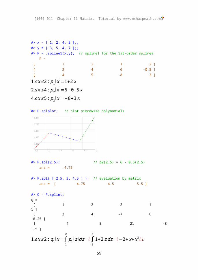
#> x = [ 1, 2, 4, 5 ];; #> y = [ 3, 5, 4, 7 ];;

43



#> P = .spline1(x,y); // spline1 for the 1st-order splines P = [ 1 2 1 2 ] [ 2 4 6 -0.5 ] [ 4 5 -8 3 ]

1 ≤ x ≤2 : p1 ( x )=1+2 x2 ≤ x ≤ 4 : p2 (x )=6−0.5 x4 ≤ x ≤5 : p3 ( x )=−8+3 x

#> P.splplot; // plot piecewise polynomials

#> P.spl(2.5); // p2(2.5) = 6 - 0.5(2.5) ans = 4.75

#> P.spl( [ 2.5, 3, 4.5 ] ); // evaluation by matrix ans = [ 4.75 4.5 5.5 ]

#> Q = P.splint; Q = [ 1 2 -2 1 1 ] [ 2 4 -7 6 -0.25 ] [ 4 5 21 -8 1.5 ]

1 ≤ x ≤2 :q1 ( x )=∫1

x

p1 (z ) dz=¿∫1

x

1+2 z dz=¿−2+x+x2 ¿¿

2 ≤ x ≤ 4 :q2 ( x )=∫2

x

p2 ( z )dz+q1 (2 )=−7+6 x− 14

x2

4 ≤ x ≤5 :q3 ( x )=∫4

x

p3 ( z ) dz+q2 (4 )=21−8 x+ 32

x2

#> Q.spl(4.5) - Q.spl(2.5); ans = 8.9375

44



∫2.5

4

p2 (x ) dx+∫4

4.5

p3 ( x ) dx=[−7+6 x−14

x2]2.5

4

+[21−8 x+32

x2]4

4.5

=8.9375

For spline interpolation using 3rd-degree polynomials, example is

#> x = [ 1, 2, 4, 5 ];; #> y = [ 3, 5, 4, 7 ];; #> P = .spline(x,y); // 1st and 2nd columns for interval P = [ 1 2 1 0.625 2.0625 -0.6875 ] [ 2 4 -10.5 17.875 -6.5625 0.75 ] [ 4 5 89.5 -57.125 12.1875 -0.8125 ]

1 ≤ x ≤2 : p1 ( x )=1+0.625 x+2.0625 x2−0.6875 x3

2≤ x ≤ 4 : p2 (x )=−10.5+17.875 x−6.5625 x2+0.75 x3

4 ≤ x ≤5 : p3 ( x )=89.5−57.125 x+12.1875 x2−0.8125 x3

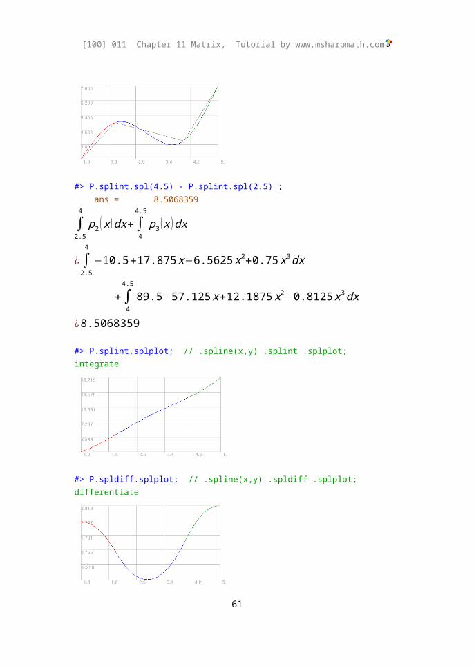
#> P.splplot; // .spline(x,y).splplot;#> [ x', y' ].plot+ ;

#> P.splint.spl(4.5) - P.splint.spl(2.5) ; ans = 8.5068359

∫2.5

4

p2 (x ) dx+∫4

4.5

p3 ( x ) dx

¿∫2.5

4

−10.5+17.875 x−6.5625 x2+0.75x3 dx

+∫4

4.5

89.5−57.125 x+12.1875 x2−0.8125 x3 dx

¿8.5068359

45



#> P.splint.splplot; // .spline(x,y) .splint .splplot; integrate

#> P.spldiff.splplot; // .spline(x,y) .spldiff .splplot; differentiate

Section 11-9 ‘matrix’-Returning Functions

A large number of member functions returning matrix are implemented in Cemmath. Therefore, this section describes ‘matrix’-returning functions.

■ Returning a Single Matrix. For ease of explanation, a 3 × 4

matrix

A=[a11 a12 a13 a14

a21 a22 a23 a24

a31 a32 a33 a34]=[a1 a4 a7 a10

a2 a5 a8 a11

a3 a6 a9 a12]

will be employed as a representative matrix for operations. In the above, both two-dimensional indexing and one-dimensional (columnwise) indexing are displayed for visual clarity of forthcoming operations.

For a complex element a ij=x ij+i y ij, its conjugate is defined as a ij=xij−i y ij. Then, a conjuage matrix is denoted by the member function ‘conj’

46



A=A . conj=[a1 a4 a7 a10

a2 a5 a8 a11

a3 a6 a9 a12]

It can be noted that the following member functions are self-explanatory from their names

A'=A .conjtr=[ a1 a2 a3

a4 a5 a6

a7 a8 a9

a10 a11 a12] , A . flipud=[a3 a6 a9 a12

a2 a5 a8 a11

a1 a4 a7 a10]

A . rot 90=[a10 a11 a12

a7 a8 a9

a4 a5 a6

a1 a2 a3] , A . rotm90=[ a3 a2 a1

a6 a5 a4

a9 a8 a7

a12 a11 a10]

A . triu (0 )=[a11 a12 a13 a14

0 a22 a23 a24

0 0 a33 a34] , A . tril(0)=[a11 0 0 0

a21 a22 0 0a31 a32 a33 0]

Listed below are a number of member functions returning a single matrix. More member functions are summarized in the last section.

A.inv // inverse matrixA.conj // ~A = A.conj, complex conjugateA.conjtr // A' = A.conjtr, conjugate transpose A.tr // A.' = A.tr, transpose A.chol // Choleski decomposition

A.rot90 // rotate 90 degree (counter-clockwise)A.rotm90 // rotate -90 degreeA.rev // reverse elements A.flipud // reverse rows, flip upside-downA.fliplr // reverse columns, flip left-right

47



A.wide(n) // A._n = A.wide(n), reshape in n-columns A.high(m) // reshape in m-rowsA.triu(k) // upper-triangular A.tril(k) // lower-triangularA.skewu(k) // upper-triangular w.r.t the skew-diagonalA.skewl(k) // lower-triangular w.r.t the skew-diagonal

A.pushu // push-up with bottom rowA.pushd // push-down with top rowA.pushl // push-left with rightmost columnA.pushr // push-right with leftmost column

A.pm // (-1)^(i+j) a_ijA.trun(eps=1.e-30) // truncate elements

A.trun1, ... ,trun16 // truncate with ϵ=10−1 ,10−2, …, 10−16 A.ratio(denom=10000) // shows a rational approximationA.rowswap(i,j) // A.swap = A.rowswap, swap i-th and j-th rows A.colswap(i,j) // swap i-th and j-th columns

A.repmat(m,n=m) // repeat a tile-shaped copyingA.minor(i,j) // minor generated by eliminating i-th and j-th

A.round // the closest interger for each elementA.decimal // deviation from closest interger for each element

A.backsub // backward substitution A.forsub // forward substitutionA.gausselim // Gauss-elimination without pivotA.gaussjord // Gauss-Jordan elimination with pivotA.gausspivot // Gauss elimination with pivot A.fact // element-by-element factorial, ( aij ! )A.dfact // element-by-element double factorial, ( aij ‼ )A.eigvec(lam) // eigenvector corresponding to lam

For example, the member function ‘repmat(m,n=m)’ generates a tile-shaped copy

%> repmat, repeat a matrix#> A = .I(2).repmat(2); A = [ 1 0 1 0 ] [ 0 1 0 1 ] [ 1 0 1 0 ] [ 0 1 0 1 ]

48



Another example is presented with ‘triu’ and ‘tril’

%> triu, tril#> A = (1:12)._4; A = [ 1 4 7 10 ] [ 2 5 8 11 ] [ 3 6 9 12 ]

#> A.triu(1);ans = [ 0 4 7 10 ] [ 0 0 8 11 ] [ 0 0 0 12 ]

#> A.tril(1);ans = [ 1 4 0 0 ] [ 2 5 8 0 ] [ 3 6 9 12 ]

Section 11-10 ‘poly’ and ‘double’ Related Functions

In this section, member functions returning ‘poly’ and ‘double’ are discussed. Those member functions returning ‘matrix’ will be addressed in the following sections.

■ ‘poly’-Returning Functions. A few member functions are returning ‘poly’

A.eigpoly // eigenpolynomialA.dpoly // descending polynomialA.apoly // ascending polynomialA.roots // (x-x1)(x-x2)...(x-xn), equivalent to A.root

For example,

%> eigenpolynomial#> A = [ 3,2,4; 2,5; 1,-1,2 ];A = [ 3 2 4 ]

49



[ 2 5 0 ] [ 1 -1 2 ]

#> p = A.eigpoly; // p = x^3 - 10 x^2 + 23 x + 6p = poly( 6 23 -10 1 )

#> p[A]; // cf. p(A) is element-by-elementans = [ 0 0 0 ] [ 0 0 0 ] [ 0 0 0 ]

which shows that p ( x )=x3−10 x2+23 x+6 is the eigen polynomial of matrixA.

A few lower polynomials are displayed with information

#> [ 1,3,2 ].roots ; y = x^3 - 6x^2 + 11x - 6 roots [ 2 ] [ 3 ] [ 1 ] local maxima ( 1.42265, 0.3849 ) local minima ( 2.57735, -0.3849 ) inflection pt. ( 2, 0 ) y-axis intersect ( 0, -6 )

■ ‘double’-Returning Functions. For a matrix A of dimensionm× n, some member functions returning ‘double’ are as follows.

A.cond // condition number, A.norminf*A.inv.norminfA.det // determinantA.end // A(end,end), last real entry

A.i(k) // i-th row for k-th linear indexA.ipos(x) // A(i) <= x <= A(i+1) or A(i+1) <= x <= A(i)A.isreal // returns 1 if A is realA.issquare // returns 1 if A is square

A.j(k) // j-th column for k-th linear index A.k(i,j) // k = m(j-1)+i, linear index for (i,j)

A.len/length // max(m,n)A.longer // max(m,n)A.m // m, number of rows

50



A.max1 // A.max.max(1)A.min1 // A.min.min(1)A.max1k // linear index k for A.max.max(1)

A.min1k // linear index k for A.min.min(1) A.maxentry // absolute maximum entry

A.minentry // absolute minimum entryA.maxentryk // linear index k for absolute maximum entryA.minentryk // linear index k for absolute minimum entryA.mn // m*n, total number of elementsA.n // n, number of columns A.prod1 // A.prod.prod(1)A.rank // rank of a matrix AA.ratio1 // shows a denomenator of rational approximationA.shorter // min(m,n)A.sum1 // A.sum.sum(1)

A.trace // trace, ∑i=0

n

aii

Examples are

%> size-related#> A = (1:12)._4;A = [ 1 4 7 10 ] [ 2 5 8 11 ] [ 3 6 9 12 ]

#> A.longer ; ans = 4#> A.shorter ; ans = 3#> A.mn ; ans = 12#> A.m ; ans = 3#> A.n ; ans = 4

%> determinant, trace#> A = [ 3,2,5; 1,4,3; 5,1,2 ];A = [ 3 2 5 ] [ 1 4 3 ] [ 5 1 2 ]

#> A.det ; ans = -54#> A.trace ; ans = 9

51



%> rank of a matrix#> A = [ 1,2; -1,-2; 2,4 ]; A.rank; A = [ 1 2 ] [ -1 -2 ] [ 2 4 ] ans = 1

#> A = [ 1,-1,2; 2,-2,4 ]; A.rank; A = [ 1 -1 2 ] [ 2 -2 4 ] ans = 1

#> A = [ 1,-1,2; 2,-2,3 ]; A.rank; A = [ 1 -1 2 ] [ 2 -2 3 ] ans = 2

%> double-returning#> A = matrix.hilb(4);A = [ 1 0.5 0.33333 0.25 ] [ 0.5 0.33333 0.25 0.2 ] [ 0.33333 0.25 0.2 0.16667 ] [ 0.25 0.2 0.16667 0.14286 ]

#> A.ratio;ans = (1/420) x [ 420 210 140 105 ] [ 210 140 105 84 ] [ 140 105 84 70 ] [ 105 84 70 60 ]

#> A.ratio1;ans = 420

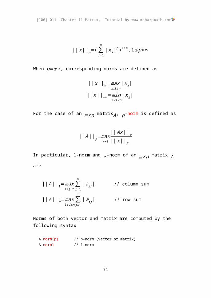
■ Norm of Matrix. A p-norm of an n-vector x is defined as

52



|| x | |p=(∑i=1

n

| xi |p )1 / p ,1 ≤ p<∞

When p=±∞, corresponding norms are defined as

|| x | |∞=max1 ≤i ≤n

| xi |

|| x | |−∞=min1 ≤i ≤n

| xi |

For the case of an m× n matrixA, p-norm is defined as

|| A | |p=maxx≠ 0

|| Ax | |p

|| x || p

In particular, 1-norm and ∞-norm of an m× n matrix A are

|| A | |1=max1≤ j≤ n

∑i=1

m

| aij | // column sum

|| A | |∞=max1 ≤ i≤ n

∑j=1

n

|aij | // row sum

Norms of both vector and matrix are computed by the following syntax

A.norm(p) // p-norm (vector or matrix)A.norm1 // 1-norm

A.norm2 // Frobenius norm, || A | |F=[∑i=1

m

∑j=1

n

|aij |2]

1 / 2

A.norm22 // A.norm22 = A.norm2^2 = A**A = .dot(A,A)A.norminf // infinite-norm

where the Frobenius norm is also included. Recalling that ‘A()’ is a vector derived from a matrix ‘A’, the Frobenius norm can be alternatively computed by

53



A().norm(p) // to compute || A | |F=[∑i=1

m

∑j=1

n

|aij |p]

1 / p

where p=2 is used.

Example runs are presented below.

%> norm1, norm2, norminf for vector#> x = 1:4;x = [ 1 2 3 4 ]

#> x.norm1; ans = 10#> x.norm2; ans = 5.4772256 // equivalent to x.norm(2) #> x.norminf; ans = 4 // equivalent to |x|.max1

%> norm1, norm2, norminf for matrix#> A = [ 1,2,3; 4,5,6; 7,8,9 ];A = [ 1 2 3 ] [ 4 5 6 ] [ 7 8 9 ]

#> A.norm1; ans = 18#> A.norm2; ans = 16.881943#> A.norminf; ans = 24#> A().norm(2); ans = 16.881943

Section 11-11 Several Useful Member Functions

■ Data-Processing Functions. All the data-processing functions listed below are always returning ‘matrix’ and perform column-first operations.

A.min // minimum elements A.max // maximum elements A.mean // mean elements A.std // standard deviation A.sum // sum of elements A.prod // product of elements A.diff // A` = A.diff, finite-difference

54



A.cumsum // A~ = A.cumsum, cumulative sum A.cumprod // cumulative productA.unit // normalize each column or 1-row matrix

Meanwhile, ‘double’-returning functions are

A.max1 // max a ij, equivalent to A.max.max(1)A.min1 // min aij, equivalent to A.min.min(1)A.sum1 // equivalent to A.sum.sum(1)A.prod1 // equivalent to A.prod.prod(1)

When the resulting scalar beomes ‘complex’, it is required to use ‘complex’-element such that ‘A.max.max[1]’. A few examples are discussed below.

%> max, min#> A = [ 0,-1,2; 1,2,-4; 5,-3,-4 ];A = [ 0 -1 2 ] [ 1 2 -4 ] [ 5 -3 -4 ]

#> A.max;ans = [ 5 2 2 ]

#> A.min;ans = [ 0 -3 -4 ]

// matrix, matrix, double, double#> A.max.max; A.min.min; A.max1; A.min1; ans = [ 5 ] ans = [ -4 ]ans = 5ans = -4

■ Useful Member Functions. Listed below are a few member functions important in linear algebra. In some cases, a multiple number of matrices can be returned by member functions. These cases can be handled by utilizing a matrix tuple, for example ‘(L,U)’ for LU-decomposition.

55



A.chol // Choleski decomposition A.eig // return a column vector for eigenvaluesA.hess // eigenvalue-preserving Hessenberg matrix

(i,j) = A.k(k) // linear index to row-column index(L,U) = A.lu // A = LU decomposition(Q,R) = A.qr // A = QR decomposition(P,L,U) = A.plu // A = PLU decomposition (m,n) = A.size // double tuple, number of rows and columns(X,D) = A.eig // modal and spectral matrices(lam,x) = A.eigpow(s) // largest eigenvalue by power method, shift s(lam,x) = A.eiginvpow(s) // smallest eigenvalue by inverse power method

For example, eigenvalue-preserving Hessenberg matrix can be illustrated by

%> eigenvalues and Hessenberg matrix#> A = [ 4,3,-2,1; 3,1,7,9; -2,7,5,4; 1,9,4,2 ];A = [ 4 3 -2 1 ] [ 3 1 7 9 ] [ -2 7 5 4 ] [ 1 9 4 2 ]

#> A.hess; ans =

[ 4 -3.74166 0 0 ] [ -3.74166 -1.07143 6.83441 8.88178e-016 ] [ 0 6.83441 7.29972 9.24686 ] [ 0 0 9.24686 1.77171 ]

#> A.hess.eig; ans =

[ 5.61943 ] [ -8.47695 ]

[ -1.2945 ] [ 16.152 ]

#> A.eig; ans =

[ 5.61943 ] [ -8.47695 ] [ -1.2945 ] [ 16.152 ]

56



#> (X,D) = A.eig; X = [ -795.08 356.977 239.519 283.71 ] [ -130.371 -1490.7 -61.736 1671.68 ] [ 394.046 515.734 366.777 1543.39 ] [ -108.369 1049.58 -349.371 1519.39 ]D = [ 5.61943 0 0 0 ] [ 0 -8.47695 0 0 ] [ 0 0 -1.2945 0 ] [ 0 0 0 16.152 ]

which show both the eigenvectors and eigenvalues.

■ Tensor-Related Functions. Rotation in the three-dimensional space can be expressed by specific orthogonal 3 ×3 matrices. For example, a stress tensor can be written as

σ=[ i j k ] [σ11 σ12 σ13

σ21 σ22 σ23

σ31 σ32 σ33][ i

jk ]

This stress tensor can be interpreted with respect to a rotated coordinate expressed as

[ ijk ]=Q [e1

e2

e3]

where Q is an orthogonal matrix. Then, it can be seen that

σ=[e1 e2 e3 ]QT [σ11 σ 12 σ13

σ21 σ 22 σ23

σ31 σ 32 σ33]Q [e1

e2

e3]

57



~S=QT [ σ11 σ12 σ 13

σ 21 σ22 σ 23

σ 31 σ32 σ 33]Q

which represents the Mohr’s circle in the continuum mechanics. For the above, Cemmath adopts the following six rotations of 3×3 matrices

A.xrot(theta) // rotation around the x-axisA.yrot(theta) // rotation around the y-axisA.zrot(theta) // rotation around the z-axis

A.xrotd(theta) // rotation around the x-axis (in degree)A.yrotd(theta) // rotation around the y-axis (in degree)A.zrotd(theta) // rotation around the z-axis (in degree)


%> zrotd #> X = [ 0,1,0; 1,0,0; 0,0,0 ]; // s = ( ij+ji ), pure shear#> X.zrotd(45).trun10; // snew = ( uu-vv ), tension and compressionX = [ 0 1 0 ] [ 1 0 0 ] [ 0 0 0 ] ans = [ 1 0 0 ] 0 -1 0 ] [ 0 0 0 ]

Section 11-12 Matrix Functions and Array of Matrices

■ Extension of Functions. Several mathematical functions such as 'sqrt' can be extended to apply to a matrix. For example, one may want to find a matrix X from the following equation

XX=A

which can be solved by

58



X=√ A

This is different from the element-by-element operation x ij=√aij, and thus a matrix function 'sqrtm' is implemented in Cemmath. For example,

#> A = [ 1,0.3; 0.2,1 ]; sqrt(A); X = sqrtm(A); A = [ 1 0.3 ] [ 0.2 1 ] ans = [ 1 0.547723 ] [ 0.447214 1 ] X = [ 0.992355 0.151156 ] [ 0.10077 0.992355 ]

#> X^2 ; ans = [ 1 0.3 ] [ 0.2 1 ]

Also, a sum of an infinite series and its inverse function

exp¿¿A=log (exp( A ))

are computed by 'expm' and 'logm', respectively.

#> A = [1,0.3; 0.2,1]; E = expm(A); L = logm(A); A = [ 1 0.3 ] [ 0.2 1 ] E = [ 2.80024 0.823664 ] [ 0.549109 2.80024 ] L = [ -0.0309377 0.306226 ] [ 0.20415 -0.0309377 ]

#> logm(E); ans = [ 1 0.3 ]

59



[ 0.2 1 ]

#> expm(L); ans = [ 1 0.3 ] [ 0.2 1 ]

Especially, expm(A) can be approximately computed by

#> p = poly(0:10).fact .inv;;#> p[A]; ans = [ 2.80024 0.823664 ] [ 0.549109 2.80024 ]

■ Array of Matrix. An array of matrices is defined according to the following syntax

matrix P[7],Q[21], … ;

where ‘P’ and ‘Q’ are the names of arrays. The dimension of an array can be a variable of type ‘double’. An example is presented below.

%> array #> matrix.format("%3g");#> n = 7;n = 7

#> matrix Ar[n];#> for.i(0,4) Ar[i] = .I(i+1);;#> Ar;Ar = matrix [7] [0] = [ 1 ] [1] = [ 1 0 ] [ 0 1 ] [2] = [ 1 0 0 ] [ 0 1 0 ] [ 0 0 1 ] [3] = [ 1 0 0 0 ]

60



[ 0 1 0 0 ] [ 0 0 1 0 ] [ 0 0 0 1 ] [4] = [ 1 0 0 0 0 ] [ 0 1 0 0 0 ] [ 0 0 1 0 0 ] [ 0 0 0 1 0 ] [ 0 0 0 0 1 ] [5] = [ undefined ] [6] = [ undefined ]

#> Ar[1];ans = [ 1 0 ] [ 0 1 ]

#> Ar[4].longer;ans = 5

#> Ar[5].len;ans = 0

Section 11-13 Special Matrices

■ Special matrices. In mathematics, there are a number of special matrices used for particular purposes. For example, the Hilbert matrix expressed as

a ij=1

i+ j−1, i=1,2 ,…, n , j=1,2,…,n

is used to illustrate ill-conditioned matrix. Some of the special matrices are created by class functions

matrix.hilb (long) // Hilbert matrixmatrix.hank (matrix,matrix) // hankel

matrix.toep (matrix,matrix) // toeplitzmatrix.jord (long,double) // jordan

61



A few examples are taken from ref [1]

%> special matrices#> matrix.hank ([3,1,2,0],[0,-1,-2,-3]);ans = [ 3 1 2 0 ] [ 1 2 0 -1 ] [ 2 0 -1 -2 ] [ 0 -1 -2 -3 ]

#> matrix.toep ([1,0,-1,-2],[1,2,4,8]);ans = [ 1 2 4 8 ] [ 0 1 2 4 ] [ -1 0 1 2 ] [ -2 -1 0 1 ]

#> matrix.jord (4,1); ans = [ 1 1 0 0 ] [ 0 1 1 0 ] [ 0 0 1 1 ] [ 0 0 0 1 ]

■ Matrix Declaration. A matrix of dimension m× n can be declared by the syntax

matrix [m,n=1] // matrix [m] is equivalent to matrix [m,1] matrix [ A ]

where a priori defined matrix A has a dimensionm× n. For example,

%> declaring matrix#> A = matrix[2,3] ;#> B = matrix[A];

results in

A = [ -6.2774e+066 -6.2774e+066 -6.2774e+066 ] [ -6.2774e+066 -6.2774e+066 -6.2774e+066 ] B = [ -6.2774e+066 -6.2774e+066 -6.2774e+066 ]

62



[ -6.2774e+066 -6.2774e+066 -6.2774e+066 ]

where the numbers have no meanings, since no initialization has been carried out. It is also possible to initialize the declaring matrix by the syntax

matrix [m,n=1] .i .j ( f(i,j) ) // 1 <= i <= m, 1 <= j <= nmatrix [A] .i .j ( f(i,j) )

where f (i , j) is a function of integer index i and j. A one-dimensional indexing

is also possible by the syntax

matrix [m,n=1] .k ( f(k) ) // 1 <= k <= m*n (k = i + (j-1)m)matrix [A] .k ( f(k) )

An example is to create the afore-mentioned Hilbert matrix directly from a ij=1/(i+ j−1)

%> declaring matrix#> A = matrix[3,3] .i.j( 1/(i+j-1) ); A = [ 1 0.5 0.33333 ] [ 0.5 0.33333 0.25 ] [ 0.33333 0.25 0.2 ]

#> B = matrix[A] .i.j( 1/(i+j-1) );B = [ 1 0.5 0.33333 ] [ 0.5 0.33333 0.25 ] [ 0.33333 0.25 0.2 ]

■ A Simple Application. One simple example of a declaring matrix can be the following summation

f ( n )=∑k=1

n

( 3 k3−2k2+k−5 )

which is solved for the case of n=20 by

%> application of declaring matrix to series summation#> matrix[20] .k ( 3*k^3-2*k^2+k-5 ) .sum1 ;

63



ans = 126670

Section 11-14 Application to Triangle Solution

■ Triangle Property. For a triangle ABC,

lowercase a, b, c for the sidesuppercase A, B, C for the angles

are used for convenience. All angles are expressed in degree. Solutions of a triangle requires input in order of 'side' and 'angle' sequentially.

[ a, b, c ] .sss // three sides[ a, b, C ] .sas // two sides and in-between angle[ b, C, A ] .asa // one side and two end-angles

[ b, A, B ] .saa // one side and two angles[ a, b, A ] .ssa // two sides and one angle[ a, b, c ] .area // area of three-sides triangle

Under certain conditions, no solution may exist. It is also possible that either one of two solutions may exist. When solution exists, the final result is returned as a 3×3 matrix

[ a, b, c ] [ A, B, C ] [ S, rI, rO ]

In the above,

S is the area of a triangle rI is the radius of incircle rO is the radius of circumcircle

#> [ 1,2,sqrt(3) ] .sss;(a,b,c) = (1, 2, 1.73205);(A,B,C) = (30, 90, 60);(S,rI,rO) = (0.866025, 0.366025, 1); ans =

64



[ 1 2 1.73205 ] [ 30 90 60 ] [ 0.866025 0.366025 1 ]

In addition, a number of commands are developed for triangle plots

plot .sss(a, b, c); plot .ssso(a, b, c) plot .sas(a, b, C); plot .saso(a, b, C) plot .asa(b, C, A); plot .asao(b, C, A);

plot .saa(b, A, B) plot .ssa(a, b, A)

For example,

#> plot.sss( 1,2,sqrt(3) );#> plot.ssso( 1,2,sqrt(3) );

Figure 1 Triangle, incircle, circumcircle and three excircles

The commands

[ a, b, c ] .ssso // three sides [ a, b, C ] .saso // two sides and in-between angle [ b, C, A ] .asao // one side and two end-angles

returns 14 × 3 matrix for triangle properties.

[ a, b, c ] [ A, B, C ] [ S, rI, rO ] [ reA, reB, reC ] // radii of 3 excircles

65



[ Ax, Ay ] // coordinate of point A [ Bx, By ] [ Cx, Cy ] [ Ix, Iy ] // incenter I [ Ox, Oy ] // circumcenter O [ eAx, eAy ] // excenter eA opposite to A [ eBx, eBy ] [ eCx, eCy ] [ Hx, Hy ] // orthocenter H [ Gx, Gy ] // gravity center G

Section 11-15 Summary

■ Creating matrices. // list of numbers or matrices inside [][ a11, ... , a1n ; a21, ... , a2n ; ... a_mn ] [] // 0 x 0 matrixa : b // [ a, a+1, ... ] if a < b, otherwise [ a, a-1, ... ]a : h : b // [ a, a+h, a+2h, ... ], the same as (a,b).step(h)

(a,b) .step(h) // the same as a : h : b(a,b) .span(n,g=1) // [ x_1 = a, x_2, ..., x_n = b ], dx_i = g*dx_(i-1)(a,h) .march(n,g=1) // [ a, a+h(1), a+h(1+g), ... , a+h(1+...+g^(n-2)) ](a,b) .logspan(n,g=1) // equal to 10.^( (log10(a),log10(b)).span(n,g=1) )

.e_k(n) // k-th unit vector in the n-dimensional space

.I(m,n=m) eye(m,n=m) // a ij=0 (i ≠ j ) , aij=1(i= j)ones(m,n=m) // a ij=1zeros(m,n=m) // a ij=0

■ Subscripts. There are a number of different ways to get an access to the matrix element

A(i,j), A(k) // real elementA{i,j}, A{k} // imaginary elementA[i,j], A[k] // complex element

A.row(i), A(i,*) // row vector, 1 x n matrixA.col(j), A(*,j) // column vector, m x 1 matrixA.diag(k) // diagonal vector

66



A.i(k) // i-th row for k-th linear index A.j(k) // j-th column for k-th linear index(i,j) = A.ij(k) // from one-dimensional to two-dimensional indexA.k(i,j) // from two-dimensional to one-dimensional index

■ Read and Write. Reading and writing matrix is done by

A.read(string) // read from file A.write(string) // write to file

■ Unary Operations.

|A| // absolute, A=( |aij |)-A // unary minus, −A=(−a ij )

~A // conjugate of A, A=(aij )

A' // conjugate transpose of A, A '=(a ji )A.' // transpose of A, A.'=A.tr, A .'=A . tr=(a ji )A` // column-first finite-difference, ( aij−ai−1 , j )

or( a1 j−a1 , j−1)

A~ // column-first cumulative sum, (∑k=1

i

akj )or (∑k=1

j

a1k )

A! // multiplication by complex, i=√−1 , A !=( iaij )!A // negation, ( ! aij )++A // ++A = A++A, remove duplicate elements, ++[1,2,3,1,2]=[1,2,3]

■ Binary Operations. For two matrices (A and B) and a scalar (s), binary operations are defined as follows.

A += B A + B A && B A == BA -= B A – B A || B A != BA *= B A * B A .* B A !& B A > BA /= B A / B A ./ B A !| B A < B

A \ B A . \ B A >= BA .^ B A <= B

A += s A + s s + AA -= s A – s s - AA *= s A * s s * A A .* s s .* AA /= s A / s A ./ s s ./ A

s \ A A . \ s s . \ A

67



A ^= s A ^ s A .^ s s .^ A

A |= B // A = A | B horizontal concatenation A _= B // A = A _ B vertical concatenation A \_= B // A = A \_ B, diagonal concatenation

A ++= B // A = A ++ B A --= B // A = A -- B A /\= B // A = A /\ B

A ++ B // set union, [2,3,4]++[3,4,5] = [2,3,4,5] A -- B // set difference, [2,3,4]--[3,4,5] = [2] A /\ B // set intersection, [2,3,4] /\ [3,4,5] = [3,4]

A .. n // reshape in n-columns, equal to A.wide(n) A ** B, .dot(A,B) // dot product A ^^ B, .kron(A,B) // kronecker product A | B, .horzcat(A,B) // horizontal concatenation A _ B, .vertcat(A,B) // vertical concatenation A \_ B .diagcat(A,B) // diagonal concatenation .cross(A,B) // cros product

.horzcat(A1,A2,A3, ... )

.vertcat(A1,A2,A3, ... )

.diagcat(A1,A1,A3, ... )

■ Conditional Operations.

A.all // 0 if any a_ij is zero, column-first operationA.any // 1 if any a_ij is not zero, column-first operation A.all1 // double-returning, equivalent to A.all.all(1)A.any1 // double-returning, equivalent to A.any.any(1)

A && B // ( a_ij && b_ij ? 1 : 0 ) A || B // ( a_ij || b_ij ? 1 : 0 ) A !& B // ((a_ij && b_ij) || (!a_ij && !b_ij)) ? 1 : 0 ) A !| B // ((a_ij && !b_ij) || (!a_ij && b_ij)) ? 1 : 0 )

■ Relational Operations.

Returning matrix,A == B,s,z A != B,s,zA > B,s

68



A < B,sA >= B,sA <= B,s

Returning true of false (1 or 0) A .mn. B // size comparing

A .eq. B, s // true if all elements are equal A .ne. B, s // true if all elements are not-equal A .lt. B, s A .gt. B, s A .le. B, s A .ge. B, s

■ Submatrices. There are a number of different ways to get an access to the matrix element

A.real // real part, m x n matrixA.imag // imaginary part, m x n matrixA..(rows)(columns) // submatrix, A.sub(rows)(columns)A.(matrix) // entry of elements, A.entry(matrix)A() // one-dimensional treatment, mn x 1 matrix

■ Deleting Elements.

A.rowdel(i) // row delete A.coldel(j) // column delete A.subdel(rows)(columns) // delete rows and columnsA.subdel(rows)() // delete specified rowsA.subdel()(columns) // delete specified columns

A.row(i) = []; // A = A.rowdel(i);A.col(j) = []; // A = A.coldel(j);A..(rows)(columns) = []; // A = A.subdel(rows)(columns);

■ figure-Returning Functions.

A.plot ; // plot A.splplot ; // plot piecewise polynomials

■ poly-Returning Functions.

69



A.eigpoly // eigenpolynomialA.apoly // ascending polynomial A.dpoly // descending polynomial A.roots // (x-x1)(x-x2) ... (x-xn)

■ double-Returning Functions.A.cond // condition number, A.norminf*A.inv.norminfA.det // determinantA.eigpow(shift) // largest eigenvalue by power methodA.eiginvpow(shift) // smallest eigenvalue by inverse power methodA.end // real part of A(end,end)

A.i(k) // i-th row for k-th linear indexA.isreal // returns 1 if A is real, otherwise return 0A.issquare // returns 1 if A is squareA.j(k) // j-th column for k-th linear indexA.k(i,j) // k = m(j-1)+i, linear index for (i,j)

A.len/length // max(m,n)A.longer // max(m,n)

A.m // m, number of rowsA.max1 // max a ij, equivalent to A.max.max(1)A.min1 // min aij, equivalent to A.min.min(1)A.max1k // linear index k for A.max.max(1)A.min1k // linear index k for A.min.min(1)A.maxentry // absolute maximum elementA.minentry // absolute minimum elementA.maxentryk // linear index k for absolute maximum entryA.minentryk // linear index k for absolute minimum entryA.mn // m*n, total number of elements

A.n // n, number of columns A.norm(p) // p-norm (vector or matrix) A.norm1 // 1-norm A.norm2 // Frobenius norm, sqrt(A**A)A.norm22 // A.norm22 = A.norm2^2 = A**AA.norminf // infinite-normA.prod1 // equivalent to A.prod.prod(1)A.rank // rank of a matrix AA.ratio1 // denomenator of a rational approximation A.shorter // min(m,n) A.sum1 // equivalent to A.sum.sum(1)A.trace // trace

70



A().norm(p) // one-dimensioal vector-like p-norm

■ matrix-Returning Functions. As for 'row' and 'col', the following name rule is imposed.

A.row*** = A.***row // e.g. A.rowend = A.endrowA.col*** = A.***col // e.g. A.coldel(i) = A.delcol(i)

In this regard, only 'row***' and 'col***' are listed below to save space. In addition,

'a' means read-only vector'A' means read-only matrix'W' means read/write possible matrix

//----------------------------------------------------------------------A.add(i,j,s) // elementary row operation, R_i = R_i + R_j * s A.backsub // nx(n+1) matrix, backward substitution

A.chol // Choleski decomposition W.col(j) // W(*,j), column vectorA.colabs // column absoluteA.coldel(j) // j-th column deleteA.coldet(j) // j-th column determinantA.colend // A(*,end), A.endcolA.colins(j,B) // insert B at j-th columnA.colskip(k) // if k>0, 1,1+k,1+2k ... else ... n-2k,n-k,nA.colswap(i,j) // swap i-th and j-th columnsA.colunit // A.unit, each column is x^T x = 1A.conj // ~A = A.conj, complex conjugateA.conjtr // A' = A.conjtr, conjugate transposeA.cumprod // cumulative productA.cumsum // A~ = A.cumsum, cumulative sum

A.decimal // deviation from closest interger for each element A.dfact // element-by-element double factorial, ( aij ‼ )W.diag(k) // diagonal vectorA.diagm(k) // .diag(A,k) for vectors, otherwise all-zero off-diagsA.diff // A` = A.diff, finite-difference

A.eig // return eigenvaluesA.eigvec(lam) // eigenvecter(s)W.entry(matrix) // entry of elements, W.(matrix)A.ext(m,n,s) // extend A more with m rows, n columns and assign s

71



A.fact // element-by-element factorial, ( aij !)A.false // index for zero elementsA.find // A.true = A.find, inbdex for nonzero elementsA.fliplr // reverse columns, flip left-rightA.flipud // reverse rows, flip upside-downA.forsub // nx(n+1) matrix, forward substitution

A.gausselim // Gauss-eliminationA.gaussjord // Gauss-Jordan eliminationA.gausspivot // Gauss-elimination with pivot

A.hess // eigenvalue-preserving Hessenberg matrixA.high(m) // reshape in m-rows

W.imag // imaginary partA.ins(i,j,B) // insert B at (i,j) positionA.inv // inverse matrix

A.max // maximum elements A.mean // mean elements A.min // minimum elements A.minor(i,j) // minor by eliminating i-th row and j-th columnA.mul(i, s) // elementary row operation, R_i = R_i * s

A.pcent // a_ij/sum(a_ij) * 100A.pivot(i) // eliminate rows above and below a_ii A.pm // (-1)^(i+j) a_ijA.prod // product of elements A.pushd // push-down with top rowA.pushl // push-left with rightmost columnA.pushr // push-right with leftmost columnA.pushu // push-up with bottom row

A.ratio(denom=10000) // shows a rational approximationA.read(string) // read A from a fileW.real // real partA.repmat(m,n=m) // repeat a tile-shaped copyingA.resize(m,n) // resize a matrix by copyingA.rev // reverse elements, rotating 180 degreeA.rot90 // rotate 90 degree (counter-clockwise)A.rotm90 // rotate -90 degreeA.round // integer near a_ijW.row(i) // W(i,*) = W.row(i), row vectorA.rowabs // row absolute

72



A.rowdel(i) // row deleteA.rowdet(i) // i-th row determinantA.rowend // A(end,*), A.endrowA.rowins(i,B) // insert B at i-th row, A.insrowA.rowskip(k) // if k>0, 1,1+k,1+2k ... else ... m-2k,m-k,mA.rowswap(i,j) // elementary row operation, swap rowsA.rowunit // each row is x^T x = 1

A.sdev // standard deviation A.skewl(k) // lower-triangular w.r.t the skew-diagonalA.skewu(k) // upper-triangular w.r.t the skew-diagonalA.solve // nx(n+1) matrix, A.axb, solve Ax = b with (A|b)A.spl(x) // evaluation for doubleA.spl(B) // evaluation for matrixA.spldiff // differentiate piecewise polynomialsA.splint // integrate piecewise polynomialsA.stat // basic statisticsA.std // standard deviation W.sub(r)(c) // submatrix, W..(rows)(columns)A.subdel(r)(c) // delete submatrixA.sum // sum of elements A.swap(I,j) // elementary row operation, swap rows, A.rowswap

A.tr // A.' = A.tr, transpose A.tril(k) // lower-triangularA.triu(k) // upper-triangular A.true // index for nonzero elementsA.trun(eps=1.e-30) // truncate elementsA.trun1,...,trun16 // truncate with ϵ=10−1 ,10−2 ,…,10−16

A.unit // normalize each column vector (column-first)a.vander(nrow) // Vandermonde matrixA.var // varianceA.wide(n) // A..n = A.wide(n), reshape in n-columnA.write(string) // write A to a file

■ Tuple-Returning Functions. (X,D) = A.eig // modal and spectral matrices (lam, X) = A.eiginvpow(shift) // largest eigenvalue by inverse power method (lam, X) = A.eigpow(shift) // smallest eigenvalue by power method (i,j) = A .ij(k) // k = m(j-1)+i, index (i,j) for linear index k (L,U) = A.lu // A = LU decomposition (P,L,U) = A.plu // A = PLU decomposition (Q,R) = A.qr // A = QR decomposition (m,n) = A.size // double tuple, number of rows and columns

73



■ Tensor-Related Functions.A.xrot(theta) // rotation around the x-axisA.yrot(theta) // rotation around the y-axisA.zrot(theta) // rotation around the z-axisA.xrotd(theta) // rotation around the x-axis (in degree)A.yrotd(theta) // rotation around the y-axis (in degree)A.zrotd(theta) // rotation around the z-axis (in degree)

■ Matrix Declaration. A matrix of dimension m× n can be declared by the syntax

matrix [m,n=1] // matrix [m] is equivalent to matrix [m,1]matrix [ A ]

matrix [m,n=1] .i .j ( f(i,j) ) // 1 <= i <= m, 1 <= j <= nmatrix [A] .i .j ( f(i,j) )

matrix [m,n=1] .k ( f(k) ) // 1 <= k <= m*n (k = i + (j-1)m)matrix [A] .k ( f(k) )

■ Geometry-related functions. [ x1,y1, x2,y2 ] .pass // line y = ax+b passing two point[ x1,y1, x2,y2, x3,y3 ] .pass // a parabola passing three points[ x1,y1, x2,y2, x3,y3, x4,y4 ] .pass // a cubic passng four points[ x1,y1, x2,y2, x3,y3 ]. circle // a circle passing three points

[ a, b, c ] .sss // three sides[ a, b, C ] .sas // two sides and in-between angle[ b, C, A ] .asa // one side and two end-angles

[ b, A, B ] .saa // one side and two angles[ a, b, A ] .ssa // two sides and one angle[ a, b, c ] .area // area of three-sides triangle

[ a, b, c ] .ssso // three sides[ a, b, C ] .saso // two sides and in-between angle[ b, C, A ] .asao // one side and two end-angles

//----------------------------------------------------------------------// end of file//----------------------------------------------------------------------

74


Web viewGeometry-related functions. Much like available commercial softwares, ... operations (such...

Documents

Transcript of Web viewGeometry-related functions. Much like available commercial softwares, ... operations (such...