WEB CHAPTER 2 WEB CHAPT 1 2 ER -...

W E B C H A P T E R 2 The Monetary Policy and Aggregate Demand Curves 1

At the height of the financial crisis in December 2008, the Federal Open Market Committee of the Federal Reserve announced a surprisingly bold policy decision that sent markets into a frenzy. The committee lowered the federal funds rate,

the interest rate charged on overnight loans between banks, by 75 basis points (0.75 percentage point), moving the federal funds rate almost all the way to zero.

To see how a monetary policy action like the one above affects the economy, we need to analyze how monetary policy affects aggregate demand. We start this chapter by explaining why monetary policymakers set interest rates to rise when inflation increases, leading to a positive relationship between real interest rates and inflation, which is called the monetary policy (MP) curve. Then, using the MP curve with the IS curve we developed in the previous chapter, we derive the aggregate demand curve, a key element in the aggregate demand/aggregate supply model framework used in the rest of this book to discuss short-run economic fluctuations.

The FederAl reserve And MoneTAry PolicyCentral banks throughout the world use a very short-term interest rate as their primary policy tool. In the United States, the Federal Reserve conducts monetary policy via its setting of the federal funds rate.

As we have seen in Chapter 15, the Federal Reserve controls the federal funds rate by varying the reserves it provides to the banking system. When it provides more reserves, banks have more money to lend to each other, and this excess liquidity causes the federal funds rate to fall. When the Fed drains reserves from the banking system, banks have less to lend and the shortage of liquidity leads to a rise in the federal funds rate.

The federal funds rate is a nominal interest rate, but as we learned in the previous chapter it is the real interest rate that affects net exports and business spending, thereby determining the level of equilibrium output. How does the Federal Reserve’s control of the federal funds rate enable it to control the real interest rate, through which monetary policy impacts the economy?

Recall from Chapter 4 that the real interest rate, r, is the nominal interest rate, i, minus expected inflation, pe.

r = i - pe (1)

1

The Monetary Policy and Aggregate demand curves

Preview

2 WEB chaptEr

7901-WEB_Mishkin_Ch02_pp01-13.indd 1 1/19/12 2:31 PM

2 W E B C H A P T E R 2 The Monetary Policy and Aggregate Demand Curves

Changes in nominal interest rates can change the real interest rate only if actual and expected inflation remain unchanged in the short run. Because prices typically are slow to move—that is, they are sticky—changes in monetary policy will not have an immediate effect on inflation and expected inflation. As a result, when the Federal Reserve lowers the federal funds rate, real interest rates fall; and when the Federal Reserve raises the federal funds rate, real interest rates rise.

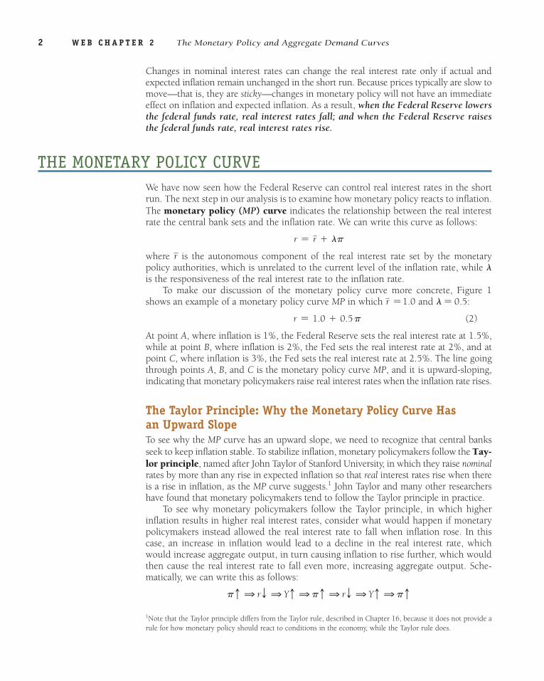
The MoneTAry Policy curveWe have now seen how the Federal Reserve can control real interest rates in the short run. The next step in our analysis is to examine how monetary policy reacts to inflation. The monetary policy (MP) curve indicates the relationship between the real interest rate the central bank sets and the inflation rate. We can write this curve as follows:

r = r + lp

where r is the autonomous component of the real interest rate set by the monetary policy authorities, which is unrelated to the current level of the inflation rate, while l is the responsiveness of the real interest rate to the inflation rate.

To make our discussion of the monetary policy curve more concrete, Figure 1 shows an example of a monetary policy curve MP in which r = 1.0 and l = 0.5:

r = 1.0 + 0.5 p (2)

At point A, where inflation is 1%, the Federal Reserve sets the real interest rate at 1.5%, while at point B, where inflation is 2%, the Fed sets the real interest rate at 2%, and at point C, where inflation is 3%, the Fed sets the real interest rate at 2.5%. The line going through points A, B, and C is the monetary policy curve MP, and it is upward-sloping, indicating that monetary policymakers raise real interest rates when the inflation rate rises.

The Taylor Principle: Why the Monetary Policy Curve Has an Upward SlopeTo see why the MP curve has an upward slope, we need to recognize that central banks seek to keep inflation stable. To stabilize inflation, monetary policymakers follow the Tay-lor principle, named after John Taylor of Stanford University, in which they raise nominal rates by more than any rise in expected inflation so that real interest rates rise when there is a rise in inflation, as the MP curve suggests.1 John Taylor and many other researchers have found that monetary policymakers tend to follow the Taylor principle in practice.

To see why monetary policymakers follow the Taylor principle, in which higher inflation results in higher real interest rates, consider what would happen if monetary policymakers instead allowed the real interest rate to fall when inflation rose. In this case, an increase in inflation would lead to a decline in the real interest rate, which would increase aggregate output, in turn causing inflation to rise further, which would then cause the real interest rate to fall even more, increasing aggregate output. Sche-matically, we can write this as follows:

pc 1 rT 1 Yc 1 pc 1 rT 1 Yc 1 pc

1Note that the Taylor principle differs from the Taylor rule, described in Chapter 16, because it does not provide a rule for how monetary policy should react to conditions in the economy, while the Taylor rule does.



As a result, inflation would continually keep rising and spin out of control. Indeed, this is exactly what happened in the 1970s, when the Federal Reserve did not raise nominal interest rates by as much as inflation rose, so that real interest rates fell. Inflation accel-erated to over 10%.2

Shifts in the MP CurveIn common parlance, the Federal Reserve is said to tighten monetary policy when it raises real interest rates, and to ease it when it lowers real interest rates. It is important, however, to distinguish between changes in monetary policy that shift the monetary policy curve, which we call autonomous changes, and the Taylor principle–driven changes that are reflected as movements along the monetary policy curve, which are called automatic adjustments to interest rates.

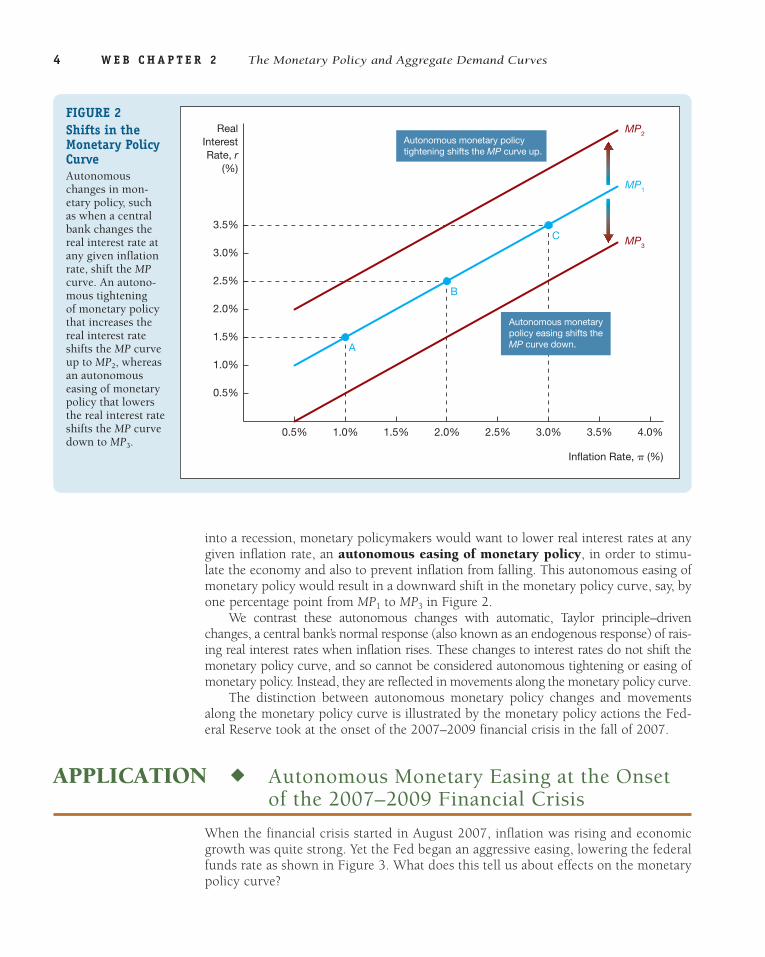
Central banks may make autonomous changes to monetary policy for various rea-sons. They may wish to change the inflation rate from its current value. For example, to lower inflation they could increase r by one percentage point, and so raise the real inter-est rate at any given inflation rate, what we will refer to as an autonomous tightening of monetary policy. This autonomous monetary tightening would shift the monetary policy curve upward by one percentage point from MP1 to MP2 in Figure 2, thereby causing the economy to contract and inflation to fall. Or, the banks may have informa-tion above and beyond what is happening to inflation that suggests interest rates must be adjusted to achieve good economic outcomes. For example, if the economy is going

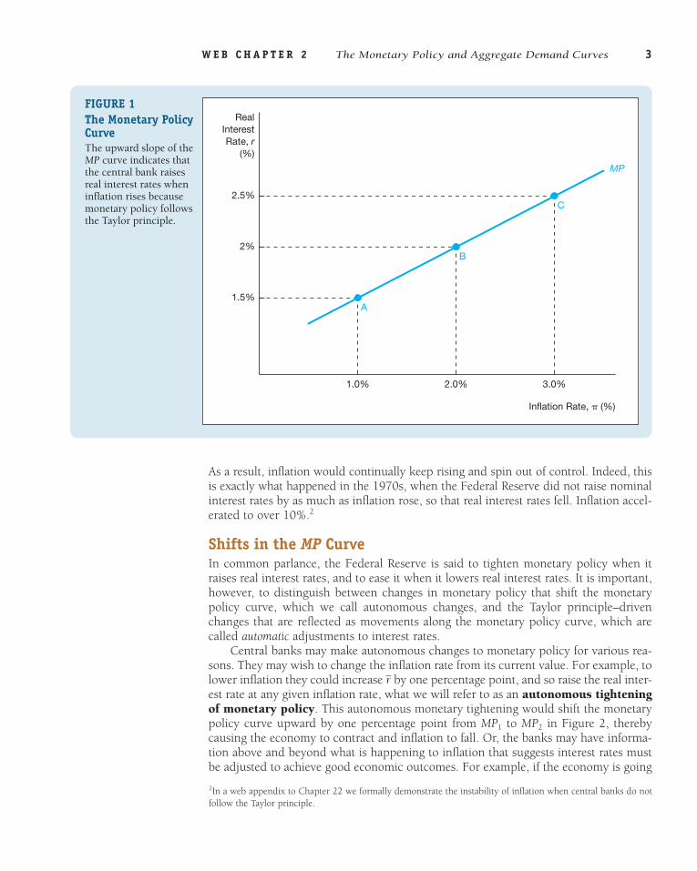
FigURE 1 The Monetary Policy CurveThe upward slope of the MP curve indicates that the central bank raises real interest rates when inflation rises because monetary policy follows the Taylor principle.

Inflation Rate, � (%)

RealInterestRate, r

(%)

1.5%

2%

2.0%1.0%

A

B

C2.5%

3.0%

MP

2In a web appendix to Chapter 22 we formally demonstrate the instability of inflation when central banks do not follow the Taylor principle.



into a recession, monetary policymakers would want to lower real interest rates at any given inflation rate, an autonomous easing of monetary policy, in order to stimu-late the economy and also to prevent inflation from falling. This autonomous easing of monetary policy would result in a downward shift in the monetary policy curve, say, by one percentage point from MP1 to MP3 in Figure 2.

We contrast these autonomous changes with automatic, Taylor principle–driven changes, a central bank’s normal response (also known as an endogenous response) of rais-ing real interest rates when inflation rises. These changes to interest rates do not shift the monetary policy curve, and so cannot be considered autonomous tightening or easing of monetary policy. Instead, they are reflected in movements along the monetary policy curve.

The distinction between autonomous monetary policy changes and movements along the monetary policy curve is illustrated by the monetary policy actions the Fed-eral Reserve took at the onset of the 2007–2009 financial crisis in the fall of 2007.

ApplicATion ◆ Autonomous Monetary Easing at the Onset of the 2007–2009 Financial Crisis

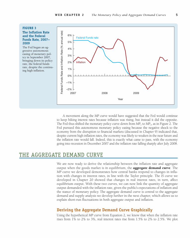
When the financial crisis started in August 2007, inflation was rising and economic growth was quite strong. Yet the Fed began an aggressive easing, lowering the federal funds rate as shown in Figure 3. What does this tell us about effects on the monetary policy curve?


RealInterestRate, r

(%)

1.5%

1.5%

2.0%

2.5%

2.0%1.0% 2.5%

A

B

C

Autonomous monetary policytightening shifts the MP curve up.

Autonomous monetarypolicy easing shifts theMP curve down.

1.0%

0.5%

3.0%

3.5%

0.5% 4.0%3.0%

MP3

MP2

3.5%

MP1

FigURE 2 Shifts in the Monetary Policy CurveAutonomous changes in mon-etary policy, such as when a central bank changes the real interest rate at any given inflation rate, shift the MP curve. An autono-mous tightening of monetary policy that increases the real interest rate shifts the MP curve up to MP2, whereas an autonomous easing of monetary policy that lowers the real interest rate shifts the MP curve down to MP3.



A movement along the MP curve would have suggested that the Fed would continue to keep hiking interest rates because inflation was rising, but instead it did the opposite. The Fed thus shifted the monetary policy curve down from MP1 to MP3, as in Figure 2. The Fed pursued this autonomous monetary policy easing because the negative shock to the economy from the disruption to financial markets (discussed in Chapter 9) indicated that, despite current high inflation rates, the economy was likely to weaken in the near future and the inflation rate would fall. Indeed, this is exactly what came to pass, with the economy going into recession in December 2007 and the inflation rate falling sharply after July 2008.

The AggregATe deMAnd curveWe are now ready to derive the relationship between the inflation rate and aggregate output when the goods market is in equilibrium, the aggregate demand curve. The MP curve we developed demonstrates how central banks respond to changes in infla-tion with changes in interest rates, in line with the Taylor principle. The IS curve we developed in Chapter 20 showed that changes in real interest rates, in turn, affect equilibrium output. With these two curves, we can now link the quantity of aggregate output demanded with the inflation rate, given the public’s expectations of inflation and the stance of monetary policy. The aggregate demand curve is central to the aggregate demand and supply analysis we develop further in the next chapter, which allows us to explain short-run fluctuations in both aggregate output and inflation.

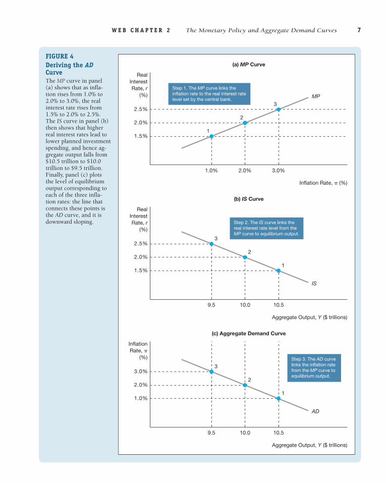
Deriving the Aggregate Demand Curve graphicallyUsing the hypothetical MP curve from Equation 2, we know that when the inflation rate rises from 1% to 2% to 3%, real interest rates rise from 1.5% to 2% to 2.5%. We plot

2%

1%

5%

3%

–1%

–2%

0%

2007 2008 2009

Year

Fed

eral

Fun

ds

Rat

e an

d In

flatio

n R

ate

(% a

nnua

l rat

e)

6%

4%

Inflation

Federal Funds rate

FigURE 3 The inflation Rate and the Federal Funds Rate, 2007–2009The Fed began an ag-gressive autonomous easing of monetary pol-icy in September 2007, bringing down its policy rate, the federal funds rate, despite the continu-ing high inflation.



these points in panel (a) of Figure 4 to create the MP curve. In panel (b), we graph the IS curve described in Equation 13 of Chapter 20 (Y = 12 - r). As the real interest rate rises from 1.5% to 2% to 2.5%, the equilibrium moves from point 1 to point 2 to point 3 and aggregate output falls from $10.5 trillion to $10 trillion to $9.5 trillion. In other words, as real interest rates rise, investment and net exports decline, leading to a reduction in aggregate demand. Panels (a) and (b) demonstrate that as inflation rises from 1% to 2% to 3%, the equilibrium moves from point 1 to point 2 to point 3 in panel (c), and aggregate output falls from $10.5 trillion to $10 trillion to $9.5 trillion.

The line that connects the three points in panel (c) is the aggregate demand curve, AD, and it indicates the level of aggregate output corresponding to each of the three real interest rates consistent with equilibrium in the goods market for any given inflation rate. The aggregate demand curve has a downward slope, because a higher inflation rate leads the central bank to raise real interest rates, thereby lowering planned spending, and hence lowering the level of equilibrium aggregate output.

By using some algebra (see the FYI box, “Deriving the Aggregate Demand Curve Algebraically”), the AD curve in Figure 4 can be written numerically as follows:

Y = 11 - 0.5 p (3)

Factors That Shift the Aggregate Demand CurveMovements along the aggregate demand curve describe how the equilibrium level of aggregate output changes when the inflation rate changes. When factors besides the inflation rate change, however, the aggregate demand curve can shift. We first review the factors that shift the IS curve, and then consider other factors that shift the AD curve.

FYi Deriving the Aggregate Demand curve Algebraically

To derive the numerical AD curve, we start by taking the numerical IS curve, Equation 13, from the previ-ous chapter,

Y = 12 - r

and then substitute in for r from the numerical MP curve in Equation 2, r = 1.0 + 0.5 p, to yield

Y = 12 - (1.0 + 0.5 p) = (12 - 1) - 0.5 p = 11 - 0.5 p

as in the text.Similarly, we can derive a more general version of

the AD curve, using the algebraic version of the IS curve from Equation 12 in Chapter 20:

Y = 3C + I - df + G + N X - mpc * T4

*1

1 - mpc-

d + x

1 - mpc* r

and then substitute for r from the algebraic MP curve in Equation 1, r = r + lp, to yield the more general AD curve:

Y = 3C + I - df + G + N X - mpc * T4*

1

1 - mpc-

d + x

1 - mpc* (r + lp)

(4)



FigURE 4 Deriving the AD CurveThe MP curve in panel (a) shows that as infla-tion rises from 1.0% to 2.0% to 3.0%, the real interest rate rises from 1.5% to 2.0% to 2.5%. The IS curve in panel (b) then shows that higher real interest rates lead to lower planned investment spending, and hence ag-gregate output falls from $10.5 trillion to $10.0 trillion to $9.5 trillion. Finally, panel (c) plots the level of equilibrium output corresponding to each of the three infla-tion rates: the line that connects these points is the AD curve, and it is downward sloping.

Step 1. The MP curve links thein�ation rate to the real interest ratelevel set by the central bank.


RealInterestRate, r

(%)

3.0%

(a) MP Curve

2.0%1.0%

1.5%

2.5%

2.0%

1

2

3MP

(b) IS Curve

Aggregate Output, Y ($ trillions)

RealInterestRate, r

(%)

10.510.09.5

1.5%

2.5%

2.0%

IS

3

2

1

(c) Aggregate Demand Curve


InflationRate, �

(%)

10.510.09.5

1.0%

3.0%

2.0%

AD

3

2

1

Step 2. The IS curve links thereal interest rate level from theMP curve to equilibrium output.

Step 3. The AD curvelinks the in�ation ratefrom the MP curve toequilibrium output.



Shifts in the IS curve We saw in the previous chapter that six factors cause the IS curve to shift. It turns out that the same factors cause the aggregate demand curve to shift as well:

1. Autonomous consumption expenditure 2. Autonomous investment spending 3. Government purchases 4. Taxes 5. Autonomous net exports 6. Financial frictions

We examine how changes in these factors lead to a shift in the aggregate demand curve in Figure 5.

Suppose that inflation is at 2.0% and so the MP curve shows that the real inter-est rate is at 2.0% in Figure 5 panel (a). The IS1 curve in panel (b) then shows that the equilibrium level of output is at $10 trillion at point A1, which corresponds to an equilibrium level of output of $10 trillion at point A1 on the AD1 curve in panel (c). Now suppose there is rise in, for example, government purchases by $1 trillion. Panel (b) shows that with the inflation rate and real interest both held constant at 2.0%, the equilibrium moves from point A1 to point A2, with output rising to $12.5 trillion,3 so the IS curve shifts to the right from IS1 to IS2. The rise in output to $12.5 trillion means that holding inflation and the real interest rate constant, the equilibrium in panel (c) also moves from point A1 to point A2, and so the AD curve also shifts to the right from AD1 to AD2.

Figure 5 shows that any factor that shifts the IS curve shifts the aggregate demand curve in the same direction. Therefore, “animal spirits” that encourage a rise in autonomous consumption expenditure or planned investment spending, a rise in government purchases, an autonomous rise in net exports, a fall in taxes, or a decline in financial frictions—all of which shift the IS curve to the right—will also shift the aggregate demand curve to the right. Conversely, a fall in autonomous consumption expenditure, a fall in planned investment spending, a fall in government purchases, a fall in net exports, a rise in taxes, or a rise in financial frictions will cause the aggregate demand curve to shift to the left.

Shifts in the MP curve We now examine what happens to the aggregate de-mand curve when the MP curve shifts. Suppose that the Federal Reserve decides to autonomously tighten monetary policy by raising the real interest rate by one per-centage point at any given level of the inflation rate because it is worried about the economy overheating. At an inflation rate of 2.0%, the real interest rate rises from 2.0% to 3.0% in Figure 6. The MP curve shifts up from MP1 to MP2 in panel (a). Panel (b) shows that when the inflation rate is at 2.0%, the higher interest rate results in the equilibrium moving from point A1 to A2 on the IS curve, with output falling from $10 trillion to $9 trillion. The lower output of $9 trillion occurs because the higher real interest leads to a decline in investment and net exports, which lowers aggregate demand. The lower output of $9 trillion then decreases the equilibrium output level from point A1 to point A2 in panel (c), and so the AD curve shifts to the left from AD1 to AD2.

3As we saw in the numerical example in Chapter 20, a rise in government purchases by $1 trillion leads to a $2.5 trillion increase in equilibrium output at any given real interest rate, and this is why output rises from $10 trillion to $12.5 trillion when the real interest rate is 2.0%.



Step 1. The MP curve links thein�ation rate to the real interest ratelevel set by the central bank.


RealInterestRate, r

(%)

(a) MP Curve

2.0%

2.0%A

MP

(b) IS Curve


RealInterestRate, r

(%)

12.510.0

IS2

IS1

A2A1

(c) Aggregate Demand Curve


InflationRate, �

(%)

10.0 12.5

AD2

2.0%

AD1

A2A1

Step 2. A rise in government purchasesincreases equilibrium output, shiftingthe IS curve rightward . . .

Step 3. and shifting theAD curve rightward.

2.0%

FigURE 5 Shift in the AD Curve from Shifts in the IS CurveAt a 2% inflation rate in panel (a), the monetary policy curve indicates that the real interest rate is 2%. An increase in government purchases shifts the IS curve to the right in panel (b). At a given inflation rate and real interest rate of 2.0%, equilibrium output rises from $10 trillion to $12.5 trillion, which is shown as a movement from point A1 to point A2 in panel (c), shifting the aggregate demand curve to the right from AD1 to AD2. Any factor that shifts the IS curve shifts the AD curve in the same direction.



Step 1. Autonomous monetary policy tightening increases the real interest rate . . .


RealInterestRate, r

(%)

(a) MP

2.0%

2.0%A1

A2

MP1

MP2

(b) IS


RealInterestRate, r

(%)

10.09.0

IS

A2

A1

(c) Aggregate Demand


InflationRate, �

(%)

10.09.0

2.0%

AD1

AD2

A2 A1

Step 2. causing movementalong the IS curve, decreasingequilibrium output . . .

Step 3. and shiftingthe AD curve leftward.

2.0%

3.0%

3.0%

FigURE 6 Shift in the AD Curve from Autonomous Monetary Policy TighteningAutonomous monetary tightening that raises real interest rates by one percentage point at any given inflation rate shifts the MP curve up from MP1 to MP2 in panel (a). With the inflation rate at 2.0%, the higher 3% interest rate results in a movement from point A1 to A2 on the IS curve, with output falling from $10 trillion to $9 trillion. This change in equilibrium output leads to movement from point A1 to point A2 in panel (c), shifting the aggregate demand curve to the left from AD1 to AD2.



Our conclusion from Figure 6 is that an autonomous tightening of monetary policy—that is, a rise in the real interest rate at any given inflation rate—shifts the aggregate demand curve to the left. Similarly, an autonomous easing of monetary policy shifts the aggregate demand curve to the right.

We have now derived and analyzed the aggregate demand curve—an essential ele-ment in the aggregate demand and supply framework that we examine in the next chapter. We will use the aggregate demand curve in this framework to determine both aggregate output and inflation, as well as to examine events that cause these variables to change.

Summary 1. When the Federal Reserve lowers the federal funds rate

by providing more liquidity to the banking system, real interest rates fall in the short run; and when the Federal Reserve raises the federal funds rate by reducing the liquidity in the banking system, real interest rates rise in the short run.

2. The monetary policy (MP) curve shows the relationship between inflation and the real interest rate arising from monetary authorities’ actions. Monetary policy follows the Taylor principle, in which higher inflation results in higher real interest rates, as represented by a movement up along the monetary policy curve. An autonomous tightening of monetary policy occurs when monetary policymakers raise the real interest rate at any given inflation rate, resulting in an upward shift in the mon-etary policy curve. An autonomous easing of monetary policy and a downward shift in the monetary policy

curve occurs when monetary policymakers lower the real interest rate at any given inflation rate.

3. The aggregate demand curve tells us the level of equilib-rium aggregate output (which equals the total quantity of output demanded) for any given inflation rate. It slopes downward because a higher inflation rate leads the central bank to raise real interest rates, which leads to a lower level of equilibrium output. The aggregate demand curve shifts in the same direction as a shift in the IS curve; hence it shifts to the right when govern-ment purchases increase, taxes decrease, “animal spirits” encourage consumer and business spending, autono-mous net exports increase, or financial frictions decrease. An autonomous tightening of monetary policy—that is, an increase in real interest rates at any given inflation rate—leads to a decline in aggregate demand and the aggregate demand curve shifts to the left.

Key Termsaggregate demand curve, p. 5

autonomous easing of monetary policy, p. 4

autonomous tightening of monetary policy, p. 3

monetary policy (MP) curve, p. 2

Taylor principle, p. 2

QuestionsAll questions are available in MyEconLab at www.myeconlab.com.

1. When the inflation rate increases, what happens to the fed funds rate? Operationally, how does the Fed adjust the fed funds rate?

2. What is the key assumption underlying the Fed’s ability to control the real interest rate?

3. Why is it necessary for the MP curve to have an upward slope?

4. If l = 0, what does that imply about the relationship between the nominal interest rate and the inflation rate?

5. How does an autonomous tightening or easing of monetary policy by the Fed affect the MP curve?

6. How is an autonomous tightening or easing of mon-etary policy different from a change in the real interest rate due to a change in the current inflation rate?

7. Suppose that a new Fed chair is appointed, and his or her approach to monetary policy can be summarized by



the following statement: “I care only about increasing employment; inflation has been at very low levels for quite some time; my priority is to ease monetary policy to promote employment.” How would you expect the monetary policy curve to be affected, if at all?

8. “The Fed decreased the fed funds rate in late 2007, even though inflation was increasing. This demon-strates a violation of the Taylor principle.” Is this state-ment true, false, or uncertain? Explain your answer.

9. What factors affect the slope of the aggregate demand curve?

10. “Autonomous monetary policy is more effective at changing output when l is higher” Is this statement true, false, or uncertain? Explain your answer.

11. If net exports were not sensitive to changes in the real interest rate, would monetary policy be more—or less—effective in changing output?

12. How does an autonomous tightening or easing of mone-tary policy by the Fed affect the aggregate demand curve?

13. For each of the following, describe how (if at all), the IS curve, MP curve, and AD curves are affected.

a. A decrease in financial frictions.

b. An increase in taxes, and an autonomous easing of monetary policy.

c. An increase in the current inflation rate.

d. A decrease in autonomous consumption.

e. Firms become more optimistic about the future of the economy.

f. The new Federal Reserve chair begins to care more about fighting inflation.

14. What would be the effect of an increase in U.S. net exports on the aggregate demand curve? Would an increase in net exports affect the monetary policy curve? Explain why or why not.

15. Why does the aggregate demand curve shift when “animal spirits” change?

16. If government spending increases while taxes are raised to keep the budget balanced, what happens to the aggregate demand curve?

17. Suppose that government spending is increased at the same time that an autonomous monetary policy tight-ening occurs. What will happen to the position of the aggregate demand curve?

18. “If f increases, then the Fed can keep output con-stant by reducing the real interest rate by the same amount as the increase in financial frictions.” Is this statement true, false, or uncertain? Explain your answer.

All applied problems are available in MyEconLab at www.myeconlab.com.

19. Assume the monetary policy curve is given by r = 1.5 + 0.75p.

a. Calculate the real interest rate when the inflation rate is 2%, 3%, and 4%.

b. Draw the graph of the MP curve, labeling the points from part (a).

c. Assume now that the monetary policy curve is r = 2.5 + 0.75p. Does the new monetary policy curve represent an autonomous tightening or loosening of monetary policy?

d. Calculate the real interest rate when the inflation rate is 2%, 3%, and 4%, and draw the new MP curve showing the shift frompart (b).

20. Use an IS curve and an MP curve to derive graphically the AD curve.

21. Suppose the monetary policy curve is given by r = 1.5 + 0.75p, and the IS curve is Y = 13 – r.

a. Calculate an expression for the aggregate demand curve.

b. Calculate the real interest rate and aggregate output when the inflation rate is 2%, 3%, and 4%.

c. Draw graphs of the IS, MP, and AD curves, labeling the points in the appropriate graphs from part (b) above.

22. Consider an economy described by the following:

C = 4 trillion I = 1.5 trillion

G = 3.0 trillion T = 3.0 trillion

N X = 1.0 trillion f = 0

mpc = 0.8 d = 0.35 x = 0.15 l = 0.5 r = 2

Applied Problems



a. Derive expressions for the MP curve and AD curve.

b. Calculate the real interest rate and aggregate output when π 5 2 and π 5 4.

c. Draw a graph of the MP curve and AD curve, indicating the points in part (b) above.

23. Consider an economy described by the following:

C = 3.25 trillion I = 1.3 trillion

G = 3.5 trillion T = 3.0 trillion

N X = -1.0 trillion f = 1

mpc = 0.75 d = 0.3 x = 0.1 l = 1 r = 1

a. D erive expressions for the MP curve and AD curve.

b. Assume that π = 1. What is the real interest rate, equilibrium level of output, consumption, planned investment, and net exports?

c. Suppose the Fed increases r to r = 2. Calculate what happens to the real interest rate, equilibrium level of output, consumption, planned investment, and net exports.

d. Considering that output, consumption, planned investment, and net exports all decreased in part (c), why might the Fed choose to increase r ?

24. Consider the economy described in Applied Problem 23.

a. Derive expressions for the MP curve and AD curve.

b. Assume that π 5 2. What is the real interest rate and equilibrium level of output?

c. Suppose government spending increases to $4 trillion. What happens to equilibrium output?

d. If the Fed wanted to keep output constant, then what monetary policy change should occur?

25. Suppose the MP curve is given as r 5 2 1 π, and the IS curve is given as Y 5 20 2 2r.

a. Derive an expression for the AD curve, and draw a graph labeling points at π 5 0, π 5 4, and π 5 8.

b. Suppose that l increases to l = 2. Derive an expression for the new AD curve, and draw the new AD curve using the graph from part (a).

c. What does your answer to part (b) say about the relationship between a central bank’s distaste for inflation and the slope of the AD curve?

Web Exercises 1. Go to http://www.federalreserve.gov/pf/pdf/pf_2.pdf.

Review what the Fed says its goals are for monetary policy. Explain why these are consistent with the Taylor principle.

2. Go to www.federalreserve.gov/fomc/. Read the latest FOMC statement and the minutes of the most recent

FOMC meeting. Are the statement and the discussion in the minutes consistent with the Taylor principle. Review what the Fed says its goals are for monetary policy. Explain why these are consistent with the Taylor principle.

Web Referenceshttp://www.federalreserve.gov/pf/pf.htm

Describes the purposes and functions of the Federal Reserve System and its rationale for the conduct of monetary policy.

www.federalreserve.gov/fomc

Provides information on all the FOMC’s actions, including the statement and minutes for each meeting.


WEB CHAPTER 2 WEB CHAPT 1 2 ER -...

Documents

Transcript of WEB CHAPTER 2 WEB CHAPT 1 2 ER -...