Wealth, Health, and Child Development: Evidence fromAdministrative Data on Swedish Lottery Players∗

David Cesarini† Erik Lindqvist‡ Robert Östling§ Björn Wallace¶

March 10, 2015

Abstract

We use administrative data on Swedish lottery players to estimate the causal impact ofwealth on players’own health and their children’s health and developmental outcomes. Ourestimation sample is large, virtually free of attrition, and allows us to control for the factors —such as the number of lottery tickets —conditional on which the prizes were randomly assigned.In adults, we find no evidence that wealth impacts mortality or health care utilization, withthe possible exception of a small reduction in the consumption of mental health drugs. Ourestimates allow us to rule out effects on 10-year mortality one sixth as large the cross-sectionalgradient. In our intergenerational analyses, we find that wealth increases children’s health careutilization in the years following the lottery and may also reduce obesity risk. The effectson most other child outcomes, which include drug consumption, scholastic performance, andskills, can usually be bounded to a tight interval around zero. Overall, our findings suggestthat correlations observed in affl uent, developed countries between (i) wealth and health or (ii)parental income and children’s outcomes do not reflect a causal effect of wealth.

Keywords: Health; Mortality; Health care; Child health; Child development; Human capital;Wealth; Income; Lotteries.

JEL codes: D91, I10, I12, I14, J13, J24.

∗We thank seminar audiences at various places for helpful comments. We are also grateful to Dan Benjamin,Dalton Conley, Tom Cunningham, George Davey Smith, Oskar Erixon, Jonathan Gruber, Jennifer Jennings, SandyJencks, Magnus Johannesson, David Laibson, Rita Ginja, Matthew Notowidigdo, Per Petterson-Lidbom, JohanReutfors, Bruce Sacerdote, and Jonas Vlachos for stimulating comments and conversations that helped us improvethe paper, and to Richard Foltyn, Renjie Jiang, Krisztian Kovacs, Odd Lyssarides, Jeremy Roth, and Erik Tengbjörkfor research assistance. We are indebted to Kombilotteriet and Svenska Spel for very generously providing us withtheir data. This paper is part of a project hosted by the Research Institute of Industrial Economics (IFN). We aregrateful to IFN Director Magnus Henrekson for his strong commitment to the project and to Marta Benkestock forsuperb administrative assistance. The project is financially supported by two large grants from the Swedish ResearchCouncil (VR) and Handelsbanken’s Research Foundations. We also gratefully acknowledge financial support fromthe Russell Sage Foundation, the US National Science Foundation and the Swedish Council for Working Life, andSocial Research (FAS). We take responsibility for any remaining mistakes.†Center for Experimental Social Science, Department of Economics, New York University, USA, Division of Social

Science, New York University Abu Dhabi, Abu Dhabi, United Arab Emirates and Research Institute of IndustrialEconomics (IFN), Stockholm, Sweden. E-mail: david.cesarini@nyu.edu.‡Department of Economics, Stockholm School of Economics and Research Institute of Industrial Economics (IFN),

Stockholm, Sweden. E-mail: erik.lindqvist@hhs.se.§Robert Östling, Institute for International Economic Studies, Stockholm University, Stockholm, Sweden. E-mail:

robert.ostling@iies.su.se.¶Björn Wallace, University of Cambridge, Cambridge, United Kingdom. E-mail: bfnw2@cam.ac.uk.

1 Introduction

At every stage in the life cycle, health is robustly associated with various markers for socioeconomic

status (SES) such as income, educational attainment, or occupational prestige (Currie 2009, Cutler,

Lleras-Muney, and Vogl 2011, Smith 1999). These relationships manifest themselves early. For

example, children from low-income households weigh less at birth, are more likely to be born

prematurely, and are increasingly at greater risk for chronic health conditions as they age (Brooks-

Gunn and Duncan 1997, Currie 2009, Newacheck and Halfon 1998). Childhood health is in turn

positively related to a number of later outcomes, including skills, scholastic achievement, and

adult economic status (Currie 2009, Smith 2009). In adults, it is also a well-established fact

that individuals with higher incomes enjoy better health outcomes (Deaton 2002, Smith 1999).

Descriptive research has uncovered these positive relationships in many different countries and

time periods, and in many different subpopulations (Cutler, Lleras-Muney, and Vogl 2011, Deaton

2002, Smith 1999).

Although the existence of these gradients for adult health and child outcomes is not contro-

versial, credibly elucidating their underlying causal pathways has proven challenging, as concerns

about reverse causation and omitted variable bias often loom large (Baker and Stabile 2011, Currie

2009, Cutler, Lleras-Muney, and Vogl 2011, Chandra and Vogl 2010, Deaton 2002). One review

article on the causes and consequences of early childhood health notes that “the number of stud-

ies associating poor child outcomes with low SES far exceeds the number that make substantive

progress on this diffi cult question of causality” (Baker and Stabile 2011, p. 8). Writing about

the adult health gradient, Deaton (2002) concludes that “[t]here is no general agreement about

[its] causes ... [A]nd what apparent agreement there is is sometimes better supported by repeated

assertion than by solid evidence”(p. 15).

In this paper, we use the randomized assignment of lottery prizes in three samples of Swedish

lottery players to estimate the causal effect of wealth on players’health and their children’s health

and development. Though the prizes vary in magnitude, most of our identifying variation comes

from prizes that are large even relative to a typical Swede’s lifetime income. The estimates we

report are therefore useful for testing and refining hypotheses about the sources of the relationship

between permanent income and health outcomes.

Our study has three key methodological features that enable us to make stronger inferences

about the causal impact of wealth than previous lottery studies evaluating the effect of wealth on

health (Apouey and Clark 2014, Gardner and Oswald 2007, van Kippersluis and Galama 2013,

Lindahl 2005). First, we observe the factors conditional on which the lottery wealth is randomly

assigned, allowing us to leverage only the portion of lottery-induced variation in wealth that is

exogenous. Second, the size of the prize pool is almost one billion dollars — two orders of mag-

nitude larger than in any previous study of lottery players’health. Third, Sweden’s high-quality

administrative data allow us to observe a rich set of outcomes, some of which are realized over 20

years after the event, in a virtually attrition-free sample.

Our data also allow us to address many (but not all) concerns about the external validity of

2

studies of lottery players. The lotteries we study were popular across broad strata of Swedish society,

and players are hence fairly representative in terms of demographic and health characteristics.

Another frequently voiced concern is that lottery wealth is different from other types of wealth,

perhaps because people are more cavalier in how they spend lottery wealth or because lottery prizes

are paid in lump sums (whereas many policy changes involve changes to monthly income flows).

One of three lottery samples we study consists of two different sub-lotteries, one of which pays the

prizes in monthly installments rather than lump sums. We find that both wealth shocks seem to

result in sustained consumption increases, and generate similar labor-supply responses that match

the predictions of a standard life cycle model. Overall, we find little evidence that winners squander

their wealth.

We report results from two primary sets of analyses. In our adult analyses, we estimate the

effect of wealth on players’own mortality and health care utilization (hospitalizations and drug

prescriptions). We include several of our health outcomes because of their known relationships

to health behaviors and stress, the two primary mechanisms through which epidemiologists have

proposed that low income can adversely impact cardiovascular health, mental health and the risk

of autoimmune disease (Adler and Newman 2002, Brunner 1997, Marmot and Wilkinson 2009,

Stansfeld, Fuhrer, Shipley, and Marmot 2002, Williams 1990). In our intergenerational analyses,

we study how wealth impacts a number of infant and child health characteristics that have featured

in earlier work (Currie 2009, Baker and Stabile 2011). Given the known associations between early

health and subsequent psychological development, we also examine children’s scholastic achievement

and cognitive and non-cognitive skills. And to explore mechanisms, we ask if there is evidence that

parental behavior adjusts as predicted by standard psychological (Bradley and Corwyn 2002) and

economic (Becker and Tomes 1976) theories of child development.

In our adult analyses, we find that the effect of wealth on mortality and health care utilization

can be bounded to a tight interval around zero. For example, our estimates allow us to rule

out a causal effect of wealth on 10-year adult mortality one sixth as large as the cross-sectional

gradient between mortality and wealth. We continue to find effects that can be bounded away

from the gradient when we stratify the sample by age, income, sex, health, and education. In

our intergenerational analyses, the estimated effect of wealth on child drug consumption, scholastic

performance, and cognitive and non-cognitive skills is always precise enough to bound the parameter

to a tight interval around zero. To illustrate the precision of our intergenerational estimates, the

95% confidence interval of 1M SEK (150,000 USD) net of taxes on ninth-grade GPA range from -

0.08 to 0.03 standard deviation (SD) units. Overall, we estimate precise zero effects when we restrict

the sample to low-income households, to households where the mother won, or to households with

children who were young at the time of the lottery.

We find a few possible exceptions to the overall pattern of null results. In the adult analyses, we

find suggestive evidence that positive wealth shocks lead to a small reduction in the consumption

of mental health drugs. In the intergenerational analyses, we find that lottery wealth increases

the likelihood that players’ children are hospitalized in the years following the lottery, but also

3

that lottery wealth may decrease obesity risk. Yet taken in their entirety, the findings of this paper

suggest that the correlations observed in affl uent, developed countries between (i) wealth and health

or (ii) parental income and children’s outcomes do not reflect a causal effect of wealth. Our paper

thus reinforces skepticism from other quasi-experimental work about giving causal interpretations

to the gradients observed in adults.1

The paper is structured as follows. Section 2 briefly reviews the register data and describes

our pooled lottery data. Section 3 describes our identification strategy, provides evidence of the

(conditional) random assignment of wealth in our data, and discusses the appropriateness of gen-

eralizing from our Swedish sample of lottery players to the Swedish population. In sections 4 and

5, we report the results from the adult and intergenerational analyses. Section 6 concludes with a

discussion that places our findings in the context of the wider literature, and addresses the impor-

tant question of whether our results can be generalized to other developed countries with different

educational and health care systems. Throughout the manuscript, referenced tables and figures

whose names are prefaced by the letter “A”are available in the Online Appendix.

2 Data

To set the stage, Table 1 gives a summary overview of the registers from which we derive our main

outcome variables in the adult and the intergenerational analyses. It also defines three sets of

characteristics —birth, demographic, and health characteristics —that will play a key role in many

of our analyses. The birth characteristics are a third-order age polynomial, an indicator for female,

and an indicator for being born in a Nordic country. The demographic characteristics are income,

and indicator variables for college completion, marital status and retirement status. Finally, the

health controls are (a proxy for) the Charlson co-morbidity index (Charlson, Pompei, Ales, and

MacKenzie 1987) and indicator variables for having been hospitalized in the past five years (i) at

all, (ii) for more than one week, (iii) for circulatory disease, (iv) for respiratory disease, or (v) for

cancer.2

Throughout the paper, we refer to all these characteristics collectively as our set of “baseline”

controls.

[TABLE 1 HERE]

Our analyses are based on a pooled sample of lottery players who, along with their children, were

merged to administrative records, using information about players personal identification numbers

1 For evidence on wealth and adult health, see Adams, Hurd, McFadden, Merrill, and Ribeiro (2003), Adda, Banks,and von Gaudecker (2009), Frijters, Haisken-DeNew, and Shields (2005), Meer, Miller, and Rosen (2003), Snyderand Evans (2006) and Stowasser, Heiss, McFadden, and Winter (2011). Quasi-experimental evidence on the effect ofhousehold income on child outcomes is scarcer and the results are more mixed, but see, e.g., Akee, Copeland, Keeler,Angold, and Costello (2010), Dahl and Lochner (2012), Duncan, Morris, and Rodrigues (2011), Milligan and Stabile(2011), Salkind and Haskins (1982) and Sacerdote (2007).

2 For details on the Charlson index, see Online Appendix section 6.5.

4

(PINs).3 Our basic identification strategy is to use the data and knowledge about the institutional

details of each of the three lotteries that comprise the pooled sample to define cells within which

lottery prizes are randomly assigned. In our analyses, we then control for the cell fixed effects

in regressions of health and child outcomes on the size of the lottery prize won. Because the

construction of the cells varies by lottery, we discuss each separately. For expositional clarity, we

begin by describing the construction of the cells used in the adult analyses; the construction of the

intergenerational cells is a straightforward extension described in section 3.

2.1 Prize-linked Savings (PLS) Accounts

Prize-linked savings accounts (PLS) are savings accounts that incorporate a lottery element instead

of paying interest (Kearney, Tufano, Guryan, and Hurst 2010). PLS accounts have existed in Sweden

since the late 1940s and were originally subsidized by the government. The subsidies ceased in 1985,

at which point the government authorized banks to offer prize-linked-savings products under new

names. Two systems were put into place. The savings banks (Sparbankerna) started offering their

clients a PLS-product known as the Million Account (“Miljonkontot”), whereas the remaining banks

joined forces and offered a PLS product known as the Winner Accounts (“Vinnarkontot”). Each

system had over 2 million accounts, implying that one in two Swedes held a PLS account.

Our analyses are based on two sources of information about the Winner Account system that

were retrieved from the National Archives: a set of microfiche images with account data and prize

lists printed on paper (see PLS Figures 2-3 in the Online Appendix). One separate microfiche

volume exists for each monthly PLS draw that took place between December 1986 and December

1994 (the “fiche period”). Each volume contains one row of data for each account in existence at

the time, with information about the account number, the account owner’s PIN, and the number of

tickets purchased. The prize lists, which are available for each draw until 2003, contain information

about the account numbers of all winning accounts and the prizes won (type of prize and prize

amount). The prize lists do not contain the account owner’s PIN, so the fiches are needed to identify

the unique mapping from account number to PIN. After the fiche period, we can identify the PIN

of winners as long as the winning account was active during the fiche period.

Two research assistants working independently manually entered each prize list. We relied on

Optical Character Recognition (OCR) technology to digitize the micro-fiche cards, which contain

almost 200 million rows of data. We also supplemented the OCR-digitized data with manually

gathered data for all accounts that won SEK 100,000 or more during the fiche period. In the

Online Appendix, we provide a detailed account of how we processed the digitized data to construct

a monthly panel for the years 1986 to 1994 with information about accounts, their balance, and

the PIN of the account holder. Our quality checks, which rely in part on the manually collected

data, showed that our algorithm was very effective at correctly mapping prize-winning accounts to

a PIN and determining their account balances (see the Online Appendix).

3 A detailed account of the institutional features of our three lottery samples and the processing of our primary sourcesof lottery data is provided in the Online Appendix (sections 3-5).

5

PLS players could win two types of PLS prizes: fixed prizes and odds prizes. To select the

winners, each account was first assigned one uniquely integer-valued lottery ticket per 100 SEK in

balance. Each prize was then awarded by randomly drawing a winning ticket. Fixed prizes varied

between 1,000 and 2 million SEK net of taxes and (conditional on winning) did not depend on the

account balance. The odds prizes were prizes that instead paid a multiple of 1, 10, or 100 of the

account balance to the winner, with the prize amount capped at 1 million SEK. Conditional on

winning an odds prize, an account with a larger balance hence won a larger prize (except when the

cap was binding).

To construct the cells used in our adult analyses, we use different approaches depending on

the type of prize won. For fixed-prize winners, our identification strategy exploits the fact that

in the population of players who won exactly n fixed prizes in a particular draw, the total sum

of fixed prizes won is independent of the account balance (see Online Appendix Section 3.9 for a

formal treatment). For each draw, we therefore assign winners to the same cell if they won an

identical number of fixed prizes in that draw and define the treatment variable as the sum of fixed

prizes won. This strategy is similar to that used by Imbens, Rubin, and Sacerdote (2001), Hankins,

Hoestra, and Skiba (2011), and Hankins and Hoestra (2011). Because the strategy does not require

information about the number of tickets owned, we can use it for fixed prizes won both during and

after the fiche period.4

To construct odds-prize cells, we match individuals who won exactly one odds-prize to accounts

that won exactly one prize (odds or fixed) in the same draw. For a match to be successful, we

require the accounts to have nearly identical account balances.5 The matching ensures that we are

comparing odds-prize winners with controls who faced the same distribution of possible treatments

before the lottery. A fixed-prize winner who is successfully matched to an odds-prize winner is

moved from the original fixed-prize cell to the cell of the odds-prize winner.6 After the fiche period,

we do not observe account balances and we therefore restrict attention to odds prizes won during

the fiche period (1986-1994).

As we explain in greater detail in the Online Appendix, our final sample is restricted to prize-

winning accounts only, because we find some indications that in the full panel, non-winning accounts

4 We also have prize-list data that predates the fiche period, but we drop these prizes because we are only able toidentify the PINs of individuals who kept their accounts until the beginning of the fiche period. Prize amount mayinteract with unobserved characteristics in determining the likelihood that an account that wins a prize in the pre-ficheperiod is closed down before the start of the fiche period. Such interactions could introduce unobservable differencesbetween large and small winners in the selected sample of accounts whose owners can be identified, invalidating theexperimental comparison.

5 To perform the matching, we discretized the imputed balance variable in increments of 1 for account balances between8 and 10, in increments of 2 for account balances between 10 and 200, increments of 5 for balances between 200 and400 tickets, and intervals of 50 for account balances exceeding 400 tickets. We then performed exact matching on acategorical variable that takes on a unique value for each possible discretized account balance. The coarse bucketsused for accounts with very high balances are of little practical consequence, because the 432 odds-prize-winningaccounts with more than 400 tickets constitute only 4.37% of the treatment variation.

6 We note that the strategy we deploy for the fixed prizes would not work for the odds prizes, because even if wecompared winners of a single odds prize, the prize variation within winners would depend on account balance, whichin turn could be correlated with unobserved determinants of health.

6

in a given draw are not missing at random.7 For the prize-winning accounts, we were able to reliably

match 98.7% of the winning accounts from the fiche period to a PIN, implying a negligibly small

rate of attrition. In practice, little variation in lottery prizes is lost by comparing winners of large

prizes to winners of small prizes (typically 1,000 SEK in the PLS data) instead of comparing winners

of large prizes to non-winners (as we do in Kombi). Because the majority of PLS prizes are small,

the small-prize winners can still be used to accurately estimate the counterfactual trajectories of

large winners.

2.2 The Kombi Lottery

Kombi is a monthly subscription ticket lottery whose proceeds are given to the Swedish Social

Democratic Party and its youth movement. Participants are therefore unrepresentative of the

Swedish population in terms of political ideology. Subscribers are billed monthly for their tickets,

usually by direct debit. Ticket owners automatically participate in regular prize draws in which

they can win cash prizes or merchandise.

Kombilotteriet provided us with an electronic data set with information about the monthly

ticket balance of all Kombi participants since January 1998.8 They also provided us with a list of

all individuals who won 1 million SEK (net of taxes) or more, along with information about the

month and year of the win.9 Our empirical strategy is to compare each winner of a large prize with

“matched controls”who did not win a large prize but owned an identical number of tickets at the

time of the draw. We matched each winner of a large prize to (up to) 100 matched controls who

did not win a large prize in the month of the draw but owned an identical number of tickets and

were similar in terms of age and sex.10 In those cases in which we had fewer than 100, we included

all of them. Our final estimation sample includes the winners of 462 large prizes matched to 46,024

controls (comprising 40,366 unique individuals).

2.3 The Triss Lottery

Triss is a scratch-ticket lottery run since 1986 by Svenska Spel, the Swedish government-owned

gambling operator. Triss lottery tickets can be bought in virtually any Swedish store. Our sample

7 The non-random missingness, which is only statistically detectable because of our very large sample, is due to toidiosyncratic differences in the quality of the microfiche cards over time. Our OCR algorithm assumes that an accountwas opened the first time the software detects the account number in a fiche volume. As a result, the probabilitythat a non-winning account is missing from our panel in a given draw is slightly higher if the account was recentlyopened and close to zero for accounts that have been in existence for several draws. However, the algorithm we useto process the data also incorporates the fact that if an account won in a given draw, it must have existed at thatpoint in time. Because the prize lists are entered manually, we thus observe all winning accounts from a given draw(including winning accounts that were very recently opened).

8 Approximately 1% of the participants are excluded from the panel because they did not provide a valid PIN uponenrollment. However, whether an individual’s PIN is available is determined when a player signs up for the lottery.Individuals with missing PINs are therefore missing for reasons unrelated to the outcome of the lottery.

9 Because the expected value of the cash and merchandize prizes not included in our data is at most a few hundredSEK, ignoring these prizes does not bias our estimates in any quantitatively meaningful way.

10We match on sex and age in order to reduce the amount of noise due to random differences in the characteristics ofwinners and non-winners. The exact matching procedure is described in the Online Appendix.

7

contains winners of two types of Triss prizes: Triss-Lumpsum and Triss-Monthly.

Winners of the Triss-Lumpsum and Triss-Monthly prize are eligible to participate in a morning

TV show broadcast on national television (“TV4 Morgon”). At the show, Triss-Lumpsum winners

draw a prize from a stack of tickets. This stack of tickets is determined by a prize plan that is

subject to occasional revisions. Triss-Lumpsum prizes vary in size from 50,000 to 5 million SEK

(net of taxes). Triss-Monthly winners participate in the same TV show, but draw one ticket that

determines the size of a monthly installment and a second that determines its duration. The tickets

are drawn independently. The durations range from 10 to 50 years, and the monthly installments

range from 10,000 to 50,000 SEK. To make the monthly installments in Triss-Monthly comparable

to the lump-sum prizes in the other lotteries, we convert them to present value using a 2% annual

discount rate.

Svenska Spel provided us a spreadsheet with information on all participants in Triss-Lumpsum

and Triss-Monthly prize draws in the period between 1994 and 2010. The Triss-Monthly prize

was not introduced until 1997. Around 25 Triss-Lumpsum prizes and five Triss-Monthly prizes are

awarded each month. With the help of Statistics Sweden, we were able to use the information in

the spreadsheet (name, age, region of residence, and often also the names of close relatives), to

reliably identify the PINs of 98.7% of the winners of Triss prizes. In the Online Appendix, we

provide a detailed account of the processing of the data and report the results from several quality

controls. The spreadsheet also notes instances in which the participant shared ownership of the

ticket. Our analyses below are based exclusively on the 90% of winners who did not indicate prior

to the TV show that they shared ownership of the lottery tickets. However, all of our main results

are substantively identical with shared prizes included.

Our empirical strategy makes use of the fact that, conditional on making it to the show, prizes

are drawn randomly conditional on the prize plan. We assign players to the same cell if they won

the same type of lottery prize (Triss-Lumpsum or Triss-Monthly) under the same prize plan and

in the same year.

3 Identification Strategy

In our adult analyses, each observation corresponds to a prize won by a player aged 18 or above at

the time of the lottery. Normalizing the year of the lottery to t = 0, our main estimating equation

is given by,

Yi,t = αtPi,0 +Xiβt + Zi,−1γt + εi,t, (1)

where Yi,t is the (possible time-varying) post-lottery outcome of interest, Xi is a vector of cell

fixed effects, and Pi,0 is the prize amount won in million SEK using the price level of 2010. The

key identifying assumption is that Pi,0 is independent of potential outcomes conditional on Xi.

We include the vector of baseline characteristics (defined in Table 1) measured the year before

the lottery, Zi,−1, in order to improve the precision of our estimates. Unless otherwise noted, we

estimate equation (1) using ordinary least squares (OLS).

8

Our intergenerational analyses are based on a version of equation (1) in which the unit of

analysis is the child of a player. In these analyses, we make a distinction between pre- and post-

lottery children. Players’ children who were conceived but not yet aged 18 at the time of the

lottery are defined as pre-lottery children. We refer to children conceived after the lottery as post-

lottery children. If the impact of wealth on fertility is heterogeneous, then this could invalidate

any experimental comparisons of the post-lottery children of winners who won small prizes to post-

lottery of winners who won large prizes. Though wealth effects on the composition of births are

interesting, we restrict the estimation sample to pre-lottery children except when studying infant

health outcomes (which by definition are realized before the lottery in virtually all pre-lottery

children). We discuss and evaluate possible selection effects in the infant health analyses in section

3.2 below.

The cells used in all of our intergenerational analyses are generated following a procedure anal-

ogous to that used for the adult sample, with two important exceptions. First, when generating the

cells, we condition on the lottery playing parent’s number of pre-lottery children, thus ensuring that

the amount won per child is the same within a cell regardless of whether Pi,0 is defined as the prize

won by the winning parent or the prize won per pre-lottery child. In our primary specification, Pi,0is defined as in the adult analyses, but we also report a robustness check with wealth scaled per

child.11 The second difference is that we drop all odds-prize cells in the intergenerational analy-

ses.12 In the intergenerational analyses, we control for the child’s parent’s baseline characteristics

(except retirement status, which does not vary in any meaningful way) and for the child’s birth

characteristics.

Table 2 summarizes our identification strategy in the adult and intergenerational analyses.

[TABLE 2 HERE]

3.1 Inference

We took a number of steps to ensure the standard errors we report convey the precision of our

estimates as accurately as possible. Throughout the paper, we adjust the analytical standard

errors for two sources of non-independence. First, players who win more than one prize will typically

appear more than once in the sample (as will children of players who won multiple times). Second,

in the intergenerational analyses, siblings’ outcomes are clearly not independent. We therefore

reported clustered standard errors (Liang and Zeger 1986) throughout the manuscript. We cluster

at the level of the player in our adult analyses and at the household level in the intergenerational

analyses (using an iterative process that always assigns half-siblings to the same cluster).

The analytical standard errors rely on an asymptotic approximation that may introduce sub-

stantial biases in finite samples. Though our sample size is large, some of the variables are heavily

11 For infant health, we divide the prize sum by the total number of pre- and post-lottery children. For remainingoutcomes, we scale the prize by the number of pre-lottery children.

12 Because the odds-prizes are randomly assigned conditional on account balances, partitioning the odds-prize cells bythe number of pre-lottery children would leave little useful identifying variation.

9

skewed, so standard rules of thumb about the appropriate sample sizes may not apply. To quantify

the amount of finite sample bias, we conducted Monte Carlo simulations in our adult and intergen-

erational estimation samples. In the simulations, we exploit the fact that the prizes are randomly

assigned within cells to obtain the approximate finite-sample distribution of our test statistics un-

der the null hypothesis that the effect of wealth is zero. Procedurally, we generated 1,000 data sets

in which the prizes won by the players (and hence also their children) were permuted within each

cell. For each outcome and each permuted sample, we then estimated equation (1).

In the simulated data, prize amount is (conditionally) independent of the outcome by construc-

tion, so if the p-values obtained from analytical standard errors follow a uniform distribution, we

interpret this finding as evidence that they are reliable. By this criterion, the analytical standard

errors we report in our main analyses are generally reliable. In all our major analyses, we nev-

ertheless supplement analytical standard errors with resampling-based p-values (constructed from

the resampling distribution generated in the Monte Carlo simulations). In some analyses of either

skewed variables (such as prescription drug consumption) or rare binary variables (such as short-run

cause-specific hospitalizations), we occasionally observe non-trivial differences between the analyt-

ical and resampling-based p-values. In such cases, we rely on the resampling-based p-values, which

are usually more conservative.

3.2 Random Assignment

If the identifying assumptions of Table 2 are correct, no covariates determined before the lottery

should have predictive power for the lottery outcome once we condition on the cell fixed effects.

Normalizing the time of the lottery to 0, we test for (conditional) random assignment by running

regressions of the following form:

Pi,0 = Xi,0β + Z−1γ + εi,0, (2)

where Pi,0 is prize money at the time of the event, Xi,0 is the matrix of cell fixed effects, and Z−1 is

the full set of baseline controls (see Table 1) measured at t = −1. To test for random assignment,

in Table 3, we report omnibus p-values for joint significance of the demographic characteristics,

the health characteristics, and their union. We run these randomization tests in the pooled adult

sample, in the four lottery samples, and for parents of pre-lottery children or post-lottery children.

For the pooled sample, we also estimate the equation without cell fixed effects. Overall, the results in

Table 3 are consistent with our null hypothesis that wealth is randomly assigned once we condition

on the cell fixed effects.13

[TABLE 3 HERE]

13 Table A3 shows an alternative test of random assignment where we split each cell by the amount won (below or abovethe cell median). We also tested for systematic attrition by examining if wealth impacts the likelihood that players’move abroad or that their children are missing from key registers (see Table A1).

10

Because the hypothesis of conditional random assignment of wealth is the least credible in the

potentially selected sample of parents with post-lottery children, we also tested whether wealth

shocks have an impact on fertility (a fundamental question in its own right — see Becker and

Tomes (1976)). We found that in players below the age of 50, 1M SEK increases male fertility

by 0.055 children (95% CI 0.014-0.096). We find little evidence of an impact in women. The

endogenous fertility response observed in men suggests that interpreting the coeffi cient estimates

in our infant health analyses as reflecting a mix of a causal parameter and a composition-of-birth

effect is appropriate.

3.3 External Validity

In this section, we address a number of questions about the appropriateness of generalizing from

our Swedish sample of lottery players to the Swedish population.

How Representative Are Players? The lottery players are about 10 years older than the average

Swedish adult (see Figure A1 for age distributions). We therefore compared each lottery sample

to a representative sample reweighted to match the sex- and age composition of the lottery. Table

4 shows that the distribution of demographic and health characteristics in our sample of lottery

players is quite similar to the distribution in the reweighted representative sample. We reach similar

conclusions about representativeness when we examine the parents of pre- and post-lottery children

and the health and developmental characteristics of the players’children (Table A4-A7).

[TABLE 4 HERE]

How Large are the Wealth Shocks? To interpret our results, having a basic sense of the type

and magnitude of prizes that comprise most of our identifying variation is helpful. Table 5 reports

the distribution of prizes for each lottery and the pooled adult and intergenerational samples. All

prizes are deflated by a consumer price index normalized to 1 in 2010. The total prize sum in the

pooled sample is 6,661 million SEK ($931 million). To convey a sense of the magnitudes of the

prizes, the median disposable income of the working-age Swedish population in 1998 (the midpoint

of our sample period) was 153,000 SEK in year-2010 prices.

[TABLE 5 HERE]

Although the overwhelming majority of winners are people who won small amounts in the PLS

lottery, most of our identifying variation comes from large prizes, which are much more evenly

distributed across lotteries. For example, the 358,141 prizes below 10,000 SEK in the PLS adult

sample account for 7% of the total prize pool, and dropping them from the sample reduces the total

amount of prize variation by 10%.14 The estimates we report in the paper therefore assign relatively

little weight to the marginal effects of small lottery prizes, even though small prizes account for a

14We define the total amount of identifying variation as the total sum of squares of prizes, where the prizes are demeanedat the level of the cell. We demean the prizes because all our regressions include cell fixed effects, thus ensuring thatall identifying variation comes from comparisons of individuals within a cell.

11

large fraction of the number of prizes won. Consequently, the lottery-induced variation in wealth is

useful for answering questions about the consequences positive wealth changes that are large even

from a life cycle point of view. The wealth shocks we study are thus comparable in magnitude to

wealth changes induced by major changes to capital income taxes, real estate taxes, labor taxes,

or college subsidies.

Is Lottery Wealth Different? A general concern often voiced about studies of lottery winners is

that people may react differently to lottery wealth than other types of wealth shocks (e.g. changes

in taxes, welfare systems, or asset-price fluctuations). This argument can take many specific forms,

one of them being that lottery prizes are usually paid in lump sums whereas many policy changes

involve changes to income flows. Throughout the paper, we therefore test for heterogeneity by

lottery and by type of prize (monthly installments vs. lump sum). In interpreting these estimates,

recall that the Triss-Monthly prizes supplement monthly incomes by $1,200 to $6,000. Hence, they

do not replicate the features of most income support programs particularly well. Rather, they allow

us to evaluate whether our conclusions about the effects of substantial shocks to permanent income

are robust to the mode of payment. The informativeness of the estimates from the Triss-Monthly

sample also varies across outcomes depending on the effective sample size.

According to a folk wisdom, lottery winners spend lottery wealth more frivolously than other

types of wealth. In a companion paper on labor supply (Cesarini, Lindqvist, Notowidigdo, and

Östling 2015), we show that the earnings response to the lottery wealth shock is immediate, modest

in size, seemingly permanent, and surprisingly similar across the four lotteries. The trajectories of

net wealth are also similar across lotteries, and indicate that winners consume a modest fraction

of the prize in each year following the win (Figure A2).15 The indications are thus that winners of

large prizes in all lotteries enjoy a modest but sustained increase in consumption and leisure for an

extended period of time.

4 Adult Health

We use information from the Cause of Death Register to study both overall mortality and cause-

specific mortalities and information from additional registers to study in-patient hospitalizations

and consumption of prescription drugs. We examine deaths and health care utilization events

classified into two cause categories: common causes and hypotheses-based causes. The common

causes are cancer, respiratory disease, cardiovascular disease, and other. The hypotheses-based

15 The figures showing net wealth trajectories are based on annual data from the Wealth Registry, which includesdetailed information on individuals’ year-end net wealth holdings between 1999 and 2007. The limited time spanprevents us from making reliable inferences about the long-term effect of prizes in Triss (1994-) and Kombi (1998-)on net wealth. The wealth measure does not include cash, cars, or other durables, merchandise, assets transferredto other family members, or money that has been concealed from the tax authority. The purchase of a car (or someother consumer durable) worth 100K will thus typically reduce measured wealth by 100K, even though actual netwealth has only declined by 100K minus the resale value of the car. For all of these above reasons, the estimatedeffect of lottery wealth on year-end wealth at t = 0 (on average 6 months after the lottery) only gives an upper boundon the fraction of the wealth shock that is consumed in the year of the lottery. The trajectory for capital income(Figure A3) corroborates the results for net wealth.

12

causes, which we sought to harmonize across registers, include diabetes, ischemic heart disease,

hypertension, cerebrovascular disease, alcohol consumption, injury, and smoking.16

We chose these categories to test some of the hypotheses about the causal pathways from income

to health that have been proposed in economics and epidemiology. Epidemiologists argue that the

stress induced by low income has deleterious health effects, either through relatively proximal

biological mechanisms that divert resources away from the maintenance of long-term health (the

“fight or flight”response) or through behavioral responses such as smoking, excessive drinking, or

unhealthy dieting (Adler and Newman 2002, Williams 1990). These biological mechanisms, in turn,

increase the risk of bad health in the categories covered by our hypotheses-based classification. In

the framework that economists use to study the wealth-health relationship (Grossman 1972), health

is a stock whose malleability may vary over the life cycle (Cutler, Lleras-Muney, and Vogl 2011).

Plausible channels through which wealth could impact health include changes to lifestyle factors,

such as consumption of cigarettes, alcohol, or an unhealthy diet, and health investments with a

substantial time cost, such as exercise or access to medical services that require multiple time-

consuming interactions with the health care system before being offered.

4.1 Total and Cause-specific Mortality

We begin with mortality because it is the most objective health measure available in our data. In

our main analyses of mortality, the dependent variable is an indicator variable that takes the value

1 if the individual was deceased t = 1, ..., 10 years after the lottery. For each of these 10 survival

horizons, we estimate a separate linear probability model. In all lottery regressions, we control for

the full set of baseline characteristics measured at t = −1 and scale the treatment variable so that a

coeffi cient of 1.00 means 1M SEK decreases the survival probability over the relevant time horizon

by 1 percentage point.

Given that wealth-mortality gradients are sometimes given causal interpretations, we compare

the lottery-based estimates to the cross-sectional gradients estimated from non-experimental vari-

ation in wealth in a Swedish and a US representative sample. In the Swedish analyses, we use a

sample drawn randomly from all adult Swedes in 2000. We use the data from 2000 rather than

our 1990 sample, because high-quality wealth data are only available in Sweden from 1999. The

US analyses are based on all adult members of the Health and Retirement Study’s AHEAD cohort

16We use International Classification of Diseases (ICD) diagnoses codes to classify deaths and hospitalization events,and Anatomic Classification Codes (ATC) codes to classify prescription drug purchases. Table A8 describes theaggregation of ATC and ICD codes in the common and hypotheses-based causes. In our death and hospitalizationanalyses, only primary diagnoses codes are used to classify the events into one of the common causes. These aretherefore mutually exclusive. In our data, around 47% of the observed deaths are due to circulatory disease, 6%to respiratory disease, 25% to cancer, and 22% due to other causes. In the hypothesis-based causes, we set eachcause-of-death or hospitalization variable equal to 1 if the condition matches at least one of the listed diagnosis codeson the discharge record of the death certificate. We include all the diagnoses codes because some of the causes —especially diabetes and hypertension — are rarely listed as the primary cause of death or primary diagnosis. As aresult, these categories are not mutully exclusive. Diabetes is listed as a cause of death on 9% of death certificates,ischemic heart disease on 28%, hypertension on 8%, cerebrovascular disease on 18%, and deaths due to causes thatare known to be strongly linked to excessive alcohol consumption or smoking on 1% and 10%, respectively.

13

who were alive in 1993. To maximize comparability to the lottery estimates, we re-weight both

cross-sectional samples to match the age and sex distributions of the pooled lottery sample. We

estimate Swedish cross-sectional gradients from regressions of the form

Yi,t = αtWi,1999 + Zi,1999γ + εi, (3)

where Yi,t is an indicator variable equal to 1 if individual i is deceased in year t, Wi,1999 is net

wealth by December 31, 1999, and Zi,1999 is a set of controls. We estimate a separate regression

for t = 2001, ..., 2010. The US gradients are estimated using an analogous specification, except that

covariates are measured in 1992, and mortality observed for t = 1994, ..., 2003. We winsorize net

wealth in both samples at the 1st and 99th percentiles and convert the winsorized variable to SEK

in 2010 prices (using the 2010 exchange rates in the case of the HRS).17

Figure 1 graphically illustrates the estimated coeffi cients in (i) our pooled lottery sample, (ii)

the weighted Swedish representative sample controlling for birth characteristics, (iii) the weighted

Swedish sample controlling for the baseline characteristics, and (iv) the weighted US sample with

controls for birth characteristics. The estimates for t = 2, 5, and 10 are reported in table format

in Table A9, which also shows the fraction of individuals deceased at t = 2, 5, and 10 in the lottery

sample and the two representative samples.

[FIGURE 1 HERE]

The wealth-mortality gradients in Sweden and the United States are of similar magnitude and

exhibit similar trajectories over time.18 In Sweden, an additional 1M is associated with approxi-

mately a 2.7 percentage point decrease in the probability of dying within 10 years of the lottery.

The point estimate is -2.1 if we include the full set of baseline characteristics, measured in 1999, as

controls.

In sharp contrast to the cross-sectional gradients, the lottery-based estimates are close to zero

and never statistically distinguishable from zero in the pooled sample. For all survival horizons

greater than two years, the lottery-based estimates are statistically distinguishable from the gra-

dients. For 10-year mortality, the 95% confidence interval allows us to rule out causal effects one

sixth of the gradient. We find no evidence of a positive gradual accumulation of effects. If anything,

the temporal pattern appears to be the opposite: positive effects that fade to zero and may even be

negative over longer horizons. The estimates and their standard errors are substantively identical

if we use the Probit estimator (see Table A9), and our conclusions are robust to restricting the

sample to lottery players who can be followed for at least 10 years after the lottery (thus holding

the composition of the lottery sample fixed, see Figure A4 and Table A9).

17 In our Swedish representative sample, the wealthiest individual in 1999 had a wealth of 187 million SEK. Withoutany transformation, the OLS estimator would assign most weight to the marginal relationship between wealth andmortality at very high levels of wealth. In practice, the gradients are very similar if the wealth variable is trimmedat the 99th percentile instead of winsorized. We do not winsorize the lottery-prize variable because our data containno outlier lottery prizes: the largest prizes are 12M SEK.

18 For a cross-country comparison of wealth gradients, see Semyonov, Lewin-Epstein, and Maskileyson (2013).

14

We repeated the above analyses for all the common and hypotheses-based cause-specific mor-

talities at t = 5 and 10 (Figure A5-A6 and Table A10).19 We find no evidence that lottery wealth

affects the probability of death due to any of these causes. Compared with the respective gradients,

the lottery-based estimates almost always imply a smaller protective effect (or even a harmful ef-

fect) of wealth. We can reject the gradient for 10-year mortality due to each of the common causes

except for cancer.

To investigate if the small effects on overall mortality masks any heterogeneous effects, we

conducted additional analyses in a number of subpopulations. Health is a stock whose correlation

with income varies over the life cycle, and so may the mix of causal forces that give rise to the

correlation at different ages (Cutler, Lleras-Muney, and Vogl 2011, Smith 2007). We therefore

reran our main analyses of overall mortality at t = 2, 5 and 10 in three subsamples defined by

age at the time of the lottery: early (ages 18-44), middle (45-69) and late adulthood (70+). We

also test for heterogeneity by sex, health status (hospitalized or not during the last five years),

college completion and income (individual disposable income above vs. below the median in the

individual’s age category). In each heterogeneity analysis, we estimated an extended version of

equation (1) in which all coeffi cients are allowed to vary flexibly by subsample. We then conduct a

conventional F -test of the null hypothesis that the effect of wealth is the same across all subgroups.

As shown in Table A11-A12, we find no strong evidence of heterogeneous effects, but we observe

nominally significant effects of wealth on mortality in some of the subsamples; for example, we find

signs that wealth increases 10-year mortality in players above 70 years of age, in female players, and

in players with below-median income, and there are signs that wealth is protective in individuals

with college degrees.20 Given the large number of hypotheses tested, we interpret these results

cautiously. The most important conclusion from our heterogeneity analysis is that in each of the

11 subsamples, some of which cover fewer than 15% of the pooled sample, the estimated effect on

10-year mortality is precise enough to rule out the more conservatively estimated Swedish gradient

of -2.1. In fact, we can reject causal effects one third as large as this gradient in seven of our eleven

subsamples, including in several populations (such as low-income households) sometimes identified

as vulnerable in the literature. See Figure A8 for a graphical illustration.

We also investigated whether the effect of wealth on overall mortality varied by lottery (Table

A13). Because most players whom we can follow for 10 years are from the PLS lottery, the 10-year

mortality estimates are too imprecise to convey any valuable information about heterogeneity. For

two- and five-year mortality, the estimated effects are similar across the lotteries and estimated

with reasonable precision. For example, the estimated marginal effects on five-year mortality lie

19 The fraction of individuals dying from some of our specific causes over shorter time horizons is very low, leadingto imprecise estimates and sometimes also yielding biased analytical standard errors. We therefore abstain fromreporting results for t = 2.

20 Table A11 also reports the baseline mortality level for each age group and time horizon. Due to differences in baselinelevel of risk, the effect of wealth on relative risk is large in absolute value (but imprecisely estimated) for winnersin early adulthood and small for winners in the two oldest age groups. For example, dividing the point estimate forwinners in late adulthood (2.775) with the proportion dead (51.2%) implies that 1M SEK increases the relative riskof dying within ten years by 5.4%.

15

in the range -0.09 to 0.33 in all four lotteries, with 95% confidence intervals of -1.04 to 1.21 for

Triss-Lumpsum, -1.15 to 1.12 for Triss-Monthly, -1.09 to 0.91 for PLS, and -1.85 to 2.50 for Kombi.

The cross-sectional gradient for five-year mortality is -1.17 with the full set of baseline controls

included, a magnitude we can reject at the 5% level in all lotteries except Kombi.

To better understand what sort of nonlinear effects are consistent with our results, we re-

estimated our main mortality regressions, dropping small (<10K), large (>2M) or very large (>4M)

prizes altogether. These sample restrictions appear to have little systematic impact on our esti-

mates, suggesting that none of our results are driven by extreme prizes (Table A14). We also

estimated two piecewise linear models, the first with a single knot at 1M and the second with knots

at 100K and 1M. If lottery wealth has positive and diminishing marginal health benefits (Adler

and Newman 2002), we expect negative coeffi cients that are further away from zero at lower prizes.

Our point estimates suggest the opposite pattern — increases in mortality risk that are greatest

at lower levels of wealth (Table A14). Figure A7 illustrates the spline estimates. Though we can

never statistically reject constant marginal effects, the upper panel shows that we can rule out

even modest positive diminishing marginal effects of wealth. For example, the first model allows

us to reject that winning a prize of 1M SEK (compared to not winning the lottery) reduces 10-year

mortality risk by more than 0.20 percentage points. The lower panel shows that the marginal effect

of wealth below 100K is estimated with too little precision to convey useful information.

We supplement our main results with estimates from duration models, which make stronger

parametric assumptions about the relationship between wealth and mortality, but also accommo-

date the right censoring of the data and thus make more effi cient use of the full data set (which

includes some players observed up to 24 years after the lottery event). We estimate an exponential

proportional hazard model in which, again normalizing the time of the lottery to t = 0, the hazard

of death individual i faces at t is assumed to be given by,

hi (t|Pi,0,Xi,Zi,−1) = exp(

3∑j=1

Ajitγj)λ0 exp (αPi,0 +Xiβ + Zi,−1γ) . (4)

where Pi,0 is the lottery prize won at event time t = 0, Ait is the age (in years) of individual i at

time t, Xi is the vector of cell fixed effects, Zi,−1 is the vector of predetermined covariates except

for age, and λ0 is the baseline hazard. We allow the hazard to vary flexibly with age over time

to avoid having to parametrically impose the assumption that individuals face a constant hazard

of death over the life cycle. The key assumption in equation (4) is that all of the exponentiated

covariates in the equation above proportionally affect this age-varying baseline hazard. In Table 6,

we report estimates of equation (4) obtained from the full adult sample, and the subsamples used

in the heterogeneity analyses above.

The first column of Table 6 shows the estimated effect of wealth in the full sample. The estimates

are all shown as hazard ratios, so the estimate in column 1 of 1.015 (95% CI 0.964-1.066) means the

mortality risk increases by 1.5% for each million SEK won. The next two columns show the hazard

rates from the reweighted Swedish 2000 representative sample. The hazard rate is 0.874 with the

16

baseline set of covariates and 0.828 with the narrower set of controls. In the cross section, 1M SEK

of net wealth is thus associated with a 17.2% or 12.6% lower mortality risk. The results from the

heterogeneity analyses are qualitatively similar to the OLS findings. Estimated hazard rates hover

around 1.00 and are estimated with enough precision to reject the gradient in all subsamples except

college-educated winners and winners aged 18-44.

As an alternative benchmark for these estimates, an extra year of schooling is believed to reduce

mortality rates by about 8% across the entire life cycle (Deaton 2002, p. 21). Our estimates allow us

to reject that 100,000 SEK —roughly the annual US per-pupil spending in high school —reduces the

mortality rate by more than 0.4%. Finally, we also sought to evaluate whether the effects are small

or large from a welfare perspective, by calculating the cost per life year saved at the bounds of our

confidence intervals. Even if we take the lower bound of our 95% CI for the hazard, the estimated

hazard translates into an average prolonged life of four months per 1M SEK in our sample. Our

estimates therefore allow us to reject costs smaller than 3M SEK per year of life saved, roughly

three times larger than a recent Swedish estimate of the value of a quality-adjusted life year of

1.2M SEK (Hultkrantz and Svensson 2012, p. 309).

[TABLE 6 HERE]

4.2 Health Care Utilization

We study two major types of health care utilization: hospitalizations (observed for the entire period)

and consumption of prescription drugs (observed between 2006 and 2010).

Hospitalizations. Our analyses of hospitalizations are based on information about in-patient

care available in the National Patient Register. For each hospitalization event, the register has

information about the arrival and discharge date, and diagnoses codes in ICD format. We use data

on in-patient care rather than primary care because the former is likely to more objectively reflect

health status. The main outcomes considered in these analyses are a set of binary outcome variables

equal to 1 if in at least one of the two, five and 10 years following the lottery, the individual was

hospitalized for at least one or at least seven nights. Because we are interested in hospitalizations

that are plausibly signs of poor health, we exclude hospitalizations due to pregnancy. We restrict the

estimation sample to individuals who were alive for the entire period over which a hospitalization

variable is defined.

We also construct a health index that aggregates the information available in the hospitalization

data about a person’s health. To construct the index, we use the 2000 representative sample,

dropping all individuals who are also in our lottery sample, and run Probit regressions in which the

dependent variable is a binary variable equal to 1 if the individual was deceased in the year 2005. In

this regression, we include a large set of lagged hospitalization variables and interactions between

age and gender (see Online Appendix 6.3 for details). Denoting the coeffi cient vector from this

regression by γ̂, we then use these weights to assign a predicted five-year mortality to each member

of the sample. The index of individual i in year t is given by 100×Φ(Zi,tγ̂) if individual i was alive

17

in year t, and 100 otherwise. This index, which we interpret as a continuous measure of health

status, is immune to sample-selection biases, because it is studied in a sample that includes deceased

individuals. A second potential advantage of the index is that the statistical power to detect effects

may increase when we aggregate information about health contained in multiple registers into a

single index.

In Table 7, we report our key results for the total hospitalization variables and the health index.

We find no evidence that wealth affects the health index, or the probability of being hospitalized, at

t = 2, 5, or 10. The estimates are quite precise. For example, the estimated marginal effects of 1M

SEK on the probability of hospitalization within five and 10 years are 0.39 (95% CI -0.82 to 1.60)

and -0.03 percentage points (95% CI -1.54 to 1.48), respectively. Given baseline probabilities of

38.3% and 51.2%, the implied effects on hospitalization risk are small. We continue to find precise

zero effects for all types of cause-specific hospitalizations within 5 and 10 years (Table A15). The

estimated effect of 1M on the health index, whose value ranges from 0 to 100, is -0.08 (95% CI -0.36

to 0.20) at t = 2, 0.30 (95% CI -0.23 to 0.82) at t = 5 and 0.45 (95% CI -0.24 to 1.15) at t = 10.

[TABLE 7 HERE]

Drug Prescriptions. Our analyses of drug prescriptions are based on data from the Prescribed

Drug Register, which contains information about all over-the-counter sales of prescribed medical

drugs between 2006 and 2010. During this period, we observe on which day a prescription was

purchased, the Anatomical Therapeutic Chemical Classification System (ATC) code of the drug,

and the number of defined daily doses (DDDs) purchased over the entire five-year period. A DDD

is an estimate of the maintenance dose per day of a drug when it is used for its main indication.

We estimate the impact of wealth on drug consumption measured on the extensive and intensive

margin. We restrict the estimation sample to individuals who won in 2005 or earlier and were alive

at year-end 2010. Our primary outcome is total drug prescriptions, a category that includes all

types of drugs except contraceptives. We also study consumption of prescription drugs in categories

that closely resemble the common causes and hypotheses-based causes used in cause-of-death and

hospitalization analyses.21 Panel A of Table 8 shows the estimated effect of wealth on an indicator

variable equal to 1 if the person consumed a non-zero quantity of the drug in question during the

period. Panel B shows results for the same categories, but with the dependent variable defined

as the sum of DDDs consumed over the five-year period. To facilitate the interpretation of the

coeffi cients in Table 8, we report the means and standard deviations of each variable under its

estimated regression coeffi cient.

[TABLE 8 HERE]

21We amend the hypotheses-based classification in three ways. First, we merge ischemic heart disease and hyperten-sion into a single category (“Heart”) because many drugs are prescribed to treat both ischemic heart disease andhypertension. Second, we make no attempt to identify drugs whose use is an indication of drugs for diseases causedby alcohol and tobacco consumption; the structure of the drug prescription data makes the identification of suchdrugs diffi cult. Finally, we add to our list of hypotheses-based categories a mental health index, defined as the sumof anti-depressants and psycholeptics consumed.

18

The main message from Table 8 is that the effect of wealth on drug consumption is very small.

For example, the 95% confidence interval for the estimated impact of 1M SEK on total drug

consumption is -0.04 to 0.01 SD units. Overall, the results for drug consumption remain similar if

we estimate the effect on total consumption with a Poisson regression model instead of OLS (Table

A16) or winsorized drug consumption at the 99th percentile (Table A17). We find some evidence of

a non-zero impact of wealth on the consumption of drugs related to mental health problems. The

coeffi cient estimate (-32.50) corresponds to one tenth of the average total consumption of mental

health drugs during the five-year period, or 0.03 SD units, and is therefore not an exception to

the overall pattern of small effects of wealth. The effect of wealth on mental health is statistically

significant also in the Poisson model, but smaller (-19.0) and nominally insignificant when drug

consumption is winsorized at the 99th percentile.

Because the mental health result does not survive an adjustment for the 17 hypotheses tests

reported in Table 8, we interpret the finding cautiously.22 We nevertheless conducted post hoc

analyses in which we looked at the specific subcategories of mental health drugs that define the

index. As Table 9 shows, reductions in the consumption of anxiolytics (used to treat anxiety) and

hypnotics and sedatives (used to treat insomnia) explains most of the apprent effect. The estimated

impact on the consumption of anti-depressants or antipsychotics is negative but smaller in terms

of DDDs and not statistically significant.23

[TABLE 9 HERE]

Comparison to Gradients. Health care utilization gradients with respect to income are usually

small but vary both in their sign and their magnitude across countries (Majo and Soest 2011). A

major interpretational challenge is that even holding fixed health, the propensity to seek out care

may depend both on the medical system (e.g. health insurance) and on individual characteristics

such as sex and educational attainment. There is accordingly much heterogeneity in how informative

a specific encounter with the health care system is about a person’s underlying health. Because the

health care utilization gradients are small, less studied, and rarely given causal interpretations, we

view them as a less interesting null hypotheses against which to test our lottery-based estimates.

For completeness, we nevertheless report health care utilization gradients analogous to the mortality

gradients in Tables A18 and A19.24

22 Formally, we simulate the lottery 10,000 times by permuting the prize column within each cell. In each simulateddata set, we run 17 separate outcome regressions, one for each of the 17 outcome variables in Table 8. In eachsimulated dataset, we compute the minimum of the 17 p-values from the null that the effect of wealth is zero. Theresampling-based p-value of 0.018 is lower than the minimum of the 17 p-values only 21% of the time.

23 Antipsychotics (N05A), sometimes referred to as “major tranquilizers”, are primarily used to treat severe mentalconditions such as psychoses, schizophrenia, and bipolar disorder. Antiolytics (N05B) are sometimes referred to as“minor tranquilizers.” Over 70% of Swedish prescriptions during 2006-2010 in this category are of benzodiazepinederivatives, which are used to treat anxiety and insomnia. Most prescriptions of the next category — hypnoticsand sedatives (N05C) —are of benzodiazepine related drugs, primarily zopiclone, which is colloquially referred to assleeping pills.

24 To maximize comparability, we also limit the representative sample to individuals who were alive for the entireperiod over which the dependent variable is defined and then reweight it to match the sex age distribution in ourlottery estimation sample. For example, when estimating the drug consumption gradients, we restrict the sample to

19

With the exception of the health index, long hospitalizations within five years, and consumption

of drugs for cerebrovascular, circulatory, and heart disease, the lottery-based estimates are not

statistically distinguishable from the gradients, not because the lottery-based estimates are too

imprecise to rule out substantial effects, but rather because Swedish gradients are overall quite

small. For example, the gradient of -190 for five-year total drug consumption implies that a 1M

SEK increase in wealth is associated with a 0.03 SD unit reduction of consumption. The 95%

confidence interval of our corresponding lottery-based estimate is -263 to 68 (-0.04 to 0.01 in SD

units). An equivalent way of characterizing our parameter uncertainty is that we can reject that

a wealth shock of 125K SEK —the annual net income of the median PLS player —decreases total

drug consumption by more that 0.0053 SD units or increases consumption by more than 0.0014 SD

units.

Heterogeneity and Robustness. For three of our key health care utilization outcomes —five-year

hospitalizations, total drug consumption (DDDs), and mental health drug consumption (DDDs) —

we undertook a series of additional robustness, heterogeneity, and non-linearity analyses analogous

to those conducted for overall mortality. We supplement these analyses with estimates from a

sample restricted to individuals aged 70 or below at the time of the lottery. The supplementary

analyses serve as a robustness check for any selection biases introduced by restricting the sample

to surviving individuals. In the subsample of individuals below the age of 70, endogenous attrition

is likely to be negligibly small because mortality rates are low and our mortality regressions allow

us to rule out even small effects of wealth in this group. Restricting the sample to winners below

70 years of age does not appreciably change our results for health care utilization (Table A20).

We continue to find small and precise effects on health care utilization in the 11 subsamples

considered in the mortality analyses (Tables A20 and A21). For five-year hospitalizations, the

point estimates in most subsamples imply a small increase in hospitalization risk, with standard

errors in the range 0.86 to 1.53 percentage points. For total and mental health drug consumption,

the standard errors are in the 1-5% range of an SD unit, implying our confidence intervals always

allow us to bound the effect size to a very narrow range. The estimated effect on mental health is

negative in 10 out of 11 subsamples (the exception is individuals above 70) and in all four lotteries

(Table A22). Finally, neither the spline regressions nor the sensitivity analyses omitting extreme

prizes provide any strong reasons to believe the effects are highly non-linear (Table A23).

5 Intergenerational Analyses

We turn now to the analyses of players’children. To minimize concerns about multiple-hypotheses

testing and undisclosed specification searches, we pre-specified our intergenerational analyses before

running any outcome regressions.25 The plan defines our set of child health and child development

outcomes and specifies all major aspects of the analyses, including the main estimating equation, the

individuals who were alive until 2010, and weight the sample to match the sex-age distribution of the lottery winnersalive in 2010.

25 The analysis plan was posted and archived on July 18, 2014 at https://www.socialscienceregistry.org/trials/442.

20

construction of the intergenerational cells, sample-selection criteria, and the heterogeneity analyses

to be performed. Overall, we sought to examine outcomes defined to be as similar as possible to

those that have featured prominently in earlier research on child health and development (Brooks-

Gunn and Duncan 1997, Currie 2009, Newacheck and Halfon 1998). This literature has shown that

statistically, children from households with lower incomes weigh less at birth, are more likely to

suffer health insults due to accidents or injury, and are at greater risk for chronic conditions such as

asthma, attention deficit disorder (ADHD), and overweight. Many of these markers of childhood

health are also predictive of subsequent cognitive and emotional development (Currie 2009).

Unless explicitly stated otherwise, all analyses reported below are conducted exactly as described

in the Analysis Plan. Table A24 contains summary information about the full set of child outcomes

listed in the plan, and major sample-selection criteria. In our intergenerational analyses, we eschew

comparisons to cross-sectional wealth, because net wealth measured early in the life cycle is a poor

proxy for both permanent income and socioeconomic status.26 Instead, we sometimes benchmark

our estimates against the observed health and achievement gaps of children from different parts of

the distribution of household income. Table A25 shows gradients for each of our child outcomes

with respect to household income, defined as the sum of household income in the first 10 years

of a child’s life. Most (but not all) outcomes have substantial gradients, including infant health

variables, obesity, scholastic achievement, skills, consumption of ADHD medication and risk of

hospitalization due to respiratory disease.27

Figure 2 graphically illustrates the gradients for birth weight and GPA. The difference in average

birth weight of children from the top and bottom income decile is 93 grams, and the difference in

average GPA is 0.77 SD units.28

[FIGURE 2 HERE]

Figure 2 also reports the average annual incomes (in USD and SEK) for the households in each

decile. These numbers are useful for gauging how a wealth shock affects a household’s position in

the distribution of household permanent income. To illustrate, suppose that wealth generates a

net return of 3% per year and households annuitize the wealth shocks over a 20-year period. The

annual annuity payment is then 67,000 SEK per million SEK won, large enough to move households

whose pre-lottery disposable incomes places them in deciles 2-7 up by two or three deciles.

26 In our representative sample drawn in 2000, the R2 from the regression of 10-year disposable income (measured2001-2010) on net wealth measured in 1999 varies substantially by age. The R2 is 1% in individuals aged 15-24, 5%for individuals aged 25-34 and rises monotonically to 25% for individuals aged 65-74.

27 For some outcomes —such as asthma, ADHD and mental health —most previous work has relied on parental reportsto measure child health, our registry data only allow us to observe whether a child received treatment for a certaincondition. Comparing our gradients for these outcomes to those from the previous literature is therefore fraught withmore diffi culty, but as explained in the Analysis Plan, the overall patterns in our data are similar to what has beenpreviously reported.

28 Currie and Lin (2007) report that infants born to mothers in poor US households weigh 127 grams less, on average,than infants in non-poor households. The gradient for GPA can be compared with the difference in average SATscores of children from low- and high-income households, which is approximately 1 standard deviation in the UnitedStates (College Board 2013).

21

5.1 Child Health

Infant Health. We use data from theMedical Birth Register to study three measures of infant health

in our sample of post-lottery children. These measures are birth weight (in grams), an indicator for

low birth weight (below 2,500 grams), and an indicator for preterm birth (gestation length below

37 weeks).29 In our Analysis Plan, we specified the primary estimation sample as the post-lottery

children of female players. We supplement the results from the pre-specified analyses with post

hoc analyses of the pooled sample of all post-lottery children. Because the sample of post-lottery

children is smaller than the sample of pre-lottery children, the infant health analyses are overall

less informative than the remainder of our analyses.

Table 10 shows that in our pooled sample, the 95% confidence interval for the effect of 1M SEK

on birth weight is -68 to 46 grams (-0.12 to 0.08 in SD units). To help interpret our confidence

interval, Figure 2 shows that birth weight increases by about 10 grams per household-income decile.

We also estimate a borderline significant reduction in the risk of premature births; the coeffi cient

implies a 1.29 percentage-point reduction per 1M won, corresponding to a reduction of 18%. The

coeffi cient is of a similar magnitude in the mothers’sample, but not statistically significant. Because

the finding does not show up consistently in our sensitivity analyses, we do not consider it strong

evidence that our wealth shocks reduce the probability of premature births. The infant health

regressions are run in the sample of post-lottery children and therefore, the relationship, if real,

could be a composition effect.

Hospitalizations. We use data from the National Patient Register to generate a number of

hospitalization variables. We separately consider in-patient hospitalizations due to respiratory

disease, external causes (accidents, injuries, and poisonings), and an omnibus category (covering

all hospitalizations except those due to pregnancy). For each category, we define an indicator

variable equal to 1 if the individual was hospitalized due to that cause within 2 years and within 5

years. For the omnibus category, we also define a second set of indicators for at least seven nights in

a hospital. We focus on respiratory disease and external causes because these are the most common

chronic physical health conditions affl icting children in developed countries (Currie 2009). In these

analyses, the unit of analysis is a pre-lottery child.

The results from the hospitalization analyses are shown in the middle panel of Table 10. We find

that a 1M SEK positive shock to household wealth increases the probability of being hospitalized

within two years by 2.1 percentage points and the risk of being hospitalized within five years by

3.4 percentage points. For each of our two cause-specific hospitalizations —respiratory disease and

external causes —the effect of wealth on hospitalization risk is of similar magnitude, though less

precisely estimated. The effect on total hospitalizations within five years is statistically significant

at the 0.1% level and translates into a 19% increase in hospitalization risk. In post hoc analyses,

we found that the estimated increase in hospitalization risk remains highly significant also after

29 These are the standard cutoffs used to define the indicator variables for birth weight and preterm births (Morken,Kallen, Hagberga, and Jacobsson 2005).

22

adjustment for the 15 child health outcomes studied in pre-lottery children.30 Because the effect is

significant and positive, our estimates allow us to statistically reject the household-income gradients.

Because most theories predict that greater financial resources should lead to better health

outcomes, it is natural to ask to what extent the observed effect reflects an objective deterioration

in child health and to what extent it reflects changes in parents’ willingness to seek care. If

the effect is driven by parental preferences for care, we expect the increase in hospitalizations to

be concentrated to hospitalizations of shorter duration. In post hoc analyses, we continued to

find statistically significant effects when we increased the minimum total duration in a given year

from one night to two, three or four nights. In the robustness and heterogeneity analyses below,

we report the results from additional analyses designed to shed more light on what explains the

apparent increase in hospitalizations.

Medical Drug Consumption. We use data from the Prescribed Drug Register to study children’s

consumption of four types of drugs: Asthma & Allergy, Mental Health, ADHD, and Total (net

of contraceptives and the first three categories). Asthma, mental health problems, and ADHD

have featured prominently in the US literature on child development (Currie 2009). Excluding

contraceptives, they account for almost half of the prescription drugs consumed by the pre-lottery

children in our sample. Because we see strong patterns of age-related consumption of these drugs,

we limit these analyses to pre-lottery children whose consumption is observed in post-lottery years

during which the child is in a given age range (see Table A24 and the Analysis Plan for details).

As shown in the bottom panel of Table 10, we find no evidence that wealth impacts the total

number of DDDs consumed in the five years for which we have data. The estimates consistently

have excellent precision, allowing us to bound the effect of 1M SEK to within ±0.03 SD units of

the point estimates.

Body Mass Index. We use data from the Swedish Conscript Register to construct three measures

of body weight: BMI measured on a continuous scale, and indicator variables for having a BMI

above 25 and 30, the standard cutoffs used to define “overweight” and “obesity.” Conscription

was mandatory for all Swedish men until 2010, so these analyses are based on the subset of pre-

lottery children who are male and reached conscription age no later than 2010. As a result of the

smaller effective sample size, our standard errors are larger than for most other outcomes. For

BMI, the point estimate is -0.11 with a 95% CI that ranges from -0.55 to 0.33 (-0.18 to 0.10 in

SD units). However, we do observe a statistically significant effect of wealth on obesity risk: 1M

SEK is estimated to reduce by 2.1 percentage points the probability that a male child is obese at

age 18. This effect also survives an adjustment for multiple-hypotheses testing analogous to the

one performed for child hospitalization (p-value < 0.04). But because the actual effect size lies

outside the range of effect sizes we considered plausible, and because the effect is not statistically

30 Again, we simulate the lottery 10,000 times by permuting the prize column within each cell. In each simulateddataset, we run 15 separate outcome regressions, one for each health outcome in Table 10 studied in pre-lotterychildren. In each simulated data set, we compute the minimum of the 15 p-values. The nominal p-value is in the1st percentile of the simulated distribution of minimum p-values. Infant health characteristics are excluded from themultiple-hypotheses adjustment practical reasons; because of Statistics Sweden’s privacy rules, they were supplied tous in another data set with exactly the same subjects, but a different set of masking identifiers.

23

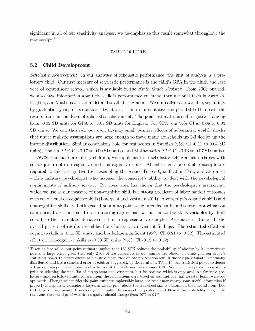
significant in all of our sensitivity analyses, we de-emphasize this result somewhat throughout the

manuscript.31

[TABLE 10 HERE]

5.2 Child Development

Scholastic Achievement. In our analyses of scholastic performance, the unit of analysis is a pre-

lottery child. Our first measure of scholastic performance is the child’s GPA in the ninth and last

year of compulsory school, which is available in the Ninth Grade Register. From 2003 onward,

we also have information about the child’s performance on mandatory national tests in Swedish,

English, and Mathematics administered to all ninth graders. We normalize each variable, separately

by graduation year, so its standard deviation is 1 in a representative sample. Table 11 reports the

results from our analyses of scholastic achievement. The point estimates are all negative, ranging

from -0.02 SD units for GPA to -0.08 SD units for English. For GPA, our 95% CI is -0.08 to 0.03

SD units. We can thus rule out even trivially small positive effects of substantial wealth shocks

that under realistic assumptions are large enough to move many households up 2-3 deciles up the

income distribution. Similar conclusions hold for test scores in Swedish (95% CI -0.11 to 0.04 SD

units), English (95% CI -0.17 to 0.00 SD units), and Mathematics (95% CI -0.13 to 0.07 SD units).

Skills. For male pre-lottery children, we supplement our scholastic achievement variables with

conscription data on cognitive and non-cognitive skills. At enlistment, potential conscripts are

required to take a cognitive test resembling the Armed Forces Qualification Test, and also meet

with a military psychologist who assesses the conscript’s ability to deal with the psychological

requirements of military service. Previous work has shown that the psychologist’s assessment,

which we use as our measure of non-cognitive skill, is a strong predictor of labor market outcomes

even conditional on cognitive skills (Lindqvist and Vestman 2011). A conscript’s cognitive skills and

non-cognitive skills are both graded on a nine-point scale intended to be a discrete approximation

to a normal distribution. In our outcome regressions, we normalize the skills variables by draft

cohort so their standard deviation is 1 in a representative sample. As shown in Table 11, the

overall pattern of results resembles the scholastic achievement findings. The estimated effect on

cognitive skills is -0.11 SD units, and borderline significant (95% CI -0.21 to -0.02). The estimated

effect on non-cognitive skills is -0.03 SD units (95% CI -0.19 to 0.12).

31 Taken at face value, our point estimate implies that 1M SEK reduces the probability of obesity by 2.1 percentagepoints, a large effect given that only 2.9% of the conscripts in our sample are obese. In hindsight, our study’sstatistical power to detect effects of plausible magnitude on obesity was too low. If the sample estimate is normallydistributed and has a standard error of 0.86, as suggested, by the results in Table 10, our statistical power to detecta 1 percentage point reduction in obesity risk at the 95% level was a mere 18%. We conducted power calculationsprior to selecting the final list of intergenerational outcomes, but for obesity, which is only available for male pre-lottery children followed until conscription, the calculations were based on assumptions that we later learnt were toooptimistic. Though we consider the point estimate implausibly large, the result may convey some useful information ifproperly interpreted. Consider a Bayesian whose prior about the true effect size is uniform on the interval from -1.00to 1.00 percentage points. Upon seeing our results, the mean of her posterior is -0.66 and the probability assigned tothe event that the sign of wealth is negative should change from 50% to 94%.

24

[TABLE 11 HERE]

5.3 Robustness

We conducted a number of additional sensitivity analyses of the main findings. Table A26 shows

that for binary outcomes, which include the obesity variable and the hospitalization variables, Pro-

bit marginal effects are of similar magnitude to the coeffi cients from our baseline linear probability

model. The estimated effect on premature births is no longer statistically significant in the Probit

specification. Table A26 also reports estimated effects on the drug consumption variables after

winsorization.

We also reran our main intergenerational analyses, dropping prizes below 10K, above 2M, or

above 4M. The results are shown in Tables A27-A28. Despite larger standard errors, the estimated

effect on hospitalizations is of similar magnitude and remains statistically significant in all specifi-

cations except the most restrictive specification in which we drop all prizes above 2M. We continue

to estimate negative effects on obesity risk in all three subsamples, but the effect is smaller and

not statistically significant when we exclude large prizes. The effect on premature birth is not

statistically significant when we drop prizes above 2M SEK or 4M SEK.

Tables A29 and A30 show results separately by lottery. The precision of the Triss-Monthly

estimates vary substantially across outcomes. For outcomes measured in conscripts (skills and

BMI), the number of male pre-lottery children observed in the right age span is too small to yield

meaningful results, and we do not report these estimates. For GPA, we continue to be able to rule

out modest positive effects of wealth even when the sample is restricted to Triss-Monthly (95% CI

-0.27 to 0.07). The estimated effect on obesity is strongest in Kombi, the sample with the highest

base rate of obesity risk. The estimated effect on five-year hospitalization risk is positive in each of

the individual lotteries, but only statistically distinguishable from 0 in the Triss-Lumpsum sample.

Finally, Table A35 shows results from our main outcome regressions with lottery prizes scaled by

the number of children. Overall, re-scaling lottery prizes this way does not result in large changes to

the coeffi cient estimates, although the absolute values of the estimated coeffi cients increase because

of the more compressed distribution of prizes. With the alternative scaling, the effect on 5-year

hospitalizations remains statistically significant, whereas the effect on obesity risk does not.

5.4 Heterogenous Effects

We conducted additional analyses in populations that some theories predict will exhibit heteroge-

neous responses: (1) household disposable income below or above the 25th percentile, (2) child’s

age below or above 9 at the time of the win, (3) mother or father won, (4) boys and girls. Psy-

chological and economic theories predict stronger responses to wealth in low-income households,

though the mechanism through which income translates into better outcomes differs (Becker and

Tomes 1976, Bradley and Corwyn 2002). Child age could be an important source of heterogene-

ity, for instance if there are more profitable investments opportunities in young children, or if it

takes time for positive effects to manifest themselves (for outcomes such as GPA and BMI, children

25

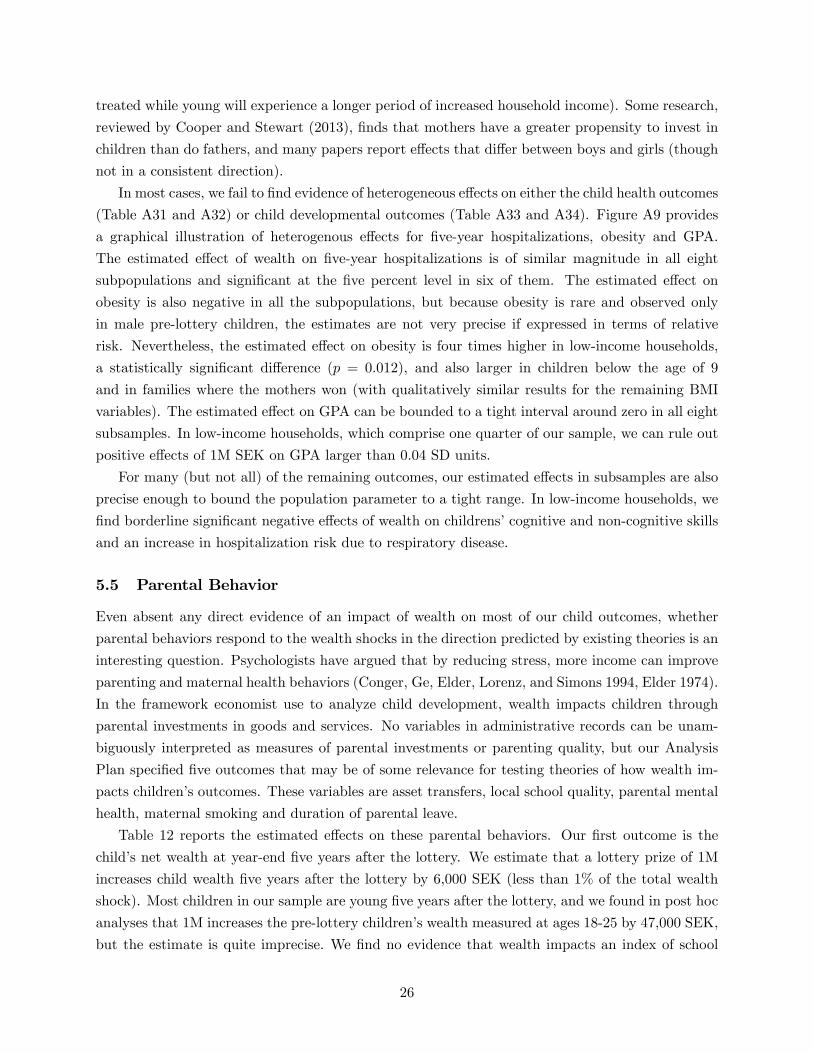
treated while young will experience a longer period of increased household income). Some research,

reviewed by Cooper and Stewart (2013), finds that mothers have a greater propensity to invest in

children than do fathers, and many papers report effects that differ between boys and girls (though

not in a consistent direction).

In most cases, we fail to find evidence of heterogeneous effects on either the child health outcomes

(Table A31 and A32) or child developmental outcomes (Table A33 and A34). Figure A9 provides

a graphical illustration of heterogenous effects for five-year hospitalizations, obesity and GPA.

The estimated effect of wealth on five-year hospitalizations is of similar magnitude in all eight

subpopulations and significant at the five percent level in six of them. The estimated effect on

obesity is also negative in all the subpopulations, but because obesity is rare and observed only

in male pre-lottery children, the estimates are not very precise if expressed in terms of relative

risk. Nevertheless, the estimated effect on obesity is four times higher in low-income households,

a statistically significant difference (p = 0.012), and also larger in children below the age of 9

and in families where the mothers won (with qualitatively similar results for the remaining BMI

variables). The estimated effect on GPA can be bounded to a tight interval around zero in all eight

subsamples. In low-income households, which comprise one quarter of our sample, we can rule out

positive effects of 1M SEK on GPA larger than 0.04 SD units.

For many (but not all) of the remaining outcomes, our estimated effects in subsamples are also

precise enough to bound the population parameter to a tight range. In low-income households, we

find borderline significant negative effects of wealth on childrens’cognitive and non-cognitive skills

and an increase in hospitalization risk due to respiratory disease.

5.5 Parental Behavior

Even absent any direct evidence of an impact of wealth on most of our child outcomes, whether

parental behaviors respond to the wealth shocks in the direction predicted by existing theories is an

interesting question. Psychologists have argued that by reducing stress, more income can improve

parenting and maternal health behaviors (Conger, Ge, Elder, Lorenz, and Simons 1994, Elder 1974).

In the framework economist use to analyze child development, wealth impacts children through

parental investments in goods and services. No variables in administrative records can be unam-

biguously interpreted as measures of parental investments or parenting quality, but our Analysis

Plan specified five outcomes that may be of some relevance for testing theories of how wealth im-

pacts children’s outcomes. These variables are asset transfers, local school quality, parental mental

health, maternal smoking and duration of parental leave.

Table 12 reports the estimated effects on these parental behaviors. Our first outcome is the

child’s net wealth at year-end five years after the lottery. We estimate that a lottery prize of 1M

increases child wealth five years after the lottery by 6,000 SEK (less than 1% of the total wealth

shock). Most children in our sample are young five years after the lottery, and we found in post hoc

analyses that 1M increases the pre-lottery children’s wealth measured at ages 18-25 by 47,000 SEK,

but the estimate is quite imprecise. We find no evidence that wealth impacts an index of school

26

quality32 and find reductions in both fathers’and mothers’mental health drug consumption of a

similar magnitude to what was observed in the adult analyses. Our two final parental behaviors

are days spent on parental leave during the child’s first three years and maternal smoking during

pregnancy. In mothers, we can reject positive effects of 1M SEK on parental leave larger than 13

days, a small effect given that the average mother claims 386 days of maternity leave benefits. The

estimated effect on maternal smoking is negative, indicating wealth reduces maternal smoking, but

it is not precisely estimated.

[TABLE 12]

6 Discussion

Observational studies consistently find strong gradients between markers for socioeconomic status

and health and child outcomes. But the causal processes that underlie these relationships remain

poorly understood (Baker and Stabile 2011, Currie 2009, Cutler, Lleras-Muney, and Vogl 2011,

Mayer 2010, Smith 1999, Deaton 2002). We contribute to this literature by providing credible and

statistically precise estimates of the causal impact of substantial wealth shocks on a rich set of

outcomes available in the administrative registers. For most outcomes, we report estimates that are

not statistically distinguishable from zero but often precise enough to bound the parameter being

estimated to a very tight range around the point estimate. Three possible exceptions to our overall

finding of zero effects are that wealth appears to improve adults’mental health, increase children’s

short-run hospitalization, and perhaps reduce their obesity risk.

There are limitations to what can be learnt about health and child achievement gradients by

studying the randomized assignment of large lottery prizes to Swedish lottery players. Sweden has

a publicly funded and universal health care system, and a schooling system that requires schools to

follow a national curriculum and prohibits them from charging tuition. An attempt to generalize

the results reported here to developing countries, where we have sound theoretical reasons to expect

larger effects and compelling evidence consistent with this expectation (Case 2004) would clearly

be inappropriate. Nor should one infer from our findings that large, positive, wealth shocks will

necessarily have small impacts on health care demand also in developed countries without universal

health care. However, health and child achievement gradients show up reliably across developed

countries with quite different institutional arrangements.33 Many theories of the gradients therefore

invoke causal mechanisms that plausibly operate in Sweden and across a wide range of other cultural

and policy environments.

To our knowledge, no previous study has exploited lottery-prize variation to estimate the causal

impact of wealth on children’s outcomes, and most existing quasi-experimental work examines

32We measure school quality as the average GPA, normalized by year, in the child’s graduating school in the year ofgraduation. The Analysis Plans describe how we handle a small number of students who attend schools from whichinformation about grades is either unavailable or baed on too few children to yield a reliable estimate of school quality.

33 For example, neither within- nor cross-country analyses find a strong relationship between the strength of the healthgradient and health care institutions (Cutler, Lleras-Muney, and Vogl 2011).

27

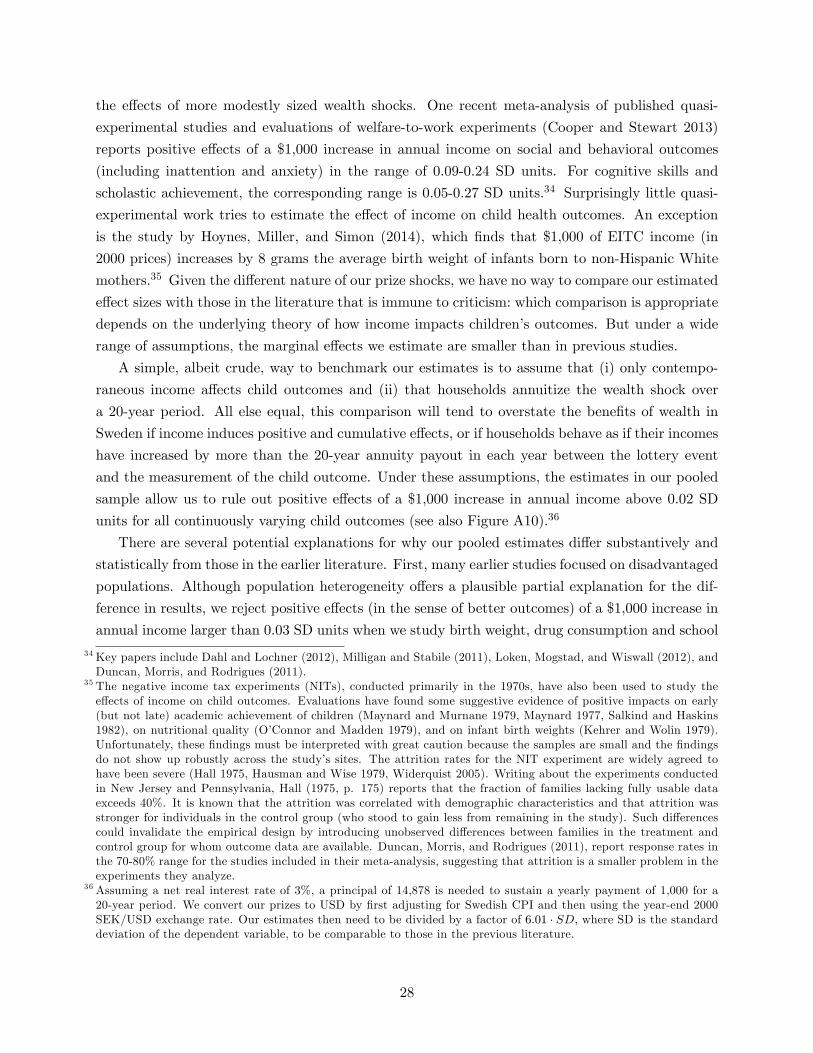
the effects of more modestly sized wealth shocks. One recent meta-analysis of published quasi-

experimental studies and evaluations of welfare-to-work experiments (Cooper and Stewart 2013)

reports positive effects of a $1,000 increase in annual income on social and behavioral outcomes

(including inattention and anxiety) in the range of 0.09-0.24 SD units. For cognitive skills and

scholastic achievement, the corresponding range is 0.05-0.27 SD units.34 Surprisingly little quasi-

experimental work tries to estimate the effect of income on child health outcomes. An exception

is the study by Hoynes, Miller, and Simon (2014), which finds that $1,000 of EITC income (in

2000 prices) increases by 8 grams the average birth weight of infants born to non-Hispanic White

mothers.35 Given the different nature of our prize shocks, we have no way to compare our estimated

effect sizes with those in the literature that is immune to criticism: which comparison is appropriate

depends on the underlying theory of how income impacts children’s outcomes. But under a wide

range of assumptions, the marginal effects we estimate are smaller than in previous studies.

A simple, albeit crude, way to benchmark our estimates is to assume that (i) only contempo-

raneous income affects child outcomes and (ii) that households annuitize the wealth shock over

a 20-year period. All else equal, this comparison will tend to overstate the benefits of wealth in

Sweden if income induces positive and cumulative effects, or if households behave as if their incomes

have increased by more than the 20-year annuity payout in each year between the lottery event

and the measurement of the child outcome. Under these assumptions, the estimates in our pooled

sample allow us to rule out positive effects of a $1,000 increase in annual income above 0.02 SD

units for all continuously varying child outcomes (see also Figure A10).36

There are several potential explanations for why our pooled estimates differ substantively and

statistically from those in the earlier literature. First, many earlier studies focused on disadvantaged

populations. Although population heterogeneity offers a plausible partial explanation for the dif-

ference in results, we reject positive effects (in the sense of better outcomes) of a $1,000 increase in

annual income larger than 0.03 SD units when we study birth weight, drug consumption and school

34Key papers include Dahl and Lochner (2012), Milligan and Stabile (2011), Loken, Mogstad, and Wiswall (2012), andDuncan, Morris, and Rodrigues (2011).

35 The negative income tax experiments (NITs), conducted primarily in the 1970s, have also been used to study theeffects of income on child outcomes. Evaluations have found some suggestive evidence of positive impacts on early(but not late) academic achievement of children (Maynard and Murnane 1979, Maynard 1977, Salkind and Haskins1982), on nutritional quality (O’Connor and Madden 1979), and on infant birth weights (Kehrer and Wolin 1979).Unfortunately, these findings must be interpreted with great caution because the samples are small and the findingsdo not show up robustly across the study’s sites. The attrition rates for the NIT experiment are widely agreed tohave been severe (Hall 1975, Hausman and Wise 1979, Widerquist 2005). Writing about the experiments conductedin New Jersey and Pennsylvania, Hall (1975, p. 175) reports that the fraction of families lacking fully usable dataexceeds 40%. It is known that the attrition was correlated with demographic characteristics and that attrition wasstronger for individuals in the control group (who stood to gain less from remaining in the study). Such differencescould invalidate the empirical design by introducing unobserved differences between families in the treatment andcontrol group for whom outcome data are available. Duncan, Morris, and Rodrigues (2011), report response rates inthe 70-80% range for the studies included in their meta-analysis, suggesting that attrition is a smaller problem in theexperiments they analyze.

36 Assuming a net real interest rate of 3%, a principal of 14,878 is needed to sustain a yearly payment of 1,000 for a20-year period. We convert our prizes to USD by first adjusting for Swedish CPI and then using the year-end 2000SEK/USD exchange rate. Our estimates then need to be divided by a factor of 6.01 · SD, where SD is the standarddeviation of the dependent variable, to be comparable to those in the previous literature.

28

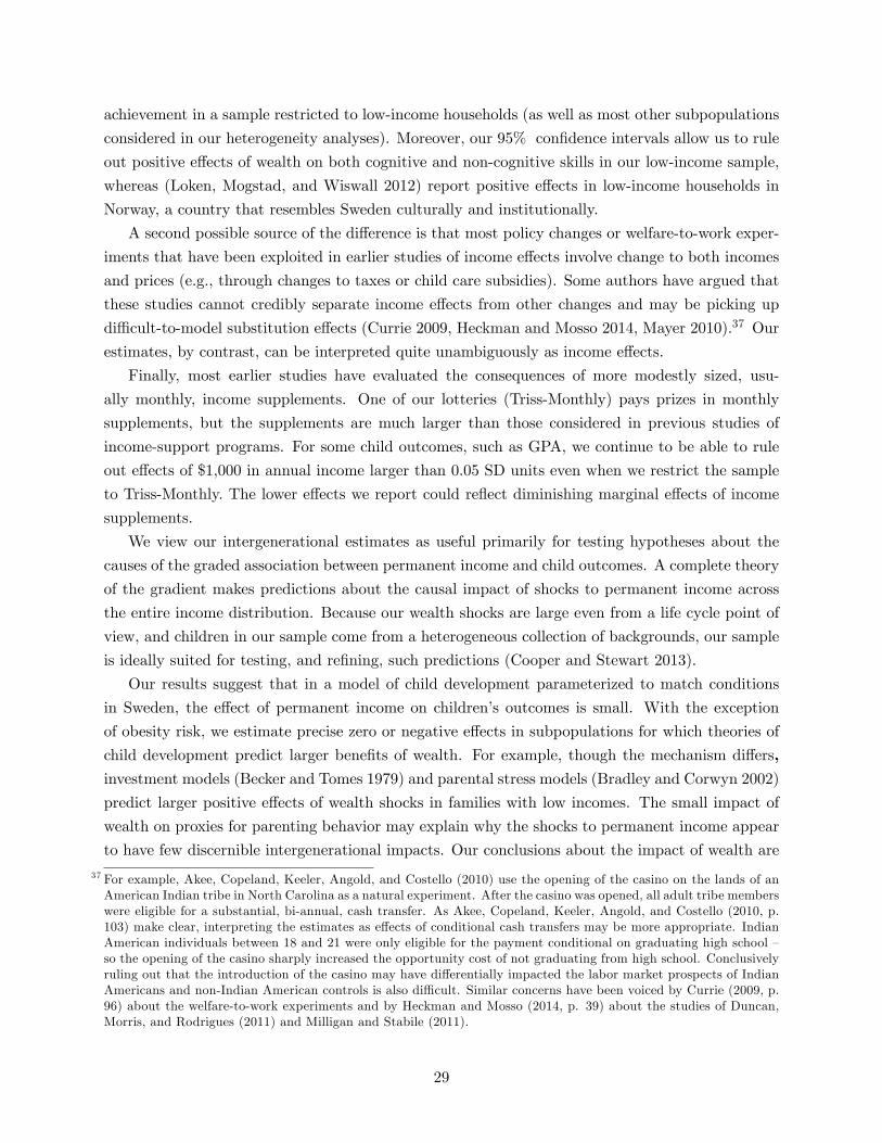
achievement in a sample restricted to low-income households (as well as most other subpopulations

considered in our heterogeneity analyses). Moreover, our 95% confidence intervals allow us to rule

out positive effects of wealth on both cognitive and non-cognitive skills in our low-income sample,

whereas (Loken, Mogstad, and Wiswall 2012) report positive effects in low-income households in

Norway, a country that resembles Sweden culturally and institutionally.

A second possible source of the difference is that most policy changes or welfare-to-work exper-

iments that have been exploited in earlier studies of income effects involve change to both incomes

and prices (e.g., through changes to taxes or child care subsidies). Some authors have argued that

these studies cannot credibly separate income effects from other changes and may be picking up

diffi cult-to-model substitution effects (Currie 2009, Heckman and Mosso 2014, Mayer 2010).37 Our

estimates, by contrast, can be interpreted quite unambiguously as income effects.

Finally, most earlier studies have evaluated the consequences of more modestly sized, usu-

ally monthly, income supplements. One of our lotteries (Triss-Monthly) pays prizes in monthly

supplements, but the supplements are much larger than those considered in previous studies of

income-support programs. For some child outcomes, such as GPA, we continue to be able to rule

out effects of $1,000 in annual income larger than 0.05 SD units even when we restrict the sample

to Triss-Monthly. The lower effects we report could reflect diminishing marginal effects of income

supplements.

We view our intergenerational estimates as useful primarily for testing hypotheses about the

causes of the graded association between permanent income and child outcomes. A complete theory

of the gradient makes predictions about the causal impact of shocks to permanent income across

the entire income distribution. Because our wealth shocks are large even from a life cycle point of

view, and children in our sample come from a heterogeneous collection of backgrounds, our sample

is ideally suited for testing, and refining, such predictions (Cooper and Stewart 2013).

Our results suggest that in a model of child development parameterized to match conditions

in Sweden, the effect of permanent income on children’s outcomes is small. With the exception

of obesity risk, we estimate precise zero or negative effects in subpopulations for which theories of

child development predict larger benefits of wealth. For example, though the mechanism differs,investment models (Becker and Tomes 1979) and parental stress models (Bradley and Corwyn 2002)

predict larger positive effects of wealth shocks in families with low incomes. The small impact of

wealth on proxies for parenting behavior may explain why the shocks to permanent income appear

to have few discernible intergenerational impacts. Our conclusions about the impact of wealth are

37 For example, Akee, Copeland, Keeler, Angold, and Costello (2010) use the opening of the casino on the lands of anAmerican Indian tribe in North Carolina as a natural experiment. After the casino was opened, all adult tribe memberswere eligible for a substantial, bi-annual, cash transfer. As Akee, Copeland, Keeler, Angold, and Costello (2010, p.103) make clear, interpreting the estimates as effects of conditional cash transfers may be more appropriate. IndianAmerican individuals between 18 and 21 were only eligible for the payment conditional on graduating high school —so the opening of the casino sharply increased the opportunity cost of not graduating from high school. Conclusivelyruling out that the introduction of the casino may have differentially impacted the labor market prospects of IndianAmericans and non-Indian American controls is also diffi cult. Similar concerns have been voiced by Currie (2009, p.96) about the welfare-to-work experiments and by Heckman and Mosso (2014, p. 39) about the studies of Duncan,Morris, and Rodrigues (2011) and Milligan and Stabile (2011).

29

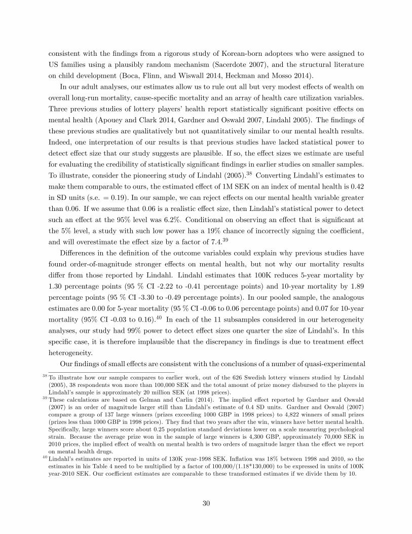
consistent with the findings from a rigorous study of Korean-born adoptees who were assigned to

US families using a plausibly random mechanism (Sacerdote 2007), and the structural literature

on child development (Boca, Flinn, and Wiswall 2014, Heckman and Mosso 2014).

In our adult analyses, our estimates allow us to rule out all but very modest effects of wealth on

overall long-run mortality, cause-specific mortality and an array of health care utilization variables.

Three previous studies of lottery players’health report statistically significant positive effects on

mental health (Apouey and Clark 2014, Gardner and Oswald 2007, Lindahl 2005). The findings of

these previous studies are qualitatively but not quantitatively similar to our mental health results.

Indeed, one interpretation of our results is that previous studies have lacked statistical power to

detect effect size that our study suggests are plausible. If so, the effect sizes we estimate are useful

for evaluating the credibility of statistically significant findings in earlier studies on smaller samples.

To illustrate, consider the pioneering study of Lindahl (2005).38 Converting Lindahl’s estimates to

make them comparable to ours, the estimated effect of 1M SEK on an index of mental health is 0.42

in SD units (s.e. = 0.19). In our sample, we can reject effects on our mental health variable greater

than 0.06. If we assume that 0.06 is a realistic effect size, then Lindahl’s statistical power to detect

such an effect at the 95% level was 6.2%. Conditional on observing an effect that is significant at

the 5% level, a study with such low power has a 19% chance of incorrectly signing the coeffi cient,

and will overestimate the effect size by a factor of 7.4.39

Differences in the definition of the outcome variables could explain why previous studies have

found order-of-magnitude stronger effects on mental health, but not why our mortality results

differ from those reported by Lindahl. Lindahl estimates that 100K reduces 5-year mortality by

1.30 percentage points (95 % CI -2.22 to -0.41 percentage points) and 10-year mortality by 1.89

percentage points (95 % CI -3.30 to -0.49 percentage points). In our pooled sample, the analogous

estimates are 0.00 for 5-year mortality (95 % CI -0.06 to 0.06 percentage points) and 0.07 for 10-year

mortality (95% CI -0.03 to 0.16).40 In each of the 11 subsamples considered in our heterogeneity

analyses, our study had 99% power to detect effect sizes one quarter the size of Lindahl’s. In this

specific case, it is therefore implausible that the discrepancy in findings is due to treatment effect

heterogeneity.

Our findings of small effects are consistent with the conclusions of a number of quasi-experimental

38 To illustrate how our sample compares to earlier work, out of the 626 Swedish lottery winners studied by Lindahl(2005), 38 respondents won more than 100,000 SEK and the total amount of prize money disbursed to the players inLindahl’s sample is approximately 20 million SEK (at 1998 prices).

39 These calculations are based on Gelman and Carlin (2014). The implied effect reported by Gardner and Oswald(2007) is an order of magnitude larger still than Lindahl’s estimate of 0.4 SD units. Gardner and Oswald (2007)compare a group of 137 large winners (prizes exceeding 1000 GBP in 1998 prices) to 4,822 winners of small prizes(prizes less than 1000 GBP in 1998 prices). They find that two years after the win, winners have better mental health.Specifically, large winners score about 0.25 population standard deviations lower on a scale measuring psychologicalstrain. Because the average prize won in the sample of large winners is 4,300 GBP, approximately 70,000 SEK in2010 prices, the implied effect of wealth on mental health is two orders of magnitude larger than the effect we reporton mental health drugs.

40 Lindahl’s estimates are reported in units of 130K year-1998 SEK. Inflation was 18% between 1998 and 2010, so theestimates in his Table 4 need to be multiplied by a factor of 100,000/(1.18*130,000) to be expressed in units of 100Kyear-2010 SEK. Our coeffi cient estimates are comparable to these transformed estimates if we divide them by 10.

30

papers using natural experiments other than lotteries (Erixson 2014, Frijters, Haisken-DeNew, and

Shields 2005, Meer, Miller, and Rosen 2003, Snyder and Evans 2006, Stowasser, Heiss, McFadden,

and Winter 2011). Economists, placing the most weight on this evidence, have often concluded

that omitted variables and reverse causation from health to wealth primarily explain the gradients

between income and health (Chandra and Vogl 2010, Deaton 2003, Smith 1999) whereas epidemiol-

ogists frequently point to the substantial health-wealth correlations —and their apparent robustness

to the inclusion of a large set of controls — in support of their positions (Marmot 1994). Our es-

timates reinforce economists’skepticism.41 Overall, we find no strong evidence of heterogeneous

effects, though we find hints that wealth increases mortality risk in some groups, such as individuals

above the age of 70 Snyder and Evans (2006, see also).

We find little support for what we take to be the predictions from the epidemiological literature

about the impacts of wealth. The suggestive mental health findings are consistent with income

conveying some psychosocial benefits (Adler and Newman 2002, Marmot and Wilkinson 2009),

but we find no evidence that these benefits translate into improved autoimmune or cardiovascular

health. Nor do we find positive effects on health outcomes in individuals with low socioeconomic

status. In our mortality analyses, we find no evidence for a gradual accumulation of positive effects

or that wealth confers large benefits to members of groups that the epidemiological literature has

traditionally identified as vulnerable.

The identification of the causal processes that produce the relationships between SES and health

over the life cycle is fraught with methodological hazards. One such hazard is that treating SES

as a unified concept may obfuscate the heterogenous effects of its various dimensions over the

lifecycle (Cutler, Lleras-Muney, and Vogl 2011, Deaton 2002). Though no silver bullet can answer

these pressing research questions, studies of lottery players are one attractive research strategy for

understanding how economic resources, one important dimension of SES, impact health and child

outcomes (Smith 1999, Mayer 1998). We find that overall, the effects of substantial, positive, wealth

shocks are small, both in the aggregate, and in subsamples. Our results are not incompatible with

the existence of substantial causal pathways from some dimensions of SES to health, but may help

narrow the set of hypotheses about the causes of the gradients that should be considered plausible.

References

Adams, P., M. D. Hurd, D. McFadden, A. Merrill, and T. Ribeiro (2003): “Healthy,

Wealthy, and Wise? Tests for Direct Causal Paths Between Health and Socioeconomic Sta-

tus,”Journal of Econometrics, 112, 3—56.

Adda, J., J. Banks, and H.-M. von Gaudecker (2009): “The Impact of Income Shocks

41 As we have repeatedly emphasized, the prize-distribution in our data prevents us from estimating with the effects ofvery modest wealth shocks (of the order a few thousand dollars). Our findings are thus not at odds with a US literaturethat shows a within-month mortality spike in connection with receipt of government transfer payments (Dobkin andPuller 2007, Evans and Moore 2011, Evans and Moore 2012). These spikes appear to be driven by increases ineconomic activity and the consumption of health-impairing substances. Similar spikes have been documented inSwedish data (Andersson, Lundborg, and Vikström 2014)

31

on Health: Evidence from Cohort Data,” Journal of the European Economic Association,

7(3329), 1361—1399.

Adler, N. E., and K. Newman (2002): “Socioeconomic Disparities In Health: Pathways And

Policies,”Health Affairs, 21(2), 60—76.

Akee, R. K., W. Copeland, G. Keeler, A. Angold, and E. J. Costello (2010): “Par-

entsŠ Incomes and Children’s Outcomes: A Quasi-Experiment Using Transfer Payments from

Casino Profits,”American Economic Journal: Applied Economics, 2(1), 86—115.

Andersson, E., P. Lundborg, and J. Vikström (2014): “Income Receipt and Mortality - Ev-

idence from Swedish Public Sector Employees,”Department of Economics, Lund University

Working Paper No 32.

Apouey, B., and A. E. Clark (2014): “Winning Big but Feeling No Better? The Effect of

Lottery Prizes on Physical and Mental Health,”Health Economics, DOI 10.1002/hec.3035.

Baker, M., and M. Stabile (2011): “Determinants of Health in Childhood,” in The Oxford

Handbook of Health Economics. Oxford University Press.

Becker, G. S., and N. Tomes (1976): “Child Endowments and the Quantity and Quality of

Children,”Journal of Political Economy, 84(S4), S143—S162.

Becker, G. S., and N. Tomes (1979): “An Equilibrium Theory of the Distribution of Income

and Intergenerational Mobility,”Journal of Political, 87(6), 1153—1189.

Boca, D. D., C. Flinn, and M. Wiswall (2014): “Household Choices and Child Development,”

Review of Economic Studies, 81(1), 137—185.

Bradley, R. H., and R. F. Corwyn (2002): “Socioeconomic Status and Child Development,”

Annual Review of Psychology, 53, 371—99.

Brooks-Gunn, J., and G. J. Duncan (1997): “The Effects of Poverty on Children,”Future of

Children, 7(2), 55—71.

Brunner, E. (1997): “Stress and the Biology of Inequality,”British Medical Journal, 314(7092),

1472—1476.

Case, A. (2004): “Does Money Protect Health Status? Evidence from South African Pensions,”

in Perspectives on the Economics of Aging, ed. by D. A. Wise, pp. 287—311. University of

Chicago Press.

Cesarini, D., E. Lindqvist, M. Notowidigdo, and R. Östling (2015): “The Effect of Wealth

on Individual and Household Labor Supply: Evidence from Swedish Lotteries,”IFN Working

Paper.

Chandra, A., and T. S. Vogl (2010): “Rising up with Shoe Leather? A Comment on "Fair

Society, Healthy Lives (The Marmot Review)",”Social Science & Medicine, 71, 1227—1230.

32

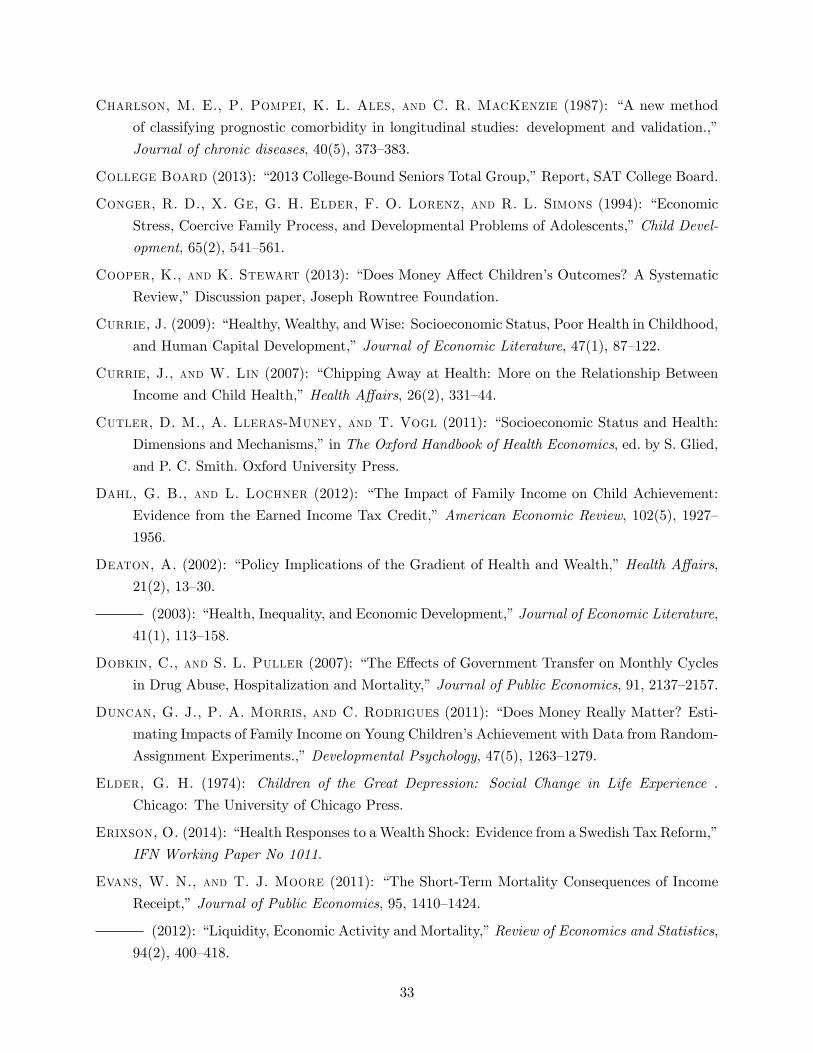
Charlson, M. E., P. Pompei, K. L. Ales, and C. R. MacKenzie (1987): “A new method

of classifying prognostic comorbidity in longitudinal studies: development and validation.,”

Journal of chronic diseases, 40(5), 373—383.

College Board (2013): “2013 College-Bound Seniors Total Group,”Report, SAT College Board.

Conger, R. D., X. Ge, G. H. Elder, F. O. Lorenz, and R. L. Simons (1994): “Economic

Stress, Coercive Family Process, and Developmental Problems of Adolescents,”Child Devel-

opment, 65(2), 541—561.

Cooper, K., and K. Stewart (2013): “Does Money Affect Children’s Outcomes? A Systematic

Review,”Discussion paper, Joseph Rowntree Foundation.

Currie, J. (2009): “Healthy, Wealthy, andWise: Socioeconomic Status, Poor Health in Childhood,

and Human Capital Development,”Journal of Economic Literature, 47(1), 87—122.

Currie, J., and W. Lin (2007): “Chipping Away at Health: More on the Relationship Between

Income and Child Health,”Health Affairs, 26(2), 331—44.

Cutler, D. M., A. Lleras-Muney, and T. Vogl (2011): “Socioeconomic Status and Health:

Dimensions and Mechanisms,”in The Oxford Handbook of Health Economics, ed. by S. Glied,

and P. C. Smith. Oxford University Press.

Dahl, G. B., and L. Lochner (2012): “The Impact of Family Income on Child Achievement:

Evidence from the Earned Income Tax Credit,”American Economic Review, 102(5), 1927—

1956.

Deaton, A. (2002): “Policy Implications of the Gradient of Health and Wealth,”Health Affairs,

21(2), 13—30.

(2003): “Health, Inequality, and Economic Development,”Journal of Economic Literature,

41(1), 113—158.

Dobkin, C., and S. L. Puller (2007): “The Effects of Government Transfer on Monthly Cycles

in Drug Abuse, Hospitalization and Mortality,”Journal of Public Economics, 91, 2137—2157.

Duncan, G. J., P. A. Morris, and C. Rodrigues (2011): “Does Money Really Matter? Esti-

mating Impacts of Family Income on Young Children’s Achievement with Data from Random-

Assignment Experiments.,”Developmental Psychology, 47(5), 1263—1279.

Elder, G. H. (1974): Children of the Great Depression: Social Change in Life Experience .

Chicago: The University of Chicago Press.

Erixson, O. (2014): “Health Responses to a Wealth Shock: Evidence from a Swedish Tax Reform,”

IFN Working Paper No 1011.

Evans, W. N., and T. J. Moore (2011): “The Short-Term Mortality Consequences of Income

Receipt,”Journal of Public Economics, 95, 1410—1424.

(2012): “Liquidity, Economic Activity and Mortality,”Review of Economics and Statistics,

94(2), 400—418.

33

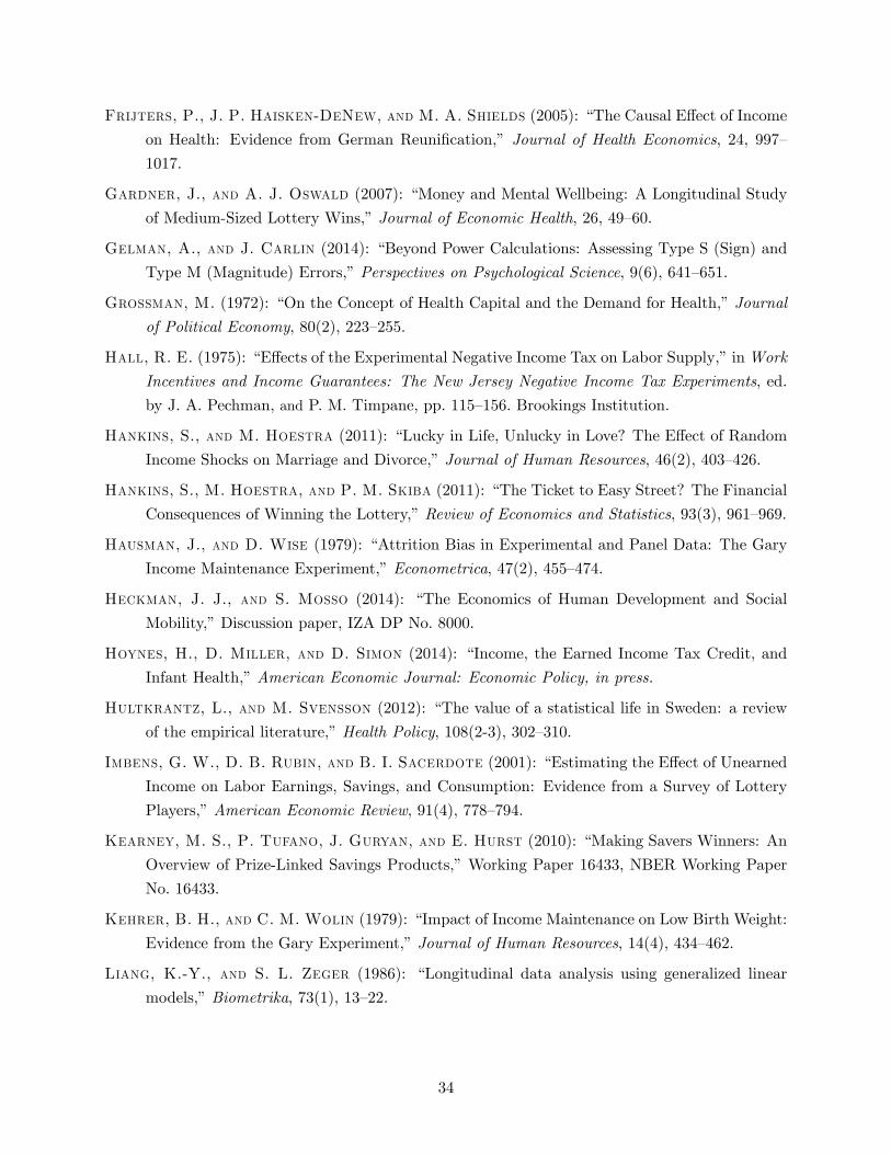
Frijters, P., J. P. Haisken-DeNew, and M. A. Shields (2005): “The Causal Effect of Income

on Health: Evidence from German Reunification,” Journal of Health Economics, 24, 997—

1017.

Gardner, J., and A. J. Oswald (2007): “Money and Mental Wellbeing: A Longitudinal Study

of Medium-Sized Lottery Wins,”Journal of Economic Health, 26, 49—60.

Gelman, A., and J. Carlin (2014): “Beyond Power Calculations: Assessing Type S (Sign) and

Type M (Magnitude) Errors,”Perspectives on Psychological Science, 9(6), 641—651.

Grossman, M. (1972): “On the Concept of Health Capital and the Demand for Health,”Journal

of Political Economy, 80(2), 223—255.

Hall, R. E. (1975): “Effects of the Experimental Negative Income Tax on Labor Supply,”inWork

Incentives and Income Guarantees: The New Jersey Negative Income Tax Experiments, ed.

by J. A. Pechman, and P. M. Timpane, pp. 115—156. Brookings Institution.

Hankins, S., and M. Hoestra (2011): “Lucky in Life, Unlucky in Love? The Effect of Random

Income Shocks on Marriage and Divorce,”Journal of Human Resources, 46(2), 403—426.

Hankins, S., M. Hoestra, and P. M. Skiba (2011): “The Ticket to Easy Street? The Financial

Consequences of Winning the Lottery,”Review of Economics and Statistics, 93(3), 961—969.

Hausman, J., and D. Wise (1979): “Attrition Bias in Experimental and Panel Data: The Gary

Income Maintenance Experiment,”Econometrica, 47(2), 455—474.

Heckman, J. J., and S. Mosso (2014): “The Economics of Human Development and Social

Mobility,”Discussion paper, IZA DP No. 8000.

Hoynes, H., D. Miller, and D. Simon (2014): “Income, the Earned Income Tax Credit, and

Infant Health,”American Economic Journal: Economic Policy, in press.

Hultkrantz, L., and M. Svensson (2012): “The value of a statistical life in Sweden: a review

of the empirical literature,”Health Policy, 108(2-3), 302—310.

Imbens, G. W., D. B. Rubin, and B. I. Sacerdote (2001): “Estimating the Effect of Unearned

Income on Labor Earnings, Savings, and Consumption: Evidence from a Survey of Lottery

Players,”American Economic Review, 91(4), 778—794.

Kearney, M. S., P. Tufano, J. Guryan, and E. Hurst (2010): “Making Savers Winners: An

Overview of Prize-Linked Savings Products,”Working Paper 16433, NBER Working Paper

No. 16433.

Kehrer, B. H., and C. M. Wolin (1979): “Impact of Income Maintenance on Low Birth Weight:

Evidence from the Gary Experiment,”Journal of Human Resources, 14(4), 434—462.

Liang, K.-Y., and S. L. Zeger (1986): “Longitudinal data analysis using generalized linear

models,”Biometrika, 73(1), 13—22.

34

Lindahl, M. (2005): “Estimating the Effect of Income on Health and Mortality Using Lottery

Prizes as an Exogenous Source of Variation in Income,”Journal of Human Resources, 40(1),

144—168.

Lindqvist, E., and R. Vestman (2011): “The Labor Market Returns to Cognitive and Noncogni-

tive Ability: Evidence from the Swedish Enlistment,”American Economic Journal: Applied

Economics, 3(1), 101—128.

Loken, K. V., M. Mogstad, and M. Wiswall (2012): “What Linear Estimators Miss: The

Effects of Family Income on Child Outcomes,”American Economic Journal: Applied Eco-

nomics, 4(2), 1—35.

Majo, M. C., and A. V. Soest (2011): “Income and Health Care Utilization Among the 50+ in

Europe and the US,”Netspar Discussion Paper 06/2011-065.

Marmot, M. (1994): “Social Differentials in Health Within and Between Populations,”Daedalus,

123, 197—216.

Marmot, M., and R. Wilkinson (2009): Social Determinants of Health. Oxford University

Press.

Mayer, S. E. (1998): What Money Can’t Buy: Family Income and Children’s Life Chances.

Harvard University Press, Cambridge, MA, first edn.

(2010): “Revisiting an old question : How much does parental income affect child out-

comes?,”Focus, 27(2), 21—26.

Maynard, R. A. (1977): “The effects of the rural income maintenance experiment on the school

performance of children,”American Economic Review, 67(1), 370—375.

Maynard, R. A., and R. J. Murnane (1979): “The Effects of a Negative Income Tax on School

Performance : Results of an Experiment,”Journal of Human Resources, 14(4), 463—476.

Meer, J., D. L. Miller, and H. S. Rosen (2003): “Exploring the Health-Wealth Nexus,”

Journal of Health Economics, 22, 713—730.

Milligan, K., andM. Stabile (2011): “Do Child Tax Benefits Affect the Well-Being of Children?

Evidence from Canadian Child Benefit Expansions,”American Economic Journal: Economic

Policy, 3(3), 175—205.

Morken, N.-H., K. Kallen, H. Hagberga, and B. Jacobsson (2005): “Preterm birth in Swe-

den 1973-2001: rate, subgroups, and effect of changing patterns in multiple births, maternal

age, and smoking.,”Acta Obstetricia et Gynecologica Scandinavica, 84(6), 558—565.

Newacheck, P. W., and N. Halfon (1998): “Prevalence and Impact of Disabling Chronic

Conditions in Childhood,”American Journal of Public Health, 88(4), 610—617.

O’Connor, J. F., and J. P. Madden (1979): “The Negative Income Tax and the Quality of

Dietary Intake,”Journal of Human Resources, 14(4), 507—517.

35

Sacerdote, B. (2007): “How Large are the Effects from Changes in Family Environment? A

Study of Korean American Adoptees,”Quarterly Journal of Economics, 122(1), 119—157.

Salkind, N., and R. Haskins (1982): “Negative Income Tax The Impact on Children from

Low-Income Families,”Journal of Family Issues, 3(2), 165—180.

Semyonov, M., N. Lewin-Epstein, and D. Maskileyson (2013): “Where Wealth Matters

More for Health: The Wealth-Health Gradient in 16 Countries,”Social Science & Medicine,

81, 10—17.

Smith, J. (2007): “The Impact of Social Economic Status on Health Over the Life-Course,”Journal

of Human Resources, 42, 739—764.

Smith, J. P. (1999): “Healthy Bodies and Thick Wallets: The Dual Relation between Health and

Economic Status,”Journal of Economic Perspectives, 13(2), 145—166.

Smith, J. P. (2009): “The Impact of Childhood Health on Adult Labor Market Outcomes,”Review

of Economics and Statistics, 91(3), 478—489.

Snyder, S. E., and W. N. Evans (2006): “The Effect of Income on Mortality: Evidence from

the Social Security Notch,”Review of Economics and Statistics, 88, 482—495.

Stansfeld, S. A., R. Fuhrer, M. J. Shipley, and M. G. Marmot (2002): “Psychological

Distress as a Risk Factor for Coronary Heart Disease in the Whitehall II Study,”International

Journal of Epidemiology, 31(1), 248—255.

Stowasser, T., F. Heiss, D. McFadden, and J. Winter (2011): “Healthy, Wealthy and Wise?’

Revisited: An Analysis of the Causal Pathways from Socio-economic Status to Health,”

NBER Working Paper No. 17273.

van Kippersluis, H., and T. J. Galama (2013): “Why the Rich Drink More, but Smoke Less:

the Impact of Wealth on Health Behavior,”Tinbergen Institute Discussion Paper 13-035.

Widerquist, K. (2005): “A Failure to Communicate: What (if Anything) Can We Learn From

the Negative Income Tax Experiments?,”The Journal of Socio-Economics, 34(1), 49—81.

Williams, D. R. (1990): “Socioeconomic Differentials in Health: A Review and Redirection,”

Social Psychology Quarterly, 53, 81—99.

36

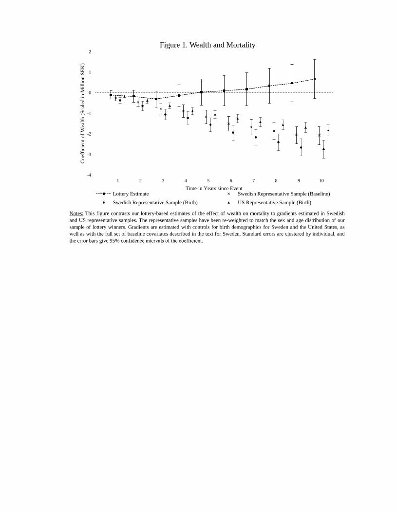
Notes: This figure contrasts our lottery-based estimates of the effect of wealth on mortality to gradients estimated in Swedishand US representative samples. The representative samples have been re-weighted to match the sex and age distribution of oursample of lottery winners. Gradients are estimated with controls for birth demographics for Sweden and the United States, aswell as with the full set of baseline covariates described in the text for Sweden. Standard errors are clustered by individual, andthe error bars give 95% con�fidence intervals of the coefficient.

-4

-3

-2

-1

0

1

2

0 1 2 3 4 5 6 7 8 9 10

Coe

ffici

ent o

f Wea

lth (S

cale

d in

Mill

ion

SEK

)

Time in Years since Event

Figure 1. Wealth and Mortality

Lottery Estimate Swedish Representative Sample (Baseline)Swedish Representative Sample (Birth) US Representative Sample (Birth)

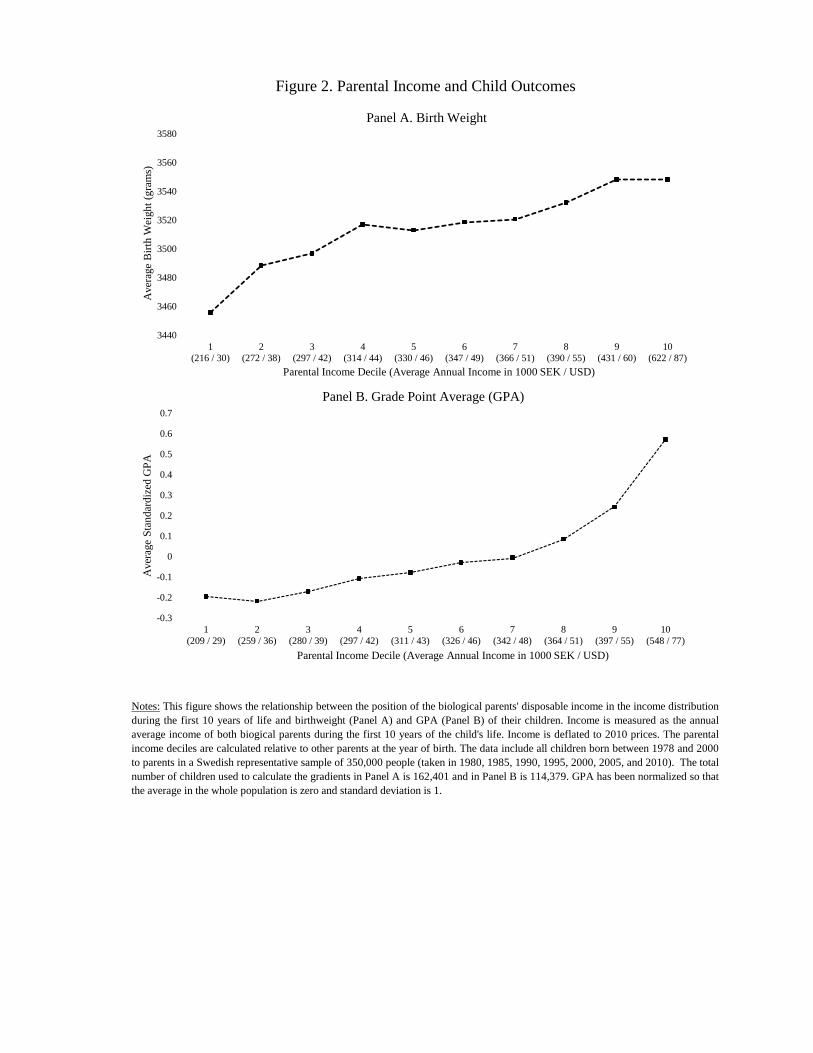
Figure 2. Parental Income and Child Outcomes

Notes: This figure shows the relationship between the position of the biological parents' disposable income in the income distributionduring the first 10 years of life and birthweight (Panel A) and GPA (Panel B) of their children. Income is measured as the annualaverage income of both biogical parents during the first 10 years of the child's life. Income is deflated to 2010 prices. The parentalincome deciles are calculated relative to other parents at the year of birth. The data include all children born between 1978 and 2000to parents in a Swedish representative sample of 350,000 people (taken in 1980, 1985, 1990, 1995, 2000, 2005, and 2010). The totalnumber of children used to calculate the gradients in Panel A is 162,401 and in Panel B is 114,379. GPA has been normalized so thatthe average in the whole population is zero and standard deviation is 1.

3440

3460

3480

3500

3520

3540

3560

3580

1(216 / 30)

2(272 / 38)

3(297 / 42)

4(314 / 44)

5(330 / 46)

6(347 / 49)

7(366 / 51)

8(390 / 55)

9(431 / 60)

10(622 / 87)

Ave

rage

Birt

h W

eigh

t (gr

ams)

Parental Income Decile (Average Annual Income in 1000 SEK / USD)

Panel A. Birth Weight

-0.3

-0.2

-0.1

0

0.1

0.2

0.3

0.4

0.5

0.6

0.7

1(209 / 29)

2(259 / 36)

3(280 / 39)

4(297 / 42)

5(311 / 43)

6(326 / 46)

7(342 / 48)

8(364 / 51)

9(397 / 55)

10(548 / 77)

Ave

rage

Sta

ndar

dize

d G

PA

Parental Income Decile (Average Annual Income in 1000 SEK / USD)

Panel B. Grade Point Average (GPA)

Register Name (Period) Unit of Observation Outcomes Measured

Cause of Death (1952-)* Death Event Up to 24 years post lottery

Conscription (1969-)** ~18-Year Old Male At Age ~18Medical Birth (1973-)** Infant At BirthNinth Grade (1988-)** Ninth-Grade Student At Age ~15

National Tests (2003-)** Ninth-Grade Student At Age ~15

Patient (1987-) Hospitalization Event Up to 10 years post lottery

Prescribed Drug (2006-) Drug Purchase 2006-2010

Birth Demographics Health CharacteristicsAge 1 if Hospitalized Age2 1 if Hospitalized ≥ 7 daysAge3 1 if Hospitalized for Cancer1 if Female 1 if Hospitalized for Respiratory 1 if Born in Nordic Country 1 if Hospitalized for Circulatory

Charlson Index

1 if College-Graduate# Children

Entry & Discharge Dates, Diagnoses (ICD)

Date, Type (ATC), Quantity (DDD)

Notes: The upper panel gives summary background information about the registers used to construct our outcome variables. BMI: BodyMass Index. ATC: Anatomical Therapeutic Chemical Classification. ICD: Internal Classification of Diseases. DDD: Defined Daily Doses.The lower panel defines a set of demographic and health characteristics that will be used throughout the paper. Labor income is measured inthousands of SEK (at 2010 prices). All hospitalization variables are binary and defined over the preceding five years. Additional details onthe construction of the Charlson index and the classification of causes of hospitalization are available in the Online Appendix (sections 6.3and 6.5). * used in intergenerational analyses only, ** adult only.

Income/1001 if Retired**

Other Demographics1 if Married

Table 1. Overview of Main Registers and Control Variables

Panel A. Registers Used to Generate Main Outcome Variables

Panel B. Definition of Baseline Controls

Data Description

Date and Cause of Death (ICD)Cog and Noncog Skills, BMIBirth Weight, GestationGPATest Scores in English, Mathematics, Swedish

Lottery Period Type Adult Analyses Child Analyses Adult Pre-lottery

Post-lottery

PLS Fixed Prizes 1986-2003 Lumpsum Year-Month ×

# Fixed PrizesYear-Month × # Fixed

Prizes × # Children 228 487 400

PLS Odds Prizes 1986-1994 Lumpsum Year-Month ×

# Prizes × # Tickets Excluded 1881 0 0

Kombi 1998-2010 Lumpsum Year-Month × Account

BalanceYear-Month × Account Balance × # Children 262 51 6

Triss-Lumpsum 1994-2010 Lumpsum Year × Prize Plan Year × Prize Plan ×

# Children 18 67 51

Triss-Monthly 1997-2010

Monthly Installments Year × Prize Plan Year × Prize Plan ×

# Children 19 37 12

Table 2. Overview of Identification Strategy

Notes: This table provides a summary overview of the identification strategies used in the adult and intergenerational analyses. Our identificationstrategy uses the available data and knowledge about the institutional details of the lottery to define subsamples/cells within which wealth israndomly assigned. The column labeled “Cells” describes how we construct the cells within each lottery, and the column labeled “Number of Cells”provides the number of unique cells in each estimation sample. “#Children” in the column labelled “Child Analyses” refers to the number of pre-lottery children. Pre-lottery children are children conceived before the lottery and post-lottery children are conceived after the lottery. Post-lotterychildren are included only in our analyses of infant health outcomes, whereas pre-lottery children are included in all other intergenerational analyses.

Number of CellsCells

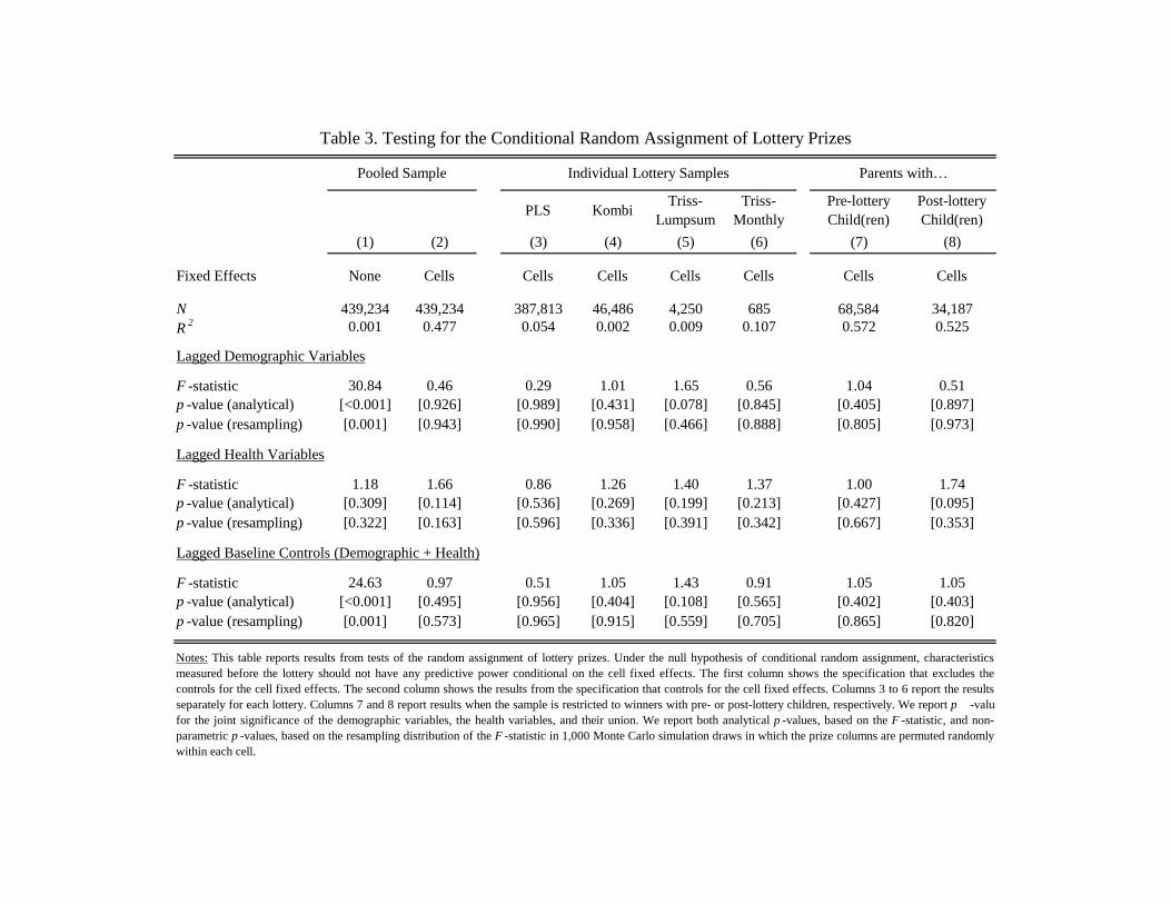
PLS Kombi Triss-Lumpsum

Triss-Monthly

Pre-lottery Child(ren)

Post-lottery Child(ren)

(1) (2) (3) (4) (5) (6) (7) (8)

Fixed Effects None Cells Cells Cells Cells Cells Cells Cells

N 439,234 439,234 387,813 46,486 4,250 685 68,584 34,187R 2 0.001 0.477 0.054 0.002 0.009 0.107 0.572 0.525

Lagged Demographic Variables

F -statistic 30.84 0.46 0.29 1.01 1.65 0.56 1.04 0.51p -value (analytical) [<0.001] [0.926] [0.989] [0.431] [0.078] [0.845] [0.405] [0.897]p -value (resampling) [0.001] [0.943] [0.990] [0.958] [0.466] [0.888] [0.805] [0.973]

Lagged Health Variables

F -statistic 1.18 1.66 0.86 1.26 1.40 1.37 1.00 1.74p -value (analytical) [0.309] [0.114] [0.536] [0.269] [0.199] [0.213] [0.427] [0.095]p -value (resampling) [0.322] [0.163] [0.596] [0.336] [0.391] [0.342] [0.667] [0.353]

Lagged Baseline Controls (Demographic + Health)

F -statistic 24.63 0.97 0.51 1.05 1.43 0.91 1.05 1.05p -value (analytical) [<0.001] [0.495] [0.956] [0.404] [0.108] [0.565] [0.402] [0.403]p -value (resampling) [0.001] [0.573] [0.965] [0.915] [0.559] [0.705] [0.865] [0.820]

Pooled Sample Individual Lottery Samples Parents with…

Notes: This table reports results from tests of the random assignment of lottery prizes. Under the null hypothesis of conditional random assignment, characteristicsmeasured before the lottery should not have any predictive power conditional on the cell fixed effects. The first column shows the specification that excludes thecontrols for the cell fixed effects. The second column shows the results from the specification that controls for the cell fixed effects. Columns 3 to 6 report the resultsseparately for each lottery. Columns 7 and 8 report results when the sample is restricted to winners with pre- or post-lottery children, respectively. We report p -value for the joint significance of the demographic variables, the health variables, and their union. We report both analytical p -values, based on the F -statistic, and non-parametric p -values, based on the resampling distribution of the F -statistic in 1,000 Monte Carlo simulation draws in which the prize columns are permuted randomlywithin each cell.

Table 3. Testing for the Conditional Random Assignment of Lottery Prizes

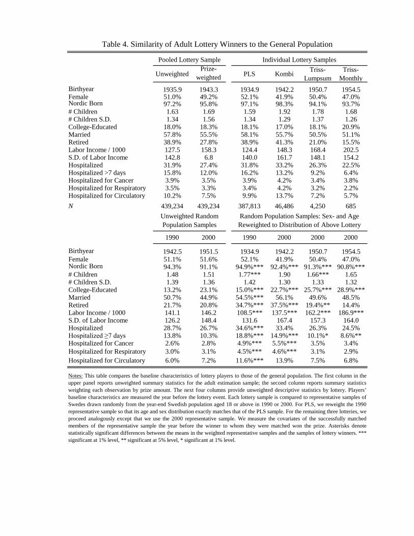
Unweighted Prize-

weighted PLS Kombi Triss-Lumpsum

Triss-Monthly

Birthyear 1935.9 1943.3 1934.9 1942.2 1950.7 1954.5Female 51.0% 49.2% 52.1% 41.9% 50.4% 47.0%Nordic Born 97.2% 95.8% 97.1% 98.3% 94.1% 93.7%# Children 1.63 1.69 1.59 1.92 1.78 1.68# Children S.D. 1.34 1.56 1.34 1.29 1.37 1.26College-Educated 18.0% 18.3% 18.1% 17.0% 18.1% 20.9%Married 57.8% 55.5% 58.1% 55.7% 50.5% 51.1%Retired 38.9% 27.8% 38.9% 41.3% 21.0% 15.5%Labor Income / 1000 127.5 158.3 124.4 148.3 168.4 202.5S.D. of Labor Income 142.8 6.8 140.0 161.7 148.1 154.2Hospitalized 31.9% 27.4% 31.8% 33.2% 26.3% 22.5%Hospitalized >7 days 15.8% 12.0% 16.2% 13.2% 9.2% 6.4%Hospitalized for Cancer 3.9% 3.5% 3.9% 4.2% 3.4% 3.8%Hospitalized for Respiratory 3.5% 3.3% 3.4% 4.2% 3.2% 2.2%Hospitalized for Circulatory 10.2% 7.5% 9.9% 13.7% 7.2% 5.7%N 439,234 439,234 387,813 46,486 4,250 685

1990 2000 1990 2000 2000 2000

Birthyear 1942.5 1951.5 1934.9 1942.2 1950.7 1954.5Female 51.1% 51.6% 52.1% 41.9% 50.4% 47.0%Nordic Born 94.3% 91.1% 94.9%*** 92.4%*** 91.3%*** 90.8%***# Children 1.48 1.51 1.77*** 1.90 1.66*** 1.65# Children S.D. 1.39 1.36 1.42 1.30 1.33 1.32College-Educated 13.2% 23.1% 15.0%*** 22.7%*** 25.7%*** 28.9%***Married 50.7% 44.9% 54.5%*** 56.1% 49.6% 48.5%Retired 21.7% 20.8% 34.7%*** 37.5%*** 19.4%** 14.4%Labor Income / 1000 141.1 146.2 108.5*** 137.5*** 162.2*** 186.9***S.D. of Labor Income 126.2 148.4 131.6 167.4 157.3 164.0Hospitalized 28.7% 26.7% 34.6%*** 33.4% 26.3% 24.5%Hospitalized ≥7 days 13.8% 10.3% 18.8%*** 14.9%*** 10.1%* 8.6%**Hospitalized for Cancer 2.6% 2.8% 4.9%*** 5.5%*** 3.5% 3.4%Hospitalized for Respiratory 3.0% 3.1% 4.5%*** 4.6%*** 3.1% 2.9%Hospitalized for Circulatory 6.0% 7.2% 11.6%*** 13.9% 7.5% 6.8%

Table 4. Similarity of Adult Lottery Winners to the General Population

Pooled Lottery Sample

Unweighted Random Population Samples

Random Population Samples: Sex- and Age Reweighted to Distribution of Above Lottery

Notes: This table compares the baseline characteristics of lottery players to those of the general population. The first column in theupper panel reports unweighted summary statistics for the adult estimation sample; the second column reports summary statisticsweighting each observation by prize amount. The next four columns provide unweighted descriptive statistics by lottery. Players’baseline characteristics are measured the year before the lottery event. Each lottery sample is compared to representative samples ofSwedes drawn randomly from the year-end Swedish population aged 18 or above in 1990 or 2000. For PLS, we reweight the 1990representative sample so that its age and sex distribution exactly matches that of the PLS sample. For the remaining three lotteries, weproceed analogously except that we use the 2000 representative sample. We measure the covariates of the successfully matchedmembers of the representative sample the year before the winner to whom they were matched won the prize. Asterisks denotestatistically significant differences between the means in the weighted representative samples and the samples of lottery winners. ***significant at 1% level, ** significant at 5% level, * significant at 1% level.

Individual Lottery Samples

PLS Kombi Triss-Lumpsum

Triss-Monthly

Less than 10K SEK 404,165 358,141 46,024 0 0 61,944 30,79610K to 100K SEK 27,109 25,926 0 1,183 0 5,053 2,827100K to 500K SEK 5,293 2,650 0 2,643 0 1,147 450500K to 1M SEK 527 324 0 203 0 68 32>1M SEK 2,140 772 462 221 685 372 82TOTAL 439,234 387,813 46,486 4,250 685 68,584 34,187

Notes: This table shows the number of prizes assigned to individuals in our final estimation sample. Non-winning controls in Kombi are included asprizes below 10K. All prizes are deflated by a consumer price index normalized to 1 in 2010. Monthly installments for Triss-Monthly have beenconverted to net present values using a 2 % real discount rate.

Table 5. Distribution of Prizes Awarded

Parents with Pre-Lottery Child(ren)

Parents with Post-Lottery Child(ren)

Adult Lottery Samples by LotteryAdult Sample

Pooled Lottery Age 45-69 Age 70+ (1) (2) (3) (5) (6)

Prize/Wealth (in 1M SEK) 1.015 0.874 0.828 0.963 1.054s.e. (0.026) (0.015) (0.015) (0.041) (0.036)p -value [0.564] [<0.001] [<0.001] [0.370] [0.127]Controls Baseline Baseline Birth Baseline Baseline# At Risk 439,234 49,959 49,959 220,271 130,225# Deaths 139,049 5,165 5,165 44,928 91,890

Female Male Yes No No Yes Below Above(7) (8) (9) (10) (11) (12) (13) (14)

Prize (in 1M SEK) 1.058 0.973 0.960 1.020 1.016 1.026 1.018 1.015s.e. (0.041) (0.035) (0.086) (0.027) (0.040) (0.036) (0.028) (0.066)p -value [0.147] [0.437] [0.647] [0.461] [0.691] [0.467] [0.506] [0.818]Controls Baseline Baseline Baseline Baseline Baseline Baseline Baseline Baseline# At Risk 224,083 215,151 78,869 360,365 299,037 140,197 219,655 219,579# Deaths 67,003 72,046 12,521 126,528 71,084 67,965 116,365 22,684

Table 6. Proportional Hazard Model Estimates of the Effect of Wealth on Mortality

Notes: This table shows the estimated hazard ratios from survival models with right censoring. Wealth is scaled so that a regression coefficient of 1.1 denotes a 10% increase in the hazard per million SEK(at 2010 prices). The reported sample size and number of deaths in the representative sample is given prior to reweighting. Standard errors are clustered by individual and are reported in parentheses, and p -values are in brackets.

Sex College Hospitalized Income > Median

Representative Sample Age 18-44(4)

0.920

[0.322]Baseline88,7382,231

(0.078)

Any >=7days Health Index

(1) (2) (3)

Effect on P(Hospitalized) 0.304 -0.132 -0.080s.e. (0.505) (0.343) (0.143)p -value (analytical) [0.547] [0.700] [0.577]p -value (resampling) [0.525] [0.741] [0.488]Proportion 25.6% 12.6% Mean 14.478N 415,215 415,215 S.D. 24.219

N 431,064

Effect on P(Hospitalized) 0.393 0.437 0.297s.e. (0.617) (0.474) (0.268)p -value (analytical) [0.524] [0.356] [0.267]p -value (resampling) [0.555] [0.364] [0.220]Proportion 38.3% 19.2% Mean 20.993N 378,099 378,099 S.D. 31.495

N 418,002

Effect on P(Hospitalized) -0.027 0.106 0.453s.e. (0.770) (0.654) (0.355)p -value (analytical) [0.972] [0.871] [0.202]p -value (resampling) [0.977] [0.863] [0.210]Proportion 51.2% 25.9% Mean 31.088N 296,904 296,904 S.D. 38.508

N 367,863

Table 7. The Effect of Wealth on Hospitalization

Notes: In the regressions shown in columns 1 and 2, wealth is scaled so that a regression coefficient of 1.00denotes a 1 percentage point increase in hospitalization per million SEK (at 2010 prices). Wealth is scaled inmillion SEK in regressions shown in column 3, and the outcome variable takes values between 0 and 100. Allregressions include controls for the baseline demographic and health variables described in the text. Standarderrors are clustered by individual and are reported in parentheses, and p -values are in brackets. We also reportnon-parametric p -values based on the resampling distribution of the estimated coefficient in 1,000 Monte Carlosimulation draws in which the prize columns are permuted randomly within each cell.

Panel A: Within 2 years after win

Panel B: Within 5 years after win

Panel C: Within 10 years after win

Hospitalizations

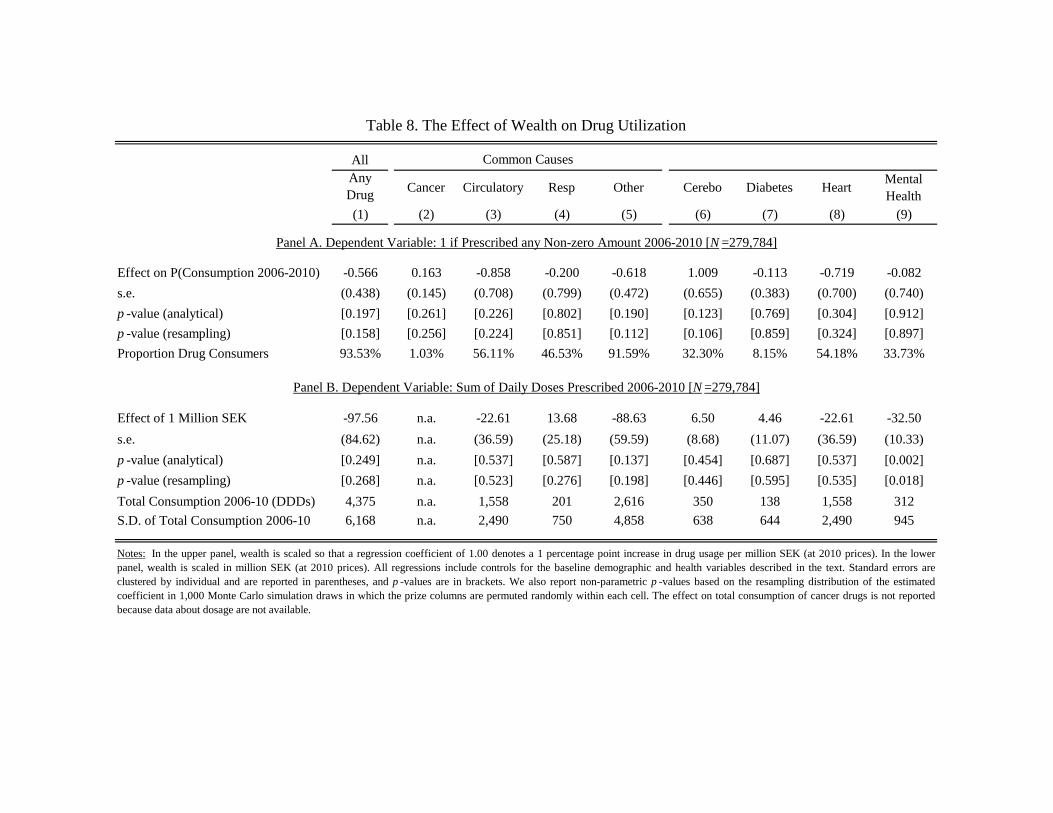
AllAnyDrug Cancer Circulatory Resp Other Cerebo Diabetes Heart Mental

Health (1) (2) (3) (4) (5) (6) (7) (8) (9)

Effect on P(Consumption 2006-2010) -0.566 0.163 -0.858 -0.200 -0.618 1.009 -0.113 -0.719 -0.082s.e. (0.438) (0.145) (0.708) (0.799) (0.472) (0.655) (0.383) (0.700) (0.740)p -value (analytical) [0.197] [0.261] [0.226] [0.802] [0.190] [0.123] [0.769] [0.304] [0.912]p -value (resampling) [0.158] [0.256] [0.224] [0.851] [0.112] [0.106] [0.859] [0.324] [0.897]Proportion Drug Consumers 93.53% 1.03% 56.11% 46.53% 91.59% 32.30% 8.15% 54.18% 33.73%

Effect of 1 Million SEK -97.56 n.a. -22.61 13.68 -88.63 6.50 4.46 -22.61 -32.50s.e. (84.62) n.a. (36.59) (25.18) (59.59) (8.68) (11.07) (36.59) (10.33)p -value (analytical) [0.249] n.a. [0.537] [0.587] [0.137] [0.454] [0.687] [0.537] [0.002]p -value (resampling) [0.268] n.a. [0.523] [0.276] [0.198] [0.446] [0.595] [0.535] [0.018]Total Consumption 2006-10 (DDDs) 4,375 n.a. 1,558 201 2,616 350 138 1,558 312S.D. of Total Consumption 2006-10 6,168 n.a. 2,490 750 4,858 638 644 2,490 945

Notes: In the upper panel, wealth is scaled so that a regression coefficient of 1.00 denotes a 1 percentage point increase in drug usage per million SEK (at 2010 prices). In the lowerpanel, wealth is scaled in million SEK (at 2010 prices). All regressions include controls for the baseline demographic and health variables described in the text. Standard errors areclustered by individual and are reported in parentheses, and p -values are in brackets. We also report non-parametric p -values based on the resampling distribution of the estimatedcoefficient in 1,000 Monte Carlo simulation draws in which the prize columns are permuted randomly within each cell. The effect on total consumption of cancer drugs is not reportedbecause data about dosage are not available.

Table 8. The Effect of Wealth on Drug Utilization

Common Causes

Panel A. Dependent Variable: 1 if Prescribed any Non-zero Amount 2006-2010 [N =279,784]

Panel B. Dependent Variable: Sum of Daily Doses Prescribed 2006-2010 [N =279,784]

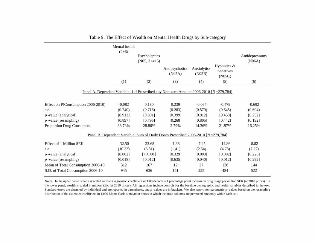
Mental health (2+6)

Psycholeptics (N05, 3+4+5)

Antidepressants (N06A)

Antipsychotics (N05A)

Anxiolytics (N05B)

Hypnotics & Sedatives (N05C)

(1) (2) (3) (4) (5) (6)

Effect on P(Consumption 2006-2010) -0.082 0.180 0.239 -0.064 -0.479 -0.692s.e. (0.740) (0.716) (0.283) (0.579) (0.645) (0.604)p -value (analytical) [0.912] [0.801] [0.399] [0.912] [0.458] [0.252]p -value (resampling) [0.897] [0.795] [0.268] [0.805] [0.442] [0.192]Proportion Drug Consumers 33.73% 28.86% 2.79% 14.36% 21.97% 16.25%

Effect of 1 Million SEK -32.50 -23.68 -1.38 -7.45 -14.86 -8.82s.e. (10.33) (6.31) (1.41) (2.54) (4.73) (7.27)p -value (analytical) [0.002] [<0.001] [0.329] [0.003] [0.002] [0.226]p -value (resampling) [0.018] [0.012] [0.635] [0.040] [0.012] [0.292]Mean of Total Consumption 2006-10 312 167 12 27 128 144S.D. of Total Consumption 2006-10 945 636 161 225 484 522

Panel B. Dependent Variable: Sum of Daily Doses Prescribed 2006-2010 [N =279,784]

Notes: In the upper panel, wealth is scaled so that a regression coefficient of 1.00 denotes a 1 percentage point increase in drug usage per million SEK (at 2010 prices). Inthe lower panel, wealth is scaled in million SEK (at 2010 prices). All regressions include controls for the baseline demographic and health variables described in the text.Standard errors are clustered by individual and are reported in parentheses, and p -values are in brackets. We also report non-parametric p -values based on the resamplingdistribution of the estimated coefficient in 1,000 Monte Carlo simulation draws in which the prize columns are permuted randomly within each cell.

Table 9. The Effect of Wealth on Mental Health Drugs by Sub-category

Panel A. Dependent Variable: 1 if Prescribed any Non-zero Amount 2006-2010 [N =279,784]

Pooled Mother Pooled Mother Pooled Mother(1) (2) (3) (4) (5) (6)

Effect of 1 M SEK -11.036 16.265 -0.647 -1.140 -1.289 -1.461s.e. (29.118) (42.802) (0.623) (1.162) (0.635) (0.741)p -value (analytical) [0.705] [0.704] [0.299] [0.327] [0.042] [0.049]p -value (re-sampling) [0.517] [0.815] [0.278] [0.723] [0.042] [0.128]Mean / Proportion 3,546.81 3,545.83 4.13% 4.00% 6.28% 5.91%S.D. 588.40 582.73N 54,575 24,977 54,575 24,977 54,695 25,026

t=2 t=5 t=2 t=5 t=2 t=5 t=2 t=5(7) (8) (9) (10) (11) (12) (13) (14)

Effect of 1 M SEK 2.119 3.443 0.400 0.227 0.864 0.949 0.320 1.017s.e. (0.747) (0.913) (0.291) (0.320) (0.519) (0.776) (0.381) (0.768)p -value (analytical) [0.005] [0.0002] [0.170] [0.478] [0.096] [0.222] [0.400] [0.185]p -value (re-sampling) [0.002] [<0.001] [0.142] [0.440] [0.018] [0.124] [0.388] [0.178]Proportion 10.89% 17.99% 1.70% 2.78% 2.76% 4.78% 2.66% 4.93%N 114,160 111,064 114,160 111,064 100,327 75,382 100,327 75,382

Total Mental Health

Allergy & Asthma ADHD BMI Over-

weight Obese

(15) (16) (17) (18) (19) (20) (21)Effect of 1 M SEK 8.895 -3.710 5.378 -11.247 -0.113 -0.919 -2.141s.e. (27.656) (12.463) (12.930) (7.645) (0.225) (2.324) (0.858)p -value (analytical) [0.748] [0.766] [0.677] [0.141] [0.614] [0.692] [0.013]p -value (resampling) [0.577] [0.909] [0.599] [0.502] [0.585] [0.695] [0.002]Mean / Proportion 468.34 105.51 91.45 13.45 22.40 15.87% 2.91%S.D. 1540.46 575.50 357.47 156.26 3.17N 112,223 105,197 21,298 20,656 32,646 32,646 32,646

Panel B: Hospitalizations

Panel C: Drug Prescription and BMI

Table 10. The Effect of Wealth on Pre-specified Child Health Outcomes

External

Notes: This table shows the estimated effect of wealth on child health. The effect of infant health is shown both for all post-lottery children and forchildren of female winners only. Hospitalizations refer to binary variables indicating whether the child was hospitalized within two or five years after thelottery draw. Consumption of prescribed drugs refers to the annual average number of daily doses prescribed in 2006-2010 multipled by 5. BMI ismeasured at conscription and is available for men only. Overweight refers to a BMI above 25, and obesity refers to a BMI above 30. Wealth is scaled sothat a marginal effect of 1.00 denotes a 1 percentage point increase per million SEK (at 2010 prices) for binary outcomes, whereas it is scaled in millionsof SEK for other outcomes. All regressions include controls for birth characteristics of the child and demographic controls for the winning parent.Standard errors are clustered by extended family and are reported in parentheses, and p -values are in brackets. We also report non-parametric p -values based on the resampling distribution of the estimated coefficient in 1,000 Monte Carlo simulation draws in which the prize columns are permutedrandomly within each cell.

All Causes All causes > 7 days Respiratory

Panel A: Infant Health

Low Birthweight (< 2500 grams)

Birthweight(in grams)

Premature Birth(< 37 weeks)

Swedish English Math

(1) (2) (3) (4) (5) (6)

Effect of 1 Million SEK -0.113 -0.031 -0.022 -0.034 -0.081 -0.029s.e. (0.048) (0.077) (0.027) (0.039) (0.043) (0.052)p -value (analytical) [0.019] [0.686] [0.424] [0.385] [0.060] [0.579]p -value (resampling) [0.074] [0.573] [0.679] [0.478] [0.172] [0.611]Mean 0.169 0.143 0.271 0.163 0.105 0.204S.D. 0.976 0.976 0.938 0.996 0.990 1.013N 36,435 31,550 74,187 25,079 25,286 23,990

Table 11. The Effect of Wealth on Pre-specified Child Skills

Notes: This table shows the estimated effect of wealth on child skills. Cognitive and non-cognitive skills are measured at conscriptionand are available for men only. GPA refers to the grade point average in ninth grade. The outcome variable in columns 4 to 6 refers tothe score on national tests taken in ninth grade. All outcome variables are standardized so that the mean in the full population is 1 andstandard deviation is 1. Coefficients are scaled so that a coefficient of 1.00 denotes a 1 standard deviation increase in skills permillion SEK won (at 2010 prices). All regressions include controls for birth characteristics of the child and demographic controls forthe winning parent. Standard errors are clustered by extended family and are reported in parentheses, and p -values are in brackets.We also report non-parametric p -values based on the resampling distribution of the estimated coefficient in 1,000 Monte Carlosimulation draws in which the prize columns are permuted randomly within each cell.

Cognitive skills

Non-cognitive

skillsGPA

National Test Scores

Mother Father

(1) (2) (3) (4) (5) (6) (7)Effect of 1 M SEK 0.006 -0.009 -35.526 -30.661 -18.466 5.411 -0.953s.e. (0.007) (0.011) (15.833) (13.913) (15.880) (8.361) (1.040)p -value (analytical) [0.399] [0.394] [0.025] [0.028] [0.245] [0.518] [0.359]p -value (resampling) [0.342] [0.470] [0.092] [0.126] [0.178] [0.250] [0.262]Mean / Proportion 0.08 0.02 389.61 224.02 385.99 79.79 6.93%S.D. 0.18 0.27 1002.49 868.67 177.82 119.80N 36,982 74,459 147,969 131,815 9,868 11,750 51,753Unit of analysis Child Child Winner Winner Child Child Child

Notes: This table shows the estimated effect of wealth on different proxies for parental investments. Column 1 shows the effect on childwealth five years after the lottery draw. Wealth is measured in million SEK (at 2010 prices) and winsorized at the 99th percentile. Schoolquality refers to the average GPA in the school in which the child finished ninth grade. Mental health drug consumption is the total numberof daily doses consumed between 2006 and 2010. Maternal/paternal leave is measured in number of days of paid parental leave. Smokingduring pregnancy is an indicator variable indicating whether the mother reported having smoked during pregnancy. Lottery wealth is scaledin million SEK (at 2010) prices in columns 1 to 6. The coefficient for mother's smoking in column 7 is scaled so that a regression coefficientof 1.00 denotes a 1 percentage point increase per million SEK. All regressions include controls for birth characteristics of the child anddemographic controls for the winning parent. Standard errors are clustered by extended family in all regressions in which children is the unitof analysis, and by individual for parental mental health. We also report non-parametric p -values based on the resampling distribution of theestimated coefficient in 1,000 Monte Carlo simulation draws in which the prize columns are permuted randomly within each cell.

Pre-lottery Children Post-lottery Children

Table 12. Proxies for Parental Investment

Mental Health Drugs Smoking during

Pregnancy

Paternal Leave

Maternal Leave

School QualityWealth