ARTICLEReceived 15 Jan 2014 | Accepted 9 Jul 2014 | Published 2 Sep 2014

Weakening of the stratospheric polarvortex by Arctic sea-ice lossBaek-Min Kim1, Seok-Woo Son2, Seung-Ki Min3, Jee-Hoon Jeong4, Seong-Joong Kim1, Xiangdong Zhang5,

Taehyoun Shim4 & Jin-Ho Yoon6

Successive cold winters of severely low temperatures in recent years have had critical social

and economic impacts on the mid-latitude continents in the Northern Hemisphere. Although

these cold winters are thought to be partly driven by dramatic losses of Arctic sea-ice, the

mechanism that links sea-ice loss to cold winters remains a subject of debate. Here, by

conducting observational analyses and model experiments, we show how Arctic sea-ice

loss and cold winters in extra-polar regions are dynamically connected through the polar

stratosphere. We find that decreased sea-ice cover during early winter months (November–

December), especially over the Barents–Kara seas, enhances the upward propagation of

planetary-scale waves with wavenumbers of 1 and 2, subsequently weakening the strato-

spheric polar vortex in mid-winter (January–February). The weakened polar vortex

preferentially induces a negative phase of Arctic Oscillation at the surface, resulting in low

temperatures in mid-latitudes.

DOI: 10.1038/ncomms5646

1 Division of Polar Climate Change Research, Korea Polar Research Institute, Incheon 406-840, Korea. 2 School of Earth and Environmental Sciences, SeoulNational University, Seoul 151-742, Korea. 3 School of Environmental Science and Engineering, Pohang University of Science and Technology, Pohang 790-784,Korea. 4 Department of Oceanography, Chonnam National University, Gwangju 500-757, Korea. 5 International Arctic Research Center and Department ofAtmospheric Sciences, University of Alaska, Fairbanks, Alaska 99775, USA. 6 Pacific Northwest National Laboratory, Richland, Washington 99352, USA.Correspondence and requests for materials should be addressed to S.-J.K. (email: seongjkim@kopri.re.kr).

NATURE COMMUNICATIONS | 5:4646 | DOI: 10.1038/ncomms5646 | www.nature.com/naturecommunications 1

& 2014 Macmillan Publishers Limited. All rights reserved.

Over the past two decades, the Arctic Ocean has warmedsignificantly in conjunction with conspicuous increase inglobal surface air temperature (SAT) and rapid decline of

Arctic sea-ice1,2. A growing number of studies have foundpronounced changes in atmospheric circulation due to Arctic sea-ice loss, including changes in the tropospheric jet stream that maylead to cold extremes over Eurasia and North America3–7.However, because the occurrence of major sea-ice losses has beenrelatively recent, a robust connection between Arctic sea-ice andatmospheric circulation has not been well-established, and theunderlying mechanism(s) responsible for these processes are notyet fully understood8,9. For example, through the analysis of re-analysis data and climate model outputs, a number of studieshave suggested that Arctic sea-ice loss has the potential to forcethe Arctic Oscillation (AO) into its negative phase10–12. Incontrast, other recent studies have emphasized the impact ofplanetary-scale wave pattern over the Eurasian continent thatemanates from the Barents–Kara (B–K) seas4,13,14. Apparently,this pattern appears to be zonally asymmetric and different froma typical pattern of the AO15.

Efforts have also been made to relate the recent changes incryospheric conditions such as Eurasian snow cover and Arctic sea-ice cover to the variability of the stratospheric polar vortex16–18. Itis documented that the variability of the stratospheric polar vortexhas increased in recent years. For instance, whereas the suddenweakening of the stratospheric polar vortex, known as a majorSudden Stratospheric Warming (SSW) event, occurred relativelyinfrequently during the 1990s according to the WorldMeteorological Organization (WMO) definition of SSW19, it hasoccurred almost every year since 2000 (ref. 20). SSW events areoften followed by a negative phase of the AO at the surface with atime lag of 1 or 2 months21–23. This indicates that understandingpossible contributors to recent stratospheric variability, which mayinclude cryospheric changes24, is critical for the betterunderstanding of the surface climate variability in the recent past.

A systematic study that considers both bottom-up and top-down processes occurring within the cryosphere, troposphere andstratosphere is therefore crucial for elucidating how Arctic sea-iceinteracts with atmospheric circulation and thereby causes extremesurface weather events. In this study, a time-lagged stratosphericresponse to Arctic sea-ice loss is examined via composite analyses

that utilize both European Center for Medium-RangeWeather Forecasts (ECMWF) Re-Analysis Interim (ERA-Interim) data25 and climate model sensitivity experiments. Thissynthetic analysis reveals that polar stratospheric variability ispartly controlled by marked losses of Arctic sea-ice, especiallyover the B–K seas.

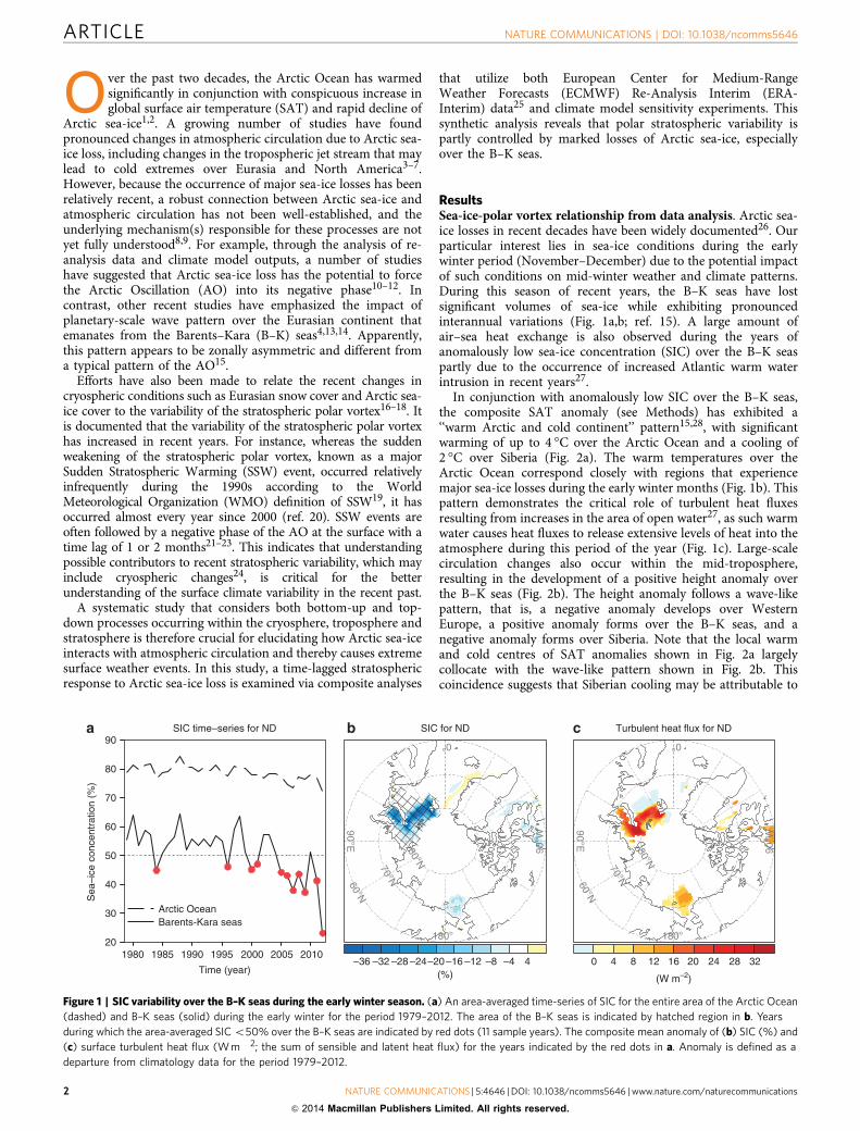
ResultsSea-ice-polar vortex relationship from data analysis. Arctic sea-ice losses in recent decades have been widely documented26. Ourparticular interest lies in sea-ice conditions during the earlywinter period (November–December) due to the potential impactof such conditions on mid-winter weather and climate patterns.During this season of recent years, the B–K seas have lostsignificant volumes of sea-ice while exhibiting pronouncedinterannual variations (Fig. 1a,b; ref. 15). A large amount ofair–sea heat exchange is also observed during the years ofanomalously low sea-ice concentration (SIC) over the B–K seaspartly due to the occurrence of increased Atlantic warm waterintrusion in recent years27.

In conjunction with anomalously low SIC over the B–K seas,the composite SAT anomaly (see Methods) has exhibited a‘‘warm Arctic and cold continent’’ pattern15,28, with significantwarming of up to 4 !C over the Arctic Ocean and a cooling of2 !C over Siberia (Fig. 2a). The warm temperatures over theArctic Ocean correspond closely with regions that experiencemajor sea-ice losses during the early winter months (Fig. 1b). Thispattern demonstrates the critical role of turbulent heat fluxesresulting from increases in the area of open water27, as such warmwater causes heat fluxes to release extensive levels of heat into theatmosphere during this period of the year (Fig. 1c). Large-scalecirculation changes also occur within the mid-troposphere,resulting in the development of a positive height anomaly overthe B–K seas (Fig. 2b). The height anomaly follows a wave-likepattern, that is, a negative anomaly develops over WesternEurope, a positive anomaly forms over the B–K seas, and anegative anomaly forms over Siberia. Note that the local warmand cold centres of SAT anomalies shown in Fig. 2a largelycollocate with the wave-like pattern shown in Fig. 2b. Thiscoincidence suggests that Siberian cooling may be attributable to

90a b cSIC time–series for ND SIC for ND Turbulent heat flux for ND

80

70

60

50

40

Sea

–ice

con

cent

ratio

n (%

)

30

201980 1985 1990

Arctic OceanBarents-Kara seas

1995

Time (year)

2000 2005 2010–36 –32 –28 –24

180°

0°

60°N

70°N

80°N

–20–16 –12 –8 –4 0 4 8 12 16 20 24 28 32

(W m–2)

4(%)

90°E

90°W

180°

0°

60°N

70°N

80°N

90°E

90°W

Figure 1 | SIC variability over the B–K seas during the early winter season. (a) An area-averaged time-series of SIC for the entire area of the Arctic Ocean(dashed) and B–K seas (solid) during the early winter for the period 1979–2012. The area of the B–K seas is indicated by hatched region in b. Yearsduring which the area-averaged SIC o50% over the B–K seas are indicated by red dots (11 sample years). The composite mean anomaly of (b) SIC (%) and(c) surface turbulent heat flux (W m! 2; the sum of sensible and latent heat flux) for the years indicated by the red dots in a. Anomaly is defined as adeparture from climatology data for the period 1979–2012.

ARTICLE NATURE COMMUNICATIONS | DOI: 10.1038/ncomms5646

2 NATURE COMMUNICATIONS | 5:4646 | DOI: 10.1038/ncomms5646 | www.nature.com/naturecommunications

& 2014 Macmillan Publishers Limited. All rights reserved.

the development of a planetary-scale wave train that is induced bysea-ice loss in the B–K seas.

Polar vortex variability can be readily assessed using the polarcap height (PCH) anomaly, which is obtained from the area-averaged geopotential height anomaly over the area north of65!N, normalized by the standard deviation for each of thestandard 26 pressure levels29. By definition, the existence of apositive PCH anomaly corresponds to a weakened polar vortexand can be related to the negative phase of the Northern AnnularMode. The surface PCH anomaly is linearly correlated with theAO index29.

To identify the linkage between the sea-ice and the strato-spheric polar vortex variability, a composite analysis is conductedas a function of time and pressure (Fig. 2c). Figure 2c shows theseasonal evolution of the composite PCH anomaly for the years ofanomalously low SIC over the B–K seas. The positive PCHanomaly dominates for the majority of winters, indicating aweakening of the polar vortex. However, the behaviour of thepolar vortex during early winter differs from that in mid-winter

(January–February). During early winter, the positive PCHanomaly remains largely confined to the troposphere and tendsto be relatively weaker in magnitude than during mid-winter. Thepattern depicted in Fig. 2b, which is asymmetric in the zonaldirection, contributes to the development of a positive PCHtropospheric anomaly during the early winter months. Incontrast, beginning in early January, a positive PCH anomalyappears in the upper stratosphere that descends thereafter,indicating the possible dynamic coupling between the strato-sphere and troposphere. In the later section, we will show thatthis weakening of the stratospheric polar vortex in early Januarycan be explained by the increased poleward heat flux anomalies at100 hPa (Fig. 2d), which is the indicator of the vertical flux ofwave activity from the troposphere.

Modelling evidence. The statistical analysis described above sug-gests that the development of a weakened mid-winter polar vortexin recent years may be attributed to the occurrence of sea-ice loss

a ∆SAT for ND, composite b ∆Z500 for ND, composite

c ∆PCH, composite

180°

0°

90°W

30°N

10

20

50

100

200

Pre

ssur

e (h

Pa)

500

1,000

6

3

0

–3

1 NOV 16 NOV

0.30.3

0.6

0.6

0.9

1.20.6

0.9

–1.5 –24–20–16–12–8–4

4812162024283236

(gpm)

–1.2–0.9

–0.6

0.6

0.6

0.6

1.8

1.2

0.6

1.2–0.6

–1.2

–0.6

–0.30.30.60.91.2

1.5

1.82.12.4

2.7

(°C)

0.3

0.3

0.6

1 DEC 16 DEC 1 JAN 16 JANTime (day)

1 FEB 16 FEB 1 MAR 16 MAR

–0.9

–0.6

–0.3

0.3

0.6

0.9

1.2

d

1 NOV 16 NOV 1 DEC 16 DEC 1 JAN 16 JANTime (day)

1 FEB 16 FEB 1 MAR 16 MAR

∆[v′T′], composite

[v′T

′] (°

C m

s–1

)

90°E

180°

0°

90°W

30°N

45°N

60°N

90°E

45°N

60°N

168

–8

24

24

8

–16

75°N

Figure 2 | Composite mean differences during the years of reduced Arctic sea-ice. Composite mean differences from climatology data with respectto (a) surface air temperature, (b) the geopotential height anomaly at 500 hPa for the early winter, (c) the subseasonal evolution of the PCH as afunction of pressure and (d) 5-day averaged composite poleward heat flux anomalies at 100 hPa from ERA-Interim data. In a and b, contour intervals are0.3 !C and 4 m, respectively. In c, the contour interval is 0.3. Values that are statistically significant at the 95% confidence level are enclosed bya dotted line (see Methods).

NATURE COMMUNICATIONS | DOI: 10.1038/ncomms5646 ARTICLE

NATURE COMMUNICATIONS | 5:4646 | DOI: 10.1038/ncomms5646 | www.nature.com/naturecommunications 3

& 2014 Macmillan Publishers Limited. All rights reserved.

in the B–K seas. However, the robustness of the suggested rela-tionship must be tested further as the analyzed relationships mayhave resulted due to chance given the small number of years usedin the composite (11 years, indicated by red dots in Fig. 1a).

To support our findings, climate model experiments wereperformed using the Community Atmospheric Model Version 5(CAM5), which is a newly developed, state-of-the-art climatemodel30,31. Two experiments, that is, control and sea-iceperturbed runs, were prepared (see Methods). They only differin surface boundary conditions over the Arctic Ocean. Eachexperiment was composed of 40 independent runs of varyinginitial conditions to estimate ensemble-mean model responses.The modelled atmospheric response to sea-ice loss over the B–Kseas is then defined as the difference between the ensemble meanof the perturbed runs and that of the control runs. For furtherdetails, see the Methods section.

The modelled response successfully reproduces the overallresponse of the SAT and mid-tropospheric circulation to theanomalously low SIC over the B–K seas (compare Fig. 2a,b, andFig. 3a,b). In particular, similarities in the mid-tropospheric height

anomalies over the Eurasian continent confirm that sea-ice loss overthe B–K seas induces a planetary-scale wave train and contributes toEurasian surface cooling. However, differences are also foundbetween the modelled responses and composite anomaliesespecially over North America (Fig. 3a,b). These differences arelikely attributable to the fact that the surface boundary condition inthe model experiments is fixed everywhere except for the ArcticOcean which is not the case in the composite analysis.

In spite of this regional discrepancy, the modelled responsecaptures a significant weakening of mid-winter polar vortex in thestratosphere (Fig. 3c) as in composite analysis (Fig. 2c). Moreimportantly, the downward coupling between the stratosphereand troposphere occurring in late January and early February iseffectively reproduced. The resulting tropospheric circulationanomaly then favors cold surface temperatures over NorthernHemisphere continents in late winter (January–March)(Supplementary Fig. 1).

Identical model experiments were also performed using CAM3,the previous version of CAM5 (Supplementary Fig. 2). Despitesignificant differences in model physics and mean biases31,

a

c

∆SAT for ND, CAM5

∆PCH, CAM5

180°

0°

30°N

45°N

60°N75°N

d ∆[v′T′], CAM5

10

20

50

100

200

Pre

ssur

e (h

Pa)

500

1,000

6

3

0

–3

1 NOV 16 NOV 1 DEC 16 DEC

0.30.3 0.3

0.3 0.3

0.6

0.6

1 JAN 16 JANTime (day)

1 FEB 16 FEB 16 MAR1 MAR

1 NOV 16 NOV 1 DEC 16 DEC 1 JAN 16 JANTime (day)

1 FEB 16 FEB 16 MAR1 MAR

2.7

(°C) (gpm)

3632282420161284

–4–8–12–16–20–24

1.2

0.9

0.6

0.3

–0.3

–0.6

–0.9

2.42.11.81.51.20.90.60.3

–0.3–0.6–0.9–1.2–1.5

b ∆Z500 for ND, CAM5

[v′T

′] (°

C m

s–1

)

90°E

90°W

180°

0°

30°N

45°N

60°N75°N

90°E

90°W

Figure 3 | Model ensemble-mean responses for the reduced Arctic sea-ice condition. Model ensemble-mean responses to the reduced SIC over B–Kseas for (a) surface air temperature, (b) the geopotential height anomaly at 500 hPa for the early winter, (c) the subseasonal evolution of the PCHas a function of pressure and (d) 5-day averaged poleward heat flux anomalies at 100 hPa. In a and b, contour intervals are 0.3 !C and 4 m, respectively.In c, the contour interval is 0.3. Values that are statistically significant at the 95% confidence level are displayed by a dotted line (see Methods).

ARTICLE NATURE COMMUNICATIONS | DOI: 10.1038/ncomms5646

4 NATURE COMMUNICATIONS | 5:4646 | DOI: 10.1038/ncomms5646 | www.nature.com/naturecommunications

& 2014 Macmillan Publishers Limited. All rights reserved.

CAM3 experiments show essentially the same results to theCAM5 experiments. Although this consistency suggests that themodelling results may not be sensitive to the model physics andbias, further experiments using different models are needed toincrease the robustness of our findings.

Given the successful simulation of sea-ice-polar vortexrelationships (Fig. 3c), it is worthwhile to examine whethernoticeable differences in stratospheric variability exist betweenthe two model experiments. Specifically, we count SSW eventssimulated by the control and perturbed runs. A widely useddefinition of SSW event, zonal mean zonal wind reversal at 60!Nand 10 hPa, is employed here32. Out of the 40 ensemble membersof the control and perturbed experiments, a total of 17 and 25SSW events, or 0.35 and 0.64 events per year, were identified,respectively. This result is consistent with the more frequentoccurrence of SSW events during the years exhibiting lower SICover the B–K seas in the re-analysis data.

The consistency was also found in the overall polar vortexvariability, which was quantified from the frequency distributionof zonal mean zonal wind at 60!N at 10 hPa. Re-analysis datashows a slight increase in the frequency of weakened zonal windsduring the years with low SIC (Fig. 4a), although insufficientsample size introduces uncertainty. Model experiments produceessentially the same results to the composite analysis with morevisible frequency shifts toward the weaker winds (Fig. 4b). Theseresults suggest that sea-ice loss over the B–K seas generallyinduces more frequent occurrence of weak vortex events.

Upward wave propagation excited by Arctic sea-ice loss. Basedon the evidence derived from the statistical analysis of theobservation-based dataset and numerical modelling results, aphysical mechanism that explains the effect of Arctic sea-ice losson the stratospheric polar vortex was investigated. We hypothe-sized that the positive stratospheric PCH anomaly is driven byArctic sea-ice loss primarily through the vertical flux of waveactivity from the troposphere.

To test this hypothesis, we calculated the zonal-mean eddy heatflux, [v0T0], at 100 hPa averaged between 45!N and 75!N fromboth re-analysis and the model datasets33. Here, v is themeridional wind and T is the temperature at 100 hPa. Thebracket and prime denote the zonal mean and the deviation fromthe zonal mean, respectively. This quantity has been widely usedto quantify the intensity of vertically propagating wave activity.The composite [v0T0] anomaly using the re-analysis is shown inFig. 2d and the ensemble-mean response of [v0T0] obtained by themodel experiments is shown in Fig. 3d. Both demonstrate anemergence and gradual increase of vertical wave activity

preceding the occurrence of the positive stratospheric PCHanomaly33. Notable wave activity begins in early winter from thelower troposphere and then extends to the stratosphere by themid-winter months, accompanied by a dramatic increase inmagnitude. This time evolution suggests that sea-ice reductionsenhance vertical wave activity, which in turn produces a positivePCH anomaly or weak vortex in the stratosphere.

Further analyses reveal that the tropospheric wave disturbanceshown in Fig. 2b (Fig. 3b for the model response) is the maindriver of the enhanced vertical wave propagation during the earlywinter season. According to the quasi-geostrophic lineardynamics, vertically propagating waves should have zonaldisturbances that are tilted westward with heights34. Thiswestward tilting is observed in a wide range of waves rangingfrom synoptic to planetary scales. However, it is well-recognizedthat wavenumber 1 and 2 disturbances are the predominantwaves that propagate into the winter stratosphere andsubsequently weakening the polar vortex34.

To examine the horizontal and vertical structures of sea-ice-induced planetary-scale waves that propagate into the strato-sphere, the wave disturbance patterns depicted in Fig. 2b (Fig. 3bfor model response) are decomposed by wavenumber using aFourier transformation along the latitude circle. Figure 5apresents the zonal wavenumber 1 component for the geopotentialheight field at 300 hPa. The zonal and vertical structure averagedover 45!N-75!N is also provided for the zonal wavenumber 1component (Fig. 5c). The composite anomaly for the years withreduced sea-ice (contour) is compared with the long-termclimatology value (shading). Similarly, the ensemble-meanresponse of the geopotential height field is compared with thecontrol experiment mean (Fig. 5b,d). From these figures, thezonal and vertical structures of the zonal wavenumber 1anomalies are approximately in phase with the long-termclimatology for both the composite analysis and model simula-tions. Because wave energy is proportional to the square of waveamplitude, the wave that is in phase with climatological waveconstructively interferes with it. This constructive interferencealso occurs in zonal wavenumber 2 at a weaker magnitude.

In the Arctic Ocean, the model response and compositeanalysis show notable differences in wavenumber 1 component.However, the vertical wave activity that controls the stratosphereis not sensitive to the circulation anomaly over the Arctic Ocean,where the climatological stationary wave is almost absent. Notethat the vertical wave activity is, instead, determined by the eddyheat flux anomaly in mid-latitudes33.

According to recent studies35–37, the linear interference ofwavenumbers 1 and 2 largely determines the vertical wave activity

PDF of 10 hPa zonal winda

–40 –20 0 20 40 60 80U (ms–1) U (ms–1)

0.00

0.02

0.04

0.06

0.08

0.10

0.12

0.14

Den

sity

TotalB/K SIC < 50%

PDF of 10 hPa zonal windb

–40 –20 0 20 40 60 800.00

0.02

0.04

0.06

0.08

0.10

0.12

0.14

Den

sity

CAM5_ctrlCAM5_perturbed

Figure 4 | Histogram summary of stratospheric variability. (a) The normalized frequency distribution of daily zonal mean zonal wind at 60!Nat 10 hPa during the late winter for the period 1979–2012 (yellow) and for 11 years exhibiting SIC levels over the B–K seas that are o50% during earlywinter (green). (b) Same with a except for the model control experiment (yellow) and sea-ice perturbed experiment (green). In both figures, thesolid line indicates a five-point histogram value average. Note that the two distributions in both a and b overlap each other significantly. The overlappedregion is visualized by different colour (light green).

NATURE COMMUNICATIONS | DOI: 10.1038/ncomms5646 ARTICLE

NATURE COMMUNICATIONS | 5:4646 | DOI: 10.1038/ncomms5646 | www.nature.com/naturecommunications 5

& 2014 Macmillan Publishers Limited. All rights reserved.

of planetary-scale waves (see also Supplementary Fig. 3).Therefore, the result shown in Fig. 5 suggests that Arctic sea-ice anomalies tend to enhance vertically propagating planetary-scale waves by constructively interfering with climatologicalplanetary-scale waves, which likely weakens the polar vortex.

Upward wave propagation from the troposphere to thestratosphere has also been examined in the context of blockinghighs in the troposphere. It has been argued that the occurrenceof blocking at particular geographical locations, such as the B–Kseas and Ural Mountain regions, can cause vertically propagatingplanetary-scale waves; therefore, the occurrence of blocking canbe regarded as a tropospheric precursor to the stratospheric polarvortex weakening36,38,39. The present study supports this idea.Despite the regional differences, both the re-analysis andmodelling datasets demonstrate that regional blocking near theB–K seas tends to occur more frequently and persist for muchlonger periods in low sea-ice conditions over the B–K seas(Supplementary Fig. 4). This finding provides further evidence ofArctic sea-ice-related stratospheric changes.

DiscussionThrough a combination of observation-based data analysis andclimate model experiments, we provide corroborative evidencefor the notion that Arctic sea-ice loss over the B–K seas plays an

important role in weakening the stratospheric polar vortex.Regional sea-ice reductions over the B–K seas cause not onlyin situ surface warming but also significant upper-level responsesthat exhibit positive geopotential height anomalies over EasternEurope and negative anomalies from East Asia to the EasternPacific along the wave-guide of the tropospheric westerly jet. Thisanomaly pattern projects heavily into the climatological wave,intensifying the vertical propagation of planetary-scale wave intothe stratosphere and, in turn, weakening the stratospheric polarvortex. Therefore, planetary-scale wave generation by sea-icelosses and its upward propagation during early winter monthsunderline the link between surface climate variability and polarstratospheric variability.

The weakened stratospheric polar vortex is often followed by anegative phase of the AO at the surface21–23, favoring cold surfacetemperatures across Northern Hemisphere continents during thelate winter months (Supplementary Fig. 1). Several physicalmechanisms for this downward coupling have been proposed.They include the balanced response of the troposphere tostratospheric potential vorticity anomalies and wave-drivenchanges in the meridional circulation40,41. It is also suggestedthat the tropospheric response involves changes in the synopticeddies42,43. However, it has been difficult to isolate the keyprocess, and the detailed nonlinear processes involved are stillunder investigation21.

Wave-1 GPH at 300 hPa Wave-1 GPH at 300 hPaa

Z cross-section (composite)30

50

100

200

300

500

Pre

ssur

e (h

Pa)

700

1,000180 90W

–3

9

6

3

–9

0

Longitude (°)

90E 180

30

50

100

200

300

500

Pre

ssur

e (h

Pa)

700

1,000180 90W 0

Longitude (°)

90E 180

–200

–150

–100

–50

50

100

150

200

–200

–150

–100

–50

50

100

150

200

c Z Cross-section (model)d

125

100

75

50

–50

–75

–100

–125

ND composite ND model

5

10–10–5

10

510

15

–15–10

–5

180°

0°

30°N

45°N

60°N

75°N

b

125

100

75

50

–50

–75

–100

–125

90°E

90°W

180°

0°

30°N

45°N

60°N

75°N

90°E

90°W

–10–5

5

–5

5

10–5

6 –6

Figure 5 | Wavenumber 1 disturbance linked to Arctic sea-ice loss. (a) The zonal wavenumber 1 component of geopotential height at 300 hPa derivedfrom ERA-Interim data. The composite anomaly (contour) from the selected years of reduced Arctic sea-ice levels (red dots in Fig. 1a) is comparedwith the long-term climatology data (shading). (b) Same as a except for the model ensemble response (contour) and model climatology for thecontrol simulation (shading). Contour and shading intervals are 5 m and 25 m, respectively. (c) and (d): Same as a and b with the exception of thelongitude-pressure section averaged over 45!N–75!N. Contour and shading intervals are 3 m and 50 m, respectively.

ARTICLE NATURE COMMUNICATIONS | DOI: 10.1038/ncomms5646

6 NATURE COMMUNICATIONS | 5:4646 | DOI: 10.1038/ncomms5646 | www.nature.com/naturecommunications

& 2014 Macmillan Publishers Limited. All rights reserved.

As a final remark, we note that Arctic sea-ice loss representsonly one of the possible factors that can affect the stratosphericpolar vortex. Other factors reported in previous works includeEurasian snow cover, the Quasi Biannual Oscillation, the El-Ninoand Southern Oscillation and solar activity24,44,45. Systematicconsideration of these factors would extend our understanding ofclimate variability, possibly leading to the improved seasonalforecast46. Nonetheless, the relative contributions of each factorhave not been systematically examined. As these factors may beinterrelated, they may not control the stratospheric polar vortexindependently. These issues must be examined further in futureworks.

MethodsComposite analysis. SIC and Sea Surface Temperature (SST) are obtained fromHadley Centre Sea-Ice and SST data47. Eleven of the 34 years (1979–2012) duringwhich the averaged SIC over the B–K seas shows an anomalously low fraction(o50%; red dots in Fig. 1a) were selected for the composite analysis. Variousmeteorological fields including surface fluxes were obtained from ERA-Interim25

and analyzed at a spatial resolution of 1.5 by 1.5 degrees. Surface turbulent heatfluxes in Fig. 1c were computed by combining sensible and latent heat fluxes, whichare obtained from the ERA-Interim data.

Model configuration and experimental design. The CAM5 model was config-ured by a finite volume dynamical core with a horizontal resolution of 2.5!(longitude) by 1.9! (latitude) and 30 vertical levels extending to 3 hPa (B40 km).

A common challenge faced in the process of Arctic climate simulation isthe excessive wintertime low-level cloud in the model under extremely cold anddry conditions48,49. To reduce this bias, the model experiments in this studyapplied a modified formula for calculating fractions of low-level stratiform clouds(where air pressure levels X750 hPa). A detailed description of the formula isprovided in ref. 48.

Two sets of experiments were performed: that is, control and perturbed runs.The control experiment was conducted with a seasonal cycle of SIC and SST basedon the climatology of the Hadley Centre SIC and SST for the period 1979–2012(ref. 47). For the perturbed experiment, we introduced the composite seasonal cycleof SIC and SST to the Arctic Ocean during the years of reduced sea-ice, as indicatedin Fig. 1a (Supplementary Fig. 5). In this study, the Arctic Ocean is defined as thecollection of grid points in which the SIC value is 415% within the Arctic Circle(north of 65!N) at least once during the period 1979–2012. For the regions outsideof the Arctic Ocean, the same climatological SST condition that was used for thecontrol simulation was applied for the perturbed runs.

To obtain reliable model responses to the imposed sea-ice losses, both controland perturbed runs were conducted with 40 ensemble members by slightly varyingatmospheric initial conditions. Each integration started on 1 April and terminatedon 31 March, marking one full year of integration. The modelled atmosphericresponse is then defined as the ensemble-mean difference generated by subtractingthe ensemble-mean values of the perturbed runs from those of the control runs.

Statistical significance. The statistical significance of the composite meandifference and model ensemble-mean difference shown in Figs 2 and 3 wasdetermined by following a bootstrap resampling procedure by random samplingwith the replacement of 10,000 samples. Because we applied the statistical test foreach spatial grid point, we did not account the persistence in the time domain.Therefore, the area of statistical significance shown in Figs 2c and 3c (enclosed bythe dotted line) may be an underestimated value.

References1. Carmack, E. & Melling, H. Warmth from the deep. Nat. Geosci. 4, 7–8 (2011).2. Screen, J. A. & Simmonds, I. The central role of diminishing sea ice in recent

Arctic temperature amplification. Nature 464, 1334–1337 (2010).3. Jaiser, R., Dethloff, K., Handorf, D., Rinke, A. & Cohen, J. Impact of sea ice

cover changes on the Northern Hemisphere atmospheric winter circulation.Tellus A 64, 11595 (2012).

4. Honda, M., Inoue, J. & Yamane, S. Influence of low Arctic sea-ice minima onanomalously cold Eurasian winters. Geophys. Res. Lett. 36, L08707 (2009).

5. Tang, Q., Zhang, X., Yang, X. & Francis, J. A. Cold winter extremes in northerncontinents linked to Arctic sea ice loss. Environ. Res. Lett. 8, 14036 (2013).

6. Liptak, J. & Strong, C. The winter atmospheric response to sea ice anomalies inthe Barents sea. J. Clim. 27, 914–924 (2014).

7. Francis, J. A. & Vavrus, S. J. Evidence linking Arctic amplification to extremeweather in mid-latitudes. Geophys. Res. Lett. 39, L06801 (2012).

8. Hopsch, S., Cohen, J. & Dethloff, K. Analysis of a link between fall Arctic sea iceconcentration and atmospheric patterns in the following winter. Tellus A 64,18624 (2012).

9. Vihma, T. Effects of Arctic sea ice decline on weather and climate: a review.Surv. Geophys. 35, 1–40 (2014).

10. Strong, C., Magnusdottir, G. & Stern, H. Observed feedback between winter seaice and the North Atlantic Oscillation. J. Clim. 22, 6021–6032 (2009).

11. Deser, C., Tomas, R., Alexander, M. & Lawrence, D. The seasonal atmosphericresponse to projected Arctic sea ice loss in the late twenty-first century. J. Clim.23, 333–351 (2010).

12. Wu, Q. G. & Zhang, X. D. Observed forcing-feedback processes betweenNorthern Hemisphere atmospheric circulation and Arctic sea ice coverage.J. Geophys. Res. 115, D14119 (2010).

13. Petoukhov, V. & Semenov, V. A. A link between reduced Barents-Kara sea iceand cold winter extremes over northern continents. J. Geophys. Res. 115,D21111 (2010).

14. Grassi, B., Redaelli, G. & Visconti, G. Arctic sea ice reduction and extremeclimate events over the Mediterranean region. J. Clim. 26, 10101–10110 (2013).

15. Zhang, X. D., Sorteberg, A., Zhang, J., Gerdes, R. & Comiso, J. C. Recent radicalshifts of atmospheric circulations and rapid changes in Arctic climate system.Geophys. Res. Lett. 35, L22701 (2008).

16. Cohen, J., Barlow, M. & Saito, K. Decadal fluctuations in planetary waveforcing modulate global warming in late boreal winter. J. Clim. 22, 4418–4426(2009).

17. Jaiser, R., Dethloff, K. & Handorf, D. Stratospheric response to Arctic sea iceretreat and associated planetary wave propagation changes. Tellus A 65, 19375(2013).

18. Peings, Y. & Magnusdottir, G. Response of the wintertime NorthernHemisphere atmospheric circulation to current and projected Arctic sea icedecline: a numerical study with CAM5. J. Clim. 27, 244–264 (2014).

19. McInturff, R. M. et al. Stratospheric warmings: synoptic, dynamic and general-circulation aspects. NASA Reference Publication 1017 (National Aeronauticsand Space Administration, Scientific and Technical Information Office, 1978).

20. Reichler, T., Kim, J., Manzini, E. & Kroger, J. A Stratospheric connection toAtlantic climate variability. Nat. Geosci. 5, 783–787 (2012).

21. Gerber, E. P. et al. Assessing and understanding the impact of stratosphericdynamics and variability on the earth system. Bull. Am. Meteorol. Soc. 93,845–859 (2012).

22. Baldwin, M. & Dunkerton, T. Stratospheric harbingers of anomalous weatherregimes. Science 294, 581–584 (2001).

23. Mitchell, D. M., Gray, L. J., Anstey, J., Baldwin, M. P. & Charlton-Perez, A. J.The influence of stratospheric vortex displacements and splits on surfaceclimate. J. Clim. 26, 2668–2682 (2013).

24. Cohen, J., Barlow, M., Kushner, P. J. & Saito, K. Stratosphere–tropospherecoupling and links with Eurasian land surface variability. J. Clim. 20,5335–5343 (2007).

25. Dee, D. P. et al. The ERA-Interim reanalysis: configuration and performance ofthe data assimilation system. Q. J. R. Meteorol. Soc. 137, 553–597 (2011).

26. Kattsov, V. M. et al. Arctic sea-ice change: a grand challenge of climate science.J. Glaciol. 56, 1115–1121 (2010).

27. Screen, J. A. & Simmonds, I. Increasing fall-winter energy loss from the ArcticOcean and its role in Arctic temperature amplification. Geophys. Res. Lett. 37,L16707 (2010).

28. Overland, J. E., Wood, K. R. & Wang, M. Warm Arctic—cold continents:climate impacts of the newly open Arctic Sea. Polar Res. 30, 1–14 (2011).

29. Baldwin, M. P. & Thompson, D. W. J. A critical comparison of strato-sphere-troposphere coupling indices. Q. J. R. Meteorol. Soc. 135, 1661–1672(2009).

30. Kay, J. E. et al. Exposing global cloud biases in the Community AtmosphereModel (CAM) using satellite observations and their corresponding instrumentsimulators. J. Clim. 25, 5190–5207 (2012).

31. Hurrell, J. W. et al. The Community Earth System Model: a framework forcollaborative research. Bull. Am. Meteorol. Soc. 94, 1339–1360 (2013).

32. Charlton, A. J. & Polvani, L. M. A new look at stratospheric sudden warmings.part i: climatology and modeling benchmarks. J. Clim. 20, 449–469 (2007).

33. Polvani, L. M. & Waugh, D. W. Upward wave activity flux as a precursor toextreme stratospheric events and subsequent anomalous surface weatherRegimes. J. Clim. 17, 3548–3554 (2004).

34. Charney, J. G. & Drazin, P. G. Propagation of planetary-scale disturbances fromthe lower into the upper atmosphere. J. Geophys. Res. 66, 83–109 (1961).

35. Smith, K. L., Fletcher, C. G. & Kushner, P. J. The role of linear interferencein the annular mode response to extratropical surface forcing. J. Clim. 23,6036–6050 (2010).

36. Garfinkel, C. I., Hartmann, D. L. & Sassi, F. Tropospheric precursors ofanomalous northern hemisphere stratospheric polar vortices. J. Clim. 23,3282–3299 (2010).

37. Nishii, K., Nakamura, H. & Orsolini, Y. J. Cooling of the wintertime Arcticstratosphere induced by the western Pacific teleconnection pattern. Geophys.Res. Lett. 37, L13805 (2010).

38. Martius, O., Polvani, L. M. & Davies, H. C. Blocking precursors to stratosphericsudden warming events. Geophys. Res. Lett. 36, L14806 (2009).

NATURE COMMUNICATIONS | DOI: 10.1038/ncomms5646 ARTICLE

NATURE COMMUNICATIONS | 5:4646 | DOI: 10.1038/ncomms5646 | www.nature.com/naturecommunications 7

& 2014 Macmillan Publishers Limited. All rights reserved.

39. Nishii, K., Nakamura, H. & Orsolini, Y. J. Geographical dependence observed inblocking high influence on the stratospheric variability through enhancementand suppression of upward planetary-wave propagation. J. Clim. 24, 6408–6423(2011).

40. Hartley, D. E., Villarin, J. T., Black, R. X. & Davis, C. A. A new perspectiveon the dynamical link between the stratosphere and troposphere. Nature 391,471–474 (1998).

41. Thompson, D. W. J., Furtado, J. C. & Shepherd, T. G. On the troposphericresponse to anomalous stratospheric wave drag and radiative heating. J. Atmos.Sci. 63, 2616–2629 (2006).

42. Kushner, P. J. & Polvani, L. M. Stratosphere–troposphere coupling in arelatively simple AGCM: the role of eddies. J. Clim. 17, 629–639 (2004).

43. Song, Y. & Robinson, W. A. Dynamical mechanisms for stratosphericinfluences on the troposphere. J. Atmos. Sci. 61, 1711–1725 (2004).

44. Fletcher, C. G. & Kushner, P. J. The role of linear interference in the annularmode response to tropical SST forcing. J. Clim. 24, 778–794 (2011).

45. Mitchell, D. M., Gray, L. J. & Charlton-Perez, A. J. The structure and evolutionof the stratospheric vortex in response to natural forcings. J. Geophys. Res. 116,D15110 (2011).

46. Sigmond, M., Scinocca, J. F., Kharin, V. V. & Shepherd, T. G. Enhancedseasonal forecast skill following stratospheric sudden warmings. Nat. Geosci. 6,98–102 (2013).

47. Rayner, N. A. et al. Global analyses of sea surface temperature, sea ice, andnight marine air temperature since the late nineteenth century. J. Geophys. Res.108, 4407 (2003).

48. Vavrus, S. & Waliser, D. An improved parameterization for simulatingarctic cloud amount in the CCSM3 climate model. J. Clim. 21, 5673–5687(2008).

49. Klein, S. A. et al. Are climate model simulations of clouds improving? anevaluation using the ISCCP simulator. J. Geophys. Res. 118, 1329–1342 (2013).

AcknowledgementsWe thank S. Cocke and A. Marshall for their insightful comments and suggestions.O. Jung is acknowledged for computing assistance and S.-M. Hong for editorial help.This work was co-funded by two Korea Polar Research Institute projects (PE14010,PN14020 under the CATER 2012-3061 grant). S.-K.M. is supported by the Korea PolarResearch Institute Polar Academic Program. X.Z. is supported by US National ScienceFoundation Grant #ARC 1107509. J.-H.Y. is supported by the US Department of EnergyOffice of Science as part of the Earth System Modeling program. PNNL is operatedfor the Department of Energy by the Battelle Memorial Institute under ContractDEAC05-76RLO1830. The CESM project is supported by the National ScienceFoundation and US Department of Energy Office of Science.

Author contributionsB.-M.K., S.-J.K. and J.-H.J. designed the research, conducted analyses, and wrote themajority of the manuscript content. S.-K.M., S.-W.S., and X.Z. contributed to analysisand report-writing tasks. J.-H.Y. and T.S. conducted numerical experiments and pre-pared Figure 3. All of the authors discussed the study results and reviewed themanuscript.

Additional informationSupplementary Information accompanies this paper at http://www.nature.com/naturecommunications

Competing financial interests: The authors declare no competing financial interests.

Reprints and permission information is available online at http://npg.nature.com/reprintsandpermissions/

How to cite this article: Kim, B.-M. et al. Weakening of the stratospheric polar vortex byArctic sea-ice loss. Nat. Commun. 5:4646 doi: 10.1038/ncomms5646 (2014).

ARTICLE NATURE COMMUNICATIONS | DOI: 10.1038/ncomms5646

8 NATURE COMMUNICATIONS | 5:4646 | DOI: 10.1038/ncomms5646 | www.nature.com/naturecommunications

& 2014 Macmillan Publishers Limited. All rights reserved.