Waves of international banking integration: A tale of regional differences

Vince

CEPR

n CorrE-m1 Se

nt Bouvatier a,n , Anne-Laure Delatte a,b,c

a EconomiX - CNRS, Université de Paris Ouest- Nanterre La Défense, 200 Avenue de la R épublique, 92001 Nanterre, France b OFCE, Francec

, London

n on a panel of 14 ) the interna-tional

a b s t r a c t

We propose an original measure of international banking integration based on gravity equations and a spline functiocountries and their 186 partners between 1999 and 2012. Contrary to the conventional wisdom, we uncover that: (1banking integration outside the euro area has been tenaciously increasing since\1999 and has even strengthened af

Published in European Economic Review 80 (2015) 354–373

ter the crisis. (2) In contrast, the international banking integration of the euro area has been cyclical since 1999 with a peak in 2006 and a complete reversal since then. (3) This decline is not a correction of previous overshooting but a marked disintegration. (4) Outside the euro area,

ape o

the level of income does not affect the sh

esponding author.ail addresses: vbouvatier@u-paris10.fr (V. Boe McKinsey Global Institute, “Financial glob

f banking integration.

1. Introduction

A massive reversal of international capital flows has taken place during the Great Recession: in 2013, cross-border capitalflows were 40% of their 2007 level.1 While the reversal reached an unprecedented magnitude in all broad categories of flows(Forbes and Warnock, 2012), the sharpest decline in activity was in international bank loans extended cross-border or bylocal affiliates (Milesi-Ferretti and Tille, 2011). The retrenchment after 2008 was highly heterogeneous across countries withemerging countries less severely hit than developed countries (Milesi-Ferretti and Tille, 2011). While financial integration isoften considered as a tenacious long-run trend, this massive retrenchment raises the possibility that it may not be amonotonic process. Yet, the recent financial reversal is barely put in perspective with the ebbs and flows of internationalcapital. With the benefits of hindsight, can we identify cyclical patterns in financial integration over a long span? How dodifferent areas compare? The major aim of our analysis is to estimate the trends in international banking integration. Weconstruct a measure of banking integration to quantitatively document the different patterns across different geographicalareas including the stage of their banking integration and the magnitude of recovery when it happened. We find thatbanking integration of the euro area has been cyclical since 1999 while it has not reversed outside the euro area. Theuncovered dynamics echo the waves in international capital flows described in Forbes and Warnock (2012). Beyond thespecific crisis events under scrutiny, our findings hopefully contribute to a better understanding of the financial cycle.

uvatier), annelaure.delatte@sciencespo.fr (A.-L. Delatte).alization: Retreat or reset?”, March 2013.

Our measure of banking integration draws on recent contributions in three different aspects. First, the debate about globalimbalances has made it clear that gross positions are important to grasp the degree of financial integration (Milesi-Ferretti etal., 2010; Shin, 2012). This is because net positions can hide massive gross positions.2 In this work, we focus on the asset side ofbanks to document the adjustment of their foreign claims across time. Second, understanding the overall structure of foreignclaims positions requires estimates of bilateral positions. In fact, the gravity literature applied to financial transactionsemphasizes the influence of bilateral differences of information and bilateral institutional linkages on the allocation decision ofinvestors (Portes et al., 2001; Portes and Rey, 2005; Martin and Rey, 2004; Okawa and Van Wincoop, 2012). Third, in order tocompute a measure of banking integration, we draw inspiration from an indirectly related literature on trade openness basedon the idea of a benchmark level calculated from a gravity model (see Wang and Winters, 1992; Hamilton and Winters, 1992;Nilsson, 2000 for trade in goods and Park, 2002; Guillin, 2013a for trade in services). More precisely, in the trade literature, theapproach consists in estimating gravity models where bilateral transactions are determined by standard gravity factors(economic size and frictions). Then what is left over in the regression, i.e. what is not related to standard gravity factors, is keptto compute an openness measure. The larger the positive leftovers, the more open the countries; in turn the negative and largeleftovers are associated with closed countries. Here, similarly, we estimate gravity equations for banking claims including sizeand frictions factors. We identify what is not explained by standard gravity factors or white noise to obtain a quantitativemeasure that informs us on the current state of banking (dis)integration in different geographical areas.

More specifically, we use gravity equations initially developed to analyze the determinants of bilateral trade flows, whichhave later shown to do a good job fitting bilateral financial flows.3 Gravity equations are a model of bilateral interactions inwhich “mass” and “resistance” terms enter multiplicatively. Simply put, bilateral financial flows rise proportionately with theeconomic size of both countries (“mass”) and are negatively correlated with frictions mentioned before, including informationasymmetry proxied by physical distance as well as different language, currency and legal system (“resistance”). This approachhas two main advantages. First, the model is based on bilateral data at the country level, meaning that we have granular dataon source and destination of funds to draw an accurate picture of international banking activities. Second, it controls forfrictions as well as time-varying factors that affect banking activity. For example, when an economy is hit by a severe financialcrisis and falls in recession, the size of its economy decreases and its international banking activities adjust downward. Thissize effect should however not be considered as a disintegration of banking sectors. We include trends in the estimatedspecifications to capture the changes in the banking integration and we allow the trends to be nonlinear to account forreversals across time. A spline function (i.e., a smooth polynomial function that is piece-wise-defined) is used to allow amaximum of flexibility but we show that our findings are robust to alternative non-linear functional forms. We run ourestimates on 14 countries (vis-à-vis around 186 partner countries) including 7 euro area members over the period 1999–2012.We estimate the empirical model with fixed effects and Hausman and Taylor (1981) estimators. The latter has two advantagesof identifying the effect of time invariant bilateral characteristics and providing more efficient estimates.

Our estimates uncover new stylized facts. We find that the decline in banking activities observed after the crisis was dueto temporary frictions in all countries outside the euro area. The international banking integration has never declined and onthe contrary has even strengthened with a level of banking activities, in 2012, 37% higher than what the gravity modelwould predict. In contrast, the economic downturn faced by the euro area since 2008 is not sufficient to account for themassive retrenchment of euro area banks from international activities. Depending on the destination geographic area, weassess that in 2012 the exposure of euro area banks was between 37% and 33% below what gravity factors would predict.Last, international banking activity in the euro area has been cyclical since 1999 with a peak in 2006 and we find a largeramplitude of the cycle in stressed countries than core countries.

This work is related with the recent papers documenting the massive retrenchment of international financial flows during thecrisis (Forbes andWarnock, 2012; Milesi-Ferretti and Tille, 2011; Lane and Milesi-Ferretti, 2012). Unlike most of these papers whichinvestigate aggregate flows, our paper relies on bilateral positions. Some recent papers estimate bilateral dynamics too, including(Galstyan and Lane, 2013; Gourinchas et al., 2012) for portfolio data and (De Haas and Van Horen, 2013) for foreign bank loans. Allthese papers focus on the shifts that took place during the great recession to explain their drivers (geographic distance and otherinformation-sensitive factors) or measure the wealth transfers across regions. And they treat all advanced countries similarlybecause they cover an estimation period before the euro area financial fragmentation became visible in the data. Relatively to thesepapers, our longer period of estimation allows us to document the full adjustment of bank activities and emphasize that there wasno such thing as banking disintegration outside the euro area in the aftermath of the financial crisis.

Our work also complements papers examining cross-border integration among the euro area countries. On the one hand,during the first decade of the single currency, papers have documented unambiguous positive effects of euro on cross-border financial integration (Kalemli-Ozcan et al., 2010; Lane, 2006; Coeurdacier and Martin, 2009).4 Here, we show that thelevel of integration has changed over time and that integration can actually revert. On the other hand, by putting euro areain perspective with the rest of the world, we complement the recent works that have documented the banking

2 For example, from the end of the nineties, European banks have been net lenders to the US corporate sector and a net recipient of inter-bank anddeposits from the US at the same time. As a consequence, the European external position towards the US was balanced, contrary to emerging surpluscountries, implying that the growing role of European banks in inter-mediating US savings has been overlooked by regulators (McGuire and Von Peter,2009; Baba et al., 2009).

3 See Head and Mayer (2013) for a literature review of gravity models.4 See Papaioannou (2009) for a literature review.

fragmentation inside the European Monetary Union since the onset of the crisis (ECB, 2014; Brutti and Sauré, 2014; Bolognaand Caccavaio, 2014). Overall our results raise the question of a transfer of international banking activities from the euroarea to the non euro area countries. It is beyond the scope of our database to investigate the drivers of this isolation and wediscuss possible further investigation at the end of the paper.

The next section reviews the related literature. Section 3 provides a first picture of the evolution of international bankingactivities based on descriptive statistics. In Section 4, we present our empirical strategy which draws on gravity equations.Estimation results are presented in Section 5 which also provides a graphical analysis of our banking (des)integrationmeasure. Section 6 summarizes our findings and concludes.

2. Related literature

Financial integration has been described as a tenacious long-run trend since the end of the Bretton Woods monetarysystem. Only recently, the possibility that it may not be a monotonic process has run through the literature on internationalcapital markets. Initially, Calvo (1998) coined the expression “sudden stop episodes” to designate the sharp decline in netcapital inflows that hit the emerging economies during the phase of capital liberalization in the 1990s. Then, and in contrast,papers have documented the dramatic acceleration of international financial integration due to the global saving glutinitially pointed by Bernanke (Broner et al., 2010). In sum the idea that international capital may accumulate and dis-accumulate in waves is only recent and was put forward by Forbes and Warnock (2012), confirmed by Rey (2015) whodocuments a global financial cycle in capital flows for the period of 1990–2012.

Shortly after the global financial crisis, Forbes and Warnock (2012) provided an overall picture of the massive capitalretrenchment. They put it in the perspective of a broader international capital cycle and emphasized the unprecedentedworldwide magnitude of this episode. Capital flight episodes have proceeded when investors have massively repatriatedtheir capital back home following the Greek crisis (Al-Eyd and Berkmen, 2013). From then on, scholars have documented aninternal disintegration relying on various measures from the divergence of borrowing costs to composite indicators offinancial integration (Schildbach, 2011; Schoenmaker, 2013; European Commission, 2014). Here, relying on data spanningthe period of rise and fall of financial integration since 1999, we will estimate the trends in international banking integrationby zone to precisely document the evolution and draw quantitative comparisons over a long span.

What drives international capital in and out is an important question in the literature on international capital markets.Earlier theoretical literature emphasized the role of the development of the domestic financial system and macroeconomicconditions in driving international capital (Levine, 1997). In contrast, Forbes and Warnock (2012) find that global risk andcontagion are the main drivers of capital flow waves while domestic conditions only play a minor role. Their result isconsistent with Rey (2015) who finds that the global financial cycle in capital flows co-moves with a measure of global risk.While global factors and contagion effects may explain the general patterns of the financial cycle in different countries,domestic factors may well explain magnitude and length. In the following, we review the papers that can inform us aboutthe potential causes behind the patterns we will document. In particular, what drives the retrenchment of banking assets?

An obvious motivation for banks to reduce their exposure to foreign sovereign bonds is the lack of enforceability ofsovereign debt and the subsequent implicit seniority of domestic over foreign debt holders (Eaton and Gersovitz, 1981).When foreign debt holders anticipate that the government will not enforce payment to foreigners, they sell their securitiesto the domestic private sector in the secondary market (Broner et al., 2010). An alternative motivation is the moral suasionby governments and institutions consisting in forcing domestic banks to buy local assets to provide credit domesticallyrather than internationally (Battistini et al., 2014). For example, Buch et al. (2013) find that German banks which receivedstate support during the crisis have lowered their international assets. A third motivation to withdraw funds is specific tocurrency unions due to the fact that in such institutional setting banks operate in the inter-bank market as in a domesticcontext (Manna, 2011). With the possibility of breakup, they get more concerned about credit recovery procedures whenthese take place in a foreign regulatory and legal jurisdiction. In sum, the loss of credibility of the single currency unionfosters banks to withdraw funds from foreign markets. Last, Adrian and Shin (2009) have documented the growingimportance of the capital market in the supply of credit in the decade 2000. In line with this evolution, Buch et al. (2013)find that German banks with a market-based funding model have reduced their foreign exposure more than banks withdeposit-funded model after an increase in the cost of wholesale and short-term funding.

As far as our analysis is concerned, we observe that potential mechanisms are specific by asset category (banking,corporate non-financial or sovereign assets) or by bank category (market versus deposit-funded). As the sectoral breakdowndiffers by dyad in time in our dataset and we work with aggregated instead of individual bank data, a formal test of therelative relevance of these explanations is not possible with publicly available data and we will explain precisely why whenwe present our estimates in Section 5. Nevertheless the different arguments identified in the literature guide our empiricalinvestigation and interpretation.

In the following we provide an overview of international banking activities based on raw statistics in order to get a firstpicture and raise the empirical questions we will address later.

3. Overview of international banking activities

3.1. Data

We consider the evolution of the consolidated foreign claims reported by 14 countries at the BIS over the 1995–2012period.5 Half of these reporting countries are currently in the euro area: Austria, Belgium, Germany, Spain, France, Italy andthe Netherlands. The seven other reporting countries are: Canada, Switzerland, Denmark, the United Kingdom, Japan,Sweden and the United States.

The BIS publishes consolidated and locational banking statistics (Wooldridge, 2002; BIS, 2013; McGuire and Wooldridge,2005). In this paper, we use the consolidated data because they capture the country risk exposure of banks and theyrepresent the broadest picture of international banking activities.6 In fact, consolidated foreign claims represent foreignfinancial claims reported by domestic bank headquarter, including the exposures of their foreign affiliates (i.e., branches andsubsidiaries) and netting out intragroup positions.7 These data provide a breakdown by vis-à-vis countries (also calledpartner or recipient countries), a fact that will allow us to distinguish euro area and non euro area members. The foreignclaims are comprehensive: they are made up of outstanding loans, holding of securities, banks derivatives and contingentclaims on different economic sectors (banks, public sector and non-bank private sector) and on an immediateborrower basis.

The consolidated foreign claims of the 14 reporting countries are spread out over a large number of recipient countries.Since the end of the nineties, the number of recipient countries has been quite stable at the aggregate level around 196 from2000 to 2012 (see Table 1). In addition, Table 1 shows that the number of vis-à-vis countries is quite similar for the subset ofeuro area reporting countries and the subset of non euro area reporting countries.

3.2. Global trends in the consolidated foreign claims

Before proceeding to the estimation of our measure of banking integration, we comment raw statistics in order toget a preliminary picture. Fig. 1a represents the aggregated evolution of the consolidated foreign claims of the 14reporting countries vis-à-vis all countries during the 1999–2012 period (solid line). The aggregated evolution is also splitbetween the euro area reporting countries and the non euro area reporting countries (dashed and dotted linesrespectively).8

Fig. 1a indicates a fast expansion in international banking activities from 1999 to 2007. The consolidated foreign claimsamounted 7833 billion of USD in 1999 and increased by 238% from 1999 to 2007. The euro area and the non euro areareporting countries expanded their international banking activities in a similar extent, excepted in 2007 when the increasewas significantly higher in the euro area reporting countries (dotted line). No doubt the Global Crisis dealt internationalbanking a serious blow. In 2008, the consolidated foreign claims decreased significantly and have been stable afterwards.However, the aggregate situation hides two opposite evolution. International banking activities reported by non euro areacountries were severely hit in 2007 but recovered quickly as the international banking activities of non euro area reportingcountries has displayed an upward trend since 2008 (dashed line). On the contrary, the banking activity of euro areareporting countries has not recovered since the global financial crisis and international banking activities show a downwardtrend. As a result, the share reported by the euro area countries in claims vis-à-vis all countries has decreased from 51.77% in2005 to 40.33% in 2012 (see Table 1). This decline develops inside and outside the euro area. On the one hand, their positionsrepresented 63.24% of the total position vis-à-vis euro area countries in 2005 and 55% in 2012. On the other hand, the euroarea reporting banks reduced their relative importance in non euro area countries too from 46.78% of the consolidatedforeign claims vis-à-vis non euro area countries in 2005 to 34.29% in 2012.

3.3. The euro area as recipient area

Fig. 1b focuses on the consolidated foreign claims vis-à -vis euro area countries to highlight the situation of the euro area asrecipient area. Fig. 1b shows that the consolidated foreign claims vis-à-vis euro area countries were 2232 billion of USD in 1999and increased by 302% from 1999 to 2007. The consolidated foreign claims vis-à-vis euro area countries represents 28.11% ofthe total in 1999 and this proportion has slightly increased until 2007 (see Table 1). In sum, the dotted line in Fig. 1b illustrates

5 In 1995, statistics on international banking activity were reported by 15 countries. However, we exclude Finland from the analysis because nostatistics were available by Finland over the 2004–2009 period.

6 We use the data published in Table 9B of the BIS Quarterly Review under the title “The consolidated foreign claims of reporting banks.”7 More precisely consolidated foreign claims represent claims on non-residents of the reporting country and are calculated as the sum of cross-border

claims and local claims (in all currencies) of reporting banks' foreign affiliates. Foreign claims are therefore larger than international claims calculated asthe sum of cross-border claims in any currency and local claims of foreign affiliates denominated in non-local currencies.

8 Data are partially available from 1995 but they show a level shift in 1999 due to a change in methodology. Indeed, reporting countries started toreport claims vis-à-vis each other from 1999. Before this change in methodology, reported claims were mainly vis-à-vis developing countries and offshorecenters.

1999 2001 2003 2005 2007 2009 2011 0

5000

10000

15000

20000

25000

years

Con

solid

ated

fore

ign

clai

ms

(in b

illio

n of

US

dolla

rs)

1999 2001 2003 2005 2007 2009 2011 0

2500

5000

7500

10000

years

Con

solid

ated

fore

ign

clai

ms

(in b

illio

n of

US

dolla

rs)

1999 2001 2003 2005 2007 2009 2011 0

2500

5000

7500

10000

12500

15000

17500

years

Con

solid

ated

fore

ign

clai

ms

(in b

illio

n of

US

dolla

rs)

Reported by all countries (14 countries)Reported by euro area countriesReported by non euro area countries

Note: 14 reporting countries are used. The euro area countries are: Austria, Belgium, Germany, Spain, France, Italia and the Netherland. The non euro area countries are: Canada, Switzerland, Denmark, the United Kingdom, Japan, Swedenand the United States.Data source: BIS consolidated banking statistics (Table 9B, Foreign claims by nationality of reporting banks, immediate borrower basis)

Fig. 1. Consolidated foreign claims over the 1999–2012 period.

Table 1Descriptive statistics on consolidated foreign claims.

Year 1995 2000 2005 2010 2012

Number of partners (i.e., number of vis-à-vis countries):reported by the 14 countries 167 196 197 194 196reported by the 7 euro area countries 160 190 194 189 190reported by the 7 non euro area countries 149 177 187 183 188

Share reported by the7 euro area countries (in %):in claims vis-à-vis all countries 43.59 48.85 51.77 45.14 40.33in claims vis-à-vis euro area countries 67.66 62.14 63.24 60.10 55.00in claims vis-à-vis non euro area countries 43.03 43.86 46.78 38.59 34.29

Share of claims vis-à-vis euro area countries in claims vis-à-vis all countries (in %):reported by the 14 countries 2.26 27.33 30.28 30.43 29.14reported by the 7 euro area countries 3.51 34.76 37.00 40.52 39.75reported by the 7 non euro area countries 1.29 20.23 23.07 22.13 21.97

Coverage rate (in %) 99.74 98.32 96.78 93.52 93.28

Note: the coverage rate represents total claims reported by the 14 countries in our sample divided by total claims reported by all the countries reportingconsolidated banking statistics at the BIS.Data source: BIS consolidated banking statistics.

the unambiguous rise in banking integration in euro area over the 1999–2007 period. In turn, since 2007 the evolution hasmarkedly reversed with a 38% reduction of euro area banks expositions inside the zone. Given the economic and financialdivergence between core and peripheral countries since 2010, Fig. 2 further distinguishes destination countries by stressed and

1999 2001 2003 2005 2007 2009 2011 0

1000

2000

3000

4000

years

Con

solid

ated

fore

ign

clai

ms

(in b

illio

n of

US

dolla

rs)

Claims vis−à−vis stressed countriesClaims vis−à−vis non stressed countries

Note: The reporting countries are: Austria, Belgium, Germany, Spain, France, Italia and the Netherland.The stressed countries are: Greece, Ireland, Italy Portugal and Spain.The non stressed countries are: Germany, Austria, Belgium, Finland, France, Luxembourgand the Netherlands.Data source: BIS consolidated banking statistics (Table 9B, Foreign claims by nationality of reportingbanks, immediate borrower basis)

Fig. 2. Claims reported by Euro area countries (7 countries).

non-stressed economies.9 The shape is relatively similar up until 2010 after which it diverges: we observe a stabilization in thebanking activity towards core countries and a continuous decline in the banking activity towards stressed countries. This shiftin the behavior of the euro area reporting countries contrasts with the behavior of the non euro area reporting countries whichcontinue to expand their international banking activities vis-à-vis euro area countries (Fig. 1b).

3.4. Non euro area countries as recipient countries

Fig. 1c plots the consolidated foreign claims vis-à-vis non euro area countries. The activity by non euro area banks hasdeclined on a very short period in 2008 and recovered with a slope similar to the pre-crisis trend. In turn, the activity byeuro area banks has kept on declining since 2007. More precisely, the euro area banks reduced their consolidated claims incountries outside of the euro area by 35% from 2007 to 2012. In sum, the retrenchment of euro area banks also concernstheir activity outside the euro area.

In total, raw statistics suggest an overall massive retrenchment of European banks. European countries have facedsequential crisis episodes since 2008 and the euro area is now one of the few areas where the economy has not yetrecovered. Can the heterogeneous situation just described be entirely attributed to the economic recession in Europe?During the previous decade, rising institutional linkages have unambiguously accelerated the financial integration in theeuro area. Are we observing a correction after the tremendous acceleration of banking integration inside the euro area? Howdoes the European situation compare with the rest of the world? Aggregated data and graphical representations inform uson raw activity only. In the following we present our empirical approach to measure banking integration.

4. The gravity model

We define banking integration as the changes in international banking activities which are not driven by standard gravityfactors. It requires to identify time trends in the consolidated foreign claims by controlling for, among others, the time-varying size of countries, the distance between countries and the financial openness of countries. Doing so, we isolate the“natural” factors and we can more precisely assess the evolution in the degree of integration (or disintegration) of bankingsectors. In the following, we describe our baseline and augmented specifications, our strategy to include time trends and theestimation methodology. We draw on previous works in the gravity model literature to specify our models.

4.1. The gravity factors

4.1.1. The baseline specificationThe baseline specification includes a narrow set of explanatory variables. More precisely, we focus only on the standard

gravity variables in the baseline specification in order to maximize the number of observations in the estimates. The

9 Stressed countries include Greece, Ireland, Italy, Portugal and Spain and non stressed include Germany, Austria, Belgium, Finland, France, Lux-embourg and the Netherlands.

baseline specification is given by:

ln CFCijt ¼ β1 ln Yitþβ2 ln Yjtþβ3 ln Dijþβ4Lijþβ5Legalijþβ6Contigijþβ7EIAijtþβ8EEAijtþβtþμijþεijt ; ð1Þwhere the subscripts refer to reporter country i that has banking activities in partner country j in year t. The BIS databasesprovide consolidated foreign claims expressed in nominal US dollar terms. Variable CFCijt is expressed in real terms usingthe US GDP deflator index as a deflator.

The real GDPs of the reporter and partner countries (Yit and Yjt) are used as economic mass variables in the gravityspecification. These data are collected from the United Nations Statistics Division. Coefficients β1 and β2 are expected to bepositive. The standard gravity variables also include a set of bilateral country variables that proxy frictions. In the baselinespecification, we include the geographical distance (Dij) and binary variables indicating the presence of a common language(Lij), a common legal origin (Legalij), a common border (Contigij), the signature of an Economic Integration Agreement (EIAijt)and the European Economic Area membership (EEAijt). These variables, except EIAijt and EEAijt, come from the CEPII distancedatabase. In the gravity specification, the distance is considered to be the main friction so coefficient β3 is expected to benegative. However, the effect of distance can be overestimated for neighboring countries because countries sharing acommon border have generally more relationships. Coefficient β6 associated with the contiguity dummy variable istherefore expected to be positive. Furthermore, the variables Lij, Legalij, EIAijt and EEAijt should positively affect the con-solidated foreign claims. Indeed, the same official language makes international banking activities easier and a commonlegal origin can ease the assessment of the institutional framework of the partner country. In addition, EIAs are made topromote trade in services activities, including financial services, therefore allowing a deeper exploration of the liberalizationprocess at the bilateral or multilateral level.10 Finally, the variable EEAijt is used to control for the specific situation in theEuropean Economic Area members. Indeed the harmonization of financial services regulation is implemented at the level ofthe European Economic Area, i.e. 28 UE member states, plus Iceland, Norway and Lichtenstein. The variable EEAijt is adummy taking a value equal to 1 when the EEA agreement is in force both in countries i and j.

Finally, a time fixed effect (βt) and a bilateral term (μij) are included in the specification as control variables. The bilateralterm is included to account for the time-invariant unobserved characteristics such as the financial center status of the dyad'scountries for example.

4.1.2. Augmented specificationsTwo main limits can be pointed out in the baseline specification. First, Eq. (1) does not control for time-varying frictions

as financial openness. Second, the size of each country is captured only by the real GDP. This measure can be imprecise whenthe gravity model is applied to a specific sector or activity. Our augmented specifications address both limitations with thecaveat that additional control variables reduces the sample size due to data availability.

The augmented specification controls for the size of the banking sector by including the credit to GDP normalized byyear, Creditit and Creditjt for countries i and j respectively, obtained from the Global Financial Development (GFD) database ofthe World Bank.11 The coefficients associated with these two variables are expected to be positive because Creditit andCreditjt act as economic mass variables.

The augmented specification includes 3 additional variables to control for time-varying frictions. More precisely, weinclude the Chinn-Ito index (Kaopenjt), the legal structure and property rights index form the Fraser Institute (Propertyjt),and the bank concentration indicator from the GFD database of the World Bank. The Chinn-Ito index is based on therestrictions on cross-border financial transactions reported in the IMF's Annual Report on Exchange Arrangements andExchange Restrictions. It measures the degree of capital account openness (Chinn and Ito, 2006, 2008) and should thereforepositively affect the consolidated foreign claims. The legal structure and property rights index controls for the quality of thelegal system and the security of property right in the partner country as poor legal and property rights institutions canimpede international banking activities as lending or holding of securities. This composite index is higher when countrieshave more secure property rights and when countries have legal institutions that are more supportive of the rule of law.Therefore, the coefficient associated with variable Propertyjt is expected to be positive. Finally, we control for the con-centration in the banking sector of the partner country with the variable Concentrationjt, computed as the share of the assetsof three largest commercial banks in total commercial banking assets. If a limited number of players dominate the bankingsector in the partner country, banks from the reporting country might be impeded from entering the market. Therefore, thecoefficient associated with variable Concentrationjt is expected to be negative.

The augmented specification is given by:

ln CFCijt ¼ β1 ln Yitþβ2 ln Yjtþβ3 ln Dijþβ4Lijþβ5Legalijþβ6Contigijþβ7EIAijtþβ8EEAijtþβ9Credititþβ10Credititþβ11Kaopenjtþβ12Propertyjtþβ13Concentrationjtþβtþμijþεijt : ð2Þ

10 The variable EIAijt is constructed by Guillin (2013b). According to WTO terminology, EIAs correspond to Regional Trade Agreements (RTAs) forservices (see the RTA database, http://rtais.wto.org/UI/PublicMaintainRTAHome.aspx).

11 More precisely Creditit ¼ ðXit�X :t Þ=σt where Xit is the credit to GDP ratio for country i at year t, X :t and σt are the average and the standard deviationrespectively of the credit to GDP ratio at year t computed on the whole set of countries available in the GFD database. In sum, the variable Creditit annuallyranks countries by the size of their banking sector.

4.2. Trends in international banking activities

We draw inspiration from the gravity literature to compute our measure of banking integration. In Eqs. (1) and (2), theresiduals εijt may be used to compute this measure. We rather include trends in the estimated specifications to capture thechanges in the banking integration. It boils down to identifying a trend in the unexplained part of the previous equationswithout including the noise. To do we extend our specifications to include a spline function that captures a non-linear time-trend interpreted as the banking integration. Non-linearity allows us to account for a possible reversal in the bankingintegration following the global financial crisis.

A spline function is defined as a smooth polynomial function that is piece-wise-defined and therefore provides a flexibletool to capture a non-linear relationship. More precisely, the spline function depends on the time trend (Tijt), marking thenumber of years since the beginning of the sample (i.e., 1999), and is embodied by two variables (called Basis0 and Basis1).These two variables are incorporated as a building-block into the gravity model instead of the time fixed effect (βt).Computational details are reported in Appendix A and a general presentation of spline functions can be found in Harrell(2001). We rely on spline functions rather than a quadratic or a cubic time-trend because, as indicated by Harrell (2001),“polynomials have some undesirable properties (e.g., undesirable peaks and valleys, and the fit in one region of X can be greatlyaffected by data in other regions) and will not adequately fit many functional forms” (p. 18). More particularly, we do not wantto constraint the functional form fitting the evolution of the banking integration and spline functions allow us to imposelower restrictions on the shape of the banking integration than a quadratic or a cubic time-trend.

Furthermore, we allow the spline functions to be different for each group. We spread out the dyads in four groupsaccording to the membership to the euro area and we introduce a specific spline function for each group. More precisely, thefour groups are made from claims: (1) reported by euro area countries vis-à-vis euro area countries (EA-EA); (2) reported byeuro area countries vis-à-vis non euro area countries (EA-NEA); (3) reported by non euro area countries vis-à-vis euro areacountries (NEA- EAÞ; (4) reported by non euro area countries vis-à-vis non euro area countries (NEA-NEA).

The augmented specification including spline functions is the following:

ln CFCijt ¼ β1 ln Yitþβ2 ln Yjtþβ3 ln Dijþβ4Lijþβ5Legalijþβ6Contigij

þβ7EIAijtþβ8EEAijtþβ9Credititþβ10Creditjtþβ11Kaopenjtþβ12Propertyjt

þβ13ConcentrationjtþX4k ¼ 1

αkBasis0gijtþ

X4k ¼ 1

α4þkBasis1gijtþμijþuijt : ð3Þ

where Basis0gijt and Basis1g

ijt are the basis variables obtained from a natural cubic spline function if the dyad ij belong togroup g and 0 otherwise. The four different groups are g¼EA-EA,EA-NEA,NEA-EA or NEA-NEA.

4.3. Estimation methodology

We consider the fixed effect (FE) estimator and the Hausman and Taylor (1981) (HT) estimator to estimate the model.Due to the panel structure of the data, the fixed effect estimator can be a natural choice to estimate the model. However,using fixed effects to account for the time-invariant unobserved heterogeneity (μij) makes it impossible to identify thecoefficients associated with the observed fixed effects such as the distance variable.

Switching to the random effect (RE) estimator allows us to identify all the coefficients associated with Eqs. (1)–(3) butthis estimator is generally not relevant for gravity models. This is because the RE estimator includes the time-invariantunobserved individual effects within the error term and assumes that the unobserved individual effects and the explanatoryvariables are not correlated. This hypothesis is however generally not supported by the data and leads to inconsistentestimated coefficient. We will use the Hausman (1978) test to check if the RE estimator is inconsistent.

The alternative Hausman and Taylor (1981) estimator can provide a more satisfactory approach. The HT estimator is basedon several steps (including auxiliary regressions, data transformations and an instrumental variable approach) to tackle theinconsistency generally characterizing the RE estimator.12 Furthermore, this estimator requires the partition of the explanatoryvariables into exogenous and endogenous variables. The exogenous variables are assumed to be uncorrelated to the unob-served individual effects, whilst the endogenous variables are correlated with these effects.13 Baltagi et al. (2003) and Baltagi(2005) suggest using a Hausman test on the difference between the FE estimator and the HT estimator to validate the partitionof explanatory variables. When the partition is validated, the HT estimator preserves the consistency of the estimates char-acterizing the FE estimator, allows us to include the observed fixed effects and provides more efficient estimates.

Lastly, the sample used in the estimates will be unbalanced. This characteristic can lead to a selection bias. We use themethodology proposed by Verbeek and Nijman (1992) as in Carrère (2006) to tackle this selection bias. Verbeek and Nijman(1992) suggest including three variables in the estimated specifications to test and correct the selection bias: PRESij, the

12 See Greene (2003) and Baltagi (2005) for a detailed presentation of the HT estimator. This estimator has been used by Carrère (2006) and McPhersonand Trumbull (2008) for gravity models estimated on goods and Walsh (2008) and Bouvatier (2014) for gravity models estimated on services.

13 The distinction between time-variant variables and time-invariant variables is also made in the implementation of the HT estimator. Time-variantand time-invariant variables are treated differently in the four steps of the HT estimator.

number of years of presence of the country-pair ij; DDij, a dummy variable equal to one if the country-pair ij is observed inall periods; and PAijt, a dummy variable equal to one if the country-pair ij was present in the previous period.14

5. Results

5.1. Estimation results

The baseline sample contains 14 reporting countries and 186 partner countries during the period 1999–2012, resulting inan unbalanced panel data set of 22,077 observations.15 The descriptive statistics concerning the variables used in the estimatesare reported in Table 2.16 We check pairwise correlations and variance inflation factors and detect no multicollinearity issues.

The estimates of the baseline specification are reported in Table 3. The model is firstly estimated without the basisvariables in columns (1) and (2) with the FE estimator and the HT estimator respectively.17 The main standard gravity factorsare significant and with the expected sign: consolidated foreign claims positively depend on the economic size in source anddestination countries and negatively on physical distance. This is because a larger economic size implies larger bankingsectors, thus justifying the expansion of international banking activities while the distance proxies information frictions(Portes and Rey, 2005). In addition, as expected, sharing a common language boosts the consolidated foreign claims, as wellas the membership to the European Economic Area of both source and destination countries. In turn, the common legalorigin and the contiguity dummy variable are not significant at the 10% level. The positive effect of the existence of anEconomic Integration Agreement is more difficult to identify. The coefficient associated with the variable EIAijt is not sig-nificant in columns (1) and (2) of Table 3 but turns significant at the 1% or 10% level when the basis variables are includedand when the augmented specifications are considered. Finally, the high value of the Hausman statistic in column(1) confirms that the RE estimator is not appropriate while the low value of this statistics in column (2) suggests that the HTestimator is consistent and more efficient than the FE estimator.

The basis variables are included in columns (3) and (4) of Table 3. Our results are remarkably stable across all specifi-cations: the estimated coefficients associated with the standard gravity factors are not noticeably modified by the inclusionof the basis variables; similarly, the estimates of the augmented specifications reported in Table 4 confirm that standardgravity factors are significant.

Focusing precisely on the additional variables in the augmented specification reported in Table 4, the variables Credititand Creditjt, included to better control for the size of the banking sectors, are firstly added in the estimates reported incolumns (1) and (2). These variables have a positive and significant effect as expected. Note, however, that the inclusion ofthese variables imply that the sample falls to 17,826 observations. In columns (3) and (4) of Table 4, the remaining variablesare added to the estimated specification and the sample falls to 14,258 observations.18 Higher financial openness in thepartner country (proxied by the variable Kaopenjt) positively and significantly affects consolidated foreign claims. In addi-tion, the positive and significant coefficient associated with variables Propertyjt indicates that consolidated foreign claims arehigher if the partner country has more secure property rights and legal institutions that are more supportive of the rule oflaw. Finally, the degree of concentration in the banking sector of the partner country impedes consolidated foreign claims assuggested by the negative and significant coefficient associated with variable Concentrationjt.

Given the stability of the estimates across the different specifications, we are confident with our measure of internationalbanking integration. Recall that it is captured by the basis variables obtained from a spline function and included in thespecifications. In order to draw international comparisons and document specific patterns to the euro area, we distinguish fourdifferent groups. First important remark: the basis variables are overall significant after controlling for gravity factors (seeTables 3 and 4), a fact that suggests that banking integration has significantly changed during the period. Second importantresult: the coefficients associated with variables Basis0g

ijt and Basis1gijt are quite different across groups and can even have

opposite signs. This suggests that the evolution of the international banking activities has different pattern depending on thegroups. However, it is difficult to interpret the value of the coefficients associated with spline functions. In order to get anaccurate picture of banking integration and draw comparisons across regions, we plot the trends fitted by the basis variables.

14 Variable PAijt is set to zero for the first year of the sample.15 To make sure that estimations do not account for partner countries rarely observed, we restrict the sample to countries with at least 10 observations,

hence 186 instead of 196 partners as in the initial data set.16 The group EA-EA represents 5.41% of the full sample (i.e., 1,194 observations), EA-NEA, 49.63% (i.e., 10,957 observations), NEA-EA, 5.61% (i.e., 1,238

observations) and NEA-NEA 39.35% (i.e., 8,688 observations).17 In the baseline specification, the variables ln Yit and ln Yjt are considered as endogenous when the HT estimator is implemented. We use the LR test

(Baltagi et al., 2003) to choose the partition of the explanatory variables.18 In the augmented specification, the variables ln Yjt , Creditit , Creditjt and Concentrationjt are considered as endogenous when the HT estimator is

implemented. We use the LR test (Baltagi et al., 2003) to choose the partition of the explanatory variables.

Table 3Baseline specification.

Estimator: ð1Þ ð2Þ ð3Þ ð4ÞFE HT FE HT

Coef. S.E. Coef. S.E. Coef. S.E. Coef. S.E.

ln Yit 1.1025n (0.5672) 0.9190nnn (0.2489) 0.8599nn (0.4376) 1.0162nnn (0.2077)ln Yjt 0.9982nnn (0.1327) 1.0033nnn (0.1146) 1.3346nnn (0.1377) 1.3008nnn (0.1122)ln Dij �0.4318nnn (0.1093) �0.4091nnn (0.1055)Languageij 1.1879nnn (0.1854) 1.5082nnn (0.1953)Legalij 0.0105 (0.1117) �0.0041 (0.1164)Contigij 0.3483 (0.3392) �0.3408 (0.3537)EIAijt 0.1404 (0.1113) 0.1453 (0.1081) 0.2911nnn (0.1125) 0.2894nnn (0.1100)EEAijt 0.8978nnn (0.1119) 0.9031nnn (0.1085) 0.9737nnn (0.1110) 0.9565nnn (0.1080)

Basis0EA�EAijt

0.0571 (0.0474) 0.0524 (0.0425)

Basis1EA�EAijt

0.2521nnn (0.0265) 0.2495nnn (0.0259)

Basis0EA�NEAijt

�0.1911nnn (0.0368) �0.1942nnn (0.0303)

Basis1EA�NEAijt

0.0622nnn (0.0147) 0.0602nnn (0.0137)

Basis0NEA�EAijt

0.1740nnn (0.0438) 0.1660nnn (0.0367)

Basis1NEA�EAijt

0.1247nnn (0.0251) 0.1222nnn (0.0243)

Basis0NEA�NEAijt

0.0842nn (0.0397) 0.0772nnn (0.0299)

Basis1NEA�NEAijt

�0.0262 (0.0163) �0.0285n (0.0149)

Hausman statistic [p-value]:FE vs RE 104.41 [0.0000] 210.92 [0.0000]FE vs HT 4.61 [0.9973] 4.91 [0.9354]

Radj2

0.5016 0.5153

R2within

0.1342 0.1426

No. Obs. 22,077 22,077 22,077 22,077

Note: Standard errors are clustered at the bilateral country-pair level and reported in brackets. The variables PRESij, DDij and PAijt, controlling for theselection bias, are considered when the HT estimator is used. Time dummies are included in the estimates when no trend variables are considered in theestimates (i.e., in columns (1) and (2)).

nnn Indicate significance respectively at the 1% levels.nn Indicate significance respectively at the 5% levels.n Indicate significance respectively at the 10% levels.

Table 2Descriptive statistics on the variables used in the estimates.

Variable Obs Mean Std. Dev. Min Max

ln CFCijt 22077 5.53 3.16 �0.13 13.95ln Yit 22,077 27.87 1.13 26.19 30.28ln Yjt 22,077 24.52 2.15 16.86 30.28ln Dij 22,077 8.40 0.93 4.09 9.88Languageij 22,077 0.14 0.34 0 1Legalij 22,077 0.24 0.43 0 1Contigij 22,077 0.03 0.17 0 1EIAijt 22,077 0.10 0.29 0 1EEAijt 22,077 0.13 0.34 0 1Creditit 17,826 1.87 0.86 �0.14 4.65Creditjt 17,826 0.27 1.13 �1.12 4.72Kaopenjt 14,258 0.82 1.56 �1.88 2.38Propertyjt 14258 5.91 1.70 1.60 9.60Concentrationjt 14258 68.67 19.07 21.40 100

5.2. Graphical analysis

The estimated trends with the augmented specification (Eq. (3)) are plotted in Fig. 3.19 Before commenting the evolutionof banking integration in the different groups, it is worth observing that all trends implying the euro area as recipient orsource countries are downward sloping after the crisis (Fig. 3(a–c) contrary to the trend in the rest of the world (Fig. 3d).

19 The estimated trends with the baseline specification lead to similar graphical analysis. Graphs are available upon request.

Table 4Augmented specification.

Estimator: ð1Þ ð2Þ ð3Þ ð4ÞFE HT FE HT

Coef. S.E. Coef. S.E. Coef. S.E. Coef. S.E.

ln Yit 0.5416 (0.4815) 0.6676nnn (0.0884) 0.4645 (0.5200) 0.6885nnn (0.0695)ln Yjt 1.7015nnn (0.1611) 1.5603nnn (0.1248) 1.4867nnn (0.1849) 1.2338nnn (0.0871)ln Dij �0.2350nnn (0.0819) �0.4258nnn (0.0627)Languageij 1.7171nnn (0.2188) 1.1363nnn (0.1671)Legalij 0.1306 (0.1242) 0.3121nnn (0.1109)Contigij �0.8922nn (0.4032) �0.5020 (0.3053)EIAijt 0.2911nnn (0.1110) 0.2836nnn (0.1094) 0.2297n (0.1243) 0.2210n (0.1210)EEAijt 0.7787nnn (0.1100) 0.7531nnn (0.1078) 0.6511nnn (0.1135) 0.6400nnn (0.1099)Creditit 0.1371nnn (0.0365) 0.1334nnn (0.0360) 0.1544nnn (0.0383) 0.1454nnn (0.0378)Creditjt 0.3690nnn (0.0395) 0.3647nnn (0.0391) 0.3537nnn (0.0482) 0.3406nnn (0.0457)Kaopenjt 0.1249nnn (0.0286) 0.1186nnn (0.0266)Propertyjt 0.0446n (0.0256) 0.0479n (0.0248)Concentrationjt �0.0035nn (0.0014) �0.0038nnn (0.0014)

Basis0EA�EAijt

�0.0543 (0.0507) �0.0482 (0.0452) 0.0066 (0.0459) �0.0028 (0.0542)

Basis1EA�EAijt

0.2539nnn (0.0260) 0.2548nnn (0.0252) 0.2846nnn (0.0280) 0.2822nnn (0.0288)

Basis0EA�NEAijt

�0.2286nnn (0.0402) �0.2090nnn (0.0334) �0.1788nnn (0.0323) �0.2098nnn (0.0452)

Basis1EA�NEAijt

0.0693nnn (0.0163) 0.0690nnn (0.0153) 0.0934nnn (0.0169) 0.0948nnn (0.0182)

Basis0NEA�EAijt

0.1194nnn (0.0432) 0.1238nnn (0.0331) 0.1584nnn (0.0343) 0.1520nnn (0.0474)

Basis1NEA�EAijt

0.0863nnn (0.0312) 0.0870nnn (0.0305) 0.1176nnn (0.0324) 0.1154nnn (0.0334)

Basis0NEA�NEAijt

0.1089nn (0.0443) 0.1245nnn (0.0338) 0.1927nnn (0.0293) 0.1689nnn (0.0476)

Basis1NEA�NEAijt

�0.0589nnn (0.0173) �0.0613nnn (0.0159) �0.0479nnn (0.0159) �0.0437nn (0.0176)

Hausman statistic [p-value]:FE vs RE 255.24 [0.0000] 145.19 [0.0000]FE vs HT 17.00 [0.1495] 16.09 [0.3079]

R2adj

0.5941 0.6246

R2within

0.1877 0.2060

No. Obs. 17,826 17,826 14,258 14,258

Note: Standard errors are clustered at the bilateral country-pair level and reported in brackets. The variables PRESij, DDij and PAijt, controlling for theselection bias, are considered when the HT estimator is used.

nnn Indicate significance respectively at the 1% levels.nn Indicate significance respectively at the 5% levels.n Indicate significance respectively at the 10% levels.

First, before the crisis, the euro area was the most attractive destination. In fact, the trends of claims towards the euroarea (Fig. 3a and c) are significantly steeper than the trends towards the rest of the world (Fig. 3b and d). The exposure offoreign banks in the euro area countries have increased by more than what size and friction factors imply during the pre-crisis period. In sum, after the enforcement of the monetary union in 1999, we do not only observe that the bankingintegration inside the euro area has boosted but also that the attractiveness of the euro area's for the other reportingcountries has accelerated.20 It is interesting to note that descriptive statistics are misleading as they show a much morebalanced picture: the share of claims vis-à-vis euro area to claims vis-à-vis all the world has increased from 27.33% to 30.28%only between 1999 and 2005 (see Table 1).

Since the crisis, it is striking that the benefits have been entirely lost inside the monetary union (Fig. 3a), a result thatputs in historical perspective the marked fragmentation of the euro area documented by previous scholars cited in theLiterature section. In turn, the trend in banking activities from non euro area reporting countries towards euro area haveslowed down but the decline is much less sizable (Fig. 3b).

If we now turn to the foreign bank exposure to non euro area countries, the trends of our 14 developed reporting countriesare parallel between 1999 and 2004 and diverge afterwards (Fig. 3b and d). From 2006, a gap emerges between euro area andnon euro area reporting countries that keeps widening onward: we find a massive retrenchment by euro area banks on theone hand and a growing integration of non euro area countries on the other hand. In sum, our estimates suggest that non euroarea banks have taken advantage of the euro area banks' retrenchment and gained international market shares.

In total, the forward march of banking integration has reversed only as far as euro area countries are concerned, asrecipient or source countries. The banking integration of euro area has unambiguously been cyclical since the single

20 This is consistent with the positive influence of euro on the attractiveness of euro assets due to lower transaction costs documented in Coeurdacierand Martin (2009).

1999 2001 2003 2005 2007 2009 2011−1

−0.75

−0.5

−0.25

0

0.25

0.5

years

Estim

ated

tren

d

1999 2001 2003 2005 2007 2009 2011−1

−0.75

−0.5

−0.25

0

0.25

0.5

years

Estim

ated

tren

d

1999 2001 2003 2005 2007 2009 2011−1

−0.75

−0.5

−0.25

0

0.25

0.5

years

Estim

ated

tren

d

1999 2001 2003 2005 2007 2009 2011−1

−0.75

−0.5

−0.25

0

0.25

0.5

years

Estim

ated

tren

d

Fig. 3. Trends in international banking activities.

currency was launched. In the rest of the world, the decline of international banking activity in the aftermath of the financialcrisis was entirely due to temporary frictions. Now, we would like to assess the magnitude of these patterns and comparetheir evolution with a benchmark, i.e. the level of foreign claims justified by gravity factors. To do so, we proceed to anovershooting analysis.

5.3. Overshooting analysis

We measure the deviations from the benchmark level to quantify the magnitude of the contraction in Europe and theforward march of banking integration in the rest of the world. From a methodological perspective, it requires to compute thefitted value of consolidated foreign claims (i.e. forecasting them with our estimated model) and assess the contribution oftime trends. We compute an overshooting measure at the group level (see Appendix A for the precise methodology). Theovershooting measures obtained from the augmented specification are plotted in Fig. 4.21

It is striking that the banking integration inside the euro area (Fig. 4a) has experienced the strongest and fastest growthacross the four groups during the first half of the decade 2000. In fact, consolidated foreign claims with euro area as a sourceand destination were 41% below their benchmark level in 1999, a level that they have caught up in four years only andgreatly exceeded: in 2006, the euro area banks' exposure to the Eurozone was 37% higher than the level justified by thebenchmark. In comparison, the exposure of non euro area reporting banks to the Eurozone was 32% below their benchmarklevel in 1999 and has increased slightly more progressively: at the peak in 2006–2007, it was 17% above what standardgravity factors would imply (Fig. 4c).

The larger the peak, the larger the trough. On the one hand, intra euro area banking activities were 37% below thebenchmark level in 2012. It means that the economic downturn faced by the euro area since 2008 is far from being sufficientto account for the decline of international banking activities between euro area members. On the other hand, in 2012, foreign

21 The overshooting measures obtained with the baseline specification lead to similar conclusions. Graphs are available upon request.

1999 2001 2003 2005 2007 2009 2011

−50

−40

−30

−20

−10

0

10

20

30

40

50

years

Ove

rsho

otin

g (in

%)

1999 2001 2003 2005 2007 2009 2011

−50

−40

−30

−20

−10

0

10

20

30

40

50

years

Ove

rsho

otin

g (in

%)

1999 2001 2003 2005 2007 2009 2011

−50

−40

−30

−20

−10

0

10

20

30

40

50

years

Ove

rsho

otin

g (in

%)

1999 2001 2003 2005 2007 2009 2011

−50

−40

−30

−20

−10

0

10

20

30

40

50

years

Ove

rsho

otin

g (in

%)

Note: The overshooting at the group level is defined in Appendix B. The grey area corresponds to the one−standard error band.The standard error for a given group in a given year is computed from the overshooting measures of the dyads belonging tothis group.

Fig. 4. Overshooting in international banking activities.

claims from non euro area banks with destination the euro area were at the benchmark level (the undershooting is �1% in2012). In the following section, we will further examine the specific situation of core and peripheral recipient countries.

Now, considering the consolidated foreign claims from the euro area to the rest of the world reported in Fig. 4b, weobserve that the presence of euro area banks was relatively strong in 1999, almost 13% above what size and friction factorsimply. Then, euro area banks have mildly reduced their activities outside the area (probably in the benefit of inside the area)but they were still above the benchmark level in 2006. Then, we measure a sharp decline reaching 33% below its benchmarklevel in 2012. It is worth noting that their retrenchment inside and outside the euro area are comparable.22 Given that weobserve one cycle only in the euro area, i.e. no systematic cyclical pattern on a longer span, it is difficult to make a clearconclusion on the future evolution. We can only assume that, in the future, international banking activities in the euro areawill increase to catch up their benchmark level (bearing in mind that this level may have decreased in the meanwhile).

Last, the pattern is strikingly different outside the euro area: while the level of banking integration was 13% below thebenchmark level during the first half of the decade 2000 and it got closed to the benchmark level in 2006, it has finallyexceeded it by 40% since then. In sum, banking integration has never declined and, on the contrary, the trend is steeper afterthe crisis. On a longer period, would the model give regular periods of overshooting and then undershooting? We leave thequestion open to future investigation with longer time series.

In order to grasp a more exhaustive picture, it is essential to take into account heterogeneity inside the euro area;similarly it is safe to distinguish advanced and emerging countries outside the euro area. It is the focus of the next section.

22 In order to gain more insight of what is driving the peculiarity of euro area, it would be interesting to repeat the analysis with disaggregated data todistinguish claims to the government, financial and private non-financial sector. Unfortunately these data are not publicly available at the bilateral level.

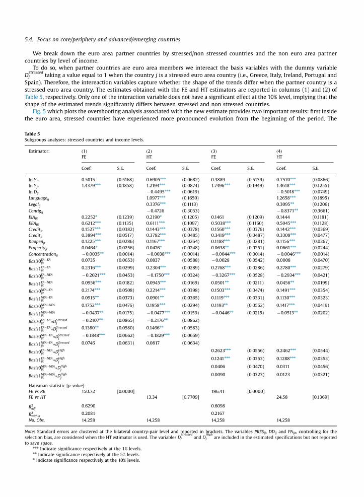
5.4. Focus on core/periphery and advanced/emerging countries

We break down the euro area partner countries by stressed/non stressed countries and the non euro area partnercountries by level of income.

To do so, when partner countries are euro area members we intereact the basis variables with the dummy variableDjStressed

taking a value equal to 1 when the country j is a stressed euro area country (i.e., Greece, Italy, Ireland, Portugal andSpain). Therefore, the intereaction variables capture whether the shape of the trends differ when the partner country is astressed euro area country. The estimates obtained with the FE and HT estimators are reported in columns (1) and (2) ofTable 5, respectively. Only one of the interaction variable does not have a significant effect at the 10% level, implying that theshape of the estimated trends significantly differs between stressed and non stressed countries.

Fig. 5 which plots the overshooting analysis associated with the new estimate provides two important results: first insidethe euro area, stressed countries have experienced more pronounced evolution from the beginning of the period. The

Table 5Subgroups analyses: stressed countries and income levels.

Estimator: ð1Þ ð2Þ ð3Þ ð4ÞFE HT FE HT

Coef. S.E. Coef. S.E. Coef. S.E. Coef. S.E.

ln Yit 0.5015 (0.5168) 0.6905nnn (0.0682) 0.3889 (0.5139) 0.7570nnn (0.0866)ln Yjt 1.4379nnn (0.1858) 1.2194nnn (0.0874) 1.7496nnn (0.1949) 1.4618nnn (0.1255)ln Dij �0.4495nnn (0.0619) �0.5018nnn (0.0749)Languageij 1.0977nnn (0.1650) 1.2658nnn (0.1895)Legalij 0.3376nnn (0.1113) 0.3095nn (0.1206)Contigij �0.4726 (0.3053) �0.8371nn (0.3661)EIAijt 0.2252n (0.1239) 0.2190n (0.1205) 0.1461 (0.1209) 0.1444 (0.1181)EEAijt 0.6212nnn (0.1135) 0.6111nnn (0.1097) 0.5038nnn (0.1160) 0.5045nnn (0.1128)Creditit 0.1527nnn (0.0382) 0.1443nnn (0.0378) 0.1560nnn (0.0376) 0.1442nnn (0.0369)Creditjt 0.3894nnn (0.0517) 0.3792nnn (0.0485) 0.3419nnn (0.0487) 0.3308nnn (0.0477)Kaopenjt 0.1225nnn (0.0286) 0.1167nnn (0.0264) 0.1188nnn (0.0281) 0.1156nnn (0.0267)Propertyjt 0.0464n (0.0256) 0.0476n (0.0248) 0.0638nn (0.0251) 0.0661nnn (0.0244)Concentrationjt �0.0035nn (0.0014) �0.0038nnn (0.0014) �0.0044nnn (0.0014) �0.0046nnn (0.0014)

Basis0EA�EAijt

0.0735 (0.0653) 0.0837 (0.0588) �0.0028 (0.0542) 0.0008 (0.0470)

Basis1EA�EAijt

0.2316nnn (0.0299) 0.2304nnn (0.0289) 0.2768nnn (0.0286) 0.2780nnn (0.0279)

Basis0EA�NEAijt

�0.2021nnn (0.0453) �0.1750nnn (0.0324) �0.3267nnn (0.0528) �0.2934nnn (0.0421)

Basis1EA�NEAijt

0.0956nnn (0.0182) 0.0945nnn (0.0169) 0.0501nn (0.0211) 0.0456nn (0.0199)

Basis0NEA�EAijt

0.2174nnn (0.0508) 0.2214nnn (0.0398) 0.1503nnn (0.0474) 0.1491nnn (0.0354)

Basis1NEA�EAijt

0.0915nn (0.0373) 0.0901nn (0.0365) 0.1119nnn (0.0331) 0.1130nnn (0.0323)

Basis0NEA�NEAijt

0.1752nnn (0.0476) 0.1958nnn (0.0294) 0.1193nn (0.0562) 0.1417nnn (0.0419)

Basis1NEA�NEAijt

�0.0437nn (0.0175) �0.0477nnn (0.0159) �0.0446nn (0.0215) �0.0513nn (0.0202)

Basis0EA�EAijt �DStressed

j�0.2107nn (0.0865) �0.2176nn (0.0862)

Basis1EA�EAijt �DStressed

j0.1380nn (0.0580) 0.1466nn (0.0583)

Basis0NEA�EAijt �DStressed

j�0.1848nnn (0.0662) �0.1829nnn (0.0659)

Basis1NEA�EAijt �DStressed

j0.0746 (0.0631) 0.0817 (0.0634)

Basis0EA�NEAijt �DHigh

j0.2623nnn (0.0556) 0.2462nnn (0.0544)

Basis1EA�NEAijt �DHigh

j0.1241nnn (0.0353) 0.1288nnn (0.0353)

Basis0NEA�NEAijt �DHigh

j0.0406 (0.0470) 0.0311 (0.0456)

Basis1NEA�NEAijt �DHigh

j0.0090 (0.0323) 0.0123 (0.0321)

Hausman statistic [p-value]:FE vs RE 150.72 [0.0000] 196.41 [0.0000]FE vs HT 13.34 [0.7709] 24.58 [0.1369]

R2adj

0.6290 0.6098

R2within

0.2081 0.2167

No. Obs. 14,258 14,258 14,258 14,258

Note: Standard errors are clustered at the bilateral country-pair level and reported in brackets. The variables PRESij, DDij and PAijt, controlling for theselection bias, are considered when the HT estimator is used. The variables Dj

Stressedand Dj

Highare included in the estimated specifications but not reported

to save space.nnn Indicate significance respectively at the 1% levels.nn Indicate significance respectively at the 5% levels.n Indicate significance respectively at the 10% levels.

1999 2001 2003 2005 2007 2009 2011

−50

−40

−30

−20

−10

0

10

20

30

40

50

years

Ove

rsho

otin

g (in

%)

vis−à−vis all euro area countriesvis−à−vis non stressed countriesvis−à−vis stressed countries

1999 2001 2003 2005 2007 2009 2011

−50

−40

−30

−20

−10

0

10

20

30

40

50

years

Ove

rsho

otin

g (in

%)

Note: The overshooting at the group level is defined in Appendix B. The grey area corresponds to the one−standard error band.The standard error for a given group in a given year is computed from the overshooting measures of the dyads belonging tothis group.

Fig. 5. Overshooting with the distinction between stressed and non stressed Euro area countries.

overshooting of stressed countries is estimated at 54% above the benchmark in 2006 versus 28% for non stressed countries.After the crisis, the decline mirrors the boomwith a level of banking activity at 56% below the benchmark level versus �24%for non stressed euro area members. In sum stressed euro area countries have experienced a stronger financial cycle thanthe rest of the area. Second, the activity of non euro area countries with their euro area partners has mostly diverged afterthe crisis. The activity towards non stressed and stressed countries was similarly at 17% above the benchmark level beforethe crisis. Then, the exposure to non stressed countries has remained steady 17% above the benchmark level; in turn, theexposure to stressed countries was 26% below the benchmark level in 2012. In sum, the withdrawal of euro area assets isheterogenous and entirely driven by the withdrawal from stressed countries assets. The international banking activitytowards stressed euro area countries has experienced a complete cycle over the period with significantly more markedevolutions inside the euro area.

Second, we interact the basis variables when partner countries are non euro area members with the dummy variableDjHigh

taking a value equal to 1 when the country j is classified as high income country in the World Bank's classification. Theinteraction variables capture whether the shape of the trends differs when the partner country is a high income country. Theestimates obtained with the FE and HT estimators are reported in columns (3) and (4) of Table 5, respectively. The inter-action variables are not significant at the 10% level for non euro area reporting countries. It means that the level of incomedoes not affect the trend outside the euro area. Conversely, the interaction variables are significant at the 1% level for euroarea reporting countries. Therefore the trend between euro area reporting countries and non euro area partner countrydepends on the level of income. In order to explicitly represent these differences, we plot the overshooting analysis on Fig. 6.We observe that the difference only matters at the beginning of the sample. In 1999, euro area reporting countries wereweakly integrated with high income non euro area countries while they were in an overshooting situation with non-advanced partner countries. After the crisis, the level of income stops mattering and the trends converge.

In total, we show that the amplitude of the cycle in the euro area has been significantly larger for stressed countries, i.e.the larger the peak, the larger the trough. In turn, for the rest of the world, the differences of income only matters before2006. Furthermore, outside the euro area, the banking integration has been a tenacious long-run trend whatever the level ofincome. The uncovered dynamics echo the waves in international capital flows described in Forbes and Warnock (2012). Weadd that the waves differ significantly across regions while Forbes and Warnock (2012) and Rey (2015) have emphasizedthat the primary factor associated with capital flow episodes is changes in global risk and not domestic conditions. Weassume that the difference may arise from a different resilience to global factors by zone, an explanation still consistent withthe global factor story.

Last but not least, explaining these patterns is unfortunately beyond the scope of our dataset. For example, to assess theeffect of rising sovereign risk on the exposure to foreign sovereign bonds as suggested in Eaton and Gersovitz (1981), oneneeds both to know the exposure to foreign sovereign bonds by dyad and to have a proxy for sovereign risk of the partnercountry such as individual sovereign credit default swap. With the aggregate sectoral exposure only (i.e. aggregatingbanking, corporate non-financial or sovereign), one cannot properly assess the marginal effect of sovereign risks on theexposure to foreign sovereign bonds because the share of sovereign claims in the aggregate sectoral exposure is unknownand varies across dyads. So the estimated marginal effect of sovereign risk upon consolidated foreign claims would not beinformative and artificially driven by the unknown breakdown. In sum, we need data of the exposure on a sectoral basis to

1999 2001 2003 2005 2007 2009 2011

−50

−40

−30

−20

−10

0

10

20

30

40

50

years

Ove

rsho

otin

g (in

%)

vis−à−vis all non euro area countriesvis−à−vis high income (non euro area) countriesvis−à−vis non high income (non euro area) countries

Note: The overshooting at the group level is defined in Appendix B. The grey areacorresponds to the one−standard error band. The standard error for a given group in agiven year is computed from the overshooting measures of the dyads belonging tothis group.

Fig. 6. Overshooting with the distinction between high income and non high income vis-à-vis countries.

explicitly test the relative relevance of these explanations. Unfortunately they are not publicly available at the dyad level.Before concluding, we present several tests to confirm the robustness of our results.

5.5. Robustness checks

The stability of our results has been evaluated with several alternative specifications of the empirical model. For the sakeof space, all estimates and corresponding graphs are available upon request in an unpublished appendix.

5.5.1. Alternative augmented specificationsWe report the estimates of the baseline specification and the estimates of an augmented specification in the main body

of the paper but much more alternative specifications could have been used.Banking crises:In a preliminary work, we considered the inclusion of dummies to control for banking crisis periods relying on the

Laeven and Valencia (2012) database. These additional variables do not alter our conclusions.Proxies for the size:We tested several variables to better control for size. First, we included stock market capitalization as a share of GDP to

better control the size; first the variable is not significant and second the lower availability of stock market capitalizationdata reduces the sample size. Second, we included Creditit to control better for the size of the source country. The resultsreported in Table 4 show that the GDP variable of the source country (ln Yit) turns non-significant when the augmentedspecification is estimated with the FE estimator.23 The smaller sample used to estimate the augmented specification and thevariable Creditit can both explain that the variable ln Yit turns non significant. To disentangle these two explanations, wehave estimated the augmented specification without the variable Creditit. The results show that the variable ln Yit remainssignificant at the 10% level. Consequently, the smaller sample used to estimate the augmented specification does not impactour results and the size effect is properly captured by the variable Creditit .

Third, we augment our specification with domestic bank assets in the reporting and destination countries in absolute terms.The variables are significant and positive as in the previous estimates including the variable credit-to-GDP (normalized by year).The corresponding overshooting graph looks similar to our core estimates with more pronounced evolutions in some cases.

Stronger asymmetries after 2006:We allowed the estimated coefficient associated with distance to vary after 2006 in order to account for stronger

asymmetries. Indeed the value of the coefficient increases in absolute terms (becomes more negative) after 2006. Theovershooting quantitative analysis changes accordingly but our conclusions remain similar.

Dummy variable for euro area membership:

23 The variable ln Yit remains significant at the 1% level when the HT estimator is used. Indeed, the Hausman test reported in Table 4 indicate that theHT estimator is consistent and more efficient than the FE estimator.

The euro area members may benefit differently from the EEA harmonization. Therefore in a robustness check, we includean additional dummy variable Euroijt taking a value equal to 1 when the dyad i and j are both euro area members. Thecoefficient associated with the variable Euroijt is not significant at the 10% level suggesting that being an euro area memberdoes not bring extra banking activity on average in comparison with being an EEA member, all things being equal.

Initial conditions:It is likely that the evolution through time depends on the original degree of cross-country integration. In order to control for

initial conditions, we include the bilateral amount of consolidated foreign claims in 1999 and start our estimate in 2000 (data arenot available for partners before 1999). The effect of this time-invariant variable can only be identified with the HT estimator. It isnot significant. However, it does not mean that initial conditions do not matter in the evolution of trends across groups. In fact,our trends are not constrained to start at the same level and it is clear on Fig. 3 that trends start at different levels across groups.

Multilateral resistance factors:Not just bilateral, but also multilateral resistance factors, the barriers that each country faces with the rest of the world,

may affect the foreign claims. The multilateral resistance terms are not directly observable. We follow Carrère (2006) tocompute the “remoteness” variable and include it in the augmented specification. The coefficient associated with thisvariable is positive and significant at the 5% level with the HT estimator and non significant at the 10% level with the FEestimator. Results are similar and our conclusions remain.

Exchange rate effects:McGuire and Wooldridge (2005, p. 81) point to the fact that exchange rate variation can affect reported positions of

consolidated foreign claims. In order to adjust for exchange rate movements, we augment our specification with the log ofbilateral real exchange rate vis-a-vis the US dollar of each reporting country and partner countries. An increase correspondsto an appreciation of the currency of country i or j, hence a depreciation of the US dollar. We expect positive signs for thesevariables. Both variables are significant and positive which confirms the overestimation of the bilateral banking activitywhen the US dollar depreciates. Results are similar and our conclusions remain.

5.5.2. Functional form of the time trendsIn order to minimize the prior on the shape of the time-trend, we use a spline function that provides flexibility to capture a non-

linear relationship. A posteriori, given the shape of the estimated trends on Fig. 3, quadratic functions may also have fitted theseevolutions. So to check the stability of our results, we run estimates using quadratic time-trends which lead to similar conclusions.

5.5.3. Choice of the benchmark in the overshooting analysisLast, the overshooting evaluation requires several methodological choices, in particular concerning the definition of the

benchmark level (see Appendix B). In the main body of the paper, the model is re-estimated without the trend variables tocompute the benchmark levels. For robustness check, we also considered as benchmark the fitted values of the dependentvariable when all the coefficients associated with trend variables (i.e., the αk in Eq. (3)) are shut down to 0. This approachdoes not require to re-estimate the model and provides similar conclusions concerning the overshooting evaluation.

6. Conclusion

We assess the evolution of international banking activity at the light of gravity equations which allow us to control forstandard determinants in order to draw international banking (dis)integration trends. Our estimates on a panel of 14 reportingcountries and their 186 partners during the period between 1999 and 2012 uncover several important stylized facts.

First, banking activity towards the euro area has been cyclical since 1999 with a peak in 2006 before the global financialcrisis (37% above the benchmark) and a severe decline after the crisis. The decline is not only a correction of the overshootingbut it is also followed by an undershooting estimated at 37% below the benchmark level, which corresponds to a markeddisintegration. We find a larger amplitude of the cycle in stressed countries than on average. In addition, euro area banks havereduced their international exposure inside and outside the euro area to a similar extent no matter the level of income. Second,the forward march of banking integration has reversed only as far as euro area countries are concerned as source or desti-nation countries. In the rest of the world, the decline of international banking activity in the aftermath of the financial crisiswas entirely due to temporary frictions. As a consequence we find no banking disintegration between non euro area countries.Third, the differences of income only matter for the banking activity from the euro area towards the rest of the world and onlybefore 2006. Outside the euro area, the banking integration has been a tenacious long-run trend whatever the level of income.

These results hopefully call for future investigations that go beyond the scope of our dataset. First, the simultaneity of theEuropean retrenchment and of the expansion of international banking activities of non-euro area members raises thequestion of a transfer of international banking activities from the euro area to non-euro area countries. Testing this transferhypothesis would require to gather and examine the data of non euro area banks market shares after 2007. Second, it wouldbe interesting to disentangle the different channels leading to the retrenchment of euro area banks. To explore suchchannels, one would need bank-level and disaggregated data distinguishing claims by sectoral exposure.

Acknowledgments

Previous versions of this paper were presented Labex-Refi seminars and CEPR-IMFS research meeting. We are grateful forcomments from seminar participants. We would like to acknowledge helpful discussions with Gunther Capelle-Blancard,Jérôme Creel, Linda Goldberg and Friederike Niepmann. We are very grateful to Amélie Guillin for sharing data on EconomicIntegration Agreements. We thank two anonymous referees for helpful comments and suggestions.

Appendix A. Spline function

A restricted cubic spline (also referred to as a natural cubic spline) is defined as a smooth polynomial function that ispiece-wise-defined. This function depends on the time trend (T) marking the number of years since the beginning of thesample in 1999 (with T ¼ 1;2;…;14). The places where the polynomial pieces connect are referred to as knots and allow oneto introduce changes in the relationship between the endogenous variable and the time trend (T).

Considering nþ2 knots at kminok1o⋯oknokmax, an unrestricted cubic spline function is written as follows (Roystonand Sauerbrei, 2007)24:

SðTÞ ¼ β00þβ10Tþβ20T2þβ30T

3þXnj ¼ 1

βj T�kj� �3

þ þβkminT�kminð Þ3þ þβkmax

T�kmaxð Þ3þ

where the plus function T�kð Þþ is defined as

T�kð Þþ ¼ T�k if TZk

0 otherwise

�

The terminology “restricted cubic spline” (or natural cubic spline) refers to the constraints imposed on SðTÞ, which implylinearity beyond the boundary knots (kmin and kmaxÞ.25 This requirement tends to avoid wild behavior near the extremesvalues of the data. Then, the restricted cubic spline function is written as (see Royston and Parmar, 2002 (p. 2194) for thealgebraic details):

SðTÞ ¼ γ0þγ1Basis0þγ2Basis1þ⋯þγnþ1Basisn

with γ0 ¼ β00, γ1 ¼ β10, γjþ1 ¼ βj for j¼ 1;…;n and

Basis0 ¼ T

Basisj ¼ T�kj� �3

þ �λj T�kminð Þ3þ �ð1�λjÞ T�kmaxð Þ3þ for j¼ 1;…;n

with λj ¼kmax�kj

kmax�kmin.

Then, the basis variables ðBasis0;…;BasisnÞ can be added to the regressors in the gravity model to capture a non-lineartime-trends that embody the evolution in the banking integration. However, the basis variables have been orthogonalizedbefore being included in the estimated specification, as suggested by Royston and Sauerbrei (2007). Without any trans-formation, the basis variables are highly correlated.

The main issue related to restricted cubic splines concerns the choice of the number of knots and their locations. Harrell(2001) recommends placing knots at equally spaced percentiles of the duration variable. In applied use, the number of knotsgenerally varies between three and seven. We use three knots (from which two basis variables are obtained) because thesample covers a limited number of years (i.e. 14 years). When three knots are considered, the default percentiles provided byHarrell (2001) are 10%, 50% and 90%. The lower and higher knots are then placed near the extreme values, and the remainingknots are placed so that the proportion of observations between the knots is constant.

Appendix B. Overshooting measure

The overshooting measure at the group level is computed in four steps.First, we compute the fitted values of the dependent variable (defined as dln CFCijt) and the fitted values of the dependent

variable when the model is re-estimated without the trend variables (defined as dln CFC�ijt).

26 The variables dln CFCijt anddln CFC�ijt correspond to predictions of the logarithm of the consolidated foreign claims.

Second, we face a re-transformation problem because we are interested in the fitted values of the level of the con-solidated foreign claims rather than their logarithm. Taking the exponential of dln CFCijt and dln CFC

�ijt is incorrect because the

24 kmin and kmax are the boundary knots and will not be placed at the extremes of T, as suggested by Harrell (2001).25 For example, the linearity constraint below kmin (i.e. when Tokmin) requires that quadratic and cubic terms must vanish, and hence, β20 ¼ β30 ¼ 0.26 The fitted values of the dependent variable when all the coefficients associated with trend variables (i.e., the αk in Eq. (3)) are shut down to 0 have

also been considered to compute dln CFC�ijt . This alternative approach to compute dln CFC

�ijt leads to similar conclusions.

error term (εijt) does not vanish in the re-transformation procedure (see Cameron and Trivedi, 2009, p. 103). We follow Duan(1983), and assuming that εijt is independent and identically distributed, we compute the fitted values of the consolidatedforeign claims as:

dCFC ijt ¼ exp dln CFC ijt

� �: expðεijtÞ;

dCFC �ijt ¼ exp dln CFC

�ijt

� �: expðεijtÞ;

where expðεijtÞ is the sample average of the exponential transformation of the error terms.Third, we define the overshooting at the dyad level as:

OSijt ¼dCFCijt� dCFC �

ijtdCFC�ijt

:

The denominator dCFC�ijt corresponds to the level of consolidated foreign claims justified by the gravity factors (i.e. the

benchmark level) and the numerator measures the gap from the benchmark due to the trend variables.Last, we compute the overshooting at the group level because trend variables are defined at the group level. Considering

only the dyads belonging to group g, we compute the overshooting measure for this group as a weighted average:

OSðgÞt ¼ ln CFCijtPij ln CFCijt

Xij

OSijt ;

where g¼EA-EA, EA-NEA, NEA-EA or NEA-NEA.

Appendix C. Supplementary data

Supplementary data associated with this paper can be found in the online version at http://dx.doi.org/10.1016/j.euroecorev.2015.10.004.

References

Adrian, T., Shin, H.S., 2009. Money, liquidity, and monetary policy. Am. Econ. Rev. 99 (2), 600–605.Al-Eyd, A.J., Berkmen, P., 2013. Fragmentation and monetary policy in the euro area. IMF Working Papers 13/208, International Monetary Fund.Baba, N., McCauley, R.N., Ramaswamy, S., 2009. US dollar money market funds and non-US banks. BIS Q. Rev. (March), 65–81.Baltagi, B.H., 2005. Econometric Analysis of Panel Data, 3rd ed. John Wiley & Sons Ltd, Chichester, UK.Baltagi, B.H., Bresson, G., Pirotte, A., 2003. Fixed effects, random effects or Hausman-Taylor? A pretest estimator. Econ. Lett. 79 (3), 361–369.Battistini, N., Pagano, M., Simonelli, S., 2014. Systemic risk and home bias in the Euro area. Econ. Policy 29, 203–251.BIS, 2003. Guide to international banking statistics. BIS Papers No. 16, Monetary and Economic Department, Bank for International Settlements.Bologna, P., Caccavaio, M., 2014. Euro area (cross-border?) banking. Questioni di Economia e Finanza (Occasional Papers) 228, Bank of Italy, Economic

Research and International Relations Area.Bouvatier, V., 2014. Heterogeneous bank regulatory standards and the cross-border supply of financial services. Econ. Model. 40, 342–354.Broner, F., Martin, A., Ventura, J., 2010. Sovereign risk and secondary markets. Am. Econ. Rev. 100 (4), 1523–1555.Brutti, F., Sauré, P.U., 2014. Repatriation of debt in the euro crisis: evidence for the secondary market theory. Working Papers 2014-03, Swiss National Bank.Buch, C.M., Neugebauer, K., Schröder, C., 2013. Changing forces of gravity: how the crisis affected international banking. Discussion Papers 48/2013,

Deutsche Bundesbank, Research Centre.Calvo, G.A., 1998. Capital flows and capital-market crises: the simple economics of sudden stops. J. Appl. Econ. 0, 35–54.Cameron, A., Trivedi, P., 2009. Microeconometrics Using Stata. Stata Press, College Station, Tex.Carrère, C., 2006. Revisiting the effects of regional trade agreements on trade flows with proper specification of the gravity model. Eur. Econ. Rev. 50 (2),

223–247.Chinn, M., Ito, H., 2006. What matters for financial development? Capital controls, institutions, and interactions. J. Dev. Econ. 81 (1), 163–192.Chinn, M., Ito, H., 2008. A new measure of financial openness. J. Comp. Policy Anal. 10 (3), 309–322.Coeurdacier, N., Martin, P., 2009. The geography of asset trade and the euro: insiders and outsiders. J. Jpn. Int. Econ. 23 (2), 90–113.De Haas, R., Van Horen, N., 2013. Running for the exit? International bank lending during a financial crisis. Rev. Financ. Stud. 26 (1), 244–285.Duan, N., 1983. Smearing estimate: a nonparametric retransformation method. J. Am. Stat. Assoc. 78 (383), 605–610.Eaton, J., Gersovitz, M., 1981. Debt with potential repudiation: theoretical and empirical analysis. Rev. Econ. Stud. 48 (April (2)), 289–309.ECB, 2014. Financial integration in Europe, European Central Bank Publications, Frankfurt am Main, Germany.European Commission, 2014. European financial stability and integration. Commission staff working document, Directorate-General Internal Market and

Services.Forbes, K.J., Warnock, F.E., 2012. Capital flow waves: surges, stops, flight, and retrenchment. J. Int. Econ. 88 (2), 235–251.Galstyan, V., Lane, P.R., 2013. Bilateral portfolio dynamics during the global financial crisis. Eur. Econ. Rev. 57 (0), 63–74.Gourinchas, P.-O., Rey, H., Truempler, K., 2012. The financial crisis and the geography of wealth transfers. J. Int. Econ. 88 (2), 266–283.Greene, W., 2003. Econometric Analysis, 5th ed. Prentice Hall, New Jersey.Guillin, A., 2013a. Assessment of tariff equivalents for services considering the zero flows. World Trade Rev. 12 (3), 549–575.Guillin, A., 2013b. Trade in services and regional trade agreements: do negotiations have to be specific?. World Econ. 36 (11), 1406–1423.Hamilton, C.B., Winters, L.A., 1992. Opening up international trade with Eastern Europe. Econ. Policy 7 (1), 77–116.Harrell, F., 2001. Regression Modeling Strategies: With Applications to Linear Models, Logistic Regression, and Survival Analysis. Springer, New York, USA.Hausman, J.A., 1978. Specification tests in econometrics. Econometrica 46 (6), 1251–1271.Hausman, J.A., Taylor, W.E., 1981. Panel data and unobservable individual effects. Econometrica 49 (6), 1377–1398.

Head, K., Mayer, T., 2014. Gravity Equations: Workhorse, Toolkit, and Cookbook. In: Gopinath, G., Helpman, E., Rogoff, K. (Eds.), chapter 3, vol. 4, Handbookof International Economics, Elsevier, pp. 131–195. http://dx.doi.org/10.1016/B978-0-444-54314-1.00003-3.

Kalemli-Ozcan, S., Papaioannou, E., Peydró, J.-L., 2010. What lies beneath the Euro's effect on financial integration? Currency risk, legal harmonization, ortrade?. J. Int. Econ. 81 (1), 75–88.

Laeven, L., Valencia, F., 2012. Systemic banking crises database: an update. IMF Working Papers 12/163, International Monetary Fund.Lane, P.R., 2006. Global bond portfolios and EMU. Int. J. Cent. Bank. 2 (2), 1–23.Lane, P.R., Milesi-Ferretti, G.M., 2012. External adjustment and the global crisis. J. Int. Econ. 88 (2), 252–265.Levine, R., 1997. Financial development and economic growth: views and agenda. J. Econ. Lit. 35 (2), 688–726.Manna, M., 2011. Home bias in interbank lending and banks' resolution regimes. Temi di discussione (Economic Working Papers) 816, Bank of Italy,

Economic Research and International Relations Area.Martin, P., Rey, H., 2004. Financial super-markets: size matters for asset trade. J. Int. Econ. 64 (2), 335–361.McGuire, P., Von Peter, G., 2009. The US dollar shortage in global banking. BIS Q. Rev. March, 47–63.McGuire, P., Wooldridge, P., 2005. The BIS consolidated banking statistics: structure, uses and recent enhancements. BIS Q. Rev. (September), 73–86.McPherson, M.Q., Trumbull, W.N., 2008. Rescuing observed fixed effects: using the Hausman-Taylor method for out-of-sample trade projections. Int. Trade

J. 22 (3), 315–340.Milesi-Ferretti, G.-M., Tamirisa, N.T., Strobbe, F., 2010. Bilateral financial linkages and global imbalances: a view on the Eve of the financial crisis. IMF

Working Papers 10/257, International Monetary Fund.Milesi-Ferretti, G.-M., Tille, C., 2011. The great retrenchment: international capital flows during the global financial crisis. Econ. Policy 26 (66), 289–346.Nilsson, L., 2000. Trade integration and the EU economic membership criteria. Eur. J. Political Econ. 16 (4), 807–827.Okawa, Y., Van Wincoop, E., 2012. Gravity in international finance. J. Int. Econ. 87 (2), 205–215.Papaioannou, E., 2009. What drives international financial flows? Politics, institutions and other determinants. J. Dev. Econ. 88 (2), 269–281.Park, S., 2002. Measuring tariff equivalents in cross-border trade in services. Working Paper No. 02-15, Korea Institute for International Economic Policy.Portes, R., Rey, H., 2005. The determinants of cross-border equity flows. J. Int. Econ. 65 (2), 269–296.Portes, R., Rey, H., Oh, Y., 2001. Information and capital flows: the determinants of transactions in financial assets. Eur. Econ. Rev. 45 (4), 783–796.Rey, H., 2015. Dilemma not trilemma: the global financial cycle and monetary policy independence. Working Paper 21162, National Bureau of Economic

Research.Royston, P., Parmar, M.K.B., 2002. Flexible parametric proportional-hazards and proportional-odds models for censored survival data, with application to

prognostic modelling and estimation of treatment effects. Stat. Med. 21 (15), 2175–2197.Royston, P., Sauerbrei, W., 2007. Multivariable modeling with cubic regression splines: a principled approach. Stata J. 7 (1), 45–70.Schildbach, J., 2011. Home, sweet home? International banking after the crisis. EU Monitor 80, Deutsche Bank Research.Schoenmaker, D., 2013. Post-crisis reversal in banking and insurance integration: an empirical survey. European Economy—Economic Papers 496, Direc-

torate General Economic and Monetary Affairs (DG ECFIN), European Commission.Shin, H.S., 2012. Global banking glut and loan risk premium. IMF Econ. Rev. 60 (2), 155–192.Verbeek, M., Nijman, T., 1992. Incomplete panels and selection bias: a survey. Discussion Paper 1992-7, Center for Economic Research, Tilburg University.Walsh, K., 2008. Trade in services: does gravity hold?. J. World Trade 42 (2), 315–334.Wang, Z.K., Winters, L.A., 1992. The trading potential of eastern europe. J. Econ. Integr. 7 (2), 113–136.Wooldridge, P., 2002. Uses of the BIS statistics: an introduction. BIS Q. Rev. March, 75–92.