Waves in space plasmas

Comprehensive Summaries of Uppsala Dissertationsfrom the Faculty of Science and Technology 869

Waves in space plasmasLower hybrid cavities and simple-pole distribution functions

BY

ANDERSTJULIN

ACTA UNIVERSITATIS UPSALIENSISUPPSALA 2003

Dissertation presented at Uppsala University to be publicly examined in 10132 (Haggsalen),Angstrom Laboratory, Uppsala, Friday, September 26, 2003 at 15:15 for the degree of Doctorof Philosophy. The examination will be conducted in English.

AbstractTjulin, A. 2003. Waves in space plasmas. Lower hybrid cavities and simple-pole distributionfunctions. Acta Universitatis Upsaliensis.Comprehensive Summaries of Uppsala Dissertationsfrom the Faculty of Science and Technology 869. 61 pp. Uppsala. ISBN 91-554-5696-0

Waves are a fundamental feature in many parts of physics, since they transport energy withouttransporting matter. This is the case also in space physics. Waves are responsible for energytransport both between different parts of space and between different particles in the spaceplasma. They are also useful for diagnostics of the space plasma itself. The present thesisconsiders two different parts of the large subject of space plasma waves: Lower hybrid cavities(LHCs) and simple-pole particle distribution functions.

The LHCs are localised density depletions that have been observed by several spacecraft.They have increased wave activity in the lower hybrid frequency range, and was previouslyfound on altitudes up to 1750 km. New observations by the Viking and Cluster satellitesshow that they are common magnetospheric features, at least up to an altitude of 35,000 km.Theoretical results, assuming a cylindrically symmetric density depletion, show that eventhough the density depletion may decrease slowly with increasing radial distance, and thusbe essentially infinite in extent, there is a maximum distance within which a trapped mode, withgiven wave numberkz parallel to the geomagnetic field, may propagate. Furthermore, there isa local relation between the plasma density gradient and the lowest possible frequency that thetrapped waves can have, for any monotonic density and givenkz. The combined theoretical andobservational results indicate that the length of the cavities is larger than the width by a factorof at least 200.

Simple-pole particle distribution functions are introduced because they can model highvelocity tails of the particle distribution in a way that is not possible to do with Maxwelliandistribution functions. These distributions also simplify the calculations. This gives newpossibilities for the physical understanding, as well as the numerical calculations, of thedispersion relations of real space plasmas. The dispersion relations of plasmas described bysimple-pole distributions are examined, both for unmagnetised and for magnetised plasmas.These examples show how particle populations with the same density and mean particle energy,but with somewhat different distribution functions, have different wave propagation propertiesthat should be observable by existing spacecraft.

Keywords: space physics, plasma, waves, dispersion relations, lower hybrid cavities, Cluster,magnetosphere

Anders Tjulin, Department of Astronomy and Space Physics, Box 515, Uppsala University,SE-75120 Uppsala, Sweden

c© Anders Tjulin 2003

ISSN 1104-232XISBN 91-554-5696-0urn:nbn:se:uu:diva-3527 (http://urn.kb.se/resolve?urn=urn:nbn:se:uu:diva-3527)

Do not wait for the futureLet the future wait for you

List of Papers

[I] Anders Tjulin. Using simple-pole distribution functions for calculations in kinetictheory of waves in a plasma.Journal of Technical Physics, 40(1):25–28, 1999.

[II] Anders Tjulin, Anders I. Eriksson, and Mats Andre. Physical interpretation ofthe Pade approximation of the plasma dispersion function.Journal of PlasmaPhysics, 64(3):287–296, 2000.

[III] Anders Tjulin and Mats Andre. The dielectric tensor of simple-pole distributionfunctions in magnetized plasmas.Physics of Plasmas, 9(5):1775–1784, 2002.

[IV] Anders Tjulin, Anders I. Eriksson, and Mats Andre. Lower hybrid cavitiesin the inner magnetosphere.Geophysical Research Letters, 30(7):1364, doi:10.1029/2003GL016 915, 2003.

[V] Anders Tjulin, Anders I. Eriksson, and Mats Andre. Localization of wave fieldsin lower hybrid cavities.Annales Geophysicae, Submitted, 2003.

[VI] Anders Tjulin, Mats Andre, Anders I. Eriksson, and Milan Maksimovic. Ob-servations of lower hybrid cavities in the inner magnetosphere by the Cluster andViking satellites.Annales Geophysicae, To be submitted, 2003.

v

List of Papers that are not included

[i] M. Andre, R. Behlke, J.-E. Wahlund, A. Vaivads, A. I. Eriksson, A. Tjulin, T. D.Carozzi, C. Cully, G. Gustafsson, D. Sundkvist, Y. Khotyaintsev, N. Cornilleau-Wehrlin, L. Rezeau, M. Maksimovic, E. Lucek, A. Balogh, M. Dunlop, P.-A.Lindqvist, F. Mozer, A. Pedersen, and A. Fazakerley. Multi-spacecraft observa-tions of broadband waves near the lower hybrid frequency at the Earthward edgeof the magnetopause.Annales Geophysicae, 19:1471–1481, 2001.

[ii] J.-E. Wahlund, A. Yilmaz, M. Backrud, D. Sundkvist, A. Vaivads, D. Winning-ham, M. Andre, A. Balogh, J. Bonnell, S. Buchert, T. Carozzi, N. Cornilleau,M. Dunlop, A. I. Eriksson, A. Fazakerley, G. Gustafsson, M. Parrot, P. Robert,and A. Tjulin. Observations of auroral broadband emissions by CLUSTER.Geo-physical Research Letters, 30(11):1563, doi:10.1029/2002GL016335, 2003.

vii

Contents

1 Introduction . . . . . . . . . . . . . . . . . . . . . . . . . . . . . . . . . . . . . . . . . . . 12 Space . . . . . . . . . . . . . . . . . . . . . . . . . . . . . . . . . . . . . . . . . . . . . . . . 3

2.1 The Earth’s magnetosphere . . . . . . . . . . . . . . . . . . . . . . . . . . . . 42.2 The Cluster satellites . . . . . . . . . . . . . . . . . . . . . . . . . . . . . . . . . 5

3 Plasma . . . . . . . . . . . . . . . . . . . . . . . . . . . . . . . . . . . . . . . . . . . . . . . 93.1 Single particle motion . . . . . . . . . . . . . . . . . . . . . . . . . . . . . . . . 103.2 Plasma as a fluid . . . . . . . . . . . . . . . . . . . . . . . . . . . . . . . . . . . . 113.3 Kinetic theory . . . . . . . . . . . . . . . . . . . . . . . . . . . . . . . . . . . . . . 12

4 Waves . . . . . . . . . . . . . . . . . . . . . . . . . . . . . . . . . . . . . . . . . . . . . . . 154.1 In theory . . . . . . . . . . . . . . . . . . . . . . . . . . . . . . . . . . . . . . . . . . 154.2 In practice . . . . . . . . . . . . . . . . . . . . . . . . . . . . . . . . . . . . . . . . . 18

5 Lower hybrid cavities . . . . . . . . . . . . . . . . . . . . . . . . . . . . . . . . . . . . 235.1 Theory . . . . . . . . . . . . . . . . . . . . . . . . . . . . . . . . . . . . . . . . . . . 235.2 Observations . . . . . . . . . . . . . . . . . . . . . . . . . . . . . . . . . . . . . . . 29

6 Simple-pole distribution functions . . . . . . . . . . . . . . . . . . . . . . . . . . 356.1 The basic idea . . . . . . . . . . . . . . . . . . . . . . . . . . . . . . . . . . . . . . 356.2 Examples . . . . . . . . . . . . . . . . . . . . . . . . . . . . . . . . . . . . . . . . . 386.3 Simple-poles in a magnetised plasma . . . . . . . . . . . . . . . . . . . . . 44

7 Future work . . . . . . . . . . . . . . . . . . . . . . . . . . . . . . . . . . . . . . . . . . . 498 Summary of the Papers . . . . . . . . . . . . . . . . . . . . . . . . . . . . . . . . . . 51

ix

1 Introduction

And I looked, and, behold, a whirlwind came out of the north, a great cloud, and afire infolding itself, and a brightness was about it, and out of the midst thereof as the

colour of amber, out of the midst of the fire.

Ezekiel 1:4, the Holy Bible (King James version)

Lights in the night sky have fascinated, inspired and frightened mankind sincethe dawn of time. They have served as omens of good or bad things to happen.The Bible, for instance, is full of references to celestial phenomena, as theexample of a possible aurora in the citation above. Phenomena like these werebelieved to have significant influence on life and death on Earth. This thesis isnot about life and death on Earth. It is, however, about waves in space plasmas.This subject is almost as large and rich as space itself, so only parts of it mayfit into this thesis.

Chapter2 describes the Earth’s magnetosphere and ionosphere, the parts ofspace closest to the Earth, and the Cluster mission, a space mission consistingof four satellites exploring this part of space. The concept of a plasma is intro-duced in chapter3 together with some different ways to characterise plasmas.Waves in plasmas are described in chapter4, both how to derive wave proper-ties theoretically and how the waves may show up in satellite data. These threechapters are thus an introduction to waves in space plasmas.

After the three introductory chapters there are two chapters where we delvedeeper into the two main topics of this thesis. Chapter5 is about lower hybridcavities, a type of wave-filled density depletions that have been found in theionosphere and the inner magnetosphere, and chapter6 is about how a plasmacan be described in terms of a simple-pole particle distribution function, andsome of the behaviour of such a plasma. Some speculations on where thisresearch may lead in the future are found in chapter7, and chapter8 containsshort summaries of the six papers that are included in this thesis.

1

2 Space

Give me more tragedy, more harmony and phantasy my dearAnd set it alight, just starting that satellite, set it alight

From the song “Sounds like a melody” by Alphaville (1984)

One of the most impressing light displays in the night sky is theAurora Bo-realis or the Northern Lights (Aurora Australis and Southern Lights on thesouthern hemisphere), which is one of the few space physics phenomena thatcan be viewed with the naked eye. Most of the discoveries in space physicshave been made by launching spacecraft to see what they encounter in space.This is for example how the lower hybrid cavities, that are discussed in chap-ter 5, were discovered. There are descriptions of auroral activity in 4000 yearold texts from China [25], but there have not been any good explanations of ituntil relatively recently. With the understanding of the aurora, the understand-ing of the relationship between phenomena on the sun and the Earth follows. Itis therefore of interest to look at some of the steps leading to this understand-ing, and thus follow the emergence of the scientific discipline of space physics[24, 25].

Some important steps leading to the understanding of the aurora were takenin Uppsala. In 1740 Anders Celsius confirmed previous observations that theneedle of a compass is always in motion. His brother-in-law Olof Hiorterdiscovered 1741 a correlation between this motion and the auroral activity. Themotion increased during auroral events. In the 19th century, AndersAngstromwas the first to perform a spectral analysis of the auroral light, and he foundthat it was the spectral lines of an excited gas.

In 1859 a great solar flare was observed simultaneously with disturbancesin the Earth’s magnetic field followed by large auroral activity 18 hours later.This established the knowledge of the connection between the sun and theEarth, with the aurora as a visible consequence. At the present we know thatthe aurora is the result when charged particles originating from the sun collidewith the Earth’s atmosphere. The motion of the charged particles is determinedby the electromagnetic fields, and the collisions excite the particles in the at-mosphere so that they emit visible light. This knowledge, however, does notdiminish the pure beauty of the polar lights on a clear night.

Since 1957, when the Soviet Union launched Sputnik I, it has been possibleto explore space in the Earth’s vicinityin situ (on location) using satellites.

3

This has greatly improved our knowledge of the physical processes in space,but it has also meant that new phenomena has been discovered, and new ques-tions need to be answered. As usual: The more you know, the more you knowthat you need to know.

2.1 The Earth’s magnetosphereThe sun does not only emit light. It also emits charged particles, the so calledsolar wind, at a rate of 109 kg per second on average. This wind has an averagevelocity of about 450 km/s at the Earth, but the Earth’s magnetic field acts asan obstacle to the solar wind so it is deflected around the Earth. The Earth’smagnetosphere is the region in space that is dominated by the Earth’s mag-netic field. Both the solar wind and the magnetosphere has charged particles,plasma, as the material content. There is a short introduction of plasma physicsin chapter3. Since the magnetic field is so important for the creation of themagnetosphere, it is more instructive to say that the magnetosphere consists ofplasmaand a magnetic field.

Spacecraft exploration of the magnetosphere has given that it has the gen-eral structure shown in figure2.1. The outer boundary of the magnetosphere iscalled themagnetopause, and it is difficult for the solar wind plasma to pene-trate this border. Upstream from the magnetopause in the solar wind we havethebow shock, where the solar wind is decelerated from supersonic to subsonicspeed. The region between the magnetopause and the bow shock is called themagnetosheath. The regions where the Earth’s magnetic field lines are con-nected to the magnetic field lines of the solar wind are called thecusp regions,and this is where the solar wind plasma most easily penetrates the magneto-sphere. Inside the magnetopause we have thelobes, where the plasma is verytenuous, about 105 particles per m3, and cold, less than 10 eV, compared withthe the solar wind (107 m−3 and 1 keV). Theplasmasheet is a region tailwardof the Earth with hot (∼ 1 keV) plasma and a density of about 106 m−3, andtheplasmasphere is a doughnut-shaped region of dense (∼ 109 m−3) and cold(∼ 1 eV) plasma. The sharp outer boundary of the plasmasphere is called theplasmapause, and it is situated at an altitude of about 4RE in the equatorialplane.

One source of the magnetospheric plasma particles is of course the solarwind. The other main source is theionosphere, which consists of particlesfrom the atmosphere that has been ionised by ultraviolet radiation from thesun. The energy source for the plasma processes in the magnetosphere is,however, almost exclusively the solar wind.

We see in figure2.1, that the magnetosphere consists of large regions withrather homogeneous plasma, separated by sharp boundaries. This structur-ing of space plasma is not unique for the Earth’s magnetosphere. The mag-

4

Plasmasphere

Plasma Sheet

Magnetosheath

Lobe

Plasmapause

Magnetopause

Lobe

Bow shock

Cusp

Earth

Figure 2.1: Schematic cross-section of the Earth’s magnetosphere. This sketchhas the sun to the left, and the Earth’s axis is vertical.

netospheres of other planets show the same basic features, with differenciesdepending on the strength of the magnetic field, the orientation of the mag-netic axis of the planet and the prescence of additional plasma sources insidethe magnetosphere, such as the moon Io in the magnetosphere of Jupiter. Wealso expect a sharp boundary between the region dominated by the solar windplasma and the interstellar medium. This outermost border of the solar systemis called theheliopause. Telescope pictures has shown features reminiscent ofmagnetospheres connected with stellar and galactic objects, so the structuringof plasmas seem to occur on many scales and in many places.

2.2 The Cluster satellitesThe Cluster mission consists of four identical satellites, flying in formationexploring the Earth’s magnetosphere [16]. It is a cornerstone mission for Eu-ropean Space Agency (ESA). An artist’s view of these spacecraft in orbit isseen in figure2.2. The formation flying has been compared to dancing, andhence the individual satellites’ names are Rumba, Salsa, Samba and Tango (fig-ure2.3). The Cluster satellites were launched in two pairs in July and August2000, and they have polar orbits around the Earth with perigee at 19,000 kmand apogee at 119,000 km. The typical distance between the satellites is be-

5

Figure 2.2: Artist’s view of the four Cluster spacecraft exploring theEarth’s magnetosphere (adapted from ESA webpages,http://sci.esa.int).

tween hundred and several thousand kilometers, depending on the phase of themission. Each satellite spins with a spin period of 4 seconds.

The point in having four identical spacecraft is that it makes it possibleto differentiate between temporal and spatial variations. As an example, weknow that the temperature in Uppsala usually is lower than the temperature inKairo, aspatial variation in temperature. We also know that the temperatureon both locations are higher at noon than at midnight, atemporal variation.This can be tested by having one thermometer in Uppsala and one in Kairo,and carefully analyse their data. We thus need more than one measuring pointfor separating spatial and temporal variations. For a three-dimensional study,as in the magnetosphere, we need at least four measuring points. Having fouridentical spacecraft makes Cluster also suitable for investigating boundaries inspace.

The examples of satellite data in chapter4, and most data used in chapter5are from the Electric Field and Wave (EFW) instrument [20] on Cluster. Thisinstrument uses four spherical probes, on each spacecraft, mounted on 44 mwire booms to measure the electric field in the satellite spin plane. The electricfield is estimated from the potential difference between two opposite probes atthe same bias current, and the distance between those probes. The instrumentnormally samples the two electric field components at 25 samples per second,but a sampling rate up to 18,000 samples per second is possible during shorttime intervals. In addition, the probe-to-spacecraft potential for each probe is

6

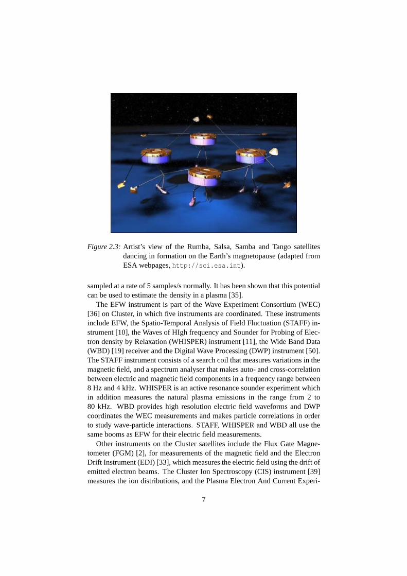
Figure 2.3: Artist’s view of the Rumba, Salsa, Samba and Tango satellitesdancing in formation on the Earth’s magnetopause (adapted fromESA webpages,http://sci.esa.int).

sampled at a rate of 5 samples/s normally. It has been shown that this potentialcan be used to estimate the density in a plasma [35].

The EFW instrument is part of the Wave Experiment Consortium (WEC)[36] on Cluster, in which five instruments are coordinated. These instrumentsinclude EFW, the Spatio-Temporal Analysis of Field Fluctuation (STAFF) in-strument [10], the Waves of HIgh frequency and Sounder for Probing of Elec-tron density by Relaxation (WHISPER) instrument [11], the Wide Band Data(WBD) [19] receiver and the Digital Wave Processing (DWP) instrument [50].The STAFF instrument consists of a search coil that measures variations in themagnetic field, and a spectrum analyser that makes auto- and cross-correlationbetween electric and magnetic field components in a frequency range between8 Hz and 4 kHz. WHISPER is an active resonance sounder experiment whichin addition measures the natural plasma emissions in the range from 2 to80 kHz. WBD provides high resolution electric field waveforms and DWPcoordinates the WEC measurements and makes particle correlations in orderto study wave-particle interactions. STAFF, WHISPER and WBD all use thesame booms as EFW for their electric field measurements.

Other instruments on the Cluster satellites include the Flux Gate Magne-tometer (FGM) [2], for measurements of the magnetic field and the ElectronDrift Instrument (EDI) [33], which measures the electric field using the drift ofemitted electron beams. The Cluster Ion Spectroscopy (CIS) instrument [39]measures the ion distributions, and the Plasma Electron And Current Experi-

7

ment (PEACE) [23] measures the electron distribution function. The Researchwith Adaptive Particle Image Detectors (RAPID) instrument [49] measures theenergetic particles and the Active Spacecraft POtential Control (ASPOC) ex-periment [40] keeps the spacecraft potential low with respect to the plasma, inorder to enable accurate particle measurements of the cold plasma population.

8

3 Plasma

“Sometimes reality is too complex for oral communication. But legend embodies it ina form which enables it to spread all over the world.”

From the film “Alphaville” directed by Jean-Luc Godard (1965)

A plasma may be defined as an ionised gas in which collective effects are im-portant [8, 17]. The condition that the particles are ionised means that theyare electrically charged, and hence the particle motion in a plasma depends onthe electric and magnetic fields that the particles experience. These fields arefurthermore in part caused by the motion of the charged particles themselves.The condition that the plasma should exhibit collective behaviour means thatthese long-range electromagnetic forces should be more important than inter-actions between neighbouring particles for the particle motion in the plasma.This condition is satisfied when there are many charged particles within theDebye sphere of each ion, where the Debye sphere is the volume inside whichan individual ion’s electric field influences its surroundings. The result is thatall particles in a plasma interact at distance, to compare with a neutral gaswhere the particle motion is only dependent on collisions between neighbour-ing particles. This fact leads to several interesting and complex phenomenain a plasma [28], and this behaviour, fundamentally different from that of aneutral gas, means that is is reasonable to consider plasma as the fourth stateof matter, besides solid, fluid and gas.

More than 99% of the observed matter in the universe is in the plasma state,but plasmas are rather rare on the surface of the Earth with lightning dischargesas one of the few natural occuring examples. When we travel up through ouratmosphere, the gas gets more ionised at higher altitudes because of photo-ionisation processes, and at about 80 km we may start considering it a plasma.Most of the phenomena that we encounter with a satellite is thus occuringin a plasma environment, so in order to understand what we see, we mustunderstand the properties of a plasma. On the other hand, we may also usespace as a large plasma laboratory in which we can study processes that arenot possible to study in a laboratory on the surface of the Earth. Space andplasma physics are consequently closely related to each other.

9

3.1 Single particle motionWe start by examining the simple situation with the motion of a charged parti-cle in fields that are constant in space and time. The total force on this particleis given by

�F = q(�E +�v×�B

)+�Fg, (3.1)

whereq is the charge of the particle,�v its velocity,�E and�B the electric andmagnetic fields and�Fg the total non-electromagnetic force acting on the parti-cle. The equation of motion for this particle is then

md�vdt

= q(�E +�v×�B

)+�Fg, (3.2)

wherem is the mass of the particle. To be able to analyse the particle motion,we introduce a velocity�u defined by

�u =�v−(�E +�Fg/q

)×�B

B2 =�v−�vd, (3.3)

which can be interpreted as the particle velocity seen in a reference frame withvelocity�vd. After some vector algebra, and using the fact that the backgroundfields in this example do not vary in time, the equation of motion in this newframe becomes

md�udt

= q(�E‖ +�u×�B

)+�Fg‖, (3.4)

where the subscript‖ denotes the field component parallel to the magneticfield. If we in addition introduce the subscript⊥ for the components perpen-dicular to the magnetic field, the equation of motion can be separated into aparallel part

mdv‖dt

= qE‖ +Fg‖, (3.5)

where we have transformed back to the original reference frame, knowing thatu‖ = v‖, and a perpendicular part

md�u⊥dt

= q�u⊥×B. (3.6)

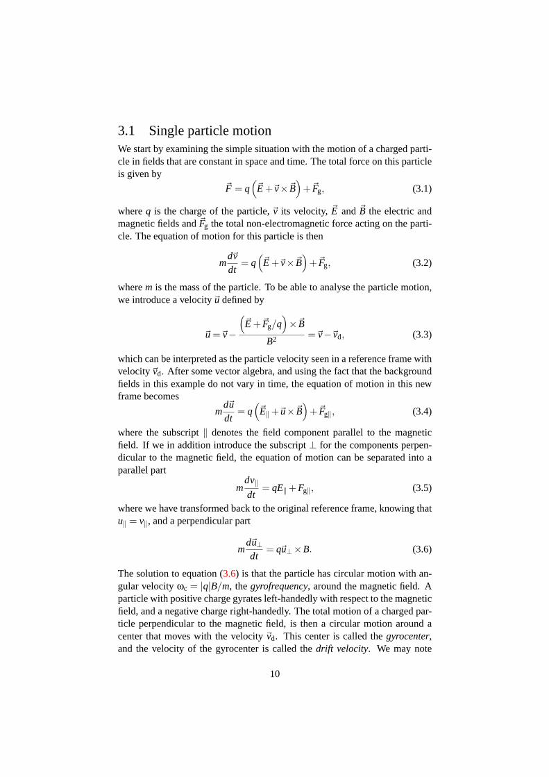
The solution to equation (3.6) is that the particle has circular motion with an-gular velocityωc = |q|B/m, thegyrofrequency, around the magnetic field. Aparticle with positive charge gyrates left-handedly with respect to the magneticfield, and a negative charge right-handedly. The total motion of a charged par-ticle perpendicular to the magnetic field, is then a circular motion around acenter that moves with the velocity�vd. This center is called thegyrocenter,and the velocity of the gyrocenter is called thedrift velocity. We may note

10

vd

E

B

Figure 3.1: The drift motion for a positive charge in constant electric and mag-netic fields. The magnetic field is pointing into the paper.

that if �Fg = 0, the direction of the drift velocity is independent of the charge ofthe particle, in contrast to the direction of the circular motion around the mag-netic field. An example of this drift motion for a positively charged particle inconstant electric and magnetic fields is shown in figure3.1.

It is clear that even in this very simple example, the particle motion be-comes somewhat complex. The situation becomes more complicated when weconsider fields that are not constant in space or time [17]. This is the casefor a plasma, where each particle is moving in the electric and magnetic fieldsfrom all other particles in the plasma. It is, in principle, possible to use theequation of motion for all particles in a plasma for determining the behaviourof the plasma, but the number of equations will then be completely intractable.There are however ways of simplifying the description of a plasma.

3.2 Plasma as a fluidWe may derive fluid equations for each particle species in the plasma. The firstof these equations is thecontinuity equation

∂nα

∂t+∇ · (nα�uα) = 0, (3.7)

wherenα is the number density and�uα is the fluid velocity of particle speciesα. This equation says that the change of the number of particles inside a givenvolume is equal to the number of particles passing through the surface of thatvolume. There is also amomentum equation for each particle species. It isgiven by

mα

(∂�uα

∂t+(�uα ·∇)�uα

)= qα

(�E +�uα ×�B

)−∇ · ¯Pα, (3.8)

11

where ¯Pα is the pressure tensor. If the pressure is isotropic, or near isotropic,we may replace∇ · ¯Pα with the gradient of a scalar pressure∇pα. Equa-tion (3.8) describes the fluid motion of particle speciesα under the influenceof electromagnetic forces and pressure. In addition, we need anequation ofstate describing how the pressure varies in time. In thecold plasma approxi-mation the pressure term in equation (3.8) is neglected in order to simplify thecalculations. This is the approximation that is used in chapter5.

In addition to the equations that each particle species must obey, we mustalso include Maxwell’s equations that are determining the electromagneticfields. They are

∇ ·�E =ρε0

(3.9)

∇×�E = −∂�B∂t

(3.10)

∇ ·�B = 0 (3.11)

∇×�B = µ0�J +1c2

∂�E∂t

, (3.12)

whereρ is the total charge density and�J the total current density. These twoquantities are given by

ρ = ∑α

qαnα (3.13)

�J = ∑α

qαnα�uα, (3.14)

where the summations are made over all particle species in the plasma.The set of equations we have found in this section is useful for many of

the phenomena we encounter in space plasmas, but it may be too simplified insome situations. Sometimes the dynamics of the individual particles has to betaken into account in addition, and that is where theplasma kinetic theory isused. The next section gives a short introduction to this subject.

3.3 Kinetic theoryIn plasma kinetic theory the plasma is described in terms of itsparticle dis-tribution functions. The distribution function,fα(�x,�v, t), describes the particledensity in the six-dimensional phase space for particle speciesα. The numberdensity is calculated fromfα(�x,�v, t) by integrating over all velocities

nα(�x, t) =Z

fα(�x,�v, t)d3v. (3.15)

12

Other macroscopic quantities such as the fluid velocity and the pressure canalso be determined using different integrals of the distribution function. Whenthe plasma is in thermal equilibrium, the distribution function is given by aMaxwellian

fM(�v) =n0

vth√

πe−v2/v2

th, (3.16)

wherev = |�v|, andvth is the thermal velocity. The normalisation factors in frontof the exponential are there to satisfy equation (3.15). In chapter6 we will useanother type of distribution function, the simple-pole distribution, to describea plasma.

The equation that determines the time evolution of the distribution functionfα(�x,�v, t) is theBoltzmann equation

∂ fα

∂t+�v ·∇ fα +

�Fα

mα·∇�v fα =

(∂ fα

∂t

)coll.

, (3.17)

where the right hand side describes the rate of change offα due to particlecollisions. �Fα is the total force acting on particle speciesα, and the operator∇�v means the gradient with respect to the velocity. We will henceforth onlyconsider collisioness plasma where the Lorentz force is the only force actingon the particles, so the Boltzmann equation we use here is of the form

∂ fα

∂t+�v ·∇ fα +

qα

mα

(�E +�v×�B

)·∇�v fα = 0. (3.18)

This equation is usually called theVlasov equation. The electric and mag-netic fields are given by Maxwell’s equations (3.9–3.12), with the total chargedensity in this case given by

ρ(�x, t) = ∑α

qα

Zfα(�x,�v, t)d3v, (3.19)

and the total current density by

�J(�x, t) = ∑α

qα

Zfα(�x,�v, t)�vd3v. (3.20)

The summations here are made over all particle species in the plasma.

13

4 Waves

I have before me all the necessary elements:it is their combination that eludes me.

From the song “I trawl the Megahertz” by Paddy McAloon (2003)

Waves are important in many parts of physics since they enable transport ofenergy without transport of matter. For a familiar example of waves, let usconsider sound waves. When we speak, our lungs act as an energy sourcethat push air through our vocal cords where sound waves are generated. Thesewaves are then propagating through the air to the ears of the listeners, where thewaves cause their eardrums to vibrate. The energy, not the air, from our lungsis thus transfered to their eardrums via the generation of sound waves. Theenergy in this example originates from the sun, although rather indirectly. Thesunlight has, through photosynthesis, been converted into chemically boundenergy in the apple tree whose fruit gave us the energy we needed to be able totalk.

Waves also play an important role in space physics, where plasma is themedium in which they propagate. Energy transport between regions in spaceis often made through waves and the sun is, somewhat more obvious thanin the example above, usually the energy source for the wave phenomena inthe Earth’s magnetosphere. Waves are also important for transport of energybetween the different particles in a plasma, and it is also possible to makediagnostics of a plasma by examining its wave emissions. The plasma num-ber density can for example be found by examining the wave spectrum. TheEarth’s magnetosphere is filled with a multitude of waves with different fre-quencies and behaviour. In the following, we use different plasma models toinvestigate what waves we can find in different types of plasmas.

4.1 In theoryWe investigate wave properties of a plasma by examining the response to smallperturbations in the plasma parameters. The standard procedure is to assumethat a plasma parameterχ(�r, t) can be written as

χ(�r, t) = χ0 +χ1(�r, t), (4.1)

15

whereχ1(�r, t) is a small perturbation to the background valueχ0. Usually ina homogeneous plasma the perturbations are assumed to be plane waves ofharmonic form

χ1(�r, t) = χ1ei(�k·�r−ωt). (4.2)

This makes it possible to substitute the time derivative∂/∂t with −iω and thegradient∇ with i�k in the equations. In chapter5 we analyse a situation wherethe plasma is inhomogeneous with a cylindrical geometry, which makes us usea slightly different way to describe the perturbations. Using the above assump-tions in the plasma equations from chapter3 and onlylinear perturbations, thatis we neglect all terms where the perturbed quantities are of second order orhigher, we derivedispersion relations. These are relations between the waveangular frequency,ω, and the wave vector,�k, that are possible in the plasma.

As an example we consider electron oscillations in a cold plasma with nobackground electromagnetic fields at a sufficiently short time scale so thatthe ions can be considered stationary. Using the equations from the fluid de-scription of a plasma in chapter3.2, we see that the electron continuity equa-tion (3.7) gives the following expression for the electron density perturbations

ne =n0

ω�k ·�ue, (4.3)

wheren0 is the background density (and the ion density). The momentumequation (3.8) for the electrons gives an electron fluid velocity of

�ue = −ie

meω�E, (4.4)

which means that Gauss’ law (3.9) turns into

�k ·�E = ieε0

ne = ien0

ωε0

�k ·�ue =e2n0

ω2ε0me

�k ·�E, (4.5)

where we have used equations (4.3) and (4.4). This equation can only be sat-isfied if the angular frequency of the oscillations satisfies

ω2 =e2n0

ε0me= ω2

pe. (4.6)

The frequencyωpe of these oscillations is called theelectron plasma frequencyand it is one of the fundamental frequencies in a plasma.

It is of course interesting to look at all possible waves in a cold plasma.Using the fluid description, assuming that there is no background fluid mo-tion of the plasma and no background electric field, we get the cold plasmadispersion relation which can be found in many textbooks in plasma physics[3, 17, 45, 46]. A convenient way of displaying dispersion relations is to usedispersion surfaces [1] which showω as a function of�k. In figure4.1we have

16

10−1

100

10−1

100

0

0.5

1

1.5

2

2.5

3

k⊥ c / ω

ce

k|| c / ω

ce

ω /

ωce

Figure 4.1: The dispersion surfaces in a cold plasma. In this example we havean electron-proton plasma withωpe = 0.55ωce.

an example where we see the dispersion surfaces in a cold electron-protonplasma, where the electron plasma frequency,ωpe, is 0.55 times the electrongyro frequency,ωce. We see that there are several different wave modes al-ready in this simple cold plasma example.

We may also find dispersion relations in a plasma described by plasma ki-netic theory, as in chapter3.3, but for general magnetised plasmas these re-lations are complicated expressions [5, 46]. It is, however, possible to find asimple expression in the case of an unmagnetised homogeneous plasma. Thedispersion relation in that situation is given by [41]

1−∑α

ω2pα

nα0

Z ∞

−∞

fα0(v)

(ω− kv)2 dv = 0. (4.7)

Here fα0(v) denotes the unperturbed distribution function for plasma particlespeciesα and the summation is over all particle species in the plasma. Thepath of integration is understood to be along the real axis, except that it goesbelow the phase velocity pole inv = ω/k, even in the case where Im(ω/k) < 0.Equation4.7will be used in chapter6 as well as the magnetised version of thekinetic dispersion relation [5].

We have several different waves even in the simple case of a cold plasmawith only two particle species, as we saw in the dispersion surfaces in fig-ure 4.1. The waves in a plasma have been divided into different subsets dueto their features, in order to keep track of them. Depending on the directionof the wave vector,�k, with respect to the background magnetic field,�B0, wedistinguish betweenparallel andperpendicular waves. The polarisation of thewave electric field separates betweentransversal waves with�E ⊥�k and lon-gitudinal waves with �E ‖�k. Electrostatic waves have no wave magnetic field

17

component, which theelectromagnetic waves have.Right-handed waves havea wave electric field vector going in a right-handed direction with respect to thebackground magnetic field; the direction in which the electrons are gyrating.The left-handed waves have left-handed wave electric field. In chapter5, wewill encounter waves where the wave vector,�k, is rotating right-handedly orleft-handedly with respect to the magnetic field.

The analysis of the waves in lower hybrid cavities that is done in chapter5 isconsidering electrostatic waves in a slightly inhomogeneous plasma describedby the cold plasma fluid equations. In chapter6, both electrostatic and electro-magnetic waves are examined in a homogeneous plasma that is described bysimple-pole distribution functions.

4.2 In practiceThe previous section included a theoretical approach to the waves in a plasma.In this section we investigate what can be said about the waves in space bylooking at satellite data. The example that will be examined here use datafrom the EFW instrument [20] on Cluster [16]. We have a dataset, that isabout eleven seconds long, of probe-to-spacecraft potential that is sampled at9000 samples/s using a low-pass filter at 4 kHz. The data is from December 19,2002, and is taken very close to the plasmapause (see figure2.1) in the innermagnetosphere on the dawn side of the Earth. Only data from three probes areused in this example because of a failure on one of the probes on the satellitein question (Cluster 3, Samba) that occured on July 29, 2002.

The first thing we must do is to transform the potential data to electric fielddata. The potential difference between two probes divided by the distance isthe normal way of estimating the electric field. Because of the probe failure,one of the electric field components has to be estimated using the potential dif-ference between the probe and the satellite body, subtracting the mean value.The two electric field components we have now are in a coordinate systemspinning together with the satellite. After transforming into a coordinate sys-tem fixed with respect to the Earth, we get the two electric field componentsthat are shown in figure4.2. These waveforms will be explored further. Themagnetic field in this example is within 20◦ from the satellite spin axis, andhence the measured electric field components are nearly perpendicular to thebackground magnetic field.

Just looking at the two waveforms does not give much information. Wemay, however, transform the data into sound waves and listen to it. This exam-ple sounds like birds singing in the morning, the dawn chorus, and thus we canidentify the data as an example of achorus emission. This is a known wavephenomenon in the regions of the magnetosphere where the data were taken[29].

18

−20

0

20

Ex [

mV

/m]

11:20:10 11:20:15 11:20:20−20

0

20

UT

Ey [

mV

/m]

Figure 4.2: Waveforms of the sunward (upper panel) and the duskward (lowerpanel) electric field. The data come from Cluster 3 (Samba) 2002-12-19, and were taken very close to the plasmapause in the innermagnetosphere of the Earth.

0 500 1000 1500 2000 2500 3000 3500 4000 4500

10−5

10−3

Frequency [Hz]

PS

D [

(mV

/m)2 /H

z]

Figure 4.3: The power spectral density for the sunward (dashed line) and theduskward (solid line) electric field data from figure4.2.

In order to investigate the spectral contents of the data we can useFourieranalysis, which says that almost every function can be expressed as a sum ofits harmonic components. The coefficients for these components can be usedto calculate thepower spectral density (PSD) [14] of the signal. This quantitytells how much wave power we have for each frequency. The task to find theFourier components from measured data is simplified by using theFast FourierTransform (FFT) algorithm [6, 9]. The power spectral density of our exampleis shown in figure4.3. We see that most of the wave power is at frequenciesabove 2 kHz, and we may also note that the low-pass filter at 4 kHz seemsto work well. This spectrum can be considered an average spectrum over thewhole data interval, but we see from the waveform (and we heard) that there isa clear time dependence of the signal which cannot be seen in the spectrum.

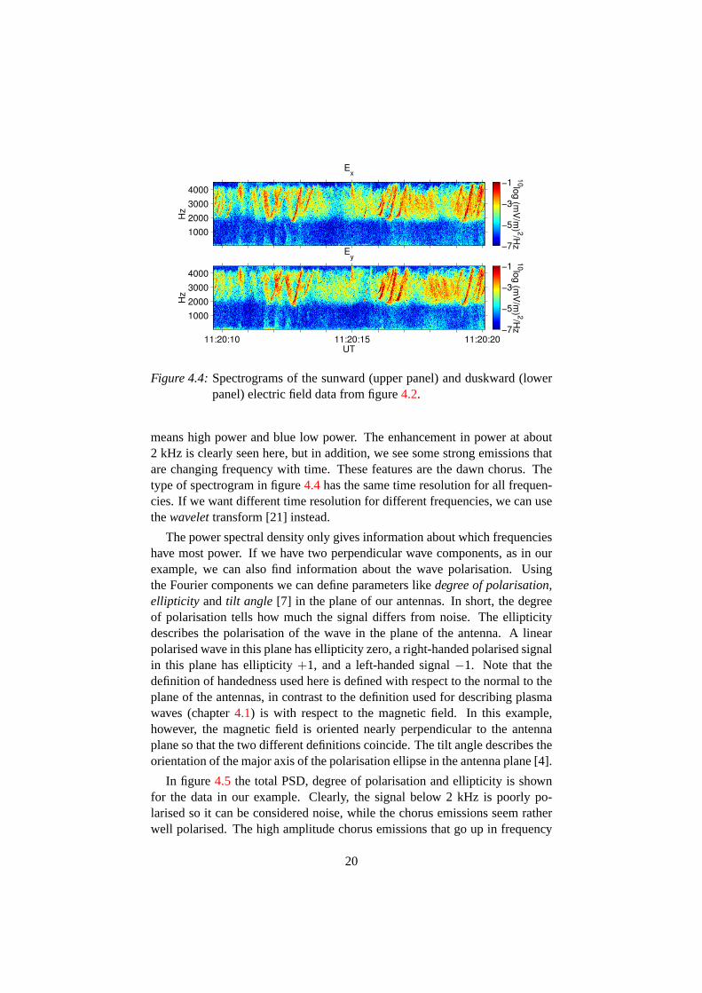
A standard way of investigating a dynamic signal, like the one in our exam-ple, is to divide the time series in smaller time intervals and find the PSD foreach of these intervals. This is usually displayed as aspectrogram, as in fig-ure4.4. In a spectrogram we have time and frequency on the axes and the PSDfor each time-step and frequency is displayed by the color. In figure4.4, red

19

−7

−5

−3

−1H

z

Ex 10log (m

V/m

) 2/Hz

1000

2000

3000

4000

−7

−5

−3

−1

UT

Hz

Ey 10log (m

V/m

) 2/Hz

11:20:10 11:20:15 11:20:20

1000

2000

3000

4000

Figure 4.4: Spectrograms of the sunward (upper panel) and duskward (lowerpanel) electric field data from figure4.2.

means high power and blue low power. The enhancement in power at about2 kHz is clearly seen here, but in addition, we see some strong emissions thatare changing frequency with time. These features are the dawn chorus. Thetype of spectrogram in figure4.4has the same time resolution for all frequen-cies. If we want different time resolution for different frequencies, we can usethewavelet transform [21] instead.

The power spectral density only gives information about which frequencieshave most power. If we have two perpendicular wave components, as in ourexample, we can also find information about the wave polarisation. Usingthe Fourier components we can define parameters likedegree of polarisation,ellipticity andtilt angle [7] in the plane of our antennas. In short, the degreeof polarisation tells how much the signal differs from noise. The ellipticitydescribes the polarisation of the wave in the plane of the antenna. A linearpolarised wave in this plane has ellipticity zero, a right-handed polarised signalin this plane has ellipticity+1, and a left-handed signal−1. Note that thedefinition of handedness used here is defined with respect to the normal to theplane of the antennas, in contrast to the definition used for describing plasmawaves (chapter4.1) is with respect to the magnetic field. In this example,however, the magnetic field is oriented nearly perpendicular to the antennaplane so that the two different definitions coincide. The tilt angle describes theorientation of the major axis of the polarisation ellipse in the antenna plane [4].

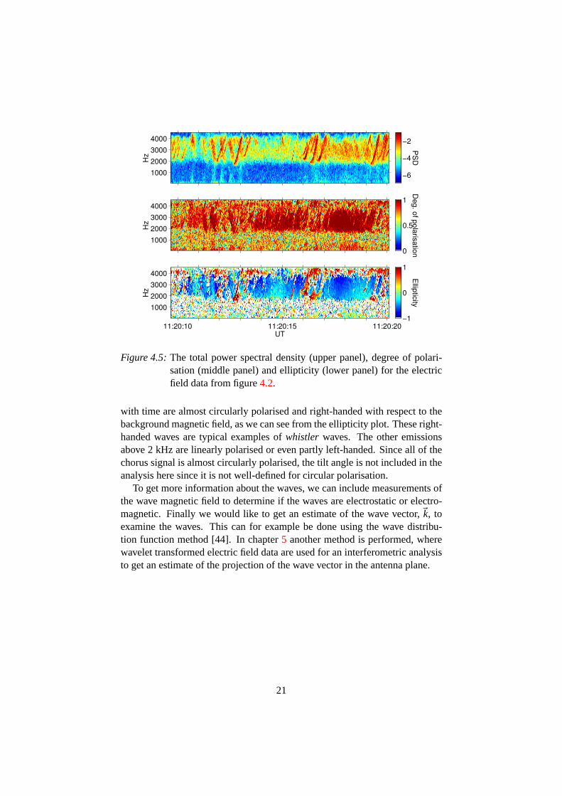
In figure 4.5 the total PSD, degree of polarisation and ellipticity is shownfor the data in our example. Clearly, the signal below 2 kHz is poorly po-larised so it can be considered noise, while the chorus emissions seem ratherwell polarised. The high amplitude chorus emissions that go up in frequency

20

−6

−4

−2H

zP

SD

1000

2000

3000

4000

0

0.5

1

Hz

Deg. of polarisation

1000

2000

3000

4000

−1

0

1

UT

Hz

Ellipticity

11:20:10 11:20:15 11:20:20

1000

2000

3000

4000

Figure 4.5: The total power spectral density (upper panel), degree of polari-sation (middle panel) and ellipticity (lower panel) for the electricfield data from figure4.2.

with time are almost circularly polarised and right-handed with respect to thebackground magnetic field, as we can see from the ellipticity plot. These right-handed waves are typical examples ofwhistler waves. The other emissionsabove 2 kHz are linearly polarised or even partly left-handed. Since all of thechorus signal is almost circularly polarised, the tilt angle is not included in theanalysis here since it is not well-defined for circular polarisation.

To get more information about the waves, we can include measurements ofthe wave magnetic field to determine if the waves are electrostatic or electro-magnetic. Finally we would like to get an estimate of the wave vector,�k, toexamine the waves. This can for example be done using the wave distribu-tion function method [44]. In chapter5 another method is performed, wherewavelet transformed electric field data are used for an interferometric analysisto get an estimate of the projection of the wave vector in the antenna plane.

21

5 Lower hybrid cavities

Right and left; the hothouse and the street. The Right can only live and workhermetically, in the hothouse of the past, while outside the Left prosecute their affairsin the streets manipulated by mob violence. And cannot live but in the dreamscape of

the future.

From the novel “V” by Thomas Pynchon (1963)

A lower hybrid cavity (LHC) (or lower hybrid solitary structure, LHSS) is alocalised density depletion with increased wave amplitude in the lower hybridfrequency range. LHCs have been observed in the ionosphere by soundingrockets [27, 31, 38, 47] and the Freja satellite [12, 15, 22, 34], and they haverecently been identified further out in the magnetosphere in Viking and Clus-ter data (see Paper IV). The observed LHCs have cylindrical geometry withsymmetry axis along the background magnetic field. The radius of a typicalobserved cavity is a couple of ion gyro radii, and the observed depth of thedensity depletion varies from 0.1% to 90%. The parallel size of the cavity ismuch larger than the perpendicular size, so LHCs are very elongated densitydepletions [42]. Statistical investigations have shown that the observed LHCsare stationary structures, at least on the time scale of the spacecraft passingthe LHC which for the Freja observations is about 10 ms [26] and for Clusterabout 100 ms. The fact that LHCs are rather stable makes it interesting to ex-amine what waves we may find in a density depletion, since there is sufficienttime for the wave emissions to reach a stationary state. In the following wederive the equations of the plasma model that is used in Paper V to investigatethe wave properties of an LHC. This is followed by an example of an LHCobservation from the Cluster dataset.

5.1 TheoryThe observed waves in a lower hybrid cavity are in the lower hybrid frequencyrange, so we will assume that we are in that range of frequencies here. For theplasma in the magnetospheric regions that we consider here, whereωci � ωpi,this condition on the frequencies means that the wave angular frequency,ω,satisfiesωci � ω � ωce. Hereωci is the ion cyclotron frequency,ωpi the ionplasma frequency andωce the electron cyclotron frequency. For simplicity,

23

we will consider a cold plasma with only one ion species in the theory. Thebasic set of equations we use here are the cold plasma fluid equations fromchapter3.2, that was also used in chapter4.1.

The continuity equation (3.7) for the ions can be written

∂Ni

∂t+∇ · (Ni�ui) = 0, (5.1)

whereNi is the ion number density and�ui the velocity of the ion fluid. Theconditionωci � ω means that we can consider the ions to be unmagnetised,and thus the magnetic term in the momentum equation (3.8) for the ions can beneglected. The momentum equation, assuming the ions to be singly ionised, isthen given by

mi

(∂�ui

∂t+(�ui ·∇)�ui

)= e�E, (5.2)

wheremi is the ion mass,�E is the electric field ande is the elementary charge.For the electrons, the conditionω � ωce gives us that the time scale is so

long that the electrons make several gyrations during one wave period. Theelectron motion perpendicular to the background magnetic field is thus givenby their gyrocenter drift motion, as in the example in chapter3.1and figure3.1.For the electron motion along the magnetic field, we have to include accelera-tion due to the electric field. We then have

�ue⊥ =�udrift⊥ (5.3)

for the electron motion perpendicular to the magnetic field,�ue⊥, and

me

(∂ue‖∂t

+(�ue ·∇)ue‖

)= −eE‖ (5.4)

for the electron motion along the magnetic field whereme is the electron mass.The subscript⊥ denotes the vector component perpendicular to the magneticfield and the subscript‖ denotes the vector component along the magneticfield. The continuity equation for the electrons is given by

∂Ne

∂t+∇ · (Ne�ue) = 0, (5.5)

whereNe is the electron number density.The perpendicular electron drift�udrift⊥ consists of many different terms.

The most important contribution to this drift is the electron drift across themagnetic field that we found in chapter3.1,

�uE =�E ×�B

B2 , (5.6)

24

where�B is the magnetic field. We also need to include the polarisation drift[17]

�upol = − me

eB2

d�E⊥dt

= − me

eB2

(∂�E⊥∂t

+(�ue ·∇)�E⊥

), (5.7)

that is a consequence of the electric field being time dependent. In order touse this expression we have assumed that the time scale for the electric fieldvariations is longer than one gyroperiod of the electrons, but this follows fromthe assumptionω � ωce that we have already used. Other drifts, such as thosecoming from small non-uniformities in the magnetic field and the magneticfield varying in time, will be neglected here. This means that we from now ononly consider electrostatic perturbations in the plasma.

In order to linearise the equations we may assume that the particle numberdensities are given byNi = n + ni andNe = n + ne wheren is the backgrounddensity, constant in time but with a spatial dependence, andni andne are smallperturbations to this density. The magnetic field is given by its backgroundvalue�B0. We also note that|�upol| � |�uE|, and assume that there is no fluidvelocities in the unperturbed plasma. Furthermore, we use a velocity potentialψ to describe the ion motion,�ui = ∇ψ. This can be done since we are consid-ering unmagnetised ions, and the ion motion in that case only depends on theelectrostatic forces. The ion motion is thus irrotational on these time scales.

The linearised equations for the ions are

∂ni

∂t+n∇2ψ = 0 (5.8)

and

mi∂ψ∂t

= −eφ, (5.9)

whereφ is the normal electrostatic potential,�E = −∇φ. The continuity equa-tion for the electrons turns into

∂ne

∂t+n(∇ · (�uE +�upol +�ue‖

))+�uE ·∇n = 0. (5.10)

This equation can be simplified if we note that∇ ·�uE = 0 in the electrostaticapproximation that we use here. We also note that the divergence of the polar-isation drift in linearised form is given by

∇ ·�upol = − ∂∂t

(me

eB20

∇ ·�E⊥)

. (5.11)

We may now introduce a modified density,ζ, defined by

ζ = ne− nme

eB20

∇ ·�E⊥, (5.12)

25

in order to simplify the expressions. The electron continuity equation can nowbe written as

∂ζ∂t

+n(∇ ·�ue‖

)+�uE ·∇n = 0, (5.13)

where we also have used|�upol| � |�uE|, and assumed that the density gradientis perpendicular to the magnetic field. The linearised momentum equation forthe electron motion along the magnetic field is given by

me∂ue‖∂t

= −eE‖. (5.14)

Finally, to close the system of equations, we use Gauss’ law for the electricfield

∇ ·�E =eε0

(ni −ne) , (5.15)

whereε0 is the permittivity of empty space.Our equations can be simplified further if we assume that the background

magnetic field is in the ˆz direction and we fully introduce the electrostaticpotentialφ in our equations. Furthermore, we assume that the gradients ofthe parameters are larger across than along the magnetic field. Finally, weintroduce the variation in background density,ν(�r), so that the backgrounddensity is given byn(�r) = n0(1+ν(�r)), wheren0 is a constant density. Thesystem of equations is then

∂ni

∂t= −n0∇2

⊥ψ (5.16)

∂ψ∂t

= − emi

φ (5.17)

∂ζ∂t

−n0∇⊥φ× z

B0·∇⊥ν = −n0

∂ue‖∂z

(5.18)

∂ue‖∂t

=e

me

∂φ∂z

(5.19)

∇2⊥φ = − e

ε0(ni −ne) (5.20)

ζ = ne+n0me

eB20

∇2⊥φ, (5.21)

where we have assumed that the density variation is small compared with thebackground density (ν � 1). This is the set of equations that we will use forexamining the waves in the lower hybrid cavities.

In summary: We are looking at a situation where, during one wave period,the ions are considered unmagnetised and the electron motion is given by theelectron drift velocity. This approximation is sometimes called the Hall ap-proximation. In addition, we are using cold plasma electrostatic theory, and

26

we assume that all perpendicular gradients are larger than the parallel gradi-ents.

As a test of this set of equations we look at plane waves in a homogeneousplasma. We have in that caseν = 0, and may use Fourier transforms. Thetransformed version of the system of equations is given by

− iωni = n0k2⊥ψ (5.22)

−iωψ = − emi

φ (5.23)

−iωζ = −in0kzue‖ (5.24)

−iωue‖ = ie

mekzφ (5.25)

−k2⊥φ = − e

ε0(ni −ne) (5.26)

ζ = ne− n0me

eB20

k2⊥φ. (5.27)

By combining the above equations we find that the ion density perturbationsare given by

ni =n0k2

⊥e

miω2 φ, (5.28)

and the electron density perturbations by

ne =(−n0ek2

z

meω2 +n0mek2

⊥eB2

0

)φ. (5.29)

If these density perturbations are inserted in Gauss’ law, we get a dispersionrelation of the form

ω2 = ω2LH

(1+

mi

me

k2z

k2⊥

), (5.30)

where thelower hybrid frequency, ωLH, is given by

ω2LH =

ω2ceω2

pi

ω2pe+ω2

ce. (5.31)

This result is what we expect for this situation: The dispersion relation forlower hybrid waves in a homogeneous plasma [46].

The lower hybrid cavities are known to be cylindrical symmetric densitystructures aligned with the background magnetic field. This means that thebackground density variation is given byν(�r) = ν(ρ), whereρ is the radialdistance from the symmetry axis. We may also assume the perturbed quantitiesto be of the form

f (ρ,ϕ,z, t) = f (ρ)ei(mϕ+kz−ωt), (5.32)

27

wherem is an integer. The relative sign betweenω andm determines if theperturbations are right-handed (same sign) or left-handed (different sign). Herewe assume thatm to be positive, which means that the sign ofω determinesthe handedness of the waves. Note that this is not the same as the handednessof the wave polarisation that was introduced in chapter4.

If we use these assumptions in the previous equations, we get an interestingresult for a general shape of the density depletionν(ρ) (see Paper V). There isa radius inside which we have waves with frequencies below the lower hybridfrequency of the ambient plasma. These waves have left-handed rotation and adiscrete spectrum, for givenm andkz. We also have right-handed waves insidethis radius, but they have frequency above the lower hybrid frequency and thespectrum of these waves is continuous. All waves are above the local lowerhybrid frequency outside this special radius which can be considered the radiusof the LHC. It is also possible to use the theory to estimatekz from spacecraftobservations along approximately perpendicular crossings of an LHC.

In the case of a parabolic density profile

ν(ρ) =

−∆

(1− ρ2

a2

), ρ < a

0, ρ > a(5.33)

where∆ > 0 is the relative depth of the cavity, the cavity radius is given bya. This profile is convenient to use in theoretical models because it makes itpossible to solve the equations analytically for all values ofm andkz [43], withthe use of Bessel functions [48]. The results coincides with the aforementionedgeneral results. However, statistical analysis of the density profiles of LHCshas shown that they agree well with a Gaussian shape [22]

ν(ρ) = −∆e−ρ2

a2 . (5.34)

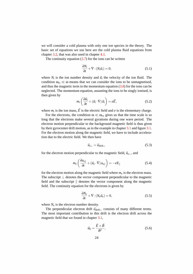
The possible waves for a Gaussian density depletion (see Paper V) are shownin figure5.1, where we have usedm = 1, kz = 2×10−4 m−1, fLH = 250 Hz,fce = 11 kHz,∆ = 0.35 anda = 220 m. The coloured areas mark which fre-quencies have non-evanescent wave solutions at each distance to the cavitycenter. A positive frequency in figure5.1 means waves rotating in the right-handed direction with respect to the background magnetic field. Note that thefrequency spectrum is discrete for waves with frequency below the lower hy-brid frequency, and givenkz andm, so the colour in that frequency range onlymeans that it may exist wave solutions there. The LHC radius is marked withρm in the figure and the 1/e-radius of the cavity witha. The parameters usedhere are those of an observed LHC in the Cluster data (see Paper IV and thenext section). It is possible to estimatekz for the LHCs by combining the the-ory with observations from the Freja and Cluster satellites. This estimate also

28

Distance from center of cavity [m]

Freq

uenc

y [H

z]

ρm a

0 200 400 600 800 1000−500

−400

−300

−200

−100

0

100

200

300

400

500

Figure 5.1: Possible waves in a Gaussian density depletion withm = 1, kz =2× 10−4 m−1, fLH = 250 Hz, fce = 11 kHz, ∆ = 0.35 anda =220 m. A positive frequency corresponds to right-handed wavesand a negative frequency to left-handed waves.

gives an estimate of the length of a typical cavity along the magnetic field. InPaper V, we find that the typical length of a lower hybrid cavity is at least 200times larger than the width.

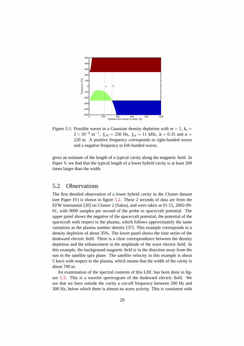
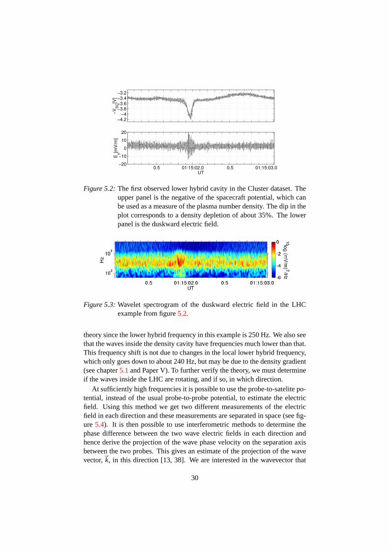
5.2 ObservationsThe first detailed observation of a lower hybrid cavity in the Cluster dataset(see Paper IV) is shown in figure5.2. These 2 seconds of data are from theEFW instrument [20] on Cluster 2 (Salsa), and were taken at 01:15, 2002-09-01, with 9000 samples per second of the probe to spacecraft potential. Theupper panel shows the negative of the spacecraft potential, the potential of thespacecraft with respect to the plasma, which follows approximately the samevariations as the plasma number density [37]. This example corresponds to adensity depletion of about 35%. The lower panel shows the time series of theduskward electric field. There is a clear correspondence between the densitydepletion and the enhancement in the amplitude of the wave electric field. Inthis example, the background magnetic field is in the direction away from thesun in the satellite spin plane. The satellite velocity in this example is about5 km/s with respect to the plasma, which means that the width of the cavity isabout 700 m.

An examination of the spectral contents of this LHC has been done in fig-ure 5.3. This is a wavelet spectrogram of the duskward electric field. Wesee that we have outside the cavity a cut-off frequency between 200 Hz and300 Hz, below which there is almost no wave activity. This is consistent with

29

−4.2−4

−3.8−3.6−3.4−3.2

−V

SC

[V]

0.5 01:15:02.0 0.5 01:15:03.0−20

−10

0

10

20

UT

Ey[m

V/m

]

Figure 5.2: The first observed lower hybrid cavity in the Cluster dataset. Theupper panel is the negative of the spacecraft potential, which canbe used as a measure of the plasma number density. The dip in theplot corresponds to a density depletion of about 35%. The lowerpanel is the duskward electric field.

Figure 5.3: Wavelet spectrogram of the duskward electric field in the LHCexample from figure5.2.

theory since the lower hybrid frequency in this example is 250 Hz. We also seethat the waves inside the density cavity have frequencies much lower than that.This frequency shift is not due to changes in the local lower hybrid frequency,which only goes down to about 240 Hz, but may be due to the density gradient(see chapter5.1and Paper V). To further verify the theory, we must determineif the waves inside the LHC are rotating, and if so, in which direction.

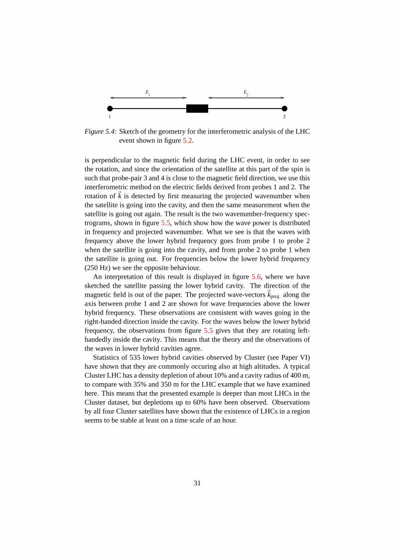
At sufficiently high frequencies it is possible to use the probe-to-satelite po-tential, instead of the usual probe-to-probe potential, to estimate the electricfield. Using this method we get two different measurements of the electricfield in each direction and these measurements are separated in space (see fig-ure 5.4). It is then possible to use interferometric methods to determine thephase difference between the two wave electric fields in each direction andhence derive the projection of the wave phase velocity on the separation axisbetween the two probes. This gives an estimate of the projection of the wavevector,�k, in this direction [13, 38]. We are interested in the wavevector that

30

E2

E1

1 2

Figure 5.4: Sketch of the geometry for the interferometric analysis of the LHCevent shown in figure5.2.

is perpendicular to the magnetic field during the LHC event, in order to seethe rotation, and since the orientation of the satellite at this part of the spin issuch that probe-pair 3 and 4 is close to the magnetic field direction, we use thisinterferometric method on the electric fields derived from probes 1 and 2. Therotation of�k is detected by first measuring the projected wavenumber whenthe satellite is going into the cavity, and then the same measurement when thesatellite is going out again. The result is the two wavenumber-frequency spec-trograms, shown in figure5.5, which show how the wave power is distributedin frequency and projected wavenumber. What we see is that the waves withfrequency above the lower hybrid frequency goes from probe 1 to probe 2when the satellite is going into the cavity, and from probe 2 to probe 1 whenthe satellite is going out. For frequencies below the lower hybrid frequency(250 Hz) we see the opposite behaviour.

An interpretation of this result is displayed in figure5.6, where we havesketched the satellite passing the lower hybrid cavity. The direction of themagnetic field is out of the paper. The projected wave-vectors�kproj. along theaxis between probe 1 and 2 are shown for wave frequencies above the lowerhybrid frequency. These observations are consistent with waves going in theright-handed direction inside the cavity. For the waves below the lower hybridfrequency, the observations from figure5.5 gives that they are rotating left-handedly inside the cavity. This means that the theory and the observations ofthe waves in lower hybrid cavities agree.

Statistics of 535 lower hybrid cavities observed by Cluster (see Paper VI)have shown that they are commonly occuring also at high altitudes. A typicalCluster LHC has a density depletion of about 10% and a cavity radius of 400 m,to compare with 35% and 350 m for the LHC example that we have examinedhere. This means that the presented example is deeper than most LHCs in theCluster dataset, but depletions up to 60% have been observed. Observationsby all four Cluster satellites have shown that the existence of LHCs in a regionseems to be stable at least on a time scale of an hour.

31

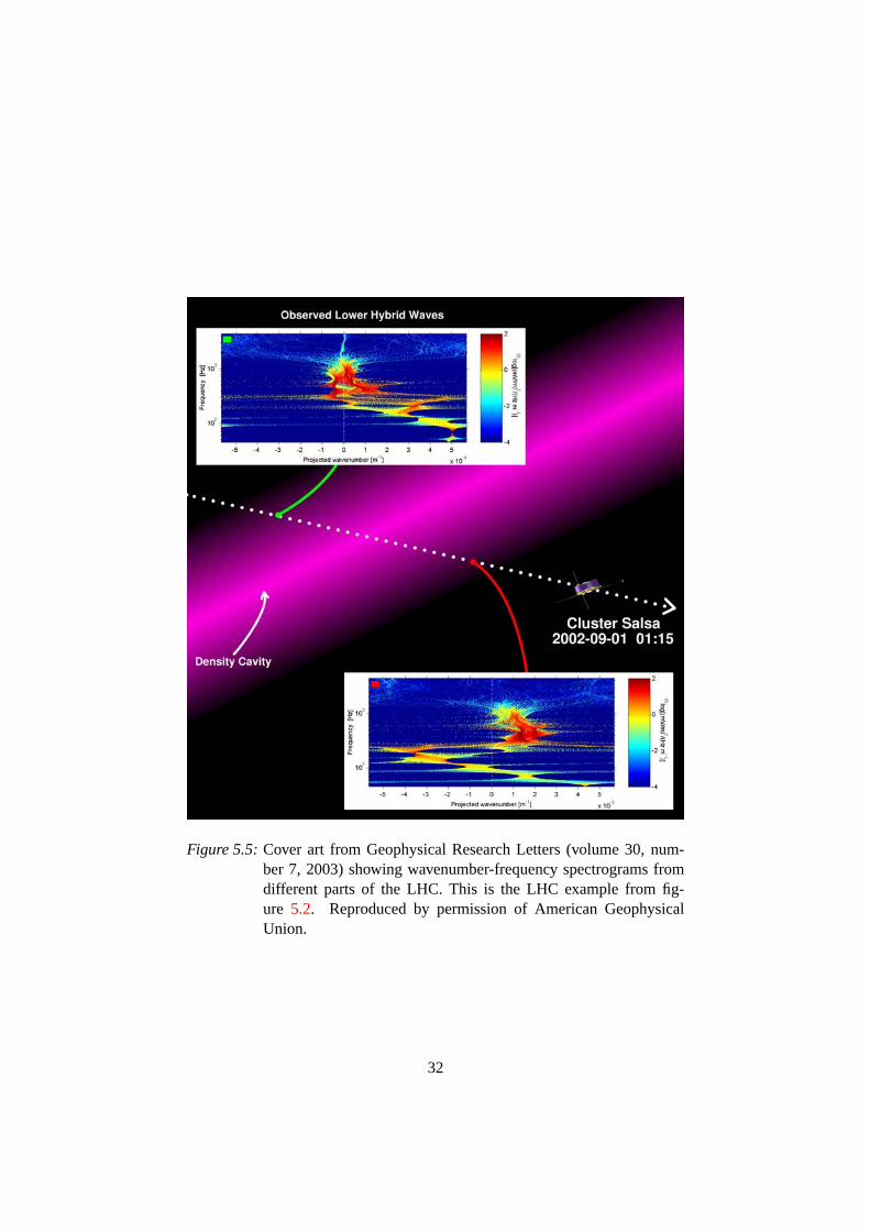
Figure 5.5: Cover art from Geophysical Research Letters (volume 30, num-ber 7, 2003) showing wavenumber-frequency spectrograms fromdifferent parts of the LHC. This is the LHC example from fig-ure 5.2. Reproduced by permission of American GeophysicalUnion.

32

Lower Hybrid Cavity

21

k

B

21

k

kproj.

proj.

Figure 5.6: Sketch of the geometry of the LHC. The direction of the projectedwave-vectors indicated in this sketch are those for wave frequen-cies above the lower hybrid frequency.

33

6 Simple-pole distribution functions

“Why,” he said, “were all the ship’s computations being done on a waiter’s billpad?”

Slartibartfast said, “Because in space travel all the numbers are awful.”He could tell that he wasn’t getting his point across.

From the novel “Life, the Universe and Everything” by Douglas Adams (1982)

Often when investigating plasma properties using kinetic theory, the plasma isassumed to be in thermal equilibrium, that is the particle distribution functionis assumed to be a Maxwellian distributionf (v) ∼ exp(−v2/v2

th). This is notalways a good approach partly because many plasmas, at least in space, are es-sentially collisionless and have no means to rapidly attain thermal equilibrium,partly because the equations for the Maxwellian plasma tend to be complicatedand involve integrals that are not possible to calculate analytically. Thesimple-pole distribution functions that are presented here is an approach that solvesthese problems. The high velocity tail in the particle distribution function of aspace plasma is usually better described with a simple-pole distribution func-tion than by a sum of Maxwellians. The dispersion relations derived for asimple-pole plasma can be used numerically, and sometimes analytically, todescribe and understand the wave properties of a more realistic space plasmathan can be done with a Maxwellian description. The following is a shortintroduction to simple-pole distribution functions with several examples.

6.1 The basic ideaWe saw in chapter4.1 that the dispersion relation for electrostatic waves in anunmagnetised plasma can be written

1−∑α

ω2peα

nα0

Z ∞

−∞

fα0(v)(ω− kv)2 dv = 0, (6.1)

where the summation is made over all particle species in the plasma. The pathof integration is understood to be along the real axis, except that it alwaysgoes below the pole inv = ω/k, even in the case where Im(ω/k) < 0. Letus for convenience only consider high frequency waves so that we only need

35

v

v−∞ ∞

A. B. v

v−∞ ∞

∞∞−i −i

Im

Re Re

Im

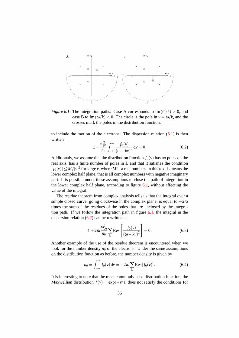
Figure 6.1: The integration paths. Case A corresponds to Im(ω/k) > 0, andcase B to Im(ω/k) < 0. The circle is the pole inv = ω/k, and thecrosses mark the poles in the distribution function.

to include the motion of the electrons. The dispersion relation (6.1) is thenwritten

1− ω2pe

n0

Z ∞

−∞

f0(v)(ω− kv)2 dv = 0, (6.2)

Additionaly, we assume that the distribution functionf0(v) has no poles on thereal axis, has a finite number of poles inL and that it satisfies the condition| f0(v)| ≤ M/|v|2 for largev, whereM is a real number. In this textL means thelower complex half plane, that is all complex numbers with negative imaginarypart. It is possible under these assumptions to close the path of integration inthe lower complex half plane, according to figure6.1, without affecting thevalue of the integral.

The residue theorem from complex analysis tells us that the integral over asimple closed curve, going clockwise in the complex plane, is equal to−2πitimes the sum of the residues of the poles that are enclosed by the integra-tion path. If we follow the integration path in figure6.1, the integral in thedispersion relation (6.2) can be rewritten as

1+2πiω2

pe

n0∑L

Res

[f0(v)

(ω− kv)2

]= 0. (6.3)

Another example of the use of the residue theorem is encountered when welook for the number densityn0 of the electrons. Under the same assumptionson the distribution function as before, the number density is given by

n0 =Z ∞

−∞f0(v)dv = −2πi∑

L

Res[ f0(v)] . (6.4)

It is interesting to note that the most commonly used distribution function, theMaxwellian distributionf (v) = exp(−v2), does not satisfy the conditions for

36

our use of the residue theorem because of its behaviour atv = −i∞. We mustuse other methods for evaluating the integrals in a Maxwellian plasma.

The simple-pole distribution functions are functions of the form

f (v) = ∑j

a j

v−b j, (6.5)

where the numbersa j and b j are complex. They were first introduced byLofgren and Gunell [30], and further explored by Tjulin et al. (see Papers I, IIand III) and Gunell and Skiff [18]. Similar ideas have independently been usedby Nakamura and Hoshino [32] in the context of weakly relativistic cyclotronresonances. In general, the simple-pole distribution function will be complex-valued for realv. This is not a good feature for a distribution function that isused to model a real plasma so we need some conditions on thea js and theb jsfor this function to work properly. If we, for example, for each pole atv = b j

with corresponding residuea j have another pole atv = b∗j with residuea∗j ,where the asterisks mean complex conjugation, we get a real-valued functionfor real values ofv. A simple-pole function following this condition generallybehaves asM/|v| for large|v|, so it still does not satisfy all the conditions forthe use of the residue theorem. We note that if the function, in addition to theprevious condition, satisfies

∑j

Rea j = 0, (6.6)

it will also fulfill the condition | f (v)| ≤ M/|v|2 so that it can be used withthe residue theorem. The simple-pole distribution functions we will considerhere will always satisfy these conditions: They are real-valued for realv, andf (v) → 0 sufficiently fast whenv → ±∞. Another condition we may haveon a distribution function is that it is positive for all realv, which is neededfor physical reasons. The mathematical treatment however does not need thisassumption.

With the simple-pole distribution function (6.5) the number density in theplasma is given by

n0 = −2πi ∑b j∈L

a j (6.7)

where the summation is made over allj for which Imb j < 0, and the dispersionrelation (6.3) can be written in a particularly simple form,

1+2πiω2

pe

n0∑

b j∈L

a j

(ω− kb j)2 = 0. (6.8)

This dispersion relation can easily be rewritten as a polynomial equation inω

∏b j∈L

(ω− kb j)2 +2πi

ω2pe

n0∑

b j∈L

[a j ∏

bl∈L, l �= j

(ω− kbl)2

]= 0, (6.9)

37

which can be solved numerically using standard algorithms. Note that theorder of the polynomial is given by the first term in equation (6.9), and itis twice the number of poles that the simple-pole distribution has in the lowercomplex half plane. This number is equal to the total number of poles, becausethe condition of real valuedness off (v) for real v gives us a pole inv = b∗jfor each pole inv = b j. So for eachk there areN solutions to the dispersionrelation whereN is the number of poles in the simple-pole distribution functionand hence there areN wave modes.

We now check the behaviour of the dispersion relation (6.9) for specialvalues ofk. First, whenk → 0, the dispersion relation transforms into

ωN +2πiω2

pe

n0∑

b j∈L

a jωN−2 = ωN−2(ω2−ω2pe

)= 0, (6.10)

where we have used the number density equation (6.7) and thatN is the numberof poles in the simple-pole distribution function. We have solutions atω = 0andω = ±ωpe, and hence we have a wave mode with a low frequency cut-offat ω = ωpe for all simple-pole distribution functions.

In the limit wherek goes to infinity the dispersion relation turns into

∏b j∈L

(ω− kb j)2 = 0, (6.11)

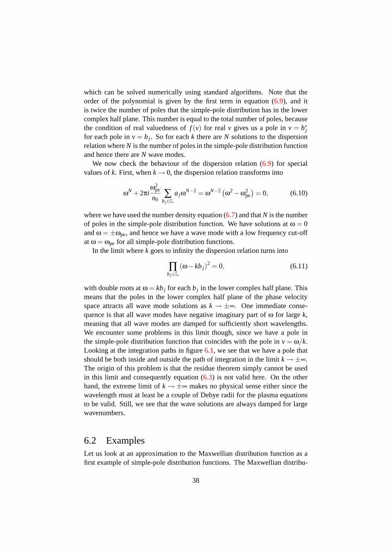
with double roots atω = kb j for eachb j in the lower complex half plane. Thismeans that the poles in the lower complex half plane of the phase velocityspace attracts all wave mode solutions ask → ±∞. One immediate conse-quence is that all wave modes have negative imaginary part ofω for largek,meaning that all wave modes are damped for sufficiently short wavelengths.We encounter some problems in this limit though, since we have a pole inthe simple-pole distribution function that coincides with the pole inv = ω/k.Looking at the integration paths in figure6.1, we see that we have a pole thatshould be both inside and outside the path of integration in the limitk →±∞.The origin of this problem is that the residue theorem simply cannot be usedin this limit and consequently equation (6.3) is not valid here. On the otherhand, the extreme limit ofk → ±∞ makes no physical sense either since thewavelength must at least be a couple of Debye radii for the plasma equationsto be valid. Still, we see that the wave solutions are always damped for largewavenumbers.

6.2 ExamplesLet us look at an approximation to the Maxwellian distribution function as afirst example of simple-pole distribution functions. The Maxwellian distribu-

38

tion fM(v) is given by

fM(v) =n0

vth√

πe−v2/v2

th, (6.12)

wherevth is the thermal velocity of the plasma, defined byvth =√

2kBT/m,wherekB is Boltzmann’s constant,T is the temperature of the plasma andmis the mass of the particles. The most straightforward way to approximate thisexpression with a simple-pole distribution is to truncate the Taylor expansionof the Maxwellian

fM(v) =n0

vth√

πev2/v2th

=n0

vth√

π∑∞m=0

v2m

m!v2mth

≈ n0

vth√

π∑Mm=0

v2m

m!v2mth

. (6.13)

The last expression can be rewritten as a sum of 2M simple poles. ForM ≥ 2,this simple-pole distribution function satisfies the conditions we have set up,and it is always positive for real values ofv so it makes physical sense to usethis expression.

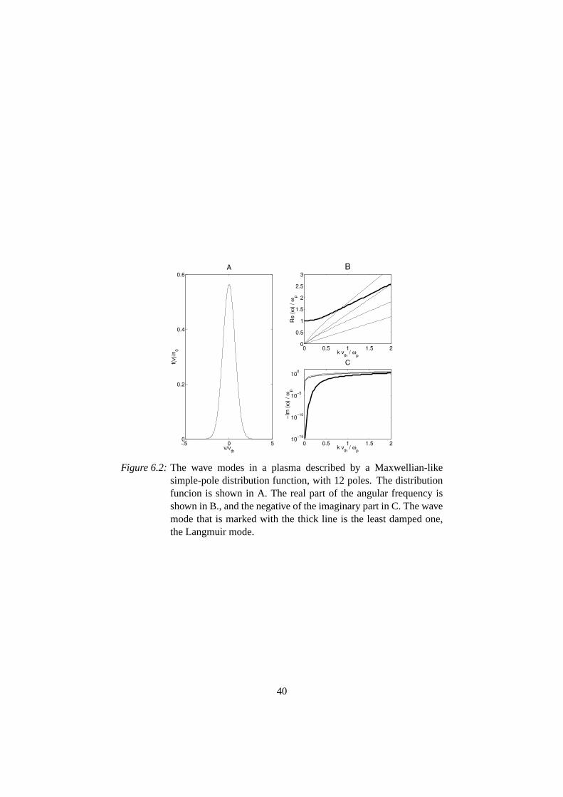
If we use equation (6.13) with M = 6, we get a simple-pole distributionwith 12 poles. We will then find 12 electrostatic wave modes in a plasmamodelled by this distribution function. The wave modes with Reω > 0 areshown in figure6.2. We see that all but one of the wave modes are heavilydamped; have large imaginary part ofω. The lightly damped wave mode isthe Langmuir mode. We may note that the distribution function (6.13) is aneven function, sincefM(−v) = fM(v). The solutions of the dispersion relationfor such functions come in pairs, so that ifω = ωr + iωi is a solution, thenω = −ωr + iωi is another solution. We would thus expect to see six dispersioncurves in figure6.2B, but we only see five. This comes from the fact that thereis a heavily damped solution withωr = 0 that coincides with the horisontalaxis of the plot.

It may be interesting to see what happens when the plasma is drifting withrespect to the observer, or the observer is moving with respect to the plasmarest system. The distribution function is then transformed according tof (v)→f (v− vd), wherevd is the plasma drift velocity. In the case of simple-poledistribution functions (6.5), this means that the polesb j are shifted tob j + vd.This shift will then transform the dispersion relation (6.9) into

∏b j∈L

(ω− kvd− kb j)2 +2πi

ω2pe

n0∑

b j∈L

[a j ∏

bl∈L, l �= j

(ω− kvd− kbl)2

]= 0,

(6.14)where we note that if we writeω0 = ω−kvd, the solutions forω0 are the solu-tions for the unshifted distribution function. We can thus see that the frequen-cies in a drifting plasma is given byω = ω0+kvd, whereω0 is the frequenciesin the stationary plasma. We note that this frequency shift only affects the real

39

−5 0 50

0.2

0.4

0.6

v/vth

f(v)/n

0

A

0 0.5 1 1.5 20

0.5

1

1.5

2

2.5

3

k vth

/ ωp

Re

(ω) /

ωp

B

0 0.5 1 1.5 210

−15

10−10

10−5

100

k vth

/ ωp

−Im

(ω) /

ωp

C

Figure 6.2: The wave modes in a plasma described by a Maxwellian-likesimple-pole distribution function, with 12 poles. The distributionfuncion is shown in A. The real part of the angular frequency isshown in B., and the negative of the imaginary part in C. The wavemode that is marked with the thick line is the least damped one,the Langmuir mode.

40

−5 0 50

0.2

0.4

0.6

v/vth

f(v)/n

0

A

0 0.5 1 1.5 20

0.5

1

1.5

2

k vth

/ ωp

Re

(ω) /

ωp

B

0 0.5 1 1.5 210

−15

10−10

10−5

100

k vth

/ ωp

−Im

(ω) /

ωp

C

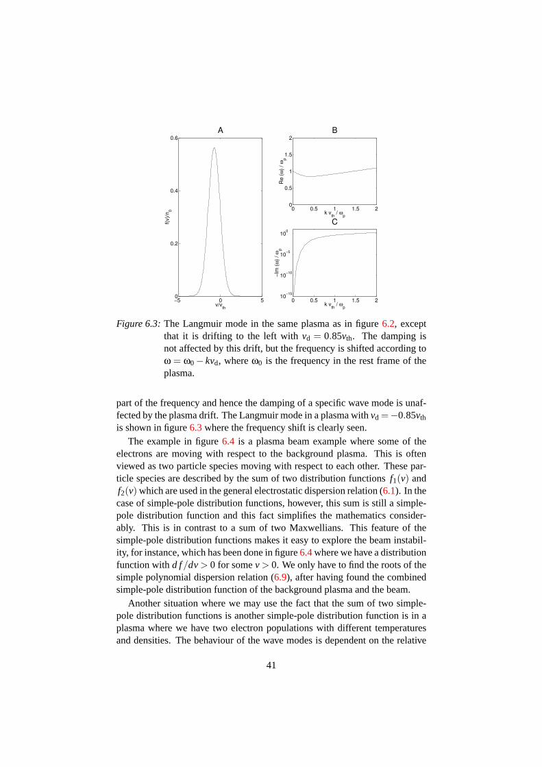
Figure 6.3: The Langmuir mode in the same plasma as in figure6.2, exceptthat it is drifting to the left withvd = 0.85vth. The damping isnot affected by this drift, but the frequency is shifted according toω = ω0− kvd, whereω0 is the frequency in the rest frame of theplasma.

part of the frequency and hence the damping of a specific wave mode is unaf-fected by the plasma drift. The Langmuir mode in a plasma withvd =−0.85vth

is shown in figure6.3where the frequency shift is clearly seen.The example in figure6.4 is a plasma beam example where some of the

electrons are moving with respect to the background plasma. This is oftenviewed as two particle species moving with respect to each other. These par-ticle species are described by the sum of two distribution functionsf1(v) andf2(v) which are used in the general electrostatic dispersion relation (6.1). In thecase of simple-pole distribution functions, however, this sum is still a simple-pole distribution function and this fact simplifies the mathematics consider-ably. This is in contrast to a sum of two Maxwellians. This feature of thesimple-pole distribution functions makes it easy to explore the beam instabil-ity, for instance, which has been done in figure6.4where we have a distributionfunction withd f /dv > 0 for somev > 0. We only have to find the roots of thesimple polynomial dispersion relation (6.9), after having found the combinedsimple-pole distribution function of the background plasma and the beam.

Another situation where we may use the fact that the sum of two simple-pole distribution functions is another simple-pole distribution function is in aplasma where we have two electron populations with different temperaturesand densities. The behaviour of the wave modes is dependent on the relative

41

−5 0 50

0.1

0.2

0.3

0.4

0.5

v/vth

f(v)/n

0

A

0 0.2 0.40

0.2

0.4

0.6

0.8

k vth

/ ωp

Re

(ω) /

ωp

B

0 0.2 0.4−0.02

−0.015

−0.01

−0.005

0

0.005

0.01

k vth

/ ωp

Im (ω

) / ω

p

C

Figure 6.4: The most interesting wave mode in a stationary electron plasmawith a beam with 20% of the background density, the same temper-ature as the background plasma and it is moving atv = 2.2vth withrespect to the background plasma. This wave mode is unstable (hasImω > 0) for values ofk between 0.2ωpe/vth and 0.35ωpe/vth.

density and temperature of the two populations. In figure6.5there is an exam-ple of how a change in the relative density of the electron populations affectsthe wave modes in a plasma where the hot electron temperature is 100 timesthe temperature of the cooler electrons. The solid line is a plasma where thehot electron density is 10% of the cold electron density and for the dashed lineit is 30%. The hot electron population induces damping to the Langmuir wavein both cases, but the Langmuir mode is coupled to the electron acoustic wavemode in the second, but not the first, case. Simple-pole distribution functionsare particularly suited for this kind of parametric investigations.

It is of course also of interest to examine waves at lower frequencies. Weneed then to include the ions in the dispersion relation (6.1). We note that ifwe introduce a generalised distribution functionF0(v), defined by

F0(v) =me

e2 ∑α

q2α

mαfα0(v), (6.15)

whereme is the electron mass,mα is the mass, andqα the charge, of speciesα,the dispersion relation can be written

1− ω2pe

n0

Z ∞

−∞

F0(v)(ω− kv)2 dv = 0. (6.16)

42

−5 0 50

0.2

0.4

0.6

v/vth

f(v)

/n0

A

0 0.1 0.2 0.30

0.5

1

1.5

2

k vth

/ ωp

Re

(ω)

/ ωp

B

0 0.1 0.2 0.3

−0.6

−0.4

−0.2

0

k vth

/ ωp

Im (

ω)

/ ωp

C

Figure 6.5: The least damped wave modes in a plasma with two electron popu-lations of different temperatures. The temperature of the hot elec-trons is 100 times the background plasma temperature, and the hotelectron density is 10% (solid lines) and 30% (dashed lines) of thebackground plasma density. We see that the dispersion curves havedifferent topology in the two cases.

43

−5 0 50

0.1

0.2

0.3

0.4

0.5

0.6

0.7

v/vth

F(v)

/n0

A

0 1 2 3 4 50

0.2

0.4

0.6

0.8

1

1.2

k vth,e

/ ωp,e

Re

(ω) /

ωp,

i

B

0 1 2 3 4 5−0.1

−0.05

0

k vth,e

/ ωp,e

Im (ω

) / ω

p,i

C

Figure 6.6: The ion acoustic wave mode in an electron-hydrogen plasma,where the ion temperature is 1% of the electron temperature. Thegeneralised distribution function in this example is shown in A,where the spike-like feature comes from the ions. This wave modeis very weakly damped for smallk.

Hereωpe denotes the electron plasma frequency andn0 the electron numberdensity. This equation is of exactly the same form as equation (6.2) so if thegeneralised distribution function is a simple-pole distribution, the dispersionrelation is given by equation (6.9). Once again, the fact that a sum of simple-pole distributions is another simple-pole distribution makes it easy to find agood expression for the generalised distribution function. An example with anelectron-hydrogen plasma is shown in figure6.6, where the electron tempera-ture is 100 times the ion temperature.

6.3 Simple-poles in a magnetised plasmaWe will now turn our attention to a three-dimensional homogeneous magne-tised plasma. The dispersion relation for waves in this plasma is given by

det

(k2c2

ω2

(kk− ¯1

)+ ¯ε(�k,ω)

)= 0, (6.17)

where¯ε(�k,ω) is thedielectric tensor [5]. We will here use a coordinate systemwhere the background magnetic field is directed along thez-axis and the wavevector�k is lying in thexz-plane; the so calledStix frame.

44

It is possible to define a three-dimensional gyrotropic simple-pole distribu-tion function as

f (�v) = g(v⊥)h(vz), (6.18)

whereg(v⊥) andh(vz) are simple-pole distribution functions of the same formas before, with

g(v⊥) = ∑j

a j

v⊥−b j(6.19)

andh(vz) = ∑

j

c j

vz −d j. (6.20)

The numbersa j, b j, c j andd j are complex numbers. The dielectric tensor fora plasma described by this distribution function (see Paper III) is given by

εxx = 1+8π2i

ω2k2⊥

∑α

ω2pα ∑

j:bα j∈L

∑k:dαk∈L

aα jcαk

∞

∑n=−∞

n2

× (k2z bα jS1(n,ξα j,Aαk)±Aαkik⊥ωcαS2(n,ξα j,Aαk)

)(6.21)

εxy =4π2

ω2k2⊥

∑α

ω2pα ∑

j:bα j∈L

∑k:dαk∈L

aα jcαk

∞

∑n=−∞

n

× (k2z bα jS3(n,ξα j,Aαk)±2iAαkk⊥ωcαS4(n,ξα j,Aαk)

)(6.22)

εxz =8π2iω2k⊥

∑α

ω2pα ∑

j:bα j∈L

∑k:dαk∈L

aα jcαk

∞

∑n=−∞

n

× ((ω−nωcα)bα jkzS1(n,ξα j,Aαk)± inωgαk⊥dαkS2(n,ξα j,Aαk))

(6.23)

εyy = 1− 8π2iω2 ∑

αω2

pα ∑j:bα j∈L

∑k:dαk∈L

aα jcαk

∞

∑n=−∞

×(

k2z b3

α j

ω2cα

S5(n,ξα j,Aαk)+Aαkbα jS6(n,ξα j,Aαk)

)(6.24)

εyz =4π2

ω2 ∑α

ω2pα

ωcα∑

j:bα j∈L

∑k:dαk∈L

aα jcαk

∞

∑n=−∞

×(

bα jkz (ω−nωcα)k⊥

S3(n,ξα j,Aαk)±2inωcαdαkS4(n,ξα j,Aαk))

(6.25)

εzz = 1+8π2iω2 ∑

α

ω2pα

ω2cα

∑j:bα j∈L

∑k:dαk∈L

aα jcαk

∞

∑n=−∞

×(

bα j (ω−nωcα)2 S1(n,ξα j,Aαk)± inωcαk⊥d2αkS2(n,ξα j,Aαk)

), (6.26)

with εyx = −εxy, εzx = εxz andεzy = −εyz. The gyrofrequencyωcα is in theseexpressions defined so that it is negative for negatively charged particles. In the

45

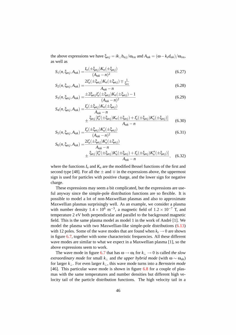
the above expressions we haveξα j = ik⊥bα j/ωcα andAαk = (ω−kzdαk)/ωcα,as well as

S1(n,ξα j,Aαk) =In(±ξα j)Kn(±ξα j)

(Aαk −n)2 (6.27)

S2(n,ξα j,Aαk) =2I′n(±ξα j)Kn(±ξα j)∓ 1

ξα j

Aαk −n(6.28)

S3(n,ξα j,Aαk) =±2ξα jI′n(±ξα j)Kn(±ξα j)−1

(Aαk −n)2 (6.29)

S4(n,ξα j,Aαk) =I′n(±ξα j)Kn(±ξα j)

Aαk −n

± ξα j [I′′n (±ξα j)Kn(±ξα j)+ I′n(±ξα j)K′n(±ξα j)]

Aαk −n(6.30)

S5(n,ξα j,Aαk) =I′n(±ξα j)K′

n(±ξα j)(Aαk −n)2 (6.31)

S6(n,ξα j,Aαk) =2I′n(±ξα j)K′

n(±ξα j)Aαk −n

± ξα j [I′′n (±ξα j)K′n(±ξα j)+ I′n(±ξα j)K′′

n (±ξα j)]Aαk −n

, (6.32)

where the functionsIn andKn are the modified Bessel functions of the first andsecond type [48]. For all the± and∓ in the expressions above, the uppermostsign is used for particles with positive charge, and the lower sign for negativecharge.

These expressions may seem a bit complicated, but the expressions are use-ful anyway since the simple-pole distribution functions are so flexible. It ispossible to model a lot of non-Maxwellian plasmas and also to approximateMaxwellian plasmas surprisingly well. As an example, we consider a plasmawith number density 1.4× 106 m−3, a magnetic field of 1.2× 10−7 T, andtemperature 2 eV both perpendicular and parallel to the background magneticfield. This is the same plasma model as model 1 in the work of Andre [1]. Wemodel the plasma with two Maxwellian-like simple-pole distributions (6.13)with 12 poles. Some of the wave modes that are found whenkz → 0 are shownin figure6.7, together with some characteristic frequencies. All these differentwave modes are similar to what we expect in a Maxwellian plasma [1], so theabove expressions seem to work.

The wave mode in figure6.7 that hasω → ωl for k⊥ → 0 is calledthe slowextraordinary mode for small k⊥ and the upper hybrid mode (with ω ∼ ωuh)for largerk⊥. For even largerk⊥, this wave mode turns into aBernstein mode[46]. This particular wave mode is shown in figure6.8 for a couple of plas-mas with the same temperatures and number densities but different high ve-locity tail of the particle distribution functions. The high velocity tail in a

46

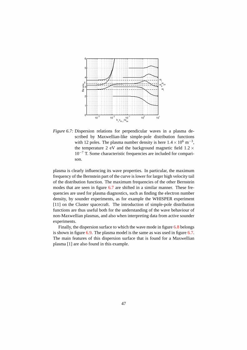
10−3

10−2

10−1

100

101

0

1

2

3

4

5

6

k⊥v

th,⊥/ω

ce

Re

ω/ω

ce ωuh

ωr

ωl

ωp

Figure 6.7: Dispersion relations for perpendicular waves in a plasma de-scribed by Maxwellian-like simple-pole distribution functionswith 12 poles. The plasma number density is here 1.4×106 m−3,the temperature 2 eV and the background magnetic field 1.2×10−7 T. Some characteristic frequencies are included for compari-son.

plasma is clearly influencing its wave properties. In particular, the maximumfrequency of the Bernstein part of the curve is lower for larger high velocity tailof the distribution function. The maximum frequencies of the other Bernsteinmodes that are seen in figure6.7 are shifted in a similar manner. These fre-quencies are used for plasma diagnostics, such as finding the electron numberdensity, by sounder experiments, as for example the WHISPER experiment[11] on the Cluster spacecraft. The introduction of simple-pole distributionfunctions are thus useful both for the understanding of the wave behaviour ofnon-Maxwellian plasmas, and also when interpreting data from active sounderexperiments.

Finally, the dispersion surface to which the wave mode in figure6.8belongsis shown in figure6.9. The plasma model is the same as was used in figure6.7.The main features of this dispersion surface that is found for a Maxwellianplasma [1] are also found in this example.

47

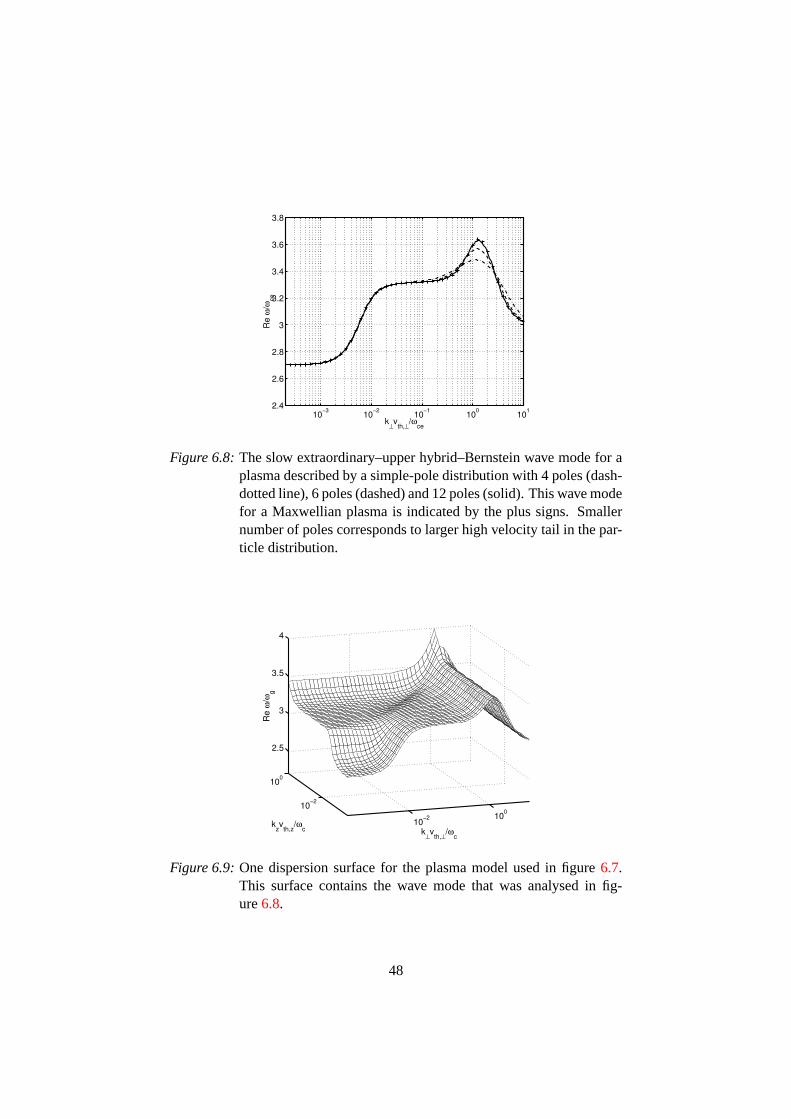
10−3

10−2

10−1

100

101

2.4

2.6

2.8

3

3.2

3.4

3.6

3.8

k⊥v

th,⊥/ω

ce

Re

ω/ω

ce

Figure 6.8: The slow extraordinary–upper hybrid–Bernstein wave mode for aplasma described by a simple-pole distribution with 4 poles (dash-dotted line), 6 poles (dashed) and 12 poles (solid). This wave modefor a Maxwellian plasma is indicated by the plus signs. Smallernumber of poles corresponds to larger high velocity tail in the par-ticle distribution.

10−2 10

010

−2

100

2.5

3

3.5

4

k⊥v

th,⊥/ω

c

kzv

th,z/ω

c

Re

ω/ω

g

Figure 6.9: One dispersion surface for the plasma model used in figure6.7.This surface contains the wave mode that was analysed in fig-ure6.8.

48

7 Future work

As logic stands you couldn’t meet a man who’s from the future.But logic broke as he appeared he spoke about the future.

From the song “All we have is now” by the Flaming Lips (2002)

Most of the work in this thesis has followed two particular paths in the explo-ration of the jungle of space plasma wave phenomena. Observations of lowerhybrid cavities (LHCs) have been combined with the theory of electrostaticwaves in a cold and inhomogeneous plasma, and the electromagnetic waveproperties in a homogeneous plasma described by simple-pole particle distri-bution functions have been investigated. There are still parts of these two pathsthat would be interesting to explore further.

In order to fully understand the waves inside an LHC, it would be usefulto derive the wave properties in a density depletion using the full electromag-netic theory and include thermal effects. Other issues are that it is not clearhow the LHCs are formed, and whether the LHCs are important for the largescale properties, such as particle energisation, of space plasmas. More obser-vations are needed: Both detailed observations of individual LHCs, in orderto compare with theoretical results of their behaviour, and observations of theexistence of LHCs in other parts of space than where they have currently beenfound. It would be interesting to see if it is common for all space plasmasto organise themselves into LHCs, or if the existence of LHCs in the Earth’smagnetosphere and ionosphere is an exception to the general situation.

The simple-pole distributions may be combined with observations in sev-eral ways in order to investigate realistic space plasmas, that is, plasmas not inthermal equilibrium. It is possible to use active sounder measurements of waveresonances in a plasma to estimate the high velocity tail of the electron distri-bution, using results from the theory of simple-pole distributions. The particledistribution in the plasma can then be modelled using only a small numberof parameters, in order to enable further predictions of the behaviour of theplasma. In addition, it is also possible to fit a particle distribution measured byparticle instruments with a simple-pole distribution function and hence derivethe expected wave properties of the plasma, for example the wave resonancesthat are used by sounder instruments.

49

8 Summary of the Papers

Don’t think I can fit it on the paperDon’t think I can get it on the paper

Go ahead and rip up, rip up the paperGo ahead and tear up, tear up the paper

From the song “Paper” by Talking Heads (1979)

Paper I: Using simple-pole distribution functions for calculationsin kinetic theory of plasma wavesThe simple-pole particle distribution function in an unmagnetised plasma isintroduced in this paper. This distribution function is flexible which makes itpossible to use in modelling several different types of plasmas. It also sim-plifies the calculations, compared to the Maxwellian particle distribution, inkinetic plasma theory. The moments of the distribution function, for exam-ple, turn into sums over the poles and the unmagnetised electrostatic disper-sion relation turns into a polynomial equation when a simple-pole distributionfunction is used.

Paper II: Physical interpretation of the Pade approximation of theplasma dispersion functionIn kinetic plasma theory the dispersion relations for a plasma in thermal equi-librium often involves the plasma dispersion funcion,Z, or some related in-tegral function. This function is often calculated numerically using a Padeapproximation. This Pade approximant is in this paper shown to be the exactresult for the dispersion relation in a plasma modelled by simple-pole distri-bution functions. One numerical package that is often used to find dispersionrelations in a magnetised plasma isWHAMP, and it is shown here that the Padeapproximant used inWHAMP corresponds to a plasma with a distribution func-tion that is not strictly positive but negative for some intervals. This impliesthat we have a region with positive slope of the distribution function which ex-plains the known fact that there sometimes are instabilities in the results fromWHAMP, also when modelling a plasma in thermal equilibrium. The distribu-tion function thus found is compared with other simple-pole particle distribu-tion functions, that are strictly positive, and it is shown that even though this

51

distribution function is not strictly positive, it nevertheless approximates theMaxwellian well over a large interval of the velocity domain of the distribu-tion function.

Paper III: The dielectric tensor of simple-pole distribution func-tions in magnetized plasmasIn order to find the dispersion relations in a magnetised plasma we need to findthe dielectric tensor. This has been done in this paper, for a plasma describedby a simple-pole particle distribtion function. There are no integrals in the fi-nal result, which makes the expression somewhat simpler than for other, moreoften used, models of particle distribution functions. The resulting dielectrictensor is used in some numerical examples showing that the number of polesin the simple-pole distribution function, that is the extent of the high veloc-ity tail, changes the dispersion relations at short wavelengths. The maximumfrequency of the Bernstein waves is lower for lower number of poles (largerhigh velocity tail) of the distribution function. This frequency shift may influ-ence estimations of the electron number density from sounder experiments onspacecraft.

Paper IV: Lower hybrid cavities in the inner magnetosphereLower hybrid cavities (LHCs) had previously been observed by sounding rock-ets and the Freja satellite at altitudes below 1750 km. An LHC is a localiseddensity depletion with an increased amplitude of waves in the lower hybrid fre-quency range. LHCs from the Viking and Cluster satellites from altitudes upto 23,500 km are presented in this paper. By making a wavenumber-frequencyspectrum we see that the data in the Cluster event are consistent with waves ro-tating right-handedly with respect to the background magnetic field inside thedensity cavity at frequencies above the lower hybrid frequency, similar to ob-servations by sounding rockets. It seems to be more common for space plasmato organise itself into LHCs than has previously been appreciated.

Paper V: Localization of wave fields in lower hybrid cavitiesThe electrostatic cold plasma theory of lower hybrid waves in a cylindricallysymmetric density depletion is examined in this paper. Inside a depletion witha general density profile, we have waves below the ambient lower hybrid fre-quency with a discrete frequency spectrum, for given value of the parallelwavenumberkz, that are rotating in a left-handed direction with respect to thebackground magnetic field, and waves above the lower hybrid frequency withcontinuous spectrum rotating right-handedly. These results are in agreementwith previous theoretical results for a parabolic density profile. It is found

52

that there is a maximum distance from the cavity center, for a givenkz, withinwhich the waves below the lower hybrid frequency may exist, even though thethe density profile are of essentially infinite extent. There is also a lower limiton the density gradient for these waves to occur. Observations of lower hy-brid cavities (LHCs) can be combined with this theory to get an estimate ofthe maximum possible parallel wavenumber,kz, inside the LHC and hence aminimum value of the cavity length. The examples from the Freja and Clustersatellites show that the length of a typical LHC is at least 200 times its radius.

Paper VI: Observations of lower hybrid cavities in the inner mag-netosphere by the Cluster and Viking satellitesThis paper contains statistics of the lower hybrid cavities (LHCs) that are foundin the datasets from the Viking and Cluster satellites. The LHCs are frequentin the inner magnetosphere and have been found at altitudes up to 35,000 km.166 LHCs were found in total during 27 hours of data on Viking and 535 LHCson Cluster during 87 hours of data. The LHCs are found at invariant latitudesfrom the auroral oval down to the plasmapause. When the occurence frequencyat different altitudes are compared we see that it does not scale with the fluxtube radius, which indicates that the individual LHCs may be long but they donot reach from the ionosphere to 35,000 km altitude. The typical widths ofthe LHCs are found to be between the ion gyro radius and the electromagneticskin depth, and the observed depth of the density depletions varies betweendifferent altitudes. The depth is larger around altitudes of 1000 km (sound-ing rockets, 10–20%), smaller around 1500–13,000 km (Freja and Viking, afew percent) and larger again at 20,000–35,000 km (Cluster, 10–20%). Theobserved LHCs in the inner magnetosphere are situated in a region with back-ground electrostatic hiss in the lower hybrid frequency range, and the existenceof LHCs in a region seem to be stable, at least on a time scale of an hour atCluster altitudes.

53

Acknowledgements

“Suppose you’re thinking about a plate of shrimp. Suddenly someone will say,‘Plate’ or ‘Shrimp’ or ‘Plate of shrimp,’ out of the blue. No explanation and there’s

no point in looking for one either. It’s all part of the cosmic unconsciousness.”

From the film “Repo man” directed by Alex Cox (1984)

There are many people that I would like to thank. The work with this thesiswould have been difficult, boring and probably impossible without them.

First of all, I would like to thank my supervisors Mats Andre and AndersEriksson for all the hours we have spent together trying to understand thedeeper meaning of space and plasma. Anders is responsible for me writingthis thesis. He had a simple idea for a diploma work with simple-pole distri-bution functions that I thought could be interesting. It became clear eventuallythat the project was a bit too large for a six month diploma project, so I had tobecome a PHD student in order to finish the work, which took three years intotal. Mats, on the other hand, is responsible for me finishing the projects, andhe has been encouraging and helpful all the time. It has been fun working withthese two supervisors.

I especially thank the people with whom I have shared office during theseyears: Reine Gill, Mathieu Berthomier and Rico Behlke. The time spent atmy computer would have been much duller without the enlightening and en-tertaining discussions I have had with them.

I also wish to thank Tobias Eriksson, Tobia Carozzi and the other enthusiaststhat have made the ISDAT program working. My research in space would havebeen rather empty without the access to space data. In this context I especiallythank Liza Dackborn for helping me get access to the Viking data and BertilSegerstrom for the computer hardware support.

I wish thank all the people making the Viking and Cluster space missionspossible, particularly those involved in the V2, V4L and V4H instruments onViking and the EFW, STAFF, WHISPER and FGM instruments on Cluster.

Rolf Bostrom, Jan-Ove Hall, Anders Kallstrom, Roger Karlsson, VladimirPavlenko, Kjell Ronnmark, Kristof Stasiewicz, Nico Temme, Bo Thide, An-dris Vaivads and Jan-Erik Wahlund have at times been invaluable when I haveencountered theoretical problems. Their answers have kept me on the righttrack, even though I do not always understand them.

55

My students at the course in Electromagnetic Field Theory the last twospring semesters have been a good help for me trying to understand this elusivesubject. When I tried to explain it to them, I also explained to myself.

I also wish to thank all the other people at IRF-U and the department ofAstronomy and Space Physics that I have not thanked above for their help andhospitality during these years.

Big thanks go to my friends ThomasAgren, Hans Matsson, Mattias En-strom, Lars Eling and all the others. They have continuously showed me thatlife is bigger than space.

Finally I thank my dear mother, father and sister. You have always beenthere for me. I love you.

56

Bibliography

[1] M. Andre. Dispersion surfaces.Journal of Plasma Physics, 33:1–19, 1985.

[2] A. Balogh, M. W. Dunlop, S. W. H. Cowley, D. J. Southwood, J. G. Thomlinson,K. H. Glassmeier, G. Musmann, H. Luhr, S. Buchert, M. H. Acuna, D. H. Fair-field, J. A. Slavin, W. Riedler, K. Schwingenschuh, and M. G. Kivelson. TheCluster magnetic field investigation.Space Science Reviews, 79:65–91, 1997.

[3] W. Baumjohann and R. A. Treumann.Basic space plasma physics. ImperialCollege Press, London, 1996.

[4] M. Born and E. Wolf.Principles of Optics. Pergamon Press, London, 1959.

[5] M. Brambilla. Kinetic theory of plasma waves, homogeneous plasmas.Number 96 in International series of monographs on physics. Oxford UniversityPress, Oxford, 1998.

[6] R. L. Burden and J. D. Faires.Numerical Analysis. PWS Publishing Company,Boston, 5th edition, 1993.

[7] T. D. Carozzi, B. Thide, T. B. Leyser, G. Komrakov, V. Frolov, S. Grach, andE. Sergeev. Full polarimetry measurements of stimulated electromagnetic emis-sions: First results.Journal of Geophysical Research, 106(A10):21395–21407, 2001.

[8] F. F. Chen.Introduction to plasma physics. Plenum Press, New York, 1974.

[9] J. W. Cooley and J. W. Tukey. An algorithm for the machine calculation ofcomplex Fourier series.Mathematics of Computation, 19(90):297–301, 1965.

[10] N. Cornilleau-Wehrlin, P. Chauveau, S. Louis, A. Meyer, J. M. Nappa, S. Per-raut, L. Rezeau, P. Robert, A. Roux, C. de Villedary, Y. de Conchy, L. Friel, C. C.Harvey, D. Hubert, C. Lacombe, R. Manning, F. Wouters, F. Lefeuvre, M. Parrot,J. L. Pincon, B. Poirier, W. Kofman, and P. Louarn. The Cluster spatio-temporalanalysis of field fluctuations (STAFF) experiment.Space Science Reviews,79:107–136, 1997.

57

[11] P. M. E. Decreau, P. Fergeau, V. Krasnosel’skikh, M. Leveque, P. Martin, O. Ran-driamboarison, F. X. Sene, J. G. Trotignon, P. Canu, and P. B. Mogensen. Whis-per, a resonance sounder and wave analyser: Performances and perspectives forthe Cluster mission.Space Science Reviews, 79:157–193, 1997.

[12] P. O. Dovner, A. I. Eriksson, R. Bostrom, B. Holback, J. Waldemark, L. Eliasson,and M. Boehm. The occurence of lower hybrid cavities in the upper ionosphere.Geophysical Research Letters, 24:619–622, 1997.

[13] T. Dudok de Witt, V. V. Krasnosel’skikh, S. D. Bale, M. W. Dunlop, H. Luhr,S. J. Schwartz, and L. J. C. Woolliscroft. Determination of dispersion relationsof quasi-stationary plasma turbulence using dual satellite data.GeophysicalResearch Letters, 22(19):2653–2656, 1995.

[14] A. I. Eriksson. Spectral analysis. In G. Paschmann and P. W. Daly, editors,Analysis methods for multi-spacecraft data, chapter 1, pages 5–42. The In-ternational Space Science Institute, Bern, 1998.

[15] A. I. Eriksson, B. Holback, P. O. Dovner, R. Bostrom, G. Holmgren, M. Andre,L. Eliasson, and P. M. Kintner. Freja observations of correlated small-scale den-sity depletions and enhanced lower hybrid waves.Geophysical Research Let-ters, 21:1843–1846, 1994.

[16] C. P. Escoubet, R. Schmidt, and M. L. Goldstein. Cluster — Science and missionoverview.Space Science Reviews, 79:11–32, 1997.

[17] R. J. Goldston and P. H. Rutherford.Introduction to Plasma Physics. Instituteof Physics Publishing, Bristol, UK, 1995.

[18] H. Gunell and F. Skiff. Weakly damped acoustic-like ion waves in plasmas withnon-Maxwellian ion distributions.Physics of Plasmas, 8(8):3550–3557, 2001.

[19] D. A. Gurnett, R. L. Huff, and D. L. Kirchner. The wide-band plasma waveinvestigation.Space Science Reviews, 79:195–208, 1997.

[20] G. Gustafsson, R. Bostrom, B. Holback, G. Holmgren, A. Lundgren,K. Stasiewicz, L.Ahlen, F. S. Mozer, D. Pankow, P. Harvey, P. Berg, R. Ulrich,A. Pedersen, R. Schmidt, A. Butler, A. W. C. Fransen, D. Klinge, M. Thom-sen, C.-G. Falthammar, P.-A. Lindqvist, S. Christenson, J. Holtet, B. Lybekk,T. A. Sten, P. Tanskanen, K. Lappalainen, and J. Wygant. The electric field andwave experiment for the Cluster mission.Space Science Reviews, 79:137–156,1997.

[21] M. Holschneider.Wavelets — An analysis tool. Oxford Mathematical Mono-graphs. Clarendon Press, Oxford, 1995.

58

[22] S. H. Høymork, H. L. Pecseli, B. Lybekk, J. Trulsen, and A. I. Eriksson. Cavita-tion of lower hybrid waves in the Earth’s ionosphere: A model analysis.Journalof Geophysical Research, 105:18519–18535, 2000.

[23] A. D. Johnstone, C. Alsop, S. Burge, P. J. Carter, A. J. Coates, A. J. Coker, A. N.Fazakerley, M. Grande, R. A. Gowen, C. Gurgiolo, B. K. Hancock, B. Narheim,A. Preece, P. H. Sheather, J. D. Winningham, and R. D. Woodliffe. PEACE: aplasma electron and current experiment.Space Science Reviews, 79:351–398,1997.

[24] M.-B. Kallenrode.Space Physics — An introduction to plasmas and parti-cles in the heliosphere and magnetospheres. Springer, Berlin, 2nd edition,2001.

[25] M. G. Kivelson and C. T. Russel, editors.Introduction to space physics.Cambridge Univeristy Press, Cambridge, 1995.

[26] S. H. Kjus, H. L. Pecseli, B. Lybekk, J. Holtet, J. Trulsen, H. Luhr, and A. Eriks-son. Statistics of the lower hybrid wave cavities detected by the Freja satellite.Journal of Geophysical Research, 103(A11):26633–26647, 1998.

[27] D. J. Knudsen, D. D. Wallis, and H. G. James. Tethered two-point measure-ments of solitary auroral density cavities.Geophysical Research Letters,26(19):2933–2936, 1999.

[28] N. A. Krall and A. W. Trivelpiece.Principles of Plasma Physics. McGraw-Hill, USA, 1973.

[29] J. F. Lemaire and K. I. Gringauz.The Earth’s plasmasphere. Cambridge At-mospheric and Space Science Series. Cambridge University Press, Cambridge,1998.

[30] T. Lofgren and H. Gunell. Flexible simple-pole expansion of distribution func-tions. Physics of Plasmas, 4(10):3469–3476, 1997.

[31] K. A. Lynch, R. L. Arnoldy, P. M. Kintner, P. Schuck, J. W. Bonnell, and V. Cof-fey. Auroral acceleration from lower hybrid solitary structures: A summary ofsounding rocket observations.Journal of Geophysical Research, 104:28515–28534, 1999.

[32] T. K. Nakamura and M. Hoshino. One-over-polynomial approximation for linearkinetic dispersion and its application to relativistic cyclotron resonance.Physicsof Plasmas, 5(10):3547–3551, 1998.

[33] G. Paschmann, F. Melzner, R. Frenzel, H. Vaith, P. Parigger, U. Pagel, O. H.Bauer, G. Haerendel, W. Baumjohann, N. Scopke, R. B. Torbert, B. Briggs,

59

J. Chan, K. Lynch, K. Morey, J. M. Quinn, D. Simpson, C. Young, C. E. McIl-wain, W. Fillius, S. S. Kerr, R. Mahieu, and E. C. Whipple. The electron driftinstrument for Cluster.Space Science Reviews, 79:233–269, 1997.

[34] H. L. Pecseli, K. Iranpour, Ø. Holter, B. Lybekk, J. Holtet, J. Trulsen, A. I.Eriksson, and B. Holback. Lower-hybrid cavities detected by the Freja satellite.Journal of Geophysical Research, 101:5299–5316, 1996.

[35] A. Pedersen. Solar wind and magnetosphere plasma diagnostics by spacecraftelectrostatic potential measurements.Annales Geophysicae, 13(2):118–129,1995.

[36] A. Pedersen, N. Cornilleau-Wehrlin, B. de la Porte, A. Roux, A. Bouabdellah,P. M. E. Decreau, F. Lefeuvre, F. X. Sene, D. Gurnett, R. Huff, G. Gustafsson,G. Holmgren, L. Wooliscroft, H. S. C. Alleyne, J. A. Thompson, and P. H. N.Davies. The wave experiment consortium (WEC).Space Science Reviews,79:93–105, 1997.

[37] A. Pedersen, P. Decreau, C.-P. Escoubet, G. Gustafsson, H. Laakso, P.-A.Lindqvist, B. Lybekk, A. Masson, F. Mozer, and A. Vaivads. Four-point hightime resolution information on electron densities by the electric field experi-ments (EFW) on Cluster.Annales Geophysicae, 19:1483–1489, 2001.

[38] J.-L. Pincon, P. M. Kintner, P. Schuck, and C. E. Seyler. Observation and analy-sis of lower hybrid solitary structures as rotating eigenmodes.Journal of Geo-physical Research, 102:17283–17296, 1997.

[39] H. Reme, J. M. Bosqued, J. A. Sauvaud, A. Cros, J. Dandouras, C. Aoustin,J. Bouyssou, T. Camus, J. Cuvilo, C. Martz, J. L. Medale, H. Perrier, D. Rome-fort, J. Rouzaud, C. d’Uston, E. Mobius, K. Crocker, M. Granoff, L. M. Kistler,M. Popecki, D. Hovestadt, B. Klecker, G. Paschmann, M. Scholer, C. W. Carl-son, D. W. Curtis, R. P. Lin, J. P. McFadden, V. Formisano, E. Amata, M. B.Bavassano-Cattaneo, P. Baldetti, G. Belluci, R. Bruno, G. Chionchio, A. di Lel-lis, E. G. Shelley, A. G. Ghielmetti, W. Lennartsson, A. Korth, H. Rosenbauer,R. Lundin, S. Olsen, G. K. Parks, M. McCarthy, and H. Balsiger. The Cluster ionspectroscopy (CIS) experiment.Space Science Reviews, 79:303–350, 1997.

[40] W. Riedler, K. Torkar, F. Rudenauer, M. Fehringer, A. Pedersen, R. Schmidt,R. J. L. Grard, H. Arends, B. T. Narheim, J. Troim, R. Torbert, R. C. Olsen,E. Whipple, R. Goldstein, N. Valavanoglou, and H. Zhao. Active spacecraftcontrol. Space Science Reviews, 79:271–302, 1997.

[41] K. Ronnmark. Kinetic theory of plasma waves.Space Science Reviews,42:411–428, 1985.

60

[42] P. W. Schuck, J. W. Bonnell, and P. M. Kintner, JR. Lower hybrid solitarystructures.IEEE Transactions on Plasma Science, To be published, 2003.

[43] P. W. Schuck, C. E. Seyler, J.-L. Pinc¸on, J. W. Bonnell, and P. M. Kintner. The-ory, simulation and observation of discrete eigenmodes associated with lowerhybrid solitary structures.Journal of Geophysical Research, 103:6935–6053,1998.

[44] G. Stenberg, T. Oscarsson, M. Andre, and C. C. Chaston. Investigating data wavedata from the FAST satellite by reconstructing the wave distribution function.Journal of Geophysical Research, 107(A8):1190, oi:10.1029/2001JA900154,2002.

[45] T. H. Stix. Waves in space plasmas. American Institute of Physics, New York,1992.

[46] D. G. Swanson.Plasma Waves. Academic Press, New York, 1989.

[47] J. L. Vago, P. M. Kintner, S. W. Chesney, R. L. Arnoly, K. A. Lynch, T. E.Moore, and C. J. Pollock. Transverse ion acceleration by localized lower hybridwaves in the topside auroral ionosphere.Journal of Geophysical Research,97:16935–16957, 1992.

[48] G. N. Watson. A Treatise on the theory of Bessel functions. CambridgeUniversity Press, Cambridge, 2nd edition, 1944.

[49] B. Wilken, W. I. Axford, I. Daglis, P. Daly, W. Guttler, W. H. Ip, A. Korth,G. Kremser, S. Livi, V. M. Vasyliunas, J. Woch, D. Baker, R. D. Belian, J. B.Blake, J. F. Fennell, L. R. Lyons, H. Borg, T. A. Fritz, F. Gliem, R. Rathje,M. Grande, D. Hall, K. Kecsuemety, S. Mckenna-Lawlor, K. Mursula, P. Tan-skanen, Z. Pu, I. Sandahl, E. T. Sarris, M. Scholer, M. Schultz, F. Sørass, andS. Ullaland. Rapid — The imaging energetic particle spectrometer on Cluster.Space Science Reviews, 79:399–473, 1997.

[50] L. J. C. Wooliscroft, S. S. C. Alleyne, C. M. Dunford, A. Sumner, J. A. Thomp-son, S. N. Walker, K. H. Yearby, A. Buckley, S. Chapman, and M. P. Gough.The digital wave-processing experiment on Cluster.Space Science Reviews,79:209–231, 1997.

61

Acta Universitatis UpsaliensisComprehensive Summaries of Uppsala Dissertations

from the Faculty of Science and TechnologyEditor: The Dean of the Faculty of Science and Technology

Distribution:Uppsala University Library

Box 510, SE-751 20 Uppsala, Swedenwww.uu.se, [email protected]

ISSN 1104-232XISBN 91-554-5696-0

A doctoral dissertation from the Faculty of Science and Technology, UppsalaUniversity, is usually a summary of a number of papers. A few copies of thecomplete dissertation are kept at major Swedish research libraries, while thesummary alone is distributed internationally through the series ComprehensiveSummaries of Uppsala Dissertations from the Faculty of Science and Technology.(Prior to October, 1993, the series was published under the title “ComprehensiveSummaries of Uppsala Dissertations from the Faculty of Science”.)

Waves in space plasmas

Documents

Transcript of Waves in space plasmas