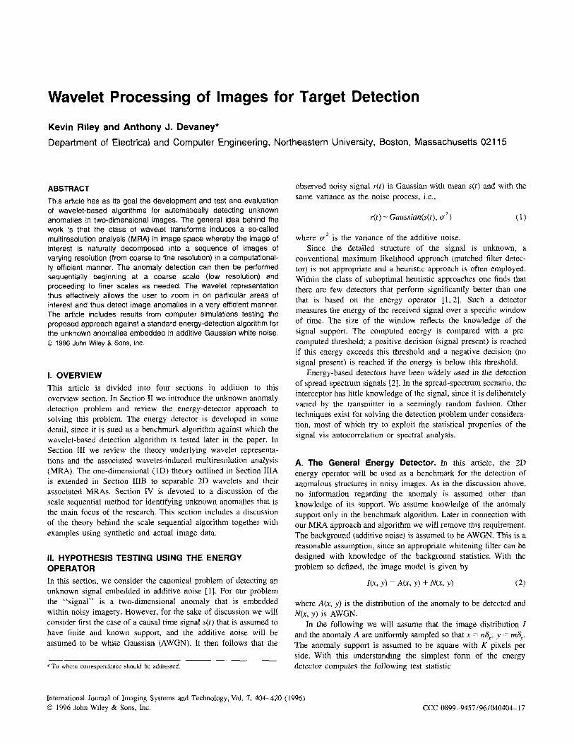
Wavelet Processing of Images for Target Detection

Kevin Riley and Anthony J. Devaney* Department of Electrical and Computer Engineering, Northeastern University, Boston, Massachusetts 021 15

ABSTRACT

This article has as its goal the development and test and evaluation of wavelet-based algorithms for automatically detecting unknown anomalies in two-dimensional images. The general idea behind the work is that the class of wavelet transforms induces a so-called multiresolution analysis (MRA) in image space whereby the image of interest is naturally decomposed into a sequence of images of varying resolution (from coarse to fine resolution) in a computational- ly efficient manner. The anomaly detection can then be performed sequentially beginning at a coarse scale (low resolution) and proceeding to finer scales as needed. The wavelet representation thus effectively allows the user to zoom in on particular areas of interest and thus detect image anomalies in a very efficient manner. The article includes results from computer simulations testing the proposed approach against a standard energy-detection algorithm for the unknown anomalies embedded in additive Gaussian white noise. 0 1996 John Wiley & Sons, Inc.

1. OVERVIEW This article is divided into four sections in addition to this overview section. In Section I1 we introduce the unknown anomaly detection problem and review the energy-detector approach to solving this problem. The energy detector is developed in some detail, since i t is sued as a benchmark algorithm against which the wavelet-based detection algorithm is tested later in the paper. In Section I11 we review the theory underlying wavelet representa- tions and the associated wavelet-induced multiresolution analysis (MRA). The one-dimensional ( ID) theory outlined in Section IIIA is extended in Section IIIB to separable 2D wavelets and their associated MRAs. Section IV is devoted to a discussion of the scale sequential method for identifying unknown anomalies that is the main focus of the research. This section includes a discussion of the theory behind the scale sequential algorithm together with examples using synthetic and actual image data.

II . HYPOTHESIS TESTING USING THE ENERGY OPERATOR In this section, we consider the canonical problem of detecting an unknown signal embedded in additive noise [l]. For our problem the “signal” is a two-dimensional anomaly that is embedded within noisy imagery. However, for the sake of discussion we will consider first the case of a causal time signal s( t ) that is assumed to have finite and known support, and the additive noise will be assumed to be white Gaussian (AWGN). It then follows that the

*To whom correspondence should be addressed.

International Journal of Imaging Systems and Technology, Vol. 7, 404-420 (1996) 0 1996 John Wiley & Sons, Inc.

observed noisy signal r(t) is Gaussian with mean s ( t ) and with the same variance as the noise process, i.e.,

r ( t ) - Gaussian(s(t), a*) (1)

where a* is the variance of the additive noise. Since the detailed structure of the signal is unknown, a

conventional maximum likelihood approach (matched filter detec- tor) is not appropriate and a heuristic approach is often employed. Within the class of suboptimal heuristic approaches one finds that there are few detectors that perform significantly better than one that is based on the energy operator [ I , 21. Such a detector measures the energy of the received signal over a specific window of time. The size of the window reflects the knowledge of the signal support. The computed energy is compared with a pre- computed threshold; a positive decision (signal present) is reached if this energy exceeds this threshold and a negative decision (no signal present) is reached if the energy is below this threshold.

Energy-based detectors have been widely used in the detection of spread-spectrum signals [23. In the spread-spectrum scenario, the interceptor has little knowledge of the signal, since it is deliberately varied by the transmitter in a seemingly random fashion. Other techniques exist for solving the detection problem under considera- tion, most of which try to exploit the statistical properties of the signal via autocorrelation or spectral analysis.

A. The General Energy Detector. In this article, the 2D energy operator will be used as a benchmark for the detection of anomalous structures in noisy images. As in the discussion above, no information regarding the anomaly is assumed other than knowledge of its support. We assume knowledge of the anomaly support only in the benchmark algorithm. Later in connection with our MRA approach and algorithm we will remove this requirement. The background (additive noise) is assumed to be AWGN. This is a reasonable assumption, since an appropriate whitening filter can be designed with knowledge of the background statistics. With the problem so defined, the image model is given by

I(x, Y ) = A(x, Y ) + W , Y ) ( 2 )

where A(x, y) is the distribution of the anomaly to be detected and N(x, y) is AWGN.

In the following we will assume that the image distribution I and the anomaly A are uniformly sampled so that n = nS,, y = m8,. The anomaly support is assumed to be square with K pixels per side. With this understanding the simplest form of the energy detector computes the following test statistic

CCC 0899-9457/96/040404- 17

V(n,rn)= 2 IZ(n ' ,rnl) (3) r i = ) I - K m i ' = m - K

and performs the hypothesis test

H,: V(n, rn) < T anomaly not present

H , : V(n, rn) 2 T anomaly present

where the threshold T is chosen to satisfy a false alarm constraint and the limits of the summation reflect the knowledge of anomaly support. The above test is performed over the entire image which is equivalent to examining the image energy contained in a sliding K X K window. It should be noted that although Equation (3) is defined for a square anomaly, the limits of the summations can be changed to accommodate arbitrary supports. The structure of such a system is shown in Figure 1.

With no knowledge of the anomaly structure, the threshold is chosen to satisfy a false alarm constraint. More specifically, the threshold T is chosen to satisfy the following condition

P,<, = Pr[V(n, rn) 2 T I no anornaZy] (4)

where f,a is the (prespecified) false alarm, rate that the detector is constrained to satisfy. To solve Equation (4) for the threshold T in terms of the preassigned false alarm rate f f u , knowledge of the statistics of V(n, rn) is required. When there is no anomaly present Equations (2) and (3) can be combined to show that the test statistic has the form

V(n,rn) = N*(n' ,rn') ( 5 ) n = , z - K m ' = m - K

where

N(n, rn) - Gaussian(0, u2) . ( 6 )

The test statistic is therefore a sum of squared, independent, and identically distributed Gaussian random variables and, hence, is distributed as a chi-square random variable with N degrees of freedom and scaling factor u2. The degree of freedom N is equal to the number of squared Gaussian random variables that are summed. Such a random variable will be denoted by ,yN. Using this fact, the test statistic in Equation ( 5 ) can be interpreted as the chi-square random variable

( 7 )

With knowledge of the test statistic distribution the false alarm constraint in Equation (4) becomes

where N = K 2 and p,(a) is the aforementioned chi-square dis- tribution. Solutions to Equation (8) have been tabulated and appear in most probability texts.

In summary, if the variance of the AWGN background is known or estimated, a detector based on the energy operator can be constructed to satisfy a false alarm constraint. Such a detector

I h n ) __I Window k-1 ( )2 Threshold+ Decision

requires knowledge of the anomaly support and no other in- formation.

B. Performance Evaluation. The performance of the 2D energy detector will be measured by the probability of detection f d

that is achieved for a given false alarm constraint. The probability of detection is defined as

(9)

Proceeding in the same fashion as in the false alarm calculations, the statistics of V(n, rn) must be obtained. When there is an anomaly present the test statistic has the form of Equation (3), where

f d = f r [V(n, rn) 2 T I anomaly present] .

I(n, rn) - Gaussian(A(n, rn), u2) . (10)

The test statistic is therefore a sum of squared, independent, Gaussian, random variables that have identical variances and means equal to A(n, m). It is well known that such a quantity is distributed as a noncentral chi-square random variable with N degrees of freedom and noncentrality parameter A. Such a random variable will be denoted by ,yN( A). The parameter N is the number of squared Gaussian random variables that are summed, and A is the total anomaly energy. We thus conclude that the test statistic can be interpreted as the noncentral chi-square random variable

where E denotes the anomaly energy.

of detection defined in Equation (9) becomes With knowledge of the test statistic distribution, the probability

'd = ITm PN,E(') da (12)

where N = K 2 and pN,€(a) is the aforementioned noncentral chi- square distribution. In contrast to the chi-square distribution, the values for the non-central chi-square distribution are not well tabulated and an approximation is needed to evaluate Equation ( 12). In this article we approximately convert the non-central chi-square random variable into a chi-square random variable using a relatively simple mapping. If the noncentral chi-square random variable has N degrees of freedom and noncentrality parameter A, define a modified number of degrees of freedom (0) and a threshold divisor (G) as

(N + A)* D=- N + 2 h

N + 2 A G=- N + A

such that

Applying the above approximation to Equations ( 1 1) and (12) yields the following approximated distribution for the test statistic

V(n, rn) - x: and the following expression for the probability of detection

Figure 1. The simple energy detector. where

Vol. 7, 404-420 (1996) 405

(14) and (15) has been compared to the actual performance of a 2D energy detector for several anomaly structures. In particular, the following three anomalies were used: 2 X 2 block with amplitude = 1; 4 X 4 block with amplitude = 112; and 8 X 8 block with amplitude = 114. Each anomaly was embedded in AWGN and the test statistic in Equation (3) was computed over the appropriate support. The test statistic was compared to a threshold which was computed using Equation (8). For each of the three tests, the false alarm constraint was Pfo = 0.001. The graphs comparing the actual energy detector performance to the approximation are shown in

(k2 + EU)’ k 2 + 2E,

k Z + 2Ea k Z + E , ’

D =

(I5)

The above expression for the probability of detection can be readily computed with knowledge of the anomaly support and energy.

The approximation to the probability of detection in Equations

G=-

s? 0 n 0.4

0.2

2x2 Anomaly Stucture 2x2 Anomaly Stucture

x=approx

o=actual

I I I I I I 1 0.1 0.2 0.3 0.4 0.5 0.6 0.7 0.8

STD of AWGN

0’

4x4 Anomaly Stucture

0.1 0.2 0.3 0.4 0.5 0.6 0.7 0.8 STD of AWGN

8x8 Anomaly Stucture

0.1 0.2 0.3 0.4 0.5 0.6 0.7 0.8 STD of AWGN

Figure 2. Comparison of the actual and approximated Pd for the energy detector.

406 Vol. 7, 404-420 (1996)

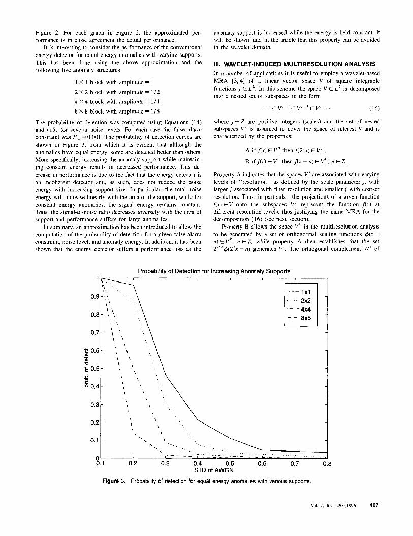
Figure 2. For each graph in Figure 2, the approximated per- formance is in close agreement the actual performance.

It is interesting to consider the performance of the conventional energy detector for equal energy anomalies with varying supports. This has been done using the above approximation and the following five anomaly structures

1 X 1 block with amplitude = 1 2 X 2 block with amplitude = 1 / 2 4 X 4 block with amplitude = 1 /4 8 X 8 block with amplitude = 118.

The probability of detection was computed using Equations (14) and (15) for several noise levels. For each case the false alarm constraint was Pfa = 0.001. The probability of detection curves are shown in Figure 3, from which it is evident that although the anomalies have equal energy, some are detected better than others. More specifically, increasing the anomaly support while maintain- ing constant energy results in decreased performance. This de- crease in performance is due to the fact that the energy detector is an incoherent detector and, as such, does not reduce the noise energy with increasing support size. In particular, the total noise energy will increase linearly with the area of the support, while for constant energy anomalies, the signal energy remains constant. Thus, the signal-to-noise ratio decreases inversely with the area of support and performance suffers for large anomalies.

In summary, an approximation has been introduced to allow the computation of the probability of detection for a given false alarm constraint, noise level, and anomaly energy. In addition, it has been shown that the energy detector suffers a performance loss as the

1

0.9

0.8

0.7

$j 0.6

% 0.5 d g a 0.4

- al -0

0.3

0.2

0.1

0 C

anomaly support is increased while the energy is held constant. It will be shown later in the article that this property can be avoided in the wavelet domain.

111. WAVELET-INDUCED MULTIRESOLUTION ANALYSIS In a number of applications it is useful to employ a wavelet-based MRA [3,4] of a linear vector space V of square integrable functions f E L2. In this scheme the space V C L2 is decomposed into a nested set of subspaces in the form

. . . . . . (16)

where j E Z are positive integers (scales) and the set of nested subspaces V’ is assumed to cover the space of interest V and is characterized by the properties:

c v1-2 c v’- ’ c V’

A if f(x) E V” then f( 2 ’x) E V’ ;

B if f(x) E V” then f ( x - n) E V”, n E Z

Property A indicates that the spaces V’ are associated with varying levels of “resolution” as defined by the scale parameter j , with larger j associated with finer resolution and smaller j with coarser resolution. Thus, in particular, the projections of a given function f ( x ) E V onto the subspaces V’ represent the function f ( x ) at different resolution levels, thus justifying the name MRA for the decomposition (16) (see next section).

Property B allows the space V” in the multiresolution analysis to be generated by a set of orthonormal scaling functions +(x - n) E V”, n EZ, while property A then establishes that the set 2’”+(2’x - n) generates V’. The orthogonal complement W’ of

Probability of Detection for Increasing Anomaly Supports

\ \ \

\ \ ....... ‘ ’\

\ ’\

\ \ \. ........

\ ’ \ \.

. . . . .

’ - ’ - 4x4 8x8 El - -

\

\ . . . . . . . . . . . . . . . . . . . . . . . . . . . . . . . . . . . . . . . . . . . . . . - . -.-.-.-.-I-.-.-.-.L.-.- - . - . - . ‘.

y - - - - + - - - - - \

I ~~

0.2 0.3 0.4 0.5 0.6 0.7 0.8 STD of AWGN

Figure 3. Probability of detection for equal energy anomalies with various supports.

Vol. 7, 404-420 (1996) 407

the space V’ with respect to the next higher resolution space V’+’; I.e.,

(17) is called the j t h wavelet space and is generated by an orthonormal set of wavelets 2’”$(2’t - n) [3,4]. The wavelet spaces W’, j E 2 are nonoverlapping and completely cover the space V so that a decomposition of a functionf(x) E V into the wavelet spaces (via a wavelet expansion) corresponds to a decomposition of this function into orthogonal components at different resolution levels. This last property makes the MRA extremely attractive in a number of signal-processing applications [3].

The above ideas readily generalize to more that one dimension. In particular, for a linear vector space of functions of N variables f(r) , r={x . , , x , , . . . , x N } E R N we have the MRA defined by Equation (16) where the subspaces V’ are now N-dimensional and can be decomposed into the tensor product of N 1D spaces V:, 1 = 1,2, . . . , N according to the equation

V’ + ’ = V’ @ W’

V’ = V” CQv; 8 . . -v ; , (18)

and where the wavelet spaces W’ are still defined according to Equation ( 1 7). This “separable” MRA is generated by a scaling function which is equal to the product of N 1D scaling functions

N

= 2”” 4(2Jx, - n , ) , (19) I = I

where n = {n , , n2, . . . , n,}. The wavelet spaces are generated by 2N - 1 mutually orthogonal wavelets formed from all possible N-tuple products of 1D scaling functions and wavelets [4]. For example, in 2D ( N = 2) there are three mutually orthogonal wavelets given by

jth scale approximation of f(x) [as defined by Eq. (24)] and play the same role for functionsf’ E V’ as do the sample valuesf’(nS,) for functionsf’(x) bandlimited to the pass band [ - d S , , +dS,]. Indeed, it is readily verified that the choice +(x) = sin(m)/at = Sinc(x) generates the spaces V’ corresponding to bandlimited functions having Nyquist sampling intervals S, = 1 /2’, so that for this choice a: =f’(nS,) and the expansion Equation (24) reduces to the Whittaker Shannon expansion. Other choices of scaling functions 4(x ) then lead to more general sets of scaling coefficients and a more general interpretation of “sample value” and “res- olution.”

That the scaling coefficients al, can be interpreted as general- ized Nyquist samples is reinforced by the fact that the expression for the jth scale sampling coefficients a’, given in Equation (25) can be interpreted as convolution followed by discrete sampling at the “Nyquist rate” r = I /S, = 2’. In particular, we may write this equation in the form

where 8 denotes the convolution operation. Thus, the scaling coefficients are interpreted as being the sampled output of the low-pass filter 4i(-x) in complete analogy to the interpretation of the conventional Nyquist samples as being the output of an ideal low-pass filter.

As discussed in Section 111, the difference between two adjacent resolution spaces V’+’ and V’ is the wavelet space W’; i.e., V’” = V’@ W’. The wavelet space W’ is spanned by the set of orthonormal functions $:(x) = 2”’$(2’x ~ n), where $(x) is a wavelet that, like the scaling function, is orthonormal under integer translations. In addition, because the wavelet space W’ is the orthogonal complement of V’ relative to V J + ’ , the functions 4; and $’,. are orthogonal for all n, n‘ E Z and j s j ’ €2. The functionf(x) has a projection onto W’ given by

r

W f ’ W = c b:$’,(x) (27) n - x

A. Wavelet Theory. We consider the set of orthonormal func- tions ~$’,(x) = 2’/’4(2’x - n) where j, n are integers and 4 ( x ) is a (real valued) scaling function [3,4] that is orthonormal under integer translations; i.e.,

are the wavelet coefficients (or wavelet transform) of the function f(x) at the scale j.

Since V’+’ =V’@W’ i t follows that the projection of any function f(x) onto the j t h resolution space V’ can be decomposed into the sum of the projections onto the orthogonal subspaces V’-‘

(23) and W / - ’ so that

where = 1 if n = 0 and zero otherwise is the Kronecker delta f’(x> = f ’ - ‘ ( x ) + wf’-’(x).

function. As indicated in Section 111, the set of scaling functions @:, are orthonormal with respect to n because of Equation (23) and span the j t h resolution space V’ in the MRA of linear vector spaces V of square integrable functions f E L’. A function f(x) E V has a projection onto V’ given by

By substituting the expansions (24) and (27) into Equation (29) and projecting both sides of the resuIting equation onto V’, V’-’, and W’-’, we obtain the following pyramid algorithms relating the discrete representation u’, to a:- I , and 6:- ’:

m u’, = 2 h(n - 2n‘)a:,T’ t 5 g(n - 2n’)b’,T’ (30) n l = - a “ = - m f’b) = c a’ ,4 ’ ,0 (24) m

where

The set of scaling coefficients u:, n E 2 completely specify the where

408 Vol. 7, 404-420 (1996)

three mutually orthogonal wavelets as defined in Equations (20- 22): h(n) = 1 dx +;(x)+;-J(x) = v5 1 dx +(2t - n)+(x) (33)

are the inner products (matrix elements) between the basis func- tions 4; and 4i-I and +;t and $ ; - I , respectively.

The matrix elements h(n) and g(n) are the key defining quantities in wavelet theory [3,4] and in the MRA induced by the scaling functions. These quantities both define the scaling functions and wavelets and also act as discrete filters relating the representa- tions u;, u : ~ - ’ , and b:t-‘ via the pyramid algorithms (30), (31), and (32). In general, for the wavelets @(x) and scaling functions $(x) to be orthogonal under integer translations, these coefficients are related to the equation g(n) = (- l)”h( 1 - n). Various choices exist for the basic set h(n) including the important classes of causal, finite impulse response (FIR) filters that give rise to compactly supported scaling functions and wavelets. Two examples of this latter class of filters are the Haar filters h(0) = h( 1) = 1 /A, and h(n) = 0, otherwise, and Daubechies filters [4] h(0) = 1 /4( 1 + &), h ( l ) = 1/4(3+&), h(2)= 1/4(3-&), h(3)= 1/4(1 -A), and h(n) = 0, otherwise.

We show in Figure 4 a wavelet-based PR filter bank where the input sequence of scaling coefficients a’, at scale j is converted via filtering and decimation to the scaling coefficient a’,- I and wavelet coefficients bi-’ at the next lower scale j - 1. The filtering and decimation operations are defined mathematically by the down- pyramid Equations (31) and (32). The synthesis section of the bank then expands these two sequences and filters them with the filters h(n) and g(n) to regenerate the original sequence a’,. The expansion and filtering operations of the synthesis section of the the filter bank are defined mathematically by the up-pyramid Equations (30).

B. Two-dimensional Wavelet Theory. As indicated in Sec- tion 111, all of the results outlined above generalize to higher dimensions. In particular, for the case of 2D appropriate to image processing we consider a linear vector space of functions of two variables f(x, y), and have the MRA defined by Equation (16), where the subspaces V’ are now 2D. These 2D spaces can be decomposed into the tensor product of two ID spaces, V” and V’,,, according to the equation V’ = V: @ V: and where the wavelet spaces W’ are still defined according to Equation (17). This separable MRA is generated by a scaling function which is equal to the product of two 1D scaling functions

The wavelet spaces are generated by three mutually orthogonal wavelets formed from all possible double products of ID scaling functions and wavelets [3,4]. For example, in 2D (N = 2) there are

$;zl,&> Y; 1) = 4 p $ : * ( Y ) >

$’,,,,,,(x, Y; 2) = $;l(x)4’,z(Y) 3

Y; 3) = $;,(xI$:JY) 1

which generate the three wavelet spaces.

analogy to Equation (24), by A 2D function f(x, y ) E V has a projection onto V’ given, in

f ’k Y ) = c 4,m4’,,m(x> Y ) (36) n.m

where

+’,,Jx, Y) = 2-’4[2’(x - n), 2’(y - m)l

= 2-’+[2’(x - n)1+[2’(y - m)]

with the last equality holding for separable wavelet bases. The scaling coefficients an,m are given by

(37)

As in the ID case, the set of scaling coefficients a’,,, completely specify the jth scale approximation of f(x, y ) [as defined by Eq. (36)], and can be interpreted as generalized (2D) Nyquist samples.

The function f(x, y) has projections onto the three wavelet spaces W’], W;, W< spanned by the three 2D wavelets $’,,,,,,(x, Y; 11, $<tl,f12(x, y ; 21, and $:tl.n2(.x, Y ; 3) given by

wfJ(x, y; 1 ) = c b;,m(w:,m(.x, y; 1 ) (38) n.m

where 1 = 1,2,3, and

b’,JU = 1 dx 4 f(x3 y)$’,.,(x, y; 1 ) . (39)

are the wavelet coefficients (or wavelet transform) of the function f(x, y) at the scale j .

Since V’+’ = V’ CB W’ it follows that the projection of any functionf(x, y) onto the jth resolution space V’ can be decomposed into the sum of the projections onto the orthogonal subspaces V’-’ and wj-1 = w:-l @wW.,-l @w;-I so that

f’(x, y) = f ’ - ’ ( x , y) + wf’-’(x, y ; 1) + wf’-’(x, y ; 2)

+ wf’-l(x, y; 3) . (40)

By substituting the expansions (36) and (38) into Equation (40) and projecting both sides of the resulting equation onto V’, V’-’, and W’-’(l), 1 = 1,2,3, it is possible to obtain pyramid algorithms analogous to Equations (30)-(32). However, for the purposes of this report we will need only the scaling function down pyramid,

{TTEai-z-ZTZ 4 4

d - n ) G- 2 r Figure 4. The analysis and synthesis sections of a wavelet-based PR filter bank.

Vol. 7, 404-420 (1996) 409

which in analogy to Equation (31) is The approach outlined in the paragraph above can be further explained as follows. The first step in the procedure is to decompose the original high resolution (fine scale) image I(x, y) (the “data”) into a set of scaling coefficients a:,, at the finest

a’-’ n.n, = 2 h(n’ - 2n)h(m’ - 2rn)ai,,,n, . (41) 18 ‘ m ’

C. Wavelet Viewing Window. A key property of wavelets and scaling functions is the fact that they are compactly supported. This guarantees that the discrete filters h(n) and g(n) are FIR filters so that the up- and down-pyramid algorithms are exceptionally efficient. More important for anomaly detection is the fact that this implies that the scaling coefficients a :,,,n representing the function f ( x . y) depend and define this function in the immediate vicinity of the space point x = n/2’, y = m/2’. This leads to the concept of a viewing window WinJ@, rn) that is simply the support region of the scaled and displaced scaling function 4[2’(x - n/2’), 2’(y - m / 2’)]. For example, for Haar bases the viewing window is a rectangle whose lower left corner is x = n6, = n/2’ , y = mq = m/ 2’ and whose sides have length equal to 24 = 2’-’. For the Daubechies bases the viewing window is a rectangle whose lower left corner is n6,, mq and whose sides have length equal to 66,. The importance of the viewing window is that it defines the support region over which the scaling coefficient a’,,,m depends. The viewing window plays an important role in anomaly detection as will be shown below.

IV. SCALE SEQUENTIAL ANOMALY DETECTION The wavelet representations that we consider in this article are the classical compactly supported wavelets reviewed in the preceding two sections. We chose this class because of their superior signal processing capabilities that results from the pyramid algorithms Equations (30)-(32) that govern the manipulation of the wavelet coefficients in wavelet space [4]. We can summarize the advantages of compactly supported orthonormal wavelet representations as follows:

The wavelets and scaling functions c $ ’ , ~ , ~ are such that the scaling coefficients u’,,,,, at the different scales are related by FIR filters via pyramid algorithms [cf. Eq. (41)l. The wavelets and scaling functions are compactly supported so that the scaling coefficients represent the image in compactly supported regions of the x, y plane. The sample spacing 8, = 8, = 1 /2’ at any given scale varies with the scale. Another way of saying this is that the filter window vanes with scale unlike other phase space repre- sentations such as the short time Fourier representation and the Gabor representation.

The above advantages are extremely important in automatic target detection and identification, since we require the algorithms to be fast and efficient and to operate in a coarse-to-fine zoom manner.

The actual anomaly detection is performed using a scale sequential energy detector whereby the local image energy is computed at each scale and used to localize the image anomaly at that scale. A key ingredient of the method is to implement the procedure in a scale sequential manner whereby the detection is performed sequentially in a number of steps starting at low resolution (low scale j,) and proceeding sequentially to higher resolution (higher;) and to a final decision step at some finest scale J . This scale sequential procedure minimizes the CPU time required to achieve an anomaly detection with small sacrifice in error.

scale J . This is accomplished using the scaling function representa- tion Equation (36)

where

As discussed in Section 111, the coefficient set a:,rn can be thought of as generalized sample values of the image. In particular, these coefficients correspond to the sampled output of the 2D filter q5&>(-x, -y) at the “Nyquist rate” r = 1 /SJ = 2J. Moreover, it can be shown [4] that for sufficiently large J (very fine scale) the coefficients actually become equal to the conventional Nyquist samples of the image. Thus, for suitably fine sampling we can regard the raw sampled image to be equal to the scaling coefficient

at lower scales j < J can be viewed as generalized sample values of the image at the scale (resolution) j . The greater the scale parameter j , the finer the resolution; and the smaller the value of j , the coarser the resolution. Thus, i t is possible to examine the image at coarser scales; < J by means of the projection of Z(x, y) onto a subspace V’ E V J according to Equation (36); i.e.,

set QL. The scaling coefficients

“ G - 3 Y) = c Q’,t,,,,4’,,.,Jx, Y) (43 ) , , ,m

where now the scaling coefficients a :,,, are generalized sample values of the lower resolution image ZJ(x, y) and are given by Equation (42), with J replaced by J. As discussed in the preceding section the coefficients at lower scales are directly computable in terms of the coefficients at higher scales via the down-pyramid algorithm Equation (41).

A. Wavelet Energy Detection. The problem we address is that of determining the location of an unknown anomaly within a given image I(x, y). Unlike the benchmark energy detector discussed in Section 11, we assume no knowledge whatsoever of the anomaly, not even its support which is assumed known in the standard energy detector. Our approach to this problem is to examine the energy of each scaling coefficient u<~,+, beginning at some coarse scale j,, and proceeding to higher scales j > j l ) until a scale J is reached where the energy begins to decrease. The general motiva- tion for this procedure is that u:,,,,, represents the anomaly within the viewing window WinJ(n, rn) so that if the energy exceeds some threshold then it is probable that the anomaly is localized within this viewing window. The scale sequential procedure than scans the viewing window over the image with the window size varying from some large area 4, (corresponding to the coarse scale j , ) ) to successively smaller areas d,, Sa,, . . . , dK at scales j =

j , , J,, . . . , j,. The location and size of the anomaly is determined by the location and size of the window that maximizes the energy. A precise statement of this strategy together with examples are presented below.

The anomaly detection and identification are performed directly using the scaling coefficients a:, at the different scales. In

410 Vol. 7, 404-420 (1996)

particular, the coarse scale coefficients a?’ are first computed using the down-pyramid algorithm Equation (41) from the fine- scale (original image) coefficients These coefficients are then input into the energy detector and a decision is made at each space point x o = n,/2’”, yo = m,,/21° on whether this space point sam- ples an image anomaly. It is important to note that the generalized sample values at this coarse scale corresponds to the area of the viewing window as represented by the support of the scaling function at that scale. Thus, the decision as to whether any scaling coefficient samples an anomaly is, in fact, equivalent to deciding whether the image within this window contains an anomaly.

The next step is to compute the energy at the next finer scale j o + I over those sets of points in the immediate vicinity of those points x o = n,/2’”, yo = m,,/2’O that tested positive at scale j , ) . The selection of which points to test at the next finer scale is determined by the viewing window that was defined in Section IIIC. In particular, the scaling coefficient u ~ ~ ~ ~ , , , ~ ~ is com- pletely determined by points n, m contained within the window Win,l,(n(,, mo) so that only these latter points need to be tested. Again a decision is made over the new reduced set of points and the process continues to finer scales.

The method outlined above has a number of advantages over alternative nonwavelet-based procedures such as the standard energy detector discussed in Section 11. First, it is extremely fast and efficient owing to the superior signal processing abilities of discrete compactly supported orthonormal wavelets. Second, it enjoys superior signal to noise ratios since decisions are made based on local windows in image space. Thus, extraneous noise from windows not containing image anomalies do not affect the decision strategy in windows containing anomalies. Moreover, since a given coefficient u : ~ , , ~ is related to the image I(x, y ) via a low-pass filter, the additive noise is low-pass filtered, thus directly increasing signal to noise ratio. Finally, the variable zoom window allows for the possibility of using an optimum window size for a wide range of anomaly sizes. This cannot be attained, for example, with the shortime Fourier transform or Gabor representation, which use a fixed window size.

6. Wavelet Anomaly Detection Algorithm. In this section the ideas outlined above are used to develop a detection algorithm for identifying anomalies in 2D images. In particular, a wavelet domain energy detector is introduced which requires no knowledge of the anomaly support or detail. The wavelet-induced MRA provides a means for sequentially zooming in on image areas with significant energy. This approach leads to an efficient algorithm which is capable of quickly processing large images.

The first step in the algorithm is to examine the scaling coefficients at a coarsest scale, j,. As discussed earlier the scaling coefficients at scale j , are derived from a viewing window Win,@ m) so that examining the energy of the coefficient a::wz effectively examines the energy of a low-pass-filtered version of the image detail contained within this window. From this it follows that if the energy la:,”m\2 exceeds a threshold T it is reasonable to suppose that an anomaly resides in the wavelet viewing window. With respect to the conventional energy detector, examining the scaling coefficient energy at scale j , is analogous to computing Equation (3) at scale j , for K = 1.

After examining the scaling coefficients at scale j , and hypoth- esizing possible anomaly locations, the next step in the algorithm is to localize or zoom in on candidate anomalies. This is accom-

plished by examining the energy of the scaling coefficients at scale j , + 1, since these coefficients are derived from smaller viewing windows in the original image, i.e.,

support [,’a+ ‘ (n , m)] <support [W’”(n, m)] . (44)

The selection of which scaling coefficients to test at scale j,, + 1 is performed as follows. Only those points at scale j , + 1 whose viewing windows intersect the viewing windows that tested positive at scale j , are considered. In other words, the coefficients that are tested at scale j , + 1 represent subsets of pixels contained within viewing windows that tested positive at scale j,. Therefore, deciding that a scaling coefficient represents a region containing an anomaly at scale j , , implies that the anomaly is contained in an area smaller or equal to the size of the viewing window at scale j,.

This process proceeds to finer scales, sequentially considering smaller viewing windows and localizing anomaly energy. This idea is further illustrated by the following wavelet domain adaptation of Equation (3)

(u:t.m)2 is analogous to 2 C ~’(n’ ,rn‘)

where j denotes the wavelet scale and K, denotes the size of the viewing window (which decreases as j increases) that the scaling coefficient u : ~ , ~ is derived from. The algorithm will stop trying to localize the anomaly when the energy of the scaling coefficients at scale j ’ + 1 is less than the energy of the corresponding coefficients that tested positive at scale;’. The is equivalent to zooming in too far on the anomaly and the algorithm stops and declares the previous step in the process as the final anomaly location.

With the motivation behind the wavelet-based energy detection algorithm detailed, the specific steps of the algorithm can be presented. These steps are as follows:

( , r ’ .m ’ ) E K,

1.

2.

3.

4.

5 .

Compute the energies of the scaling coefficients at a coarsest wavelet scale and compare to the threshold [analogous to computing Eq. (3) for K large]. In no energies exceed the threshold, repeat step 1 using the next higher wavelet scale which analogous to computing (Equation (3) over a smaller K. Once a scaling coefficient energy exceeds the threshold, mark it is a candidate. Using the next higher wavelet scale, compute the energies of only those scaling coefficients that correspond to the same viewing window in the original image as the candidate pixel (i.e., try to localize the energy identified at the lower resolution). If the energy of any scaling coefficient exceeds the threshold mark these as the new candidates and repeat step 4. If no scaling coefficient energies exceed the threshold the anomaly energy cannot be localized any further. Consequently, the algorithm stops and declares the viewing windows in the original image corresponding to the candidate scaling co- efficients as the anomaly locations.

By sequentially processing only those viewing windows which correspond to candidate pixels, the computational cost of the algorithm is significantly reduced. This provides for a fast decision rate at the expense of a small decrease in detection performance.

I . Threshold Computation. With no knowledge of the anomaly structure, the threshold that the scaling coefficient energy is tested against can only be computed to satisfy a false alarm constraint.

Vol. 7, 404-420 (1996) 411

When there is no anomaly present, the scaling coefficients at scalej are given by

where N i , m represents the wavelet decomposition of the AWGN background in the original image. As mentioned previously, the scaling coefficients of the noise remain white and uncorrelated. In particular,

- Gaussian(0, g’) (46)

where uz is the original noise variance. As a result, the scaling coefficient energy is the square of a Gaussian random variable and therefore distributed as a chi-square random variable with one degree of freedom and scaling factor u2. With knowledge of the pixel energy distribution, a false alarm constraint can be con- structed as

P,o = Pr[(a’,,,)’ > T 1 no anomaly] = JTmp,(a) da

where p , (a) is the aforementioned chi-square distribution. Solutions to the above equation have been tabulated and appear

in most probability texts. In summary, if the variance of the AWGN background is known or estimated, a threshold can be chosen to satisfy a false alarm constraint for the scaling coefficient energy in each multiresolution image.

In addition to the efficient computation of Equation ( 3 ) for various anomaly supports, a wavelet-based algorithm maintains a noise advantage over conventional algorithms. This noise advan- tage, which was discussed earlier, is primarily due to the fact that the scaling coefficients are obtained by low-pass filtering the image. This filtering operation increases the signal-to-noise ratio (SNR) provided that the anomaly has a significant low-pass component. In others words, as the image is decomposed into lower scales via the wavelet transform, the SNR increases up to some critical scale which is determined by the support of the anomaly. Decomposition beyond this critical scale results in filtering of the anomaly and the SNR may decrease. Assuming that wavelet decomposition is not carried out far beyond the critical scale, performing the detection in a scale sequential fashion can result in more reliable decisions (Le., threshold testing with a higher SNR).

(47)

V. PERFORMANCE OF THE SCALE SEQUENTIAL ENERGYOPERATOR This section details the performance of the scale sequential energy detector. The performance has been evaluated using both synthetic data and synthetic aperture radar (SAR) data. Using synthetic data, arbitrary anomaly structures were placed in AWGN backgrounds and processed by the scale sequential algorithm. The probability of detection and the average number of processed pixels were computed for each anomaly via Monte Carlo simulation. For the SAR data, two types of images were processed. The first was a large image with several strong reflections. This image was processed by the scale sequential algorithm to illustrate the efficiency that can be achieved by processing in the wavelet domain. The second type of SAR image that was processed was a homogeneous clutter image. This image was used as a background for several anomalies of varying supports and energy. The compo- site images (clutter and anomaly) were then processed by the scale sequential algorithm.

For each of the three tests outlined above, the results are

compared to the performance of a conventional energy detector that has full knowledge of the anomaly support. The probability of detection for the conventional detector was computed using the approximation of Section IIA in place of Monte Carlo simulation. The computational cost for both the scale sequential and conven- tional algorithms is taken to be the number of computed pixel energies. Since the conventional detector computes Equation ( 3 ) over the entire image, the energy of every pixel will be computed. Using the above definition, the computational cost of the conven- tional energy detector is therefore equal to the number of pixels in the image.

To provide a notion of both the support and energy of an anomaly with respect to the background, we introduce the anomaly-to-background ratio (ABR) which is defined as [5]

Anomaly power ABR = lo log Expected background power ’ (48)

This quantity takes into account the defining characteristics of the anomaly and is used as the measure of the background noise in the results to follow.

A. Performance on Synthetic Data. As mentioned above, several anomaly structures were embedded in a synthetic AWGN background and the performance of both the scale sequential and conventional detectors were compared. The particular anomaly structures that were tested are shown in Figure 5. The anomaly structures are scaled such that all three have the same energy.

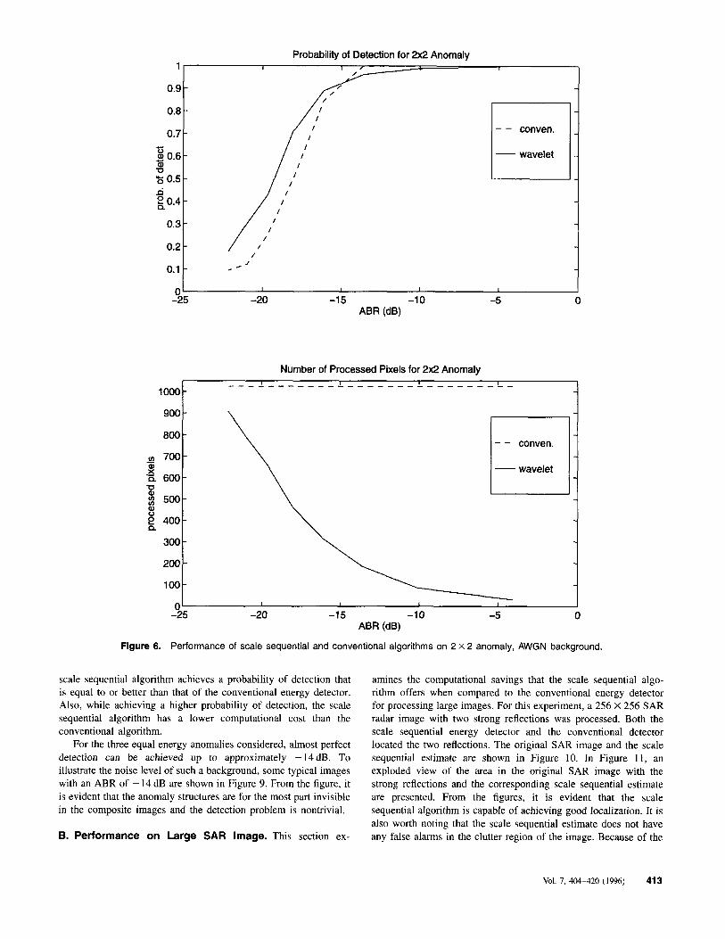
The probability of detection and computational cost of each algorithm has been computed for the anomaly structures of Figure 5. The thresholds used by both algorithms were computed using a constant false alarm rate of Pfo = 0.001. The Haar wavelet basis was used to compute the wavelet transform. The results are presented in Figures 6-8.

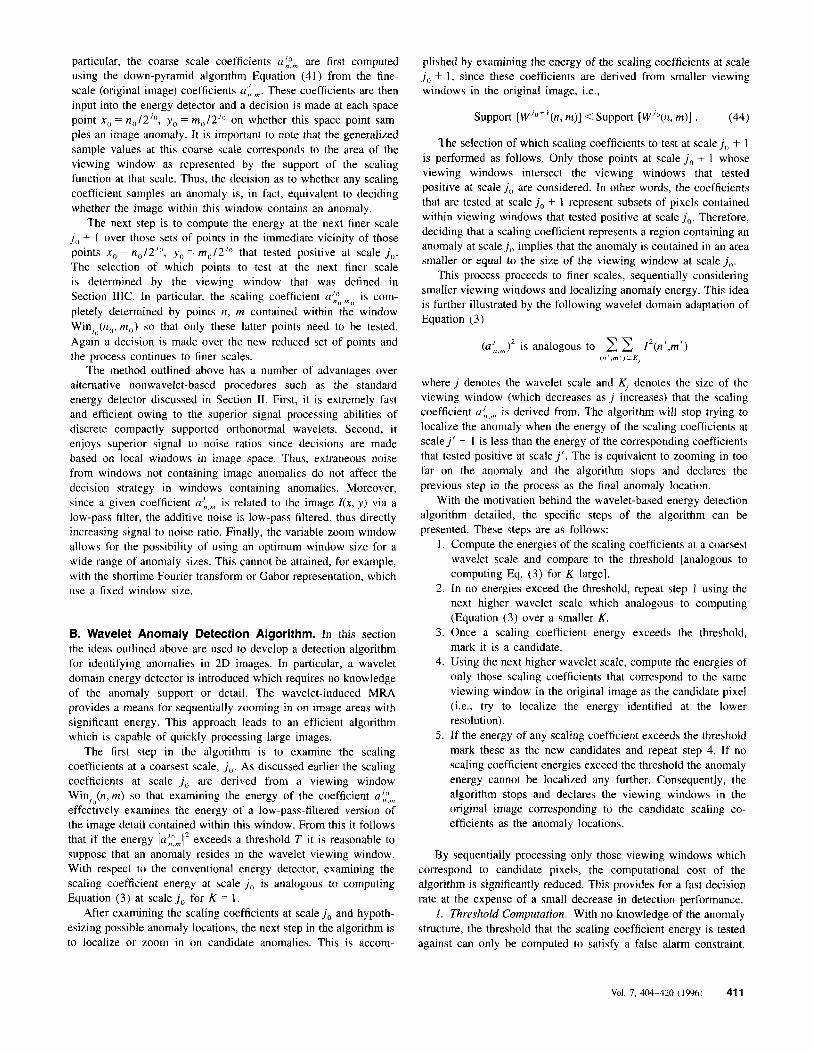
From the graphs, it is evident that the probability of detection for the wavelet-based algorithm is either comparable to or surpas- ses that of the conventional energy detector. The superior per- formance of the scale sequential algorithm was expected, since it was noted in Section I1 that the conventional detector suffers a performance loss for equal energy anomalies with increasing support. The scale sequential algorithm was shown to suffer no such loss. This is evident in the graphs where the performance of the scale sequential algorithm remains approximately constant and the performance of the conventional algorithm decreases with larger anomaly supports. The significance of this result is increased by noting that the conventional detector requires knowledge of the anomaly support, while the scale sequential detector does not. In addition, the scale sequential detector processes far fewer pixels than the conventional detector. This results in significant computa- tional savings with little or no decrease in performance.

In summary, for the anomaly structures that were processed, the

2x2 anomaly structure 4x4 anomaly structure 8x8 anomaly structure

Figure 5. Anomaly structures embedded in synthetic AWGN back- ground.

412 Vol. 7, 404-420 (1996)

Probability of Detection for 2x2 Anomaly

1000

900

800

- v) 700- 2 % 8

E. 600-

$ 500-

9 400-

300

200

100-

0

c

8 0.6 - 5 5 0.5 - n 90.4 - 0.3 -

0.2

0.1

U

-

-

I I I I - - - - - - - _ - - - - _ _ _ - _ _ _ - _ _ _ _ _ _ _ _ _ - - -

-

-

- - - - -

- I I 1 I

/ / r

-

conven.

wavelet

0’ I I I I

-25 -20 -1 5 -1 0 -5 0 ABR (dB)

Figure 6. Performance of scale sequential and conventional algorithms on 2 x 2 anomaly, AWGN background.

scale sequential algorithm achieves a probability of detection that is equal to or better than that of the conventional energy detector. Also, while achieving a higher probability of detection, the scale sequential algorithm has a lower computational cost than the conventional algorithm.

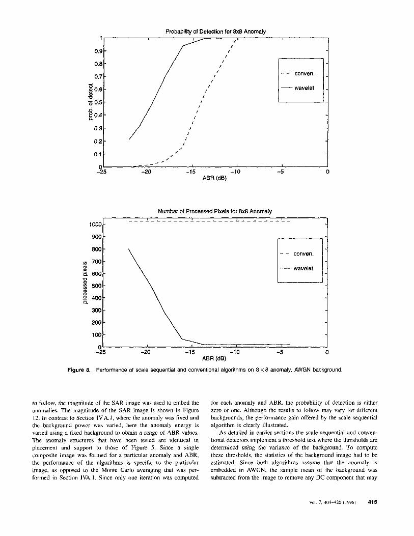
For the three equal energy anomalies considered, almost perfect detection can be achieved up to approximately -14dB. To illustrate the noise level of such a background, some typical images with an ABR of - 14 dB are shown in Figure 9. From the figure, it is evident that the anomaly structures are for the most part invisible in the composite images and the detection problem is nontrivial.

B. Performance on Large SAR Image. This section ex-

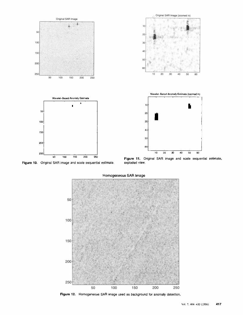
amines the computational savings that the scale sequential algo- rithm offers when compared to the conventional energy detector for processing large images. For this experiment, a 256 X 256 SAR radar image with two strong reflections was processed. Both the scale sequential energy detector and the conventional detector located the two reflections. The original SAR image and the scale sequential estimate are shown in Figure 10. In Figure 1 I , an exploded view of the area in the original SAR image with the strong reflections and the corresponding scale sequential estimate are presented. From the figures, it is evident that the scale sequential algorithm is capable of achieving good localization. It is also worth noting that the scale sequential estimate does not have any false alarms in the clutter region of the image. Because of the

Vol. 7, 404-420 (1996) 413

0.9 - I

I

I

I 1;; I

0.8

0.7

c 0.6

6 0.5 n g0.4

0.3

0.2

c

a, ‘0

conven.

wavelet

-

-

-

-

-

-

-

1

lo00

900

800

- v) 700- 8 .= 600-

500-

g 400-

rn a,

a, 0

300

200

100

0

0‘ I I I I 1 -25 -20 -1 5 -1 0 -5 0

ABR (dB)

I I I I - - - - _ _ _ - - - - - _ _ _ _ - - - - _ _ _ _ _ _ _ _ _ - - -

-

-

-

- - - -

- -

I I I I

strength of the reflections in the SAR image, both algorithms were expected to correctly identify the anomaly. This image was processed to illustrate the computational savings that can be obtained by processing in the wavelet domain. Since the reflections are strong (i.e., they have large amplitude), the wavelet-based

Table I.

algorithm quickly “zooms in” on the reflections and computes far fewer pixel energies than the conventional detector. The number of computed pixel energies is shown in Table I for both algorithms.

From Table I it is evident that for large images with distinct anomalies the scale sequential algorithm is capable of achieving significant computational savings when compared to a conventional energy detector with little or no decrease in performance.

Energy Detection Algorithm No. of Computed Pixel Energies

Scale sequential Conventional

1080 65,536

C. Performance on SAR Clutter. In this section, a homoge- neous SAR image is used as a background for anomalies of varying supports and energy. It should be noted that for the results

414 Vol. 7, 404-420 (1996)

1

0.9

0.8

0.7 c O.."

d 0.4

0.2

I / I

I

/ - / - /

/

/ / conven.

/ / - ,.,3,,nlnt

I - -

0.1 1

I I

I I

I I

I I

I I

/ /

/ a c - - 1 - I I 1 I

-25 -20 -15 -10 -5 0 ABR (dB)

Number of Processed Pixels for 8x8 Anomaly

900

800

y 700 8

$ 500

'5 600 U al

al 0 g 400

300

200

100

J

conven.

wavelet

-

- - -

I I I 1 -20 -15 -10 -5 0

0 -25

ABR (dB)

Figure 8. Performance of scale sequential and conventional algorithms on 8 x 8 anomaly, AWGN background.

to follow, the magnitude of the SAR image was used to embed the anomalies. The magnitude of the SAR image is shown in Figure 12. In contrast to Section IV A. 1 , where the anomaly was fixed and the background power was varied, here the anomaly energy is vaned using a fixed background to obtain a range of ABR values. The anomaly structures that have been tested are identical in placement and support to those of Figure 5. Since a single composite image was formed for a particular anomaly and ABR, the performance of the algorithms is specific to the particular image, as opposed to the Monte Carlo averaging that was per- formed in Section IVA.1. Since only one iteration was computed

for each anomaly and ABR, the probability of detection is either zero or one. Although the results to follow may vary for different backgrounds, the performance gain offered by the scale sequential algorithm is clearly illustrated.

As detailed in earlier sections the scale sequential and conven- tional detectors implement a threshold test where the thresholds are determined using the variance of the background. To compute these thresholds, the statistics of the background image had to be estimated. Since both algorithms assume that the anomaly is embedded in AWGN, the sample mean of the background was subtracted from the image to remove any DC component that may

Vol. 7, 404-420 (1996) 415

2x2 anomaly embedded 2x2 anomaly

Figure 9. Typical images with anomalies embedded in background of ABR= -14dB.

have been present. Next, the sample variance was computed and used with a false alarm constraint of Pf0 = 0.001 to compute the thresholds for each algorithm. The Haar wavelet basis was used to compute the wavelet transform in the scale sequential algorithm.

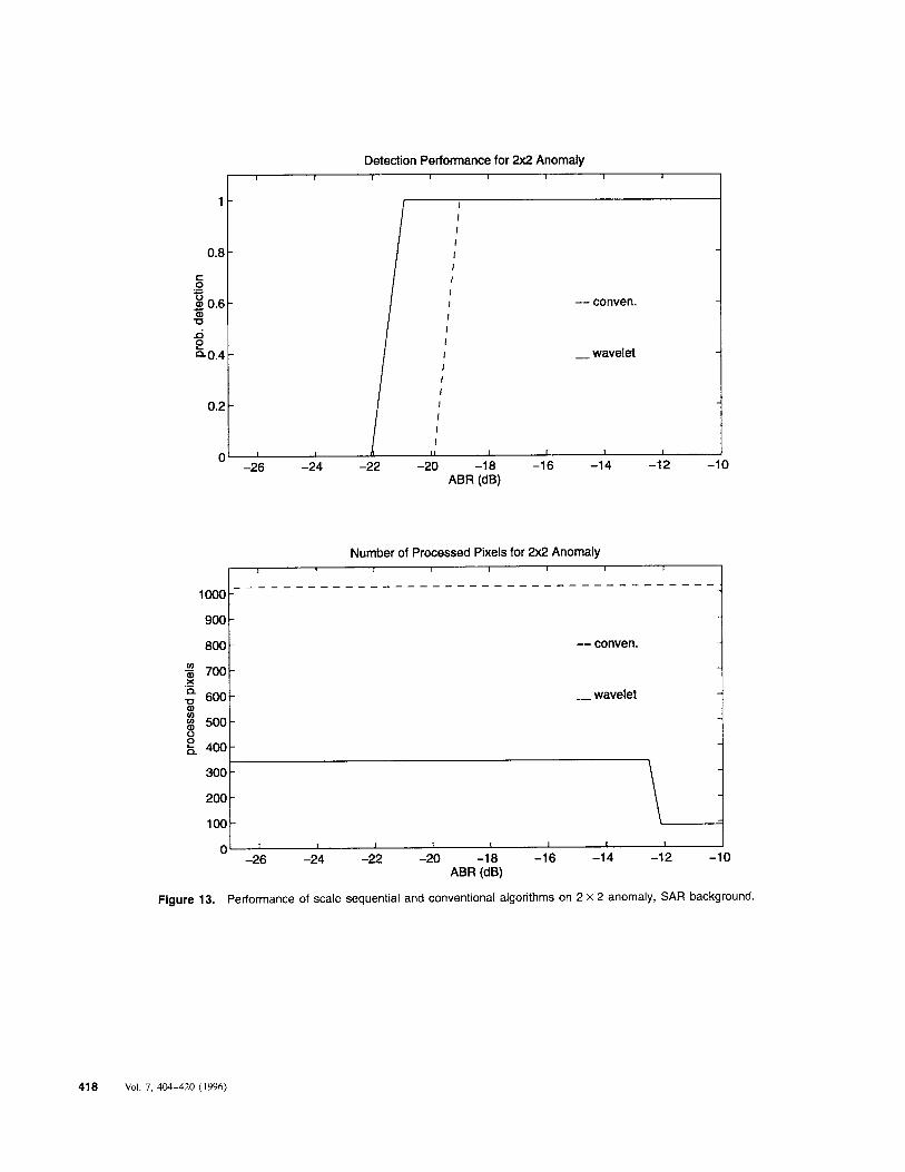
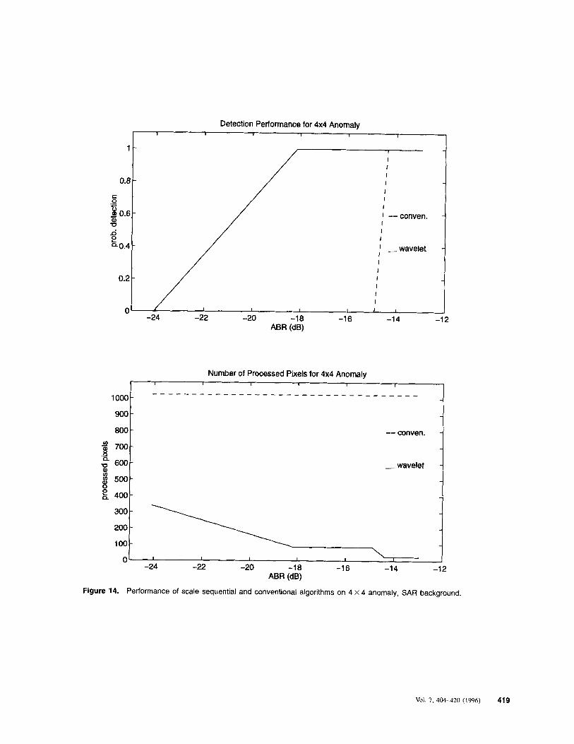
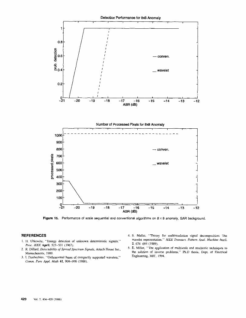
The probability of detection and the computational cost for the three anomaly structures embedded in the SAR background are presented in Figures 13-15 for varying anomaly energy. For each anomaly structure, the scale sequential algorithm correctly detects the anomaly down to a lower ABR than the conventional detector.

In addition the scale sequential detector computes fewer pixel energies than the conventional detector.

In summary, the results show that the scale sequential algorithm achieves a higher level of performance with a lower computational cost for the particular background and anomaly structures consid- ered. This is in agreement with the results of Section IVA.1. In addition, the results show that the scale sequential algorithm works well for the simple estimates used to estimate the background statistics.

416 Vol. 7, 404-420 (1996)

Wavelet-Based Anomaly Estimate

5 0 .

100

150

200

-

-

-

1 I

20: 30

250 50 100 150 200 250

Figure 10. Original SAR image and scale sequential estimate.

I

Wavelet-Based Anomaly Estimate (zoomed in)

I I

1 l o t

Figure 11. Original SAR image and scale sequential estimate, exploded view.

Homogeneous SAR Image

Figure 12. Homogeneous SAR image used as background for anomaly detection.

Vol. 7, 404420 (1996) 417

Detection Performance for 2x2 Anomaly

1OOO-

v) a X a. U a v) v) a 0

- .-

2 a.

-

-- conven.

- wavelet

600

500

400

300

200

100-

0

n I I h I, I I I I

-

-

-

-

- -

- -

- -

I I I I I I I I

-26 -24 -22 -20 -1 8 -1 6 -14 -1 2 -1 0 u

ABR (dB)

Number of Processed Pixels for 2x2 Anomaly

-t 1 700 8001 -- conven.

- wavelet

Figure 13. Performance of scale sequential and conventional algorithms on 2 x 2 anomaly, SAR background.

418 Vol. 7. 404-420 (1996)

1

O.€ c 0 z 3 0.E

d 2 Q0.4

al -0

0.2

0

Detection Performance for 4x4 Anomaly I I I I I I

/

I I I I I I

-24 -22 -20 -18 -1 6 -1 4 -1 2 ABR (dB)

800 gOOl

200 "OI

lWt 0

1 --conven. -1

J

i - wavelet

100 :::: 0 -24 -22 -20 ABR (dB) -18 -1 6 -1 4 -12 -24 -22 -20 -18 -1 6 -1 4 -12

ABR (dB)

Figure 14. Performance of scale sequential and conventional algorithms on 4 x 4 anomaly, SAR background.

Val. 7, 404-420 (1996) 419

1 1 I L I I I 1

1 - I - I

I I

0.8 - I I

K I I 0

I - .- -

-- conven. I

I

0.6 - c a U

n I e I - wavelet I I

I I

I I

I

Q0.4 -

- 0.2 -

0 I I I 1 I I

Number of Processed Pixels for 8x8 Anomaly I 1 I I I I I I

800 gml -- conven.

-wavelet

=: 100 0

-21 -20 -19 -18 -17 -16 -15 -14 -13 -12 ABR (dB)

Figure 15. Performance of scale sequential and conventional algorithms on 8 x 8 anomaly, SAR background.

REFERENCES 4. S. Mallat, “Theory for multiresolution signal decomposition: The wavelet representation,” IEEE Transact. Pattern Anal. Machine Intell. 1. H. Urkowitz, “Energy detection of unknown deterministic signals,” 2, 674-693 (1989).

2. R. Derecrabirjo ofspread 5. E. Miller, “The application of multiscale and stochastic techniques to the solution of inverse problems,” Ph.D thesis, Dept. of Electrical

3. I. Daubechies, “Orthonormal bases of compactly supported wavelets,” Engineering, MIT, 1994.

Proc. IEEE April, 523-531 (1967).

Massachusetts, 1989.

Comrn. Pure Appl. Math 41, 909-996 (1988).

House

420 Vol. 7, 404-420 (1996)