Wavelet-based methods to analyse, compress and...

Wavelet-based methods to analyse, compress and compute

turbulent flows

Marie Farge Laboratoire de Météorologie Dynamique

Ecole Normale Supérieure Paris

Mathematics of Planet Earth Imperial College, London

4th November 2015

Outline

1. Choice of an adequate representation

2. The wavelet transform and its multiscale representation

Continuous wavelet transform Orthogonal wavelet transform

Wavelet-based filtering and denoising

3. Applications to 2D and 3D turbulent flows

What is turbulence? Extraction of coherent structures

New interpretation of the turbulent cascade Wavelet-based numerical simulation

'A representation is a formal system for making explicit certain entities or types of information, together with a specification of how the system does this. For example, the Arabic, Roman and binary numerical systems are formal systems for representing numbers. […] A representation therefore is not a foreign idea at all, we all use representations all the time. However, the notion that we can capture some aspects of reality by making a description of it using a symbol, and that to do so can be useful, seems to me a fascinating and powerful idea ... This issue is important, because how information is presented can greatly affect how easy it is to do different things with it. This is evident even from our number example : it is easy to add, to subtract and even to multiply if the Arabic or binary representation are used, but it is not at all easy to do these things, especially multiplication, with Roman numerals. This is a key reason why the Roman culture failed to develop mathematics in the way the Arabic culture had.’

Choice of an adequate representation

David Marr !Vision !Freeman,1982!

An adequate representation for music

Guido d’Arezzo Micrologos

1025

ut re mi fa sol la si sa re ga ma pa da ni

7 tones:

12 half tones:

Discrete grid-point

representation :

Discrete Fourier

representation :

Phase-space (x,k)

Integral transforms

A A

Analysis :

Synthesis :

Uncertainty principle :

Continuous Fourier transform (1807)

Analysis

Synthesis

Plancherel’s identity

Function to analyze :

Fourier coefficients :

Reconstructed function :

€

⇒ Energy conservation

Fourier modes as analyzing

functions:

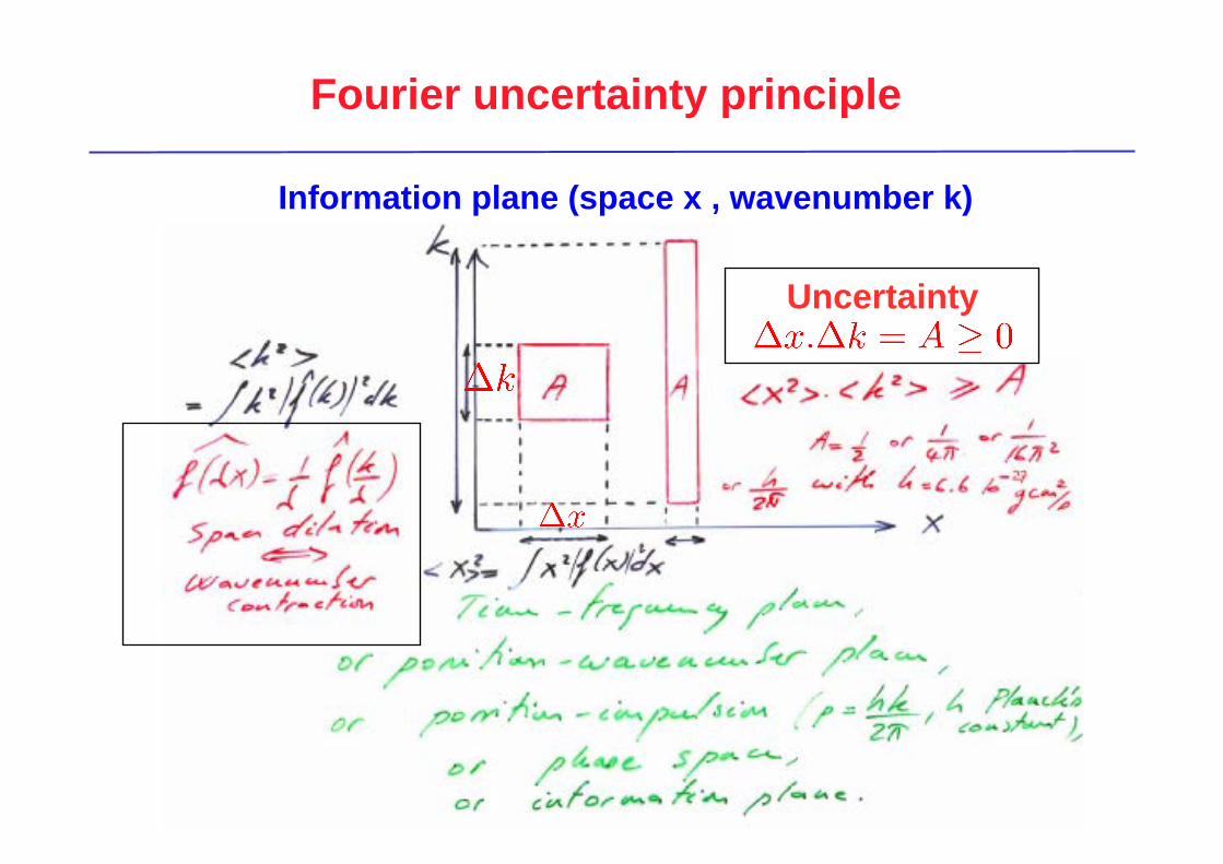
Uncertainty

Information plane (space x , wavenumber k)

Fourier uncertainty principle

Windowed Fourier

representation (1946) :

Wavelet representation

(1984) :

Optimal tiling of phase-space

Space-wavenumber representation

Space-scale representation information atom

The Wavelet Transform and its Multiscale Representation

The ‘mother’ wavelet should verify an

admissibility condition :

By translating and dilating it, one generates a

family of analyzing wavelets : Alex Grossmann Jean Morlet

Grossmann and Morlet, Decomposition of Hardy functions into square

integrable wavelets of constant shape, SIAM J. math. Anal., 15(4), 723-736, 1984

Choice of a ‘mother’ wavelet

Generation of the family of wavelets

In physical space : In spectral space :

€

ψ ji

€

ˆ ψ ji

€

j = 3

€

j = 4

€

j = 5

€

j = 6

€

j = 7

€

iΔk

Δx

Farge, Wavelet transforms and

their applications to turbulence Ann. Rev. Fluid Mech., 92, 1992

Farge and Schneider, Wavelets: application to turbulence,

Encyclopedia of Mathematical Physics, Springer, 408-42, 2006

Continuous wavelet transform (1984)

Analysis

Synthesis

Plancherel’s identity

Wavelet coefficients :

Reconstructed function :

€

⇒ Energy conservation

Wavelet modes :

Haar measure :

if

2D continuous wavelet transform

2D Morlet ‘mother’ wavelet

The wavelet family is generated by translating, dilating and rotating

2D mother wavelet

Modulus of the wavelet

coefficients

Analyzing wavelet

Field to analyze

Small scale

Large scale

Logarithm of the scale

2D real-valued Marr wavelet

Bandpass filter with Δk/k constant

2D complex-valued Morlet wavelet

The CWT acts as a local filter in k-space and as a polarizor

Discrete multiscale wavelet representation

We can then select a finite number of wavelets restricted to a discrete grid optimally chosen, such that

the wavelet family associated to this grid constitutes a quasi-orthogonal basis a wavelet frame

€

⇒

For example for Marr wavelet

we need : a0=21/2

b0=1/2

Orthogonal wavelet transform

Wavelet analysis :

Wavelet synthesis :

A signal sampled on N points is wavelet analyzed and synthetized in CN operations

if one uses compactly-supported wavelets computed from a quadrature mirror filter of length C.

with

Orthogonal wavelet representation

Wavelet coefficients

scale j

position i

€

ψ ji

N = 512 = 29

Mallat, 1998 A wavelet tour of

signal processing, 3rd edition, Academic Press

Wavelets

~ f f jiji ψ=

The dyadic grid of the orthogonal wavelet space

2D orthogonal wavelets

Coarse approximation

Vertical details

Horizontal details

Diagonal details

‘The father’: scaling function low-pass filter

‘The mother’: wavelet,

band-pass filter

Image sampled on N=5122=(29)2 pixels N=5122 wavelet coefficients

2D orthogonal wavelet representation

Wavelet-based Filtering and Denoising

162=0.1% N wavelet coefficients Image reconstructed up to scale 24

Linear compression


Linear compression

2562=25% N wavelet coefficients Image reconstructed up to scale 28

Linear compression

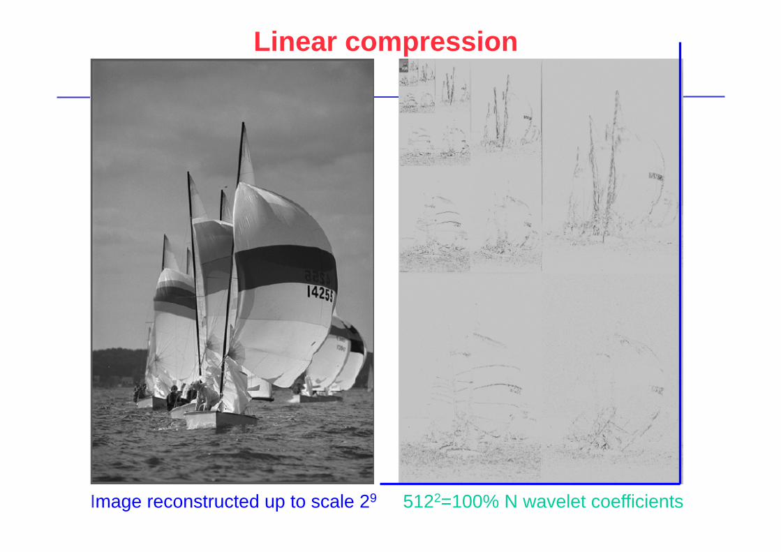
5122=100% N wavelet coefficients Image reconstructed up to scale 29

Linear compression

Local linear compression

Image locally reconstructed up to scale 25


Image reconstructed up to scale 26


Image loccaly reconstructed up to scale 29

Image sampled on N=(29)2 pixels N=5122 wavelet coefficients

Nonlinear compression

3.3% N wavelet coefficients Image reconstructed from 3.3% N


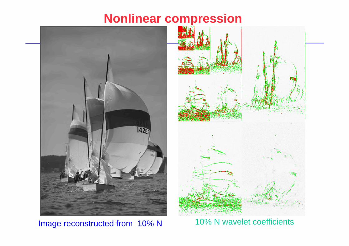
10% N wavelet coefficients Image reconstructed from 10% N


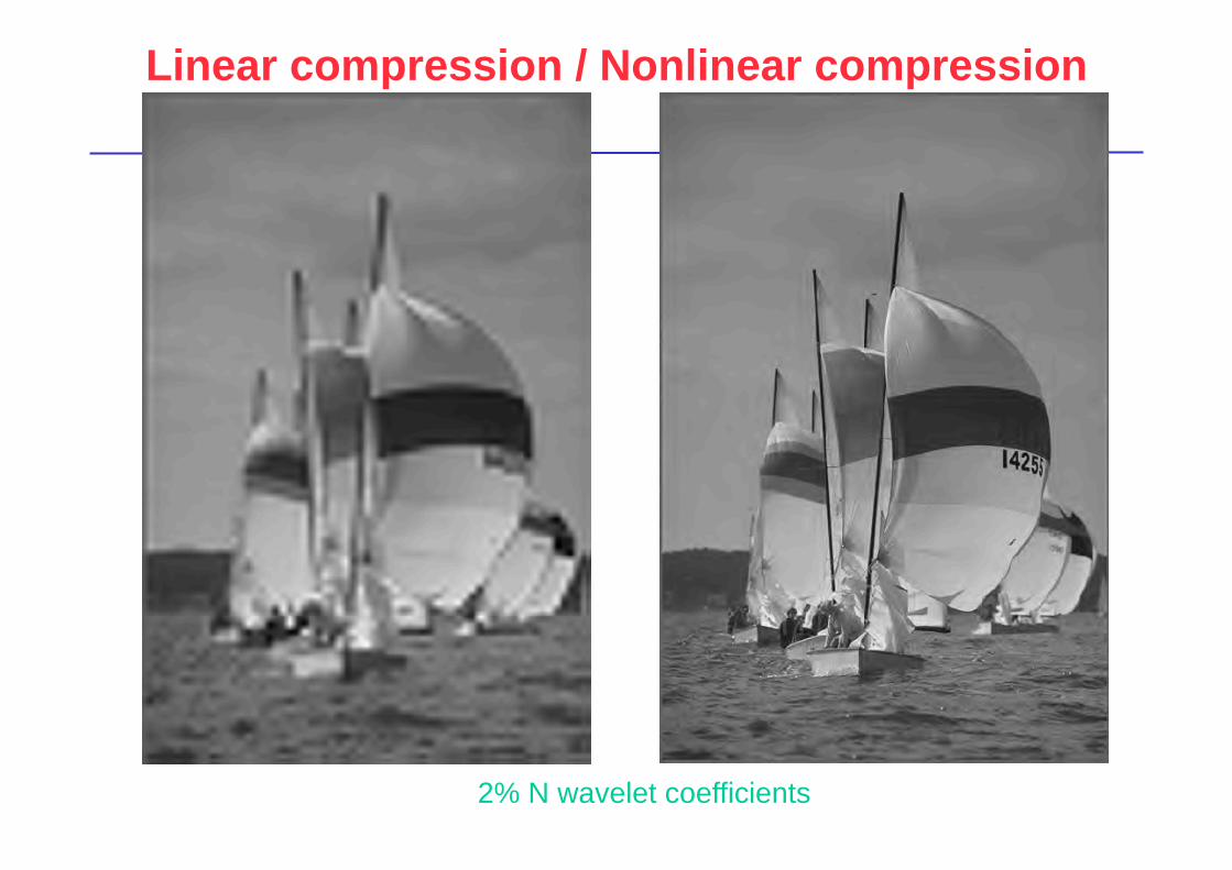
2% N wavelet coefficients

Linear compression / Nonlinear compression

Wavelet-based denoising

Gaussian white noise is by definition equidistributed among all modes and the amplitude of the coefficients is given by its r.m.s.

whatever the functional basis one considers to represent it.

Therefore the coefficients of a noisy signal whose amplitudes are larger than the r.m.s. of the noise belong to the denoised signal.

This procedure corresponds to wavelet-based denoising.

The advantage of such a nonlinear filtering using the wavelet representation is that the wavelet coefficients preserve the space-scale locality, since

wavelets are functions localized in both physical and spectral space.

Since we do not know a priori the r.m.s. of the noise, we have proposed an iterative procedure which takes as first guess the r.m.s. of the noisy signal.

Azzalini, M. F., Schneider, 2005 Appl. Comput. Harmonic Analysis, 18 (2)

Donoho, Johnstone, Biometrika, 81, 1994

Apophatic method : - no hypothesis on the structures, - only hypothesis on the noise, - simplest hypothesis as our first choice.

Hypothesis on the noise : fn = fd + n

n Gaussian white noise, <fn2> variance of the noisy signal, N number of coefficients of fn.

Wavelet decomposition :

Estimation of the threshold :

Wavelet reconstruction :

€

εn = 2 < fn2 > ln(N)

€

fd = f~

jiψ ji

ji: f~

ji >ε n

∑

f

€

fn

€

fd

Wavelet-based denoising algorithm

€

˜ f ji =< f |ψ ji >j scale, i position

Azzalini, M. F., Schneider, ACHA, 18 (2), 2005

Donoho, Johnstone, Biometrika, 81, 1994

Application to turbulent flows

Turbulence is a state that fluid, gas or plasma flows reach when they become unstable and highly fluctuating.

Etymology of the word ‘turbulence’ : turba-ae, crowd, mob

turbo-inis, vortex A mob of vortices interacting together on a wide range of temporal and spatial scales.

What is turbulence?

The turbulent regime corresponds to the limit where the nonlinear terms dominate the linear terms.

The flow is then highly unstable, chaotic and mixing.

Incompressible flows are governed by 3D Navier-Stokes equations

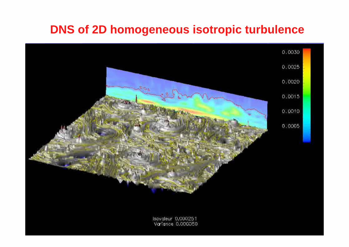
DNS of 2D homogeneous turbulence

DNS N=5122

Negative vorticity

Positive vorticity

No vorticity

Farge, 1987, Advances

In turbulence

DNS of 2D homogeneous isotropic turbulence DNS

N=5122

Extraction of coherent structures

Since there is not yet a universal definition of coherent structures which emerge out of turbulent fluctuations due to the nonlinear interactions,

we adopt an apophatic method : instead of defining what they are, we define what they are not.

Choosing the simplest hypothesis as a first guess, i.e., Occam’s razor principle, we suppose we want to eliminate an additive Gaussian white noise,

and for this we use a nonlinear wavelet-based filtering. €

⇒

Farge, Schneider et al., Phys. Fluids, 15 (10), 2003

Extracting coherent structures becomes a denoising problem, not requiring any hypotheses on the structures themselves

but only on the noise to be eliminated.

For this we propose the minimal statement : ‘Coherent structures are not noise’

Azzalini, Farge, Schneider, ACHA, 18 (2), 2005

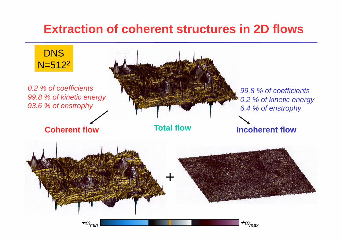
Total flow

0.2 % of coefficients 99.8 % of kinetic energy 93.6 % of enstrophy


Incoherent flow Coherent flow

+ωmin +ωmax

+

DNS N=5122

Extraction of coherent structures in 2D flows

1D cut of the vorticity field

DNS N=5122

ωt=ωc+ωi

Zt=Zc+Zi

Total

Coherent 0.2 % N 99.8 % E 93.6 % Z

Incoherent 99.8 % N 0.2 % E 6.4 % Z

ωmin

log p(ω)

PDF of vorticity

DNS N=5122

Total

Coherent 0.2 % N 99.8 % E 93.6 % Z

ωmax

Incoherent 99.8 % N 0.2 % E 6.4 % Z

Enstrophy spectrum

Coherent

k-5 scaling, i.e. long-range

correlation

log k

log Z(k)

Incoherent

k-1 scaling, i.e. enstrophy equipartition since E=k-2 Z

DNS N=5122

Coherent 0.2 % N 99.8 % E 93.6 % Z

Incoherent 99.8 % N 0.2 % E 6.4 % Z

Total

A posteriori proof of coherence

Coherent Incoherent

DNS N=5122

Total

Coherent structures are locally (in space and time)

steady solutions of Euler equation, thus, for 2D flows :

Arnold, 1965, Joyce & Montgomery, 1973 Robert & Sommeria, 1991

ω = sinh(ψ)

ψ ψ

ω ω ω

DNS of 2D homogeneous isotropic turbulence

• Rotate up to 1.0 Hz • Mechanical pumping of fluid

through hexagonal array of sources and sinks

• 100 mm seed particles

• PIV to measure velocity fields and calculate vorticity fields

2D turbulent flow observed in a rotating tank

Coherent vorticity 99% E 80% Z

Incoherent vorticity 1% E 3% Z

Total vorticity 100% E 100% Z

2% N 98% N

-ωmin -ωmax

PIV N=1282

Extraction of coherent structures in 2D flows

Coherent vorticity 99% E 80% Z

Incoherent vorticity 1% E 3% Z

Total vorticity 100% E 100% Z

2% N 98% N

-ωmin -ωmax

DNS N=1282

Passive scalar advection

by the total flow by the coherent flow by the incoherent flow

Advection of tracer particles

Diffusion by Brownian motion

Transport by vortices

= +



Beta, Schneider, Farge 2003, Nonlinear Sci. Num. Simul., 8

DNS N=1282

3D fully-developed homogeneous turbulent flow

Kaneda et al., 2003 Phys. Fluids, 12, 21-24

Rλ

20483 40963

1200

10243 5123

Fully-developed turbulence

Dissipation rate α

Transition

When the fully-developed turbulent regime is reached the dissipation rate becomes independent of the Reynolds number

L

２π

Modulus of the vorticity field (20483)

L, integral scale

Resolution N=20483

Kaneda, et al., 2003,

Phys. Fluids, 12, 21-24

Computed in 2002 on ES1

14 Tflops 10 Tbytes

L

λ

Zoom (sub-cube 10243 )

Resolution N=20483

λ, Taylor micro- scale

L, Integral scale

Kaneda et al., 2003,


L

λ

Resolution N=20483

L, integral scale λ, Taylor macro- scale


Kaneda et al., 2003, Phys. Fluids,

12, 21-24

λ η

η, Kolmogorov dissipative scale

Resolution N=20483

λ, Taylor macro- scale




DNS N=20483




DNS N=20483


Kaneda, et al., 2003,


Total vorticity

+

2.6 % N coefficients 80% enstrophy

99% energy

97.4 % N coefficients 20 % enstrophy

1% energy

Incoherent vorticity Coherent vorticity

DNS N=20483

Extraction of coherent structures

|ω|=5σ

|ω|=5σ

|ω|=5/3σ

with σ=(2Ζ)1/2

Okamoto, Yoshimatsu, Schneider, Farge,

Kaneda, 2007, Phys. Fluids, 19, 1159

Multiscale Coherent k-5/3 scaling, i.e.

long-range correlation

Multiscale Incoherent k+2 scaling, i.e.

energy equipartition

DNS N=20483

Energy spectrum

k-5/3

2.6 % N coefficients 80% enstrophy

99% energy

k+2 log E(k)

Okamoto , Yoshimatsu, Farge, Schneider,

Kaneda, 2007 Phys. Fluids, 19(11)

log k

DNS N=20483

PDF of velocity

The total and coherent flows have the same extrema. The incoherent flow has a Gaussian PDF,

therefore its effect should be easy to model

log p(v)

2.6 % N coefficients 99% energy

Okamoto , Yoshimatsu, Farge, Schneider,

Kaneda, 2007 Phys. Fluids, 19(11)

v

Nonlinear transfers and energy fluxes

ttt cci

icc, iic

ccc coherent flux

= total flux

iic, iii incoherent flux = 0

Inertial range

L η

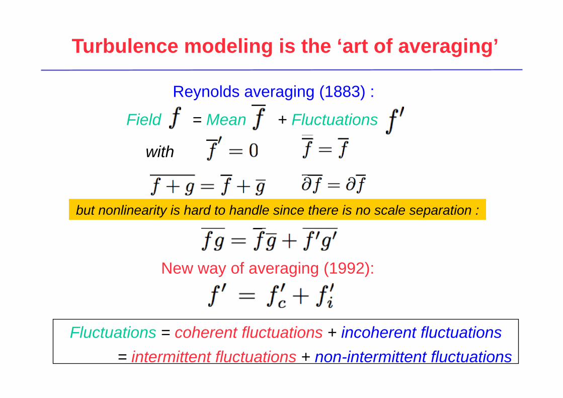
Turbulence modeling is the ‘art of averaging’

Reynolds averaging (1883) :

New way of averaging (1992):

with

Fluctuations = coherent fluctuations + incoherent fluctuations = intermittent fluctuations + non-intermittent fluctuations

but nonlinearity is hard to handle since there is no scale separation :

Field = Mean + Fluctuations

Decomposition of turbulent flows ‘In 1938 Tollmien and Prandtl suggested that turbulent fluctuations might consist of two components, a diffusive and a non-diffusive. Their ideas that fluctuations include both random and non random elements are correct, but as yet there is no known procedure for separating them.’

Hugh Dryden, Adv. Appl. Mech., 1, 1948

mean + turbulent fluctuations = mean + non random + random

= mean + coherent structures + incoherent noise

Farge, Schneider, Kevlahan, Phys. Fluids, 11 (8), 1999

Farge, Ann. Rev. Fluid Mech., 24,1992

Farge, Pellegrino, Schneider Phys. Rev. Lett., 87 (5), 2001

€

⇒ Coherent Vorticity Simulation (CVS)

turbulent dynamics = chaotic non diffusive + stochastic diffusive

= inviscid nonlinear dynamics + turbulent dissipation €

⇒ Coherent Vorticity Extraction (CVE)

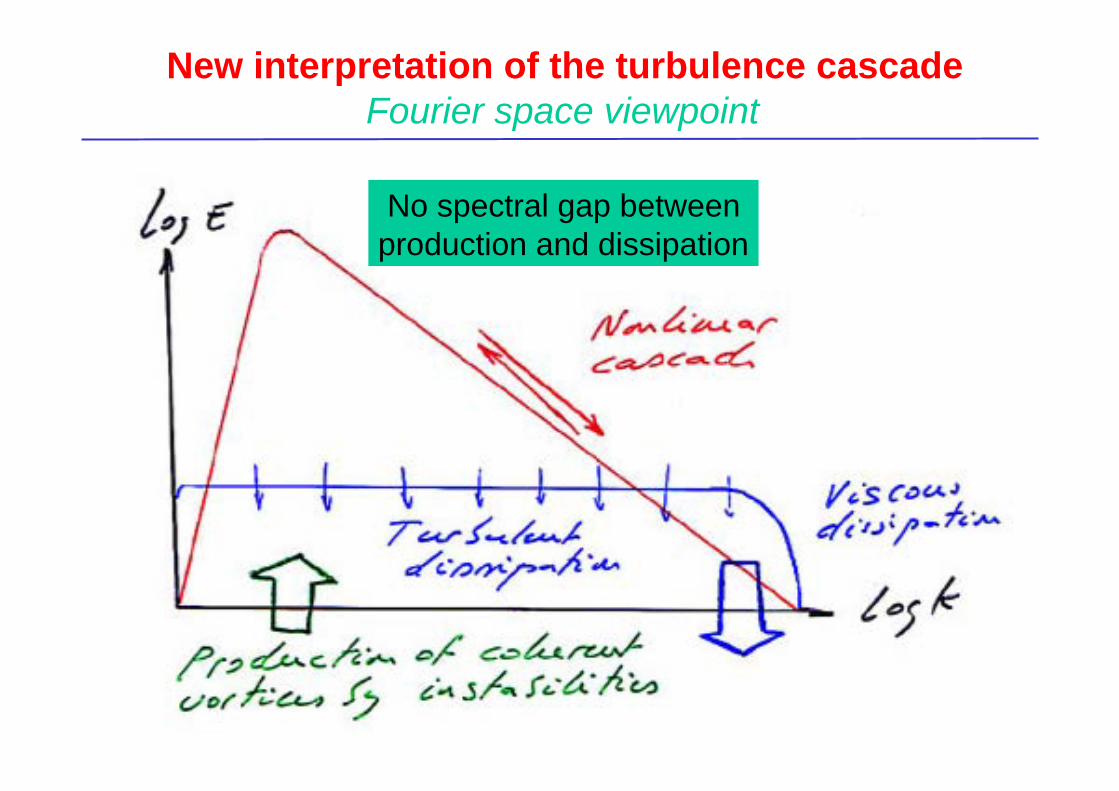
New interpretation of the turbulence cascade Fourier space viewpoint

No spectral gap between production and dissipation

New interpretation of the turbulence cascade Physical space viewpoint

Vortex stretching and bursting

No vortex fission ‘a la Richardson’

Linear dissipation

Nonlinear interactions

Interface η

Small scales

Large scales

<η>

New interpretation of turbulence cascade Wavelet space viewpoint

Wavelet-based Numerical Simulation

1. Selection of the wavelet coefficients whose modulus

is larger than the threshold.

2. Construction of a ‘graded-tree’ which defines the ‘interface’ between the coherent and incoherent wavelet coefficients.

3. Addition of a ‘security zone’ which corresponds to dealiasing.

Coherent Vorticity Simulation (CVS)

Schneider & Farge, 2002, Appl. Comput. Harmonic Anal., 12

Schneider, Farge et al., 2005, J. Fluid Mech., 534(5)

Schneider & Farge, 2000, Comp. Rend. Acad. Sci. Paris, 328

Vorticity dipole impinging on a wall

Adapted grid automatically generated by CVS

CVS of Kelvin-Helmholtz instability in 2D

Schneider, Farge, Koster,Griebel , Numerical Flow Simulation, 75,

Springer, 303-318, 2001

DNS CVS

Comparison DNS / CVS for 3D mixing layer

4 eddy turnover times

Schneider, Farge, Pellegrino, Rogers 2005,

J. Fluid Mech., 534(5)

DNS CVS





MPE Wednesday - Programme for Term 1

Academic Year 2014/2015

Date

Location Speaker Title

8th October 2014

Imperial

College London

Prof Hans Kaper

Georgetown University

Mathematics and

Climate: A New

Partnership

29th October 2014

University of

Reading

Prof Jacques Vanneste

University of Edinburgh

Interactions between

near-inertial waves and

mesoscale motion in the

ocean

5th November 2014

Imperial

College London

Robert Scheichl

University of Bath

Novel Multilevel Monte

Carlo Methods for the

Earth Sciences

12th November 2014

University of

Reading

Roland Potthast

German Weather Service (DWD)

and University of Reading

Modern Data Assimilation

for Numerical Weather

Prediction

19th November 2014

Imperial

College London

Rupert Klein

Freie Universität Berlin

Multi-scale asymptotic

analyses of atmospheric

motions

26th November 2014

University of

Reading

John Thuburn

University of Exeter

Geometry and

atmospheric modelling

3rd December 2014

University of

Reading

Alex Mahalov

Arizona State University

Decadal and Regional

Climate Prediction using

Earth System Models:

Seeking Sustainable

Solutions for Rapidly

Expanding Urban Areas

10th December 2014

Imperial

College London

Peter Ashwin

University of Exeter

Bifurcation, noise and

rate dependent tipping in

open systems

17th December 2014

Imperial

College London

Chris Budd

University of Bath

TBC

Source: CEA

Present General Simulation Models

Clouds

Oceans

Topography

Vegetation

Computational grid

Adaptative icosahedric grid generated using

bi-orthogonal wavelets

Thomas Dubos (LMD, France)

et Nicholas Kevlahan (McMasters, Canada)

Future General Simulation Models

‘As long as we are not able to predict the drag on a sphere or the pressure drop in a pipe from continuous, incompressible and Newtonian assumptions without any other complications, namely from first principles, we would not have made it!’

Turbulence Workshop, UC Santa Barbara,

1997

Hans Liepmann (1914-2009)

Turbulence is still an open problem!

Turbulence is still an open problem for physicists and mathematicians. Indeed,

the Berlin 1750 Prize problem posed by Euler is not yet solved!

Review papers on wavelets

Marie Farge, 1992 Wavelet Transforms and Their Applications to Turbulence Ann. Rev. Fluid Mech., 24, 395-457

Marie Farge, Nicholas Kevlahan, Valerie Perrier and Eric Goirand, 1996 Wavelets and Turbulence IEEE Proceedings, 84, 4, 1996, 639-669

Marie Farge, Nicholas Kevlahan, Valérie Perrier and Kai Schneider, 1999 Turbulence Analysis, Modelling and Computing using Wavelets Wavelets in Physics, ed. J. van den Berg, Cambridge University Press, 117-200

Marie Farge and Kai Schneider, 2002 Analyzing and computing turbulent flows using wavelets

Summer Course, Les Houches LXXIV, New trends in turbulence, Springer

Kai Schneider and Marie Farge, 2006 Wavelets: Mathematical Theory Encyclopedia of Mathematical Physics, Elsevier, 426-437

Marie Farge and Kai Schneider, 2015 Wavelets transforms and their applications to MHD and plasma turbulence Journal of Plasma Physics, Cambridge University Press, in press

You can download movies from :

‘Results’

You can download papers from : ‘Publications’

You can download codes from :

‘Codes’

http://wavelets.ens.fr

Wavelet-based methods to analyse, compress and...

Documents

Transcript of Wavelet-based methods to analyse, compress and...