
Waveform Diversity and MIMO Radarrsadve/Notes/WaveformDiversityMIMO... · – a generalization of...
109
Waveform Diversity and MIMO Radar Raviraj S. Adve Edward S. Rogers Sr. Dept. of Elec. and Comp. Eng. University of Toronto 10 King’s College Road d Toronto, ON, Canada M5S 3G4 Tel: (416) 946 7350 E-mail: rsadve@comm utoronto ca E mail: rsadve@comm.utoronto.ca IRSI’11 December 2011
Transcript of Waveform Diversity and MIMO Radarrsadve/Notes/WaveformDiversityMIMO... · – a generalization of...
Waveform Diversity and MIMO Radar
Raviraj S. AdveEdward S. Rogers Sr. Dept. of Elec. and Comp. Eng.
University of Toronto10 King’s College Road
dToronto, ON, Canada M5S 3G4
Tel: (416) 946 7350E-mail: rsadve@comm utoronto caE mail: [email protected]
IRSI’11 December 2011
Overview
• Radar basics and backgroundwaveforms– waveforms
•pulse compression
•ambiguity function•ambiguity function
– phased array radars
– STAPSTAP
– target models
– early look at waveform diversityearly look at waveform diversity
IRSI’11 December 2011
Overview (2)
• MIMO Radar– importance of diversity– importance of diversity
– virtual array representation
– theoretical analysestheoretical analyses•target models
•diversity ordery
– STAP with distributed sensors
• MIMO and Waveform Diversityy– MIMO ambiguity function
– waveform design
IRSI’11 December 2011
– fast-time & slow-time MIMO
I : Radar Basics
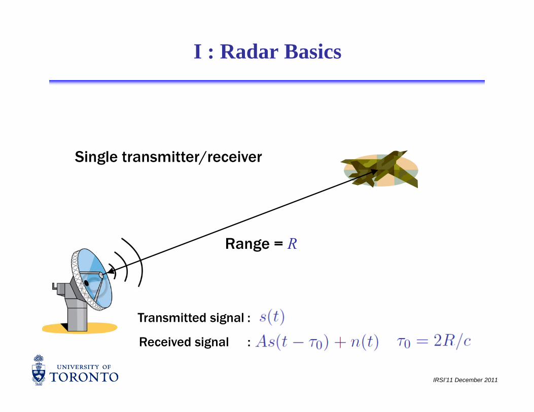
Single transmitter/receiver
Range = R
Transmitted signal :
IRSI’11 December 2011
Received signal :
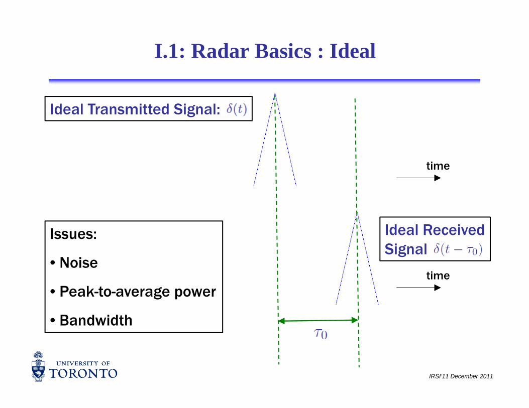
I.1: Radar Basics : Ideal
Ideal Transmitted Signal:
time
Ideal Received I Ideal Received Signal
time
Issues:
• Noise
• Peak-to-average power
• Bandwidth
IRSI’11 December 2011
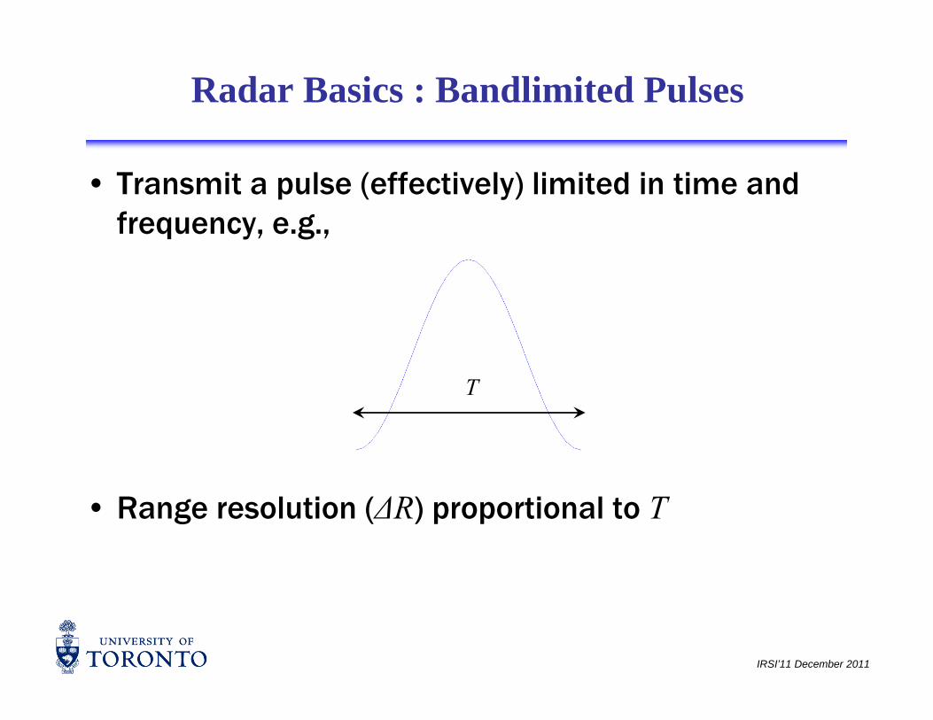
Radar Basics : Bandlimited Pulses
• Transmit a pulse (effectively) limited in time and frequency e gfrequency, e.g.,
T
∆• Range resolution (∆R) proportional to T
IRSI’11 December 2011
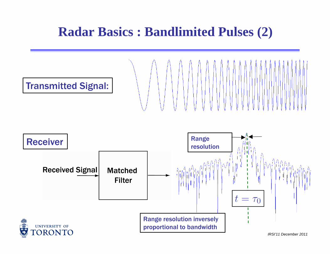
Radar Basics : Bandlimited Pulses (2)
Transmitted Signal:
Receiver Range Receiver resolution
IRSI’11 December 2011
Range resolution inversely proportional to bandwidth
Radar Basics : Bandlimited Pulses (3)
• Matched filter: ;: gathers all energy in
D t t t g t b fi di g th i f th t t • Detect target by finding the maximum of the output of the matched filter
target declared present if signal above some threshold– target declared present if signal above some threshold
– target range from round-trip time
• This is equivalent to pulse compression• This is equivalent to pulse compression– transmitted signal spread over long time
– receiver creates very narrow signal in time– receiver creates very narrow signal in time•range resolution inversely proportional to bandwidth
(∆R ≈ c/2B)
IRSI’11 December 2011
•improvement in resolution ≈ time-bandwidth product
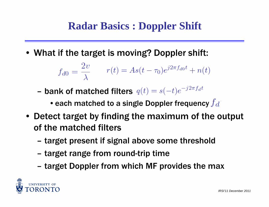
Radar Basics : Doppler Shift
• What if the target is moving? Doppler shift:
bank of matched filters– bank of matched filters•each matched to a single Doppler frequency
• Detect target by finding the maximum of the output • Detect target by finding the maximum of the output of the matched filters– target present if signal above some thresholdtarget present if signal above some threshold
– target range from round-trip time
– target Doppler from which MF provides the max
IRSI’11 December 2011
ta get opp e o c p o des t e a

Radar Basics : Ambiguity Function
• Range-Doppler resolution determined by the ambiguity functionambiguity function
IRSI’11 December 2011
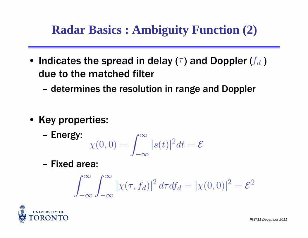
Radar Basics : Ambiguity Function (2)
• Indicates the spread in delay ( ) and Doppler ( ) due to the matched filterdue to the matched filter– determines the resolution in range and Doppler
• Key properties:Energy: – Energy:
– Fixed area: – Fixed area:
IRSI’11 December 2011
Background : Popular Waveforms
• Linear FM: FM modulate a linear signalinstantaneous frequency is proportional to time– instantaneous frequency is proportional to time
– time shift implies a frequency shift…• leading to a coupling in range and Doppler•…leading to a coupling in range and Doppler
– constant envelope signal
– Doppler tolerant in that characteristics e g Doppler tolerant in that characteristics, e.g., sidelobes, not affected by Doppler shift of target
• Phase-coded waveforms– Subdivide a long pulse into “chips”
– in each chip use a different phase for the transmit
IRSI’11 December 2011
p pwaveform

Background : Popular Waveforms (2)
• Resolution function of chip length, not pulse length
C h th h t g i i i • Can choose the phase sequence to e.g., minimize sidelobe levels
• Biphase codes• Biphase codes– phases of 0 and 180 degrees only
Barker codes– Barker codes•achieve best peak-to-sidelobe ratio
– Maximal length sequencesMaximal length sequences•low peak sidelobes, high average sidelobes compared
to LFM
IRSI’11 December 2011
•poor spectral characteristics without bandlimiting
Background : Popular Waveforms (3)
• Polyphase codespolyphase Barker codes through exhaustive search– polyphase Barker codes through exhaustive search
– Frank, P1 and P2 codes•lower sidelobe levels for same length•lower sidelobe levels for same length
•P1 and P2 codes are robust to bandlimiting
•All have poor Doppler tolerancea e poo opp e to e a ce– range sidelobes raise dramatically with Doppler
•P3 and P4 codes mimic LFM and can be robust to b dli iti (P4)bandlimiting (P4)
IRSI’11 December 2011
I.2 : Phased Arrays
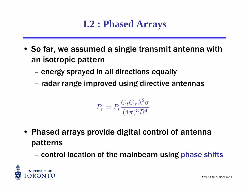
• So far, we assumed a single transmit antenna with an isotropic patternan isotropic pattern– energy sprayed in all directions equally
– radar range improved using directive antennas– radar range improved using directive antennas
• Phased arrays provide digital control of antenna • Phased arrays provide digital control of antenna patterns– control location of the mainbeam using phase shifts
IRSI’11 December 2011
control location of the mainbeam using phase shifts
Phased Arrays (2)
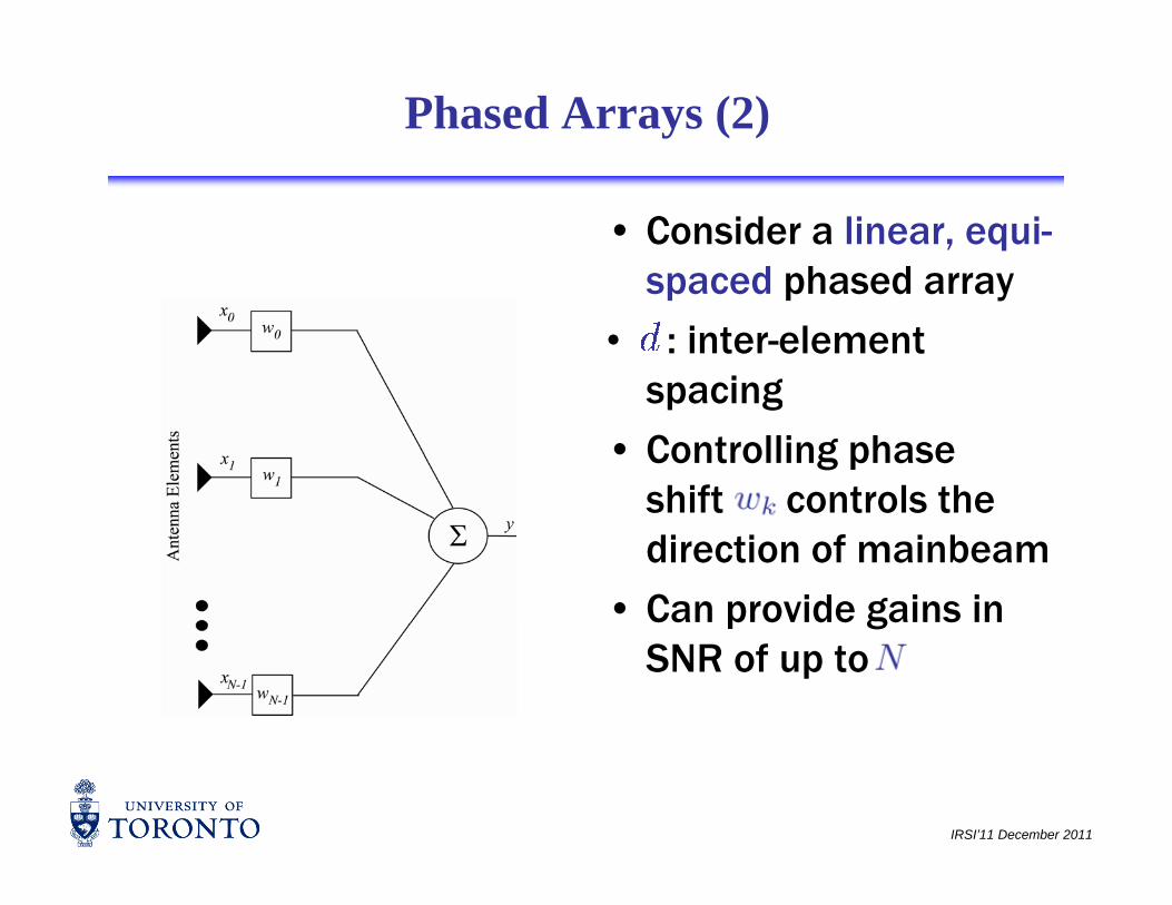
• Consider a linear, equi-spaced phased arrayspaced phased array
• : inter-element spacingspacing
• Controlling phase shift controls the shift controls the direction of mainbeam
• Can provide gains in p gSNR of up to
IRSI’11 December 2011
Phased Arrays (3)
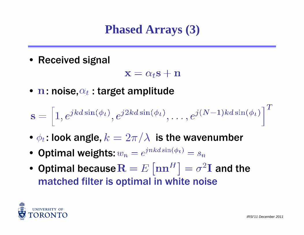
• Received signal
• : noise, : target amplitude
• : look angle, is the wavenumber
• Optimal weights:
• Optimal because and the matched filter is optimal in white noise
IRSI’11 December 2011
Phased Arrays (4)
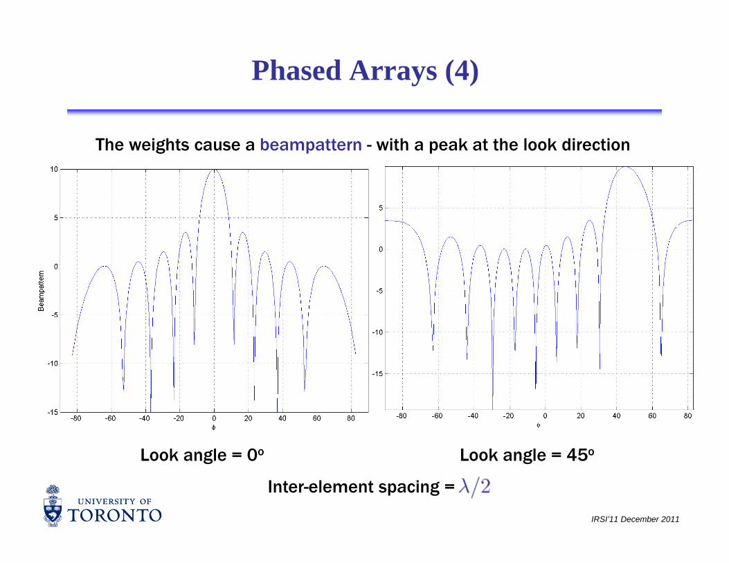
The weights cause a beampattern - with a peak at the look direction
Look angle = 0o Look angle = 45o
IRSI’11 December 2011
Look angle 0 Look angle 45
Inter-element spacing =
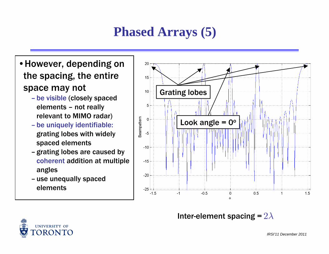
Phased Arrays (5)
•However, depending on the spacing, the entire p g,space may not
– be visible (closely spaced elements – not really
Grating lobes
relevant to MIMO radar)– be uniquely identifiable:
grating lobes with widely spaced elements
Look angle = 0o
spaced elements– grating lobes are caused by
coherent addition at multiple angles
– use unequally spaced elements
IRSI’11 December 2011
Inter-element spacing =
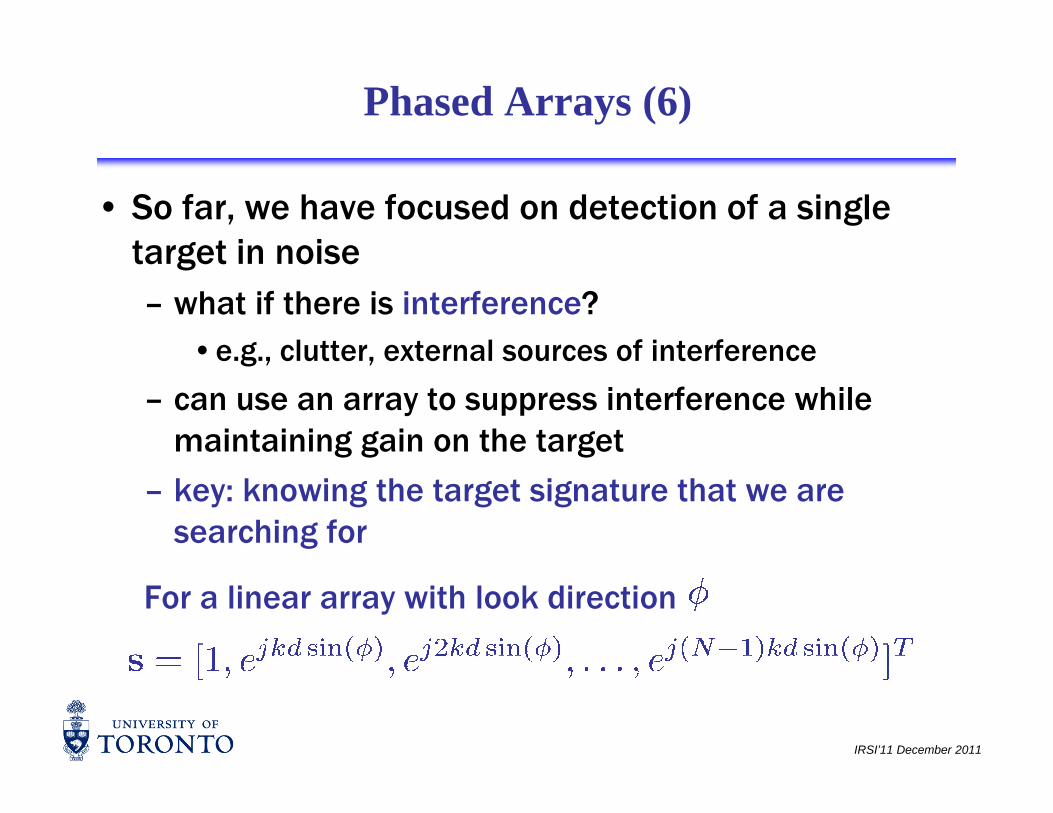
Phased Arrays (6)
• So far, we have focused on detection of a single target in noisetarget in noise– what if there is interference?
•e g clutter external sources of interferencee.g., clutter, external sources of interference
– can use an array to suppress interference while maintaining gain on the target
– key: knowing the target signature that we are searching for
For a linear array with look direction
IRSI’11 December 2011
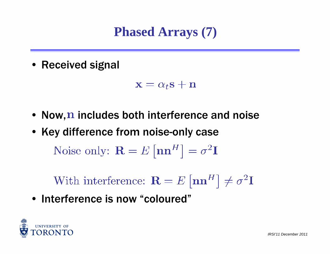
Phased Arrays (7)
• Received signal
N i l d b h i f d i• Now, includes both interference and noise
• Key difference from noise-only case
• Interference is now “coloured”
IRSI’11 December 2011
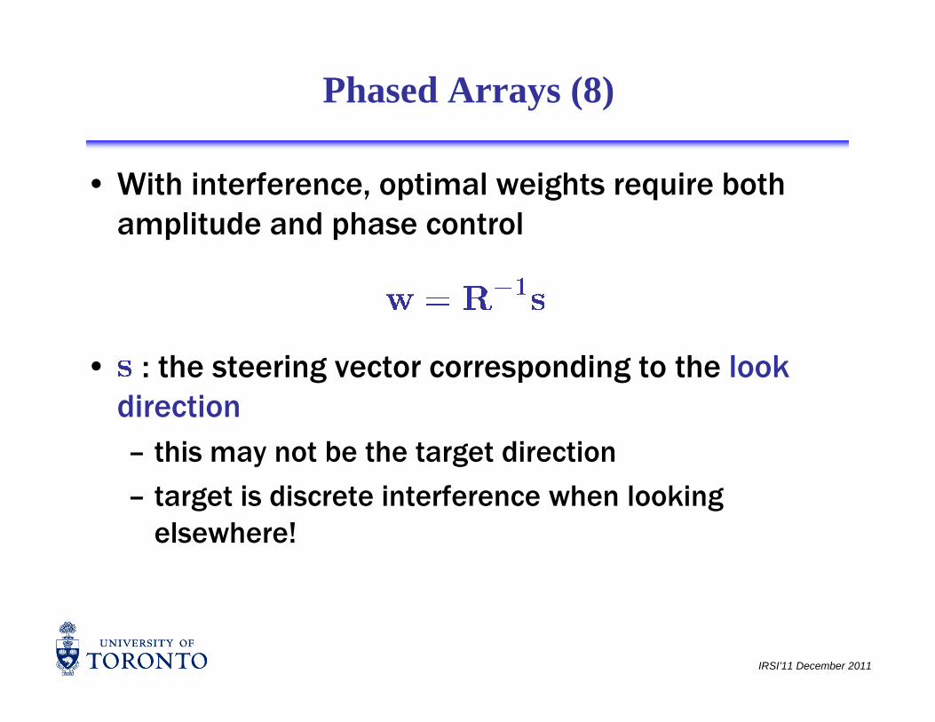
Phased Arrays (8)
• With interference, optimal weights require both amplitude and phase controlamplitude and phase control
• : the steering vector corresponding to the lookdirectiondirection– this may not be the target direction
– target is discrete interference when looking – target is discrete interference when looking elsewhere!
IRSI’11 December 2011
Phased Arrays (9)
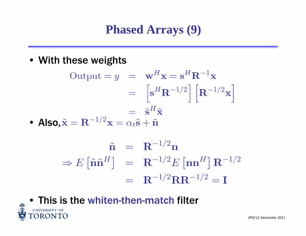
• With these weights
• Also,
IRSI’11 December 2011
• This is the whiten-then-match filter
Phased Arrays (10)
• The most important problem: the matrix is unknown a prioriunknown a priori– must be estimated using training data samples
– need at least samples – need at least samples
– these samples must •not contain any targetnot contain any target
•be “homogeneous”, i.e., statistically independent and identically distributed in relation to the interference
– usually, for each look range (the primary range cell) choose training data from range cells close by
l ll d d d t
IRSI’11 December 2011
•also called secondary data
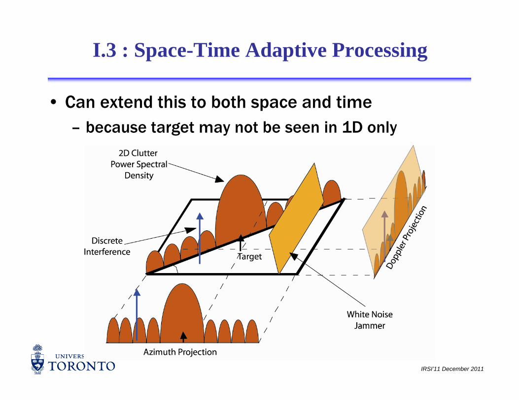
I.3 : Space-Time Adaptive Processing
• Can extend this to both space and timebecause target may not be seen in 1D only– because target may not be seen in 1D only
IRSI’11 December 2011
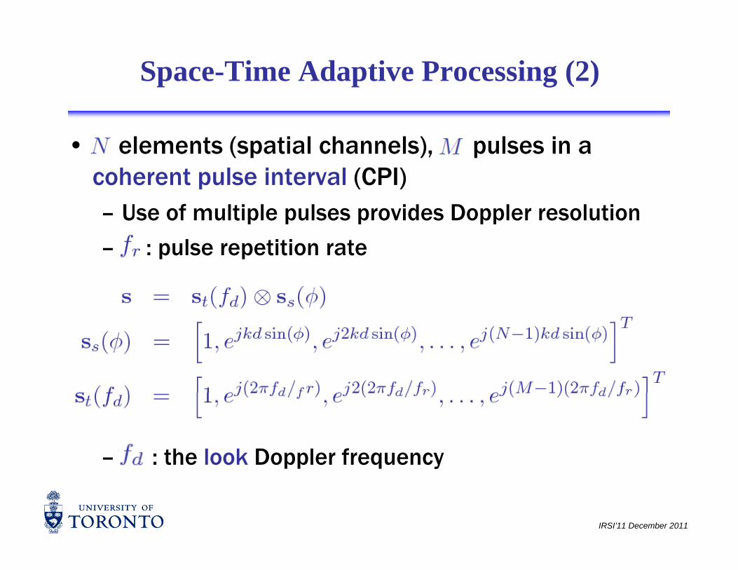
Space-Time Adaptive Processing (2)
• elements (spatial channels), pulses in a coherent pulse interval (CPI)coherent pulse interval (CPI)– Use of multiple pulses provides Doppler resolution
– : pulse repetition rate– : pulse repetition rate
– : the look Doppler frequency
IRSI’11 December 2011
t e oo opp e eque cy
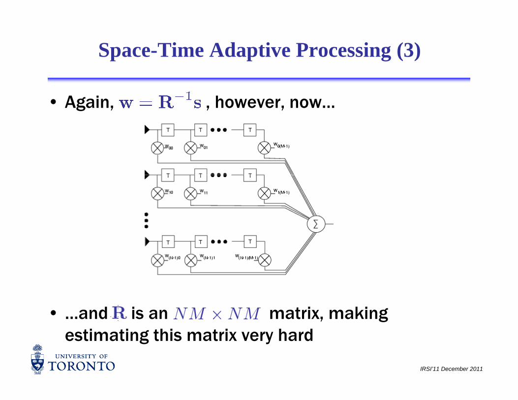
Space-Time Adaptive Processing (3)
• Again, , however, now…
• …and is an matrix, making
IRSI’11 December 2011
estimating this matrix very hard
Space-Time Adaptive Processing (4)
• To deal with estimation issues, usually one reduces the adaptive degrees of freedom (DoF) the adaptive degrees of freedom (DoF) – joint domain localized processing
•processing in a small region around look angle/Dopplerprocessing in a small region around look angle/Doppler
– Σ∆—STAP•Use sum (Σ) and difference (∆) channels only( ) ( ) y
– parametric adaptive matched filter•parametrize the matched filter
– fast fully adaptive processing•break large problem into a series of small problems
IRSI’11 December 2011
– many others

STAP (5): Reduced Rank STAP
• Several reduced rank methods can be described as
• Computational load is reduced by a factor of
• Required sample support– in practice, sample support is the fundamental
IRSI’11 December 2011
problem
Space-Time Adaptive Processing (6)
• In applying STAP in the real world, a non-homogeneity detector (NHD) is importanthomogeneity detector (NHD) is important– identifies samples within the secondary data set that
are statistically inconsistent are statistically inconsistent •these samples are discarded
• Several types of NHD in the literatureyp– all search for some kind of discriminant
• Reducing DoF coupled with NHD makes it possible to g p pimplement STAP
IRSI’11 December 2011
I.4 : Target Models
• Target amplitude a function of its radar cross section for complex targets a sum of returns from different – for complex targets, a sum of returns from different parts making the amplitude a random variable
• Swerling models:• Swerling models:– Type I: Amplitude Gaussian, independent scan-to-scan
– Type II: like type-I independent pulse-to-pulseType II: like type I, independent pulse to pulse
– Type III: One dominant, other smaller surfaces: constant plus Gaussian independent scan-to-scanp p
– Type IV: like type-III, independent pulse-to-pulse
– Type V: constant throughout
IRSI’11 December 2011
•best case
I.5 : Waveform Diversity
• Broad term covering waveform design and adapting waveforms in real-time to better improve waveforms in real-time to better improve detection/localization– generally try to improve signal-to-interference plus generally try to improve signal to interference plus
noise ratio
• “Diversity” implies having a choice of multiple y p g pwaveforms to achieve a specific purpose
• Start with waveform design…– …followed by MIMO radar…
– …followed by joint consideration of MIMO radar and
IRSI’11 December 2011
waveforms

A Brief History
• Waveform Diversityfirst discussions in late 1990s at AFRL Rome– first discussions in late 1990s at AFRL-Rome
– had spent 90s working on STAP and knowledge-based processingprocessing
– some work on joint design of waveforms and processing
– renewed interest in distributed aperturesrenewed interest in distributed apertures
• Work at AFRL and other place culminated in the 1st
Annual Waveform Diversity Workshop in Feb. 2003 y p– stayed “annual” until 2005 or so…
– was expanded into the series of Waveform Diversity and
IRSI’11 December 2011
p yDesign conferences
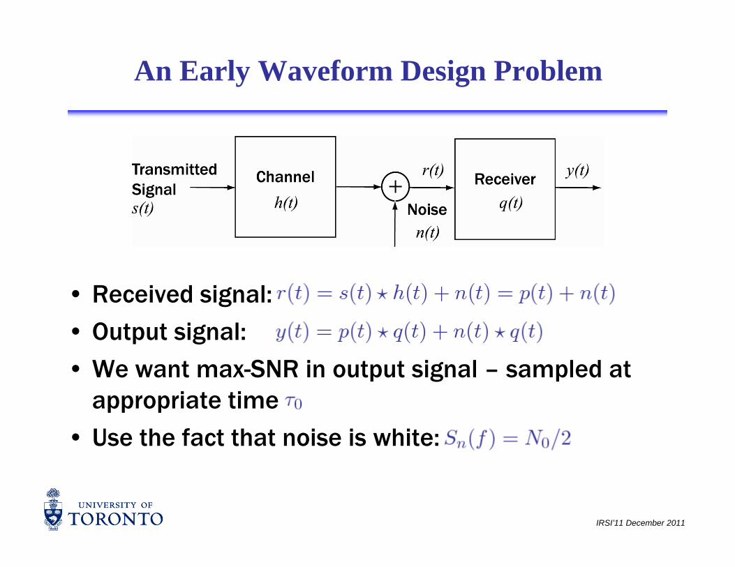
An Early Waveform Design Problem
• Received signal:
• Output signal:
• We want max-SNR in output signal – sampled at appropriate time
• Use the fact that noise is white:
IRSI’11 December 2011
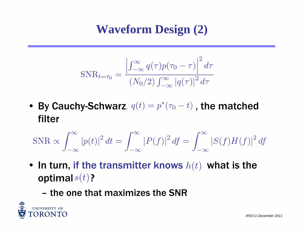
Waveform Design (2)
B C h S h h h d • By Cauchy-Schwarz, ,, the matched filter
f• In turn, if the transmitter knows , what is the optimal ?
th th t i i th SNR
IRSI’11 December 2011
– the one that maximizes the SNR
Waveform Design (3)
• This leads to an eigenvalue equation
hwhere
is the kernel of the channel
• This arises because of the magnitude squared term Sin the SNR
• Choose eigenfunction corresponding to largest
IRSI’11 December 2011
• If noise is coloured, whiten it first
Waveform Design (4)
• Need to normalize the energy to ensure the transmitter meets its power constrainttransmitter meets its power constraint
• So far, no limit on bandwidthincorporate bandwidth constraints by limiting the – incorporate bandwidth constraints by limiting the kernel function in the frequency domain
• Special case: flat channelSpecial case: flat channel– leads to prolate spheroidal wave functions
IRSI’11 December 2011
II : MIMO Radar
• Multiple Input Multiple Output radar systemsexploits multiple transmitters multiple receivers – exploits multiple transmitters, multiple receivers, multiple waveforms
•i.e., all available degrees of freedomi.e., all available degrees of freedom
– a generalization of multistatic radar
– let’s agree that MIMO radar research did not start in g2004
•called “multistatic radar”, “distributed apertures”, “waveform diversity”, “netted radar”….
•it is important to emphasize that MIMO radar research builds on previous works in this area
IRSI’11 December 2011
research builds on previous works in this area
MIMO Radar : Introduction (2)
• Statistical MIMO radar:often widely spaced apertures– often widely spaced apertures
•conceivably acts as one big aperture
– the target response for each transmit-receive pair is – the target response for each transmit-receive pair is statistically independent
•possibly due to different look angles or different p y gfrequencies
• Coherent MIMO radar– closely spaced apertures operating on the same
frequency, e.g., French RIAS system (1984)
ll i
IRSI’11 December 2011
– same target response to all tx-rx pairs
II.1 : Sample Result
Without Frequency Offset (No Diversity) With Frequency Offset (Waveform Diversity)
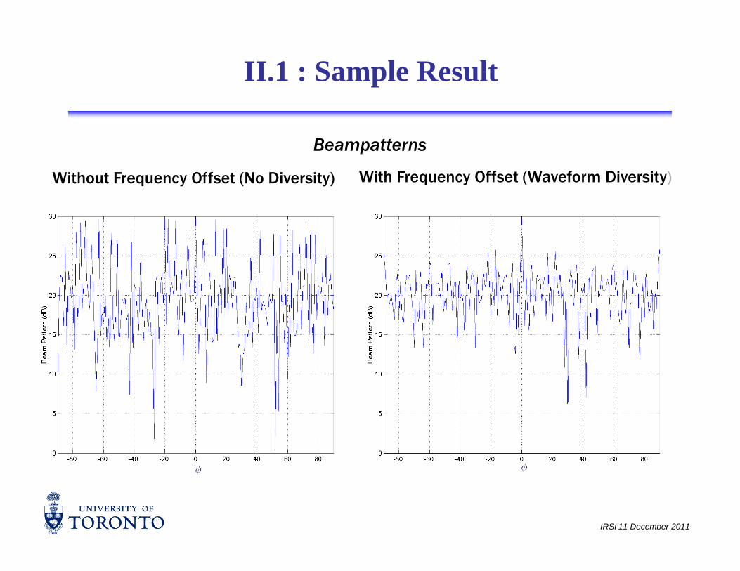
Beampatterns
Without Frequency Offset (No Diversity) With Frequency Offset (Waveform Diversity)
IRSI’11 December 2011
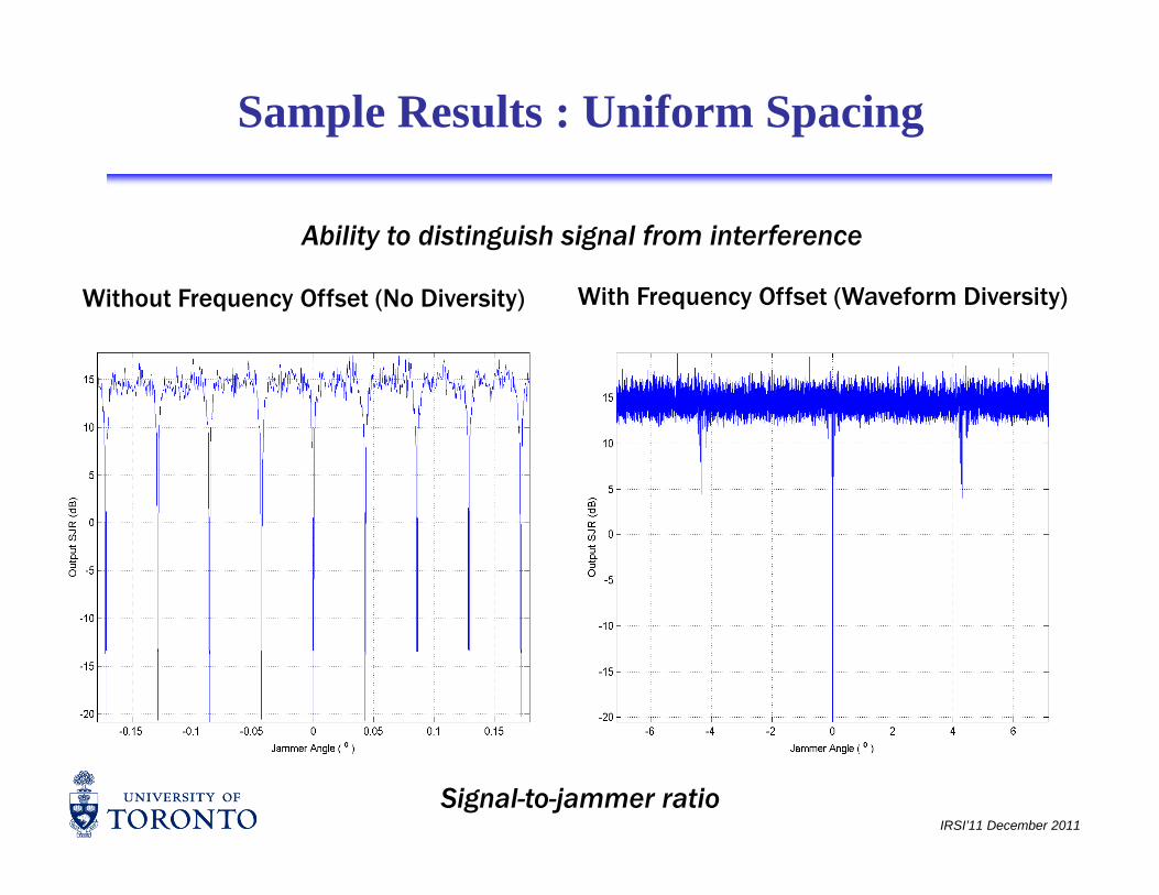
Sample Results : Uniform Spacing
Ability to distinguish signal from interference
Without Frequency Offset (No Diversity) With Frequency Offset (Waveform Diversity)
IRSI’11 December 2011
Signal-to-jammer ratio

II.2 Virtual Array Representation
• Consider transmit and receive antennastransmitters at – transmitters at
– receivers at
assume that the transmitters transmit orthogonal – assume that the transmitters transmit orthogonal coherent waveforms
•e.g., using orthogonal codes g , g g
•the receiver can distinguish each waveform without error
•after matching to the transmit signal at the receiver the received signal from target is
IRSI’11 December 2011
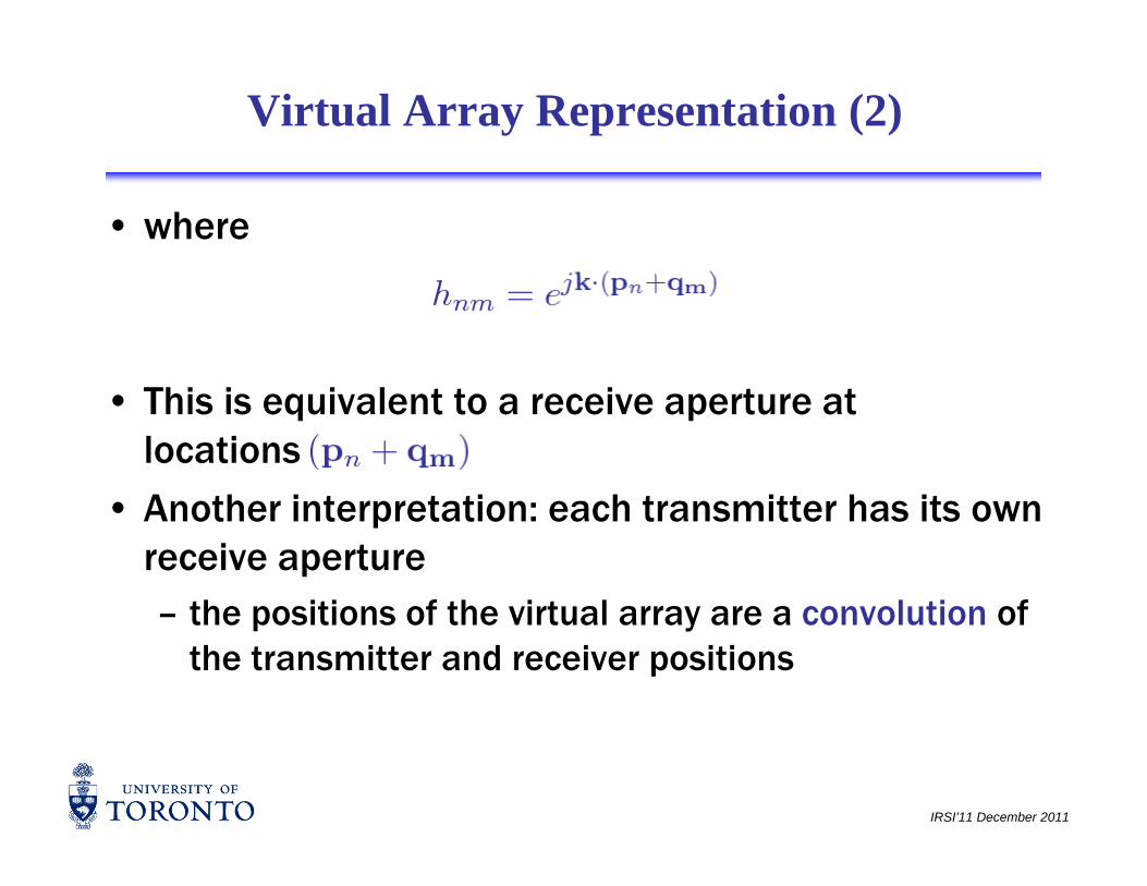
Virtual Array Representation (2)
• where
Thi i i l i • This is equivalent to a receive aperture at locations
A th i t t ti h t itt h it • Another interpretation: each transmitter has its own receive aperture
the positions of the virtual array are a convolution of – the positions of the virtual array are a convolution of the transmitter and receiver positions
IRSI’11 December 2011
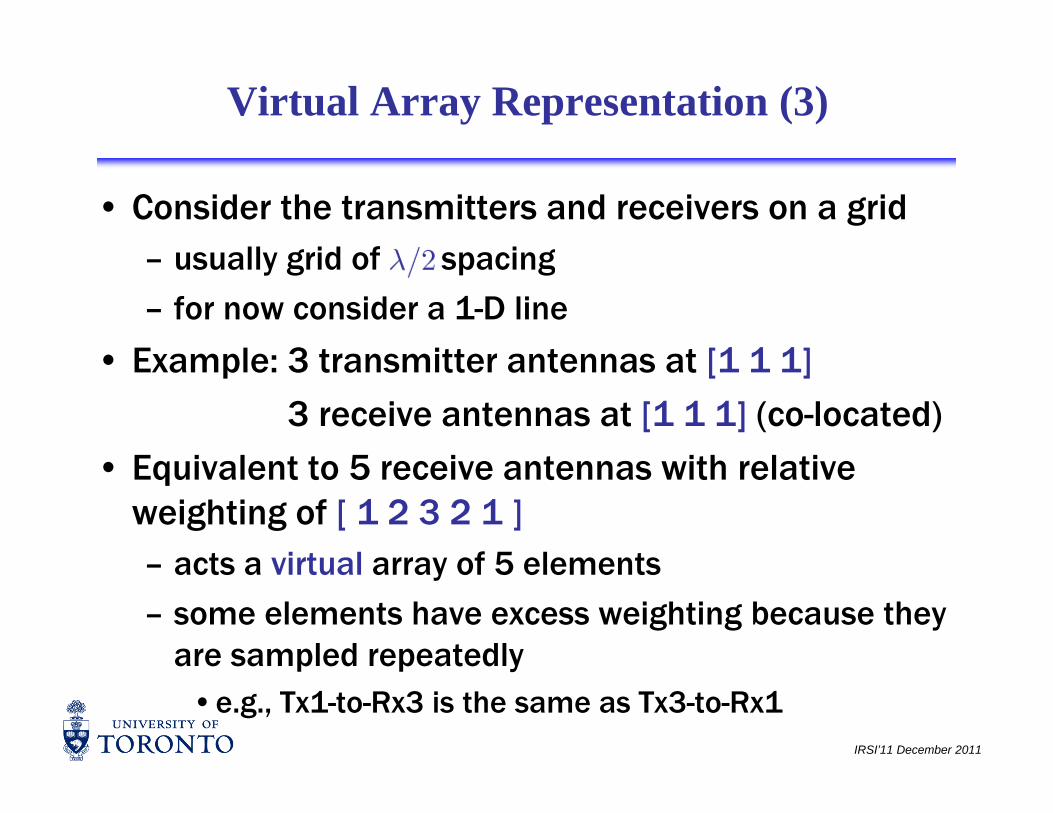
Virtual Array Representation (3)
• Consider the transmitters and receivers on a gridusually grid of spacing– usually grid of spacing
– for now consider a 1-D line
• Example: 3 transmitter antennas at [1 1 1]• Example: 3 transmitter antennas at [1 1 1]
3 receive antennas at [1 1 1] (co-located)
E i l t t 5 i t ith l ti • Equivalent to 5 receive antennas with relative weighting of [ 1 2 3 2 1 ]
acts a virtual array of 5 elements– acts a virtual array of 5 elements
– some elements have excess weighting because they are sampled repeatedly
IRSI’11 December 2011
are sampled repeatedly •e.g., Tx1-to-Rx3 is the same as Tx3-to-Rx1

Virtual Array Representation (4)
• Can be further improved by using a thinned array
E l 3 t l t t [1 1 0 1] d • Example: 3 antenna elements at [1 1 0 1] and co-located receive antennas results in a virtual array of [1 2 1 2 2 0 1] (a 6-element virtual array)[1 2 1 2 2 0 1] (a 6 element virtual array)
• Transmitter and receiver not necessarily co-located
• Example: 3 transmitter antennas at [1 1 1]• Example: 3 transmitter antennas at [1 1 1]
3 receive antennas at [1 0 0 1 0 0 1 0 0]
results in [ 1 1 1 1 1 1 1 1 1] (9 elements)results in [ 1 1 1 1 1 1 1 1 1] (9 elements)
• Here, there are no repeated paths and each transmit receive pair is unique
IRSI’11 December 2011
transmit-receive pair is unique
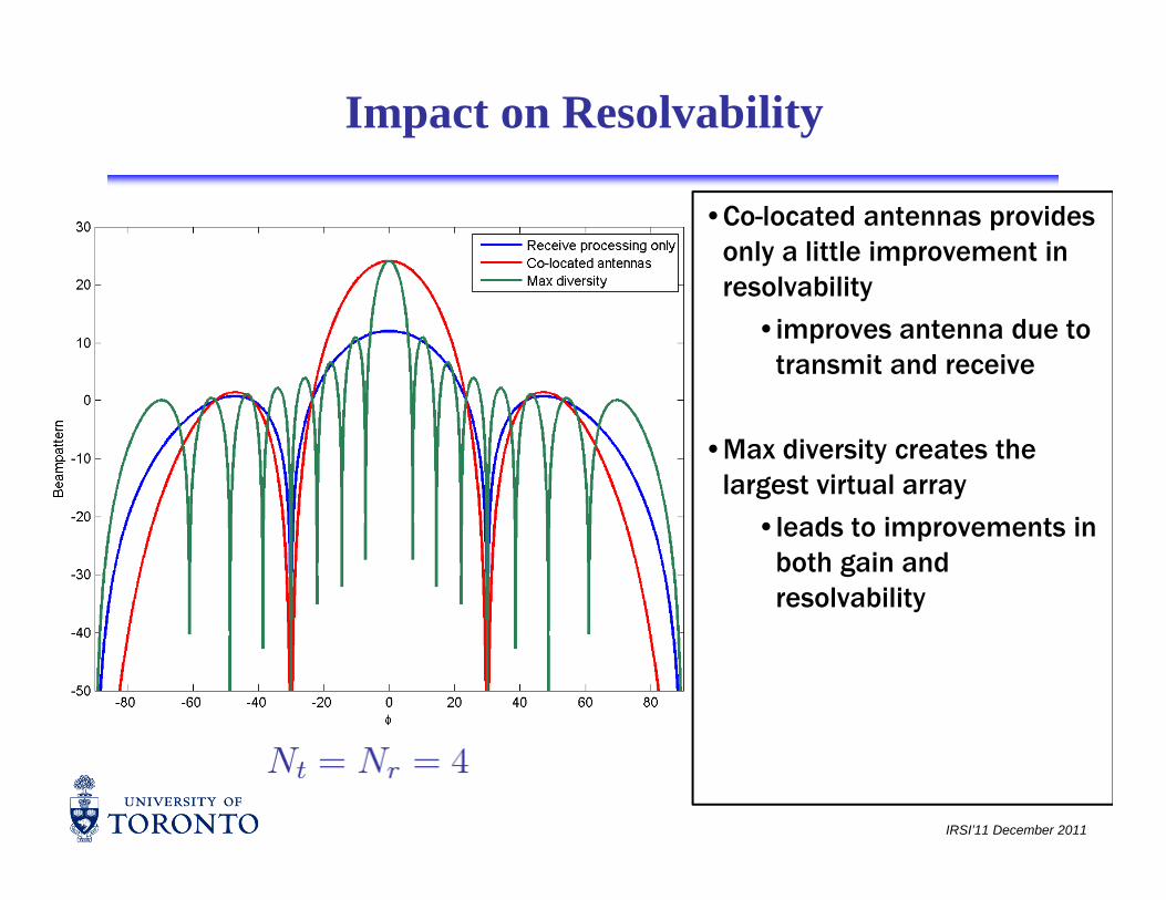
Impact on Resolvability
•Co-located antennas provides only a little improvement in
l bilit resolvability
•improves antenna due to transmit and receive
•Max diversity creates the largest virtual array
•leads to improvements in both gain and resolvability
IRSI’11 December 2011
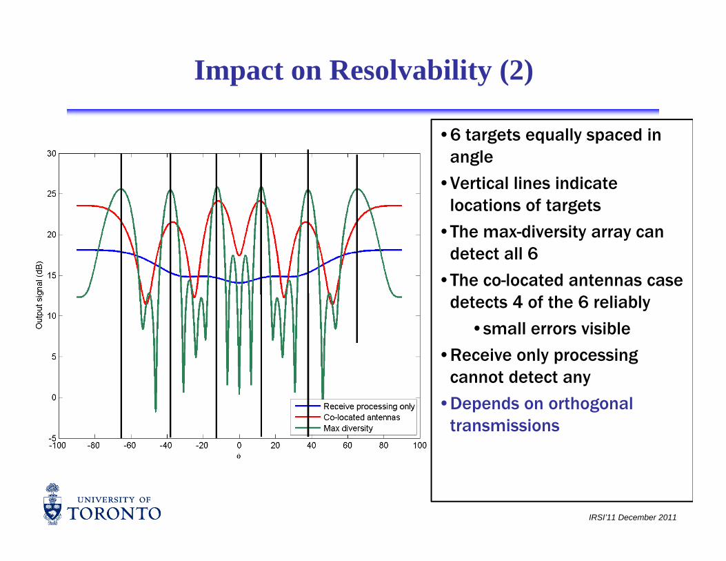
Impact on Resolvability (2)
•6 targets equally spaced in angle
•Vertical lines indicate locations of targets
•The max-diversity array can detect all 6
•The co-located antennas case detects 4 of the 6 reliably
•small errors visible
•Receive only processing cannot detect any
•Depends on orthogonal transmissions
IRSI’11 December 2011
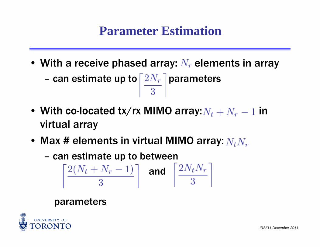
Parameter Estimation
• With a receive phased array: elements in arraycan estimate up to parameters– can estimate up to parameters
With l t d t / MIMO i • With co-located tx/rx MIMO array: in virtual array
• Max # elements in virtual MIMO array:• Max # elements in virtual MIMO array:– can estimate up to between
andand
parameters
IRSI’11 December 2011
parameters

II.3 : Theoretical Analysis
IRSI’11 December 2011How do we characterize such a system?

II.3.1 : Target Models
• In the case of co-located antennas, the target response is the same to all antennasresponse is the same to all antennas
• transmit antennas, receive antennas, pulses transmit antennas at– transmit antennas at
– receiver antennas at
– parameter vector for transmitter receiver :– parameter vector for transmitter , receiver :
– target at location: , velocity , parameters
– relative delay, relative Doppler,
IRSI’11 December 2011
relative delay, relative Doppler,

Target Models (2)
• Signal transmitted by antenna :
Sig l i d b t not
• Signal received by antenna : antenna index!
• : target amplitude seen at receiver due to ig l f t itt signal from transmitter
• Next step: matched filtering and samplingibl hi l h– possibly matching to pulse shapes
– pulses in a CPI
IRSI’11 December 2011
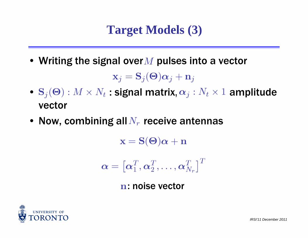
Target Models (3)
• Writing the signal over pulses into a vector
• : : signal matrix, amplitude vectorvector
• Now, combining all receive antennas
: noise vector
IRSI’11 December 2011
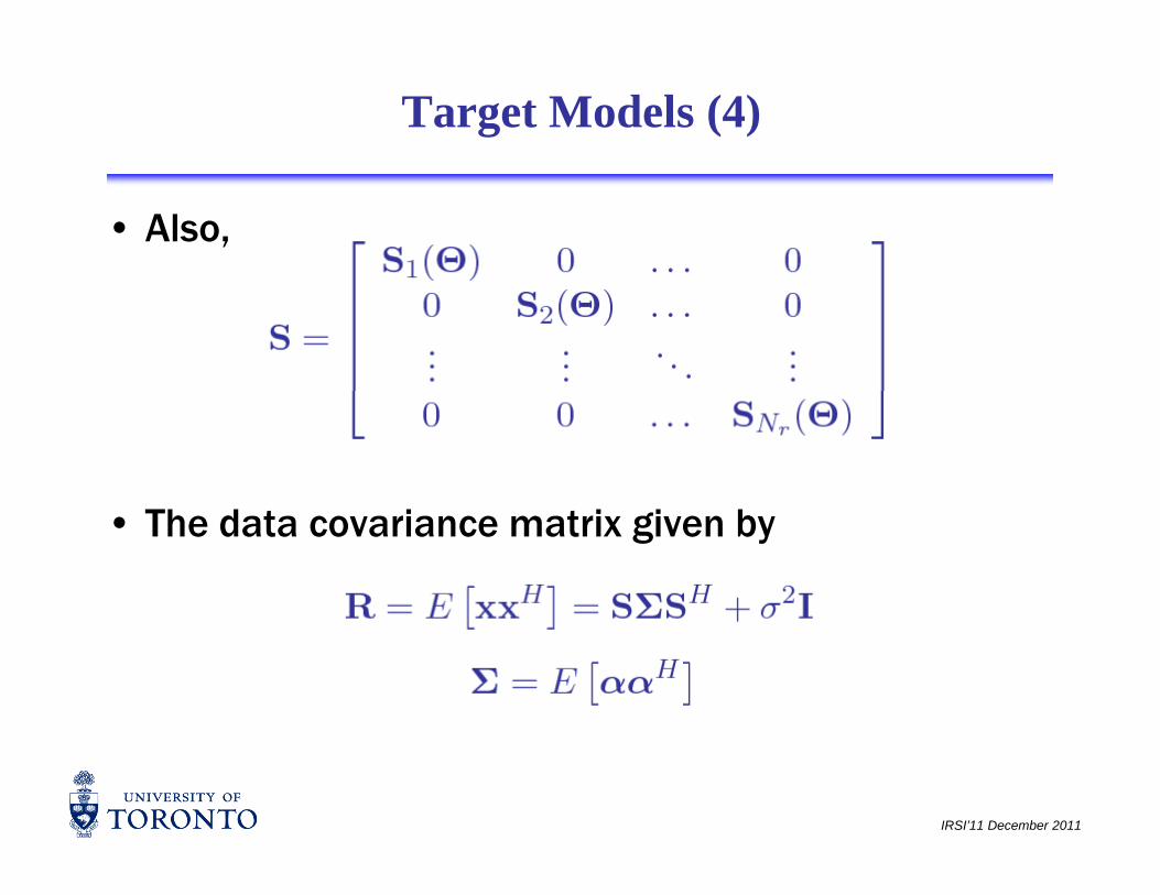
Target Models (4)
• Also,
• The data covariance matrix given by
IRSI’11 December 2011
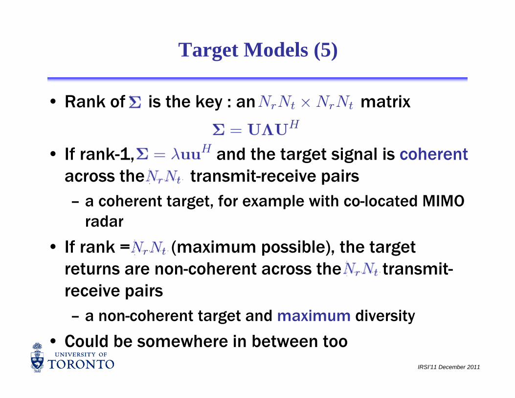
Target Models (5)
• Rank of is the key : an matrix
• If rank-1, and the target signal is coherentacross the transmit receive pairsacross the transmit-receive pairs– a coherent target, for example with co-located MIMO
radarradar
• If rank = (maximum possible), the target returns are non-coherent across the transmit-returns are non coherent across the transmitreceive pairs– a non-coherent target and maximum diversity
IRSI’11 December 2011
• Could be somewhere in between too

II.3.2 : Diversity Order
• In wireless communications, diversity order measures the number of independent paths in measures the number of independent paths in multi-antenna systems– slope of the BER v/s SNR curve at high SNRslope of the BER v/s SNR curve at high SNR
– usually achieved at moderate SNR regime
• Can we use this idea in MIMO radar systems?Can we use this idea in MIMO radar systems?
• A few concerns:– High SNR is irrelevant in radar systemsHigh SNR is irrelevant in radar systems
– Probabilities of detection/miss only make sense if false alarm is kept constant
IRSI’11 December 2011
– The rising part of the PD curve is of most interest
Background
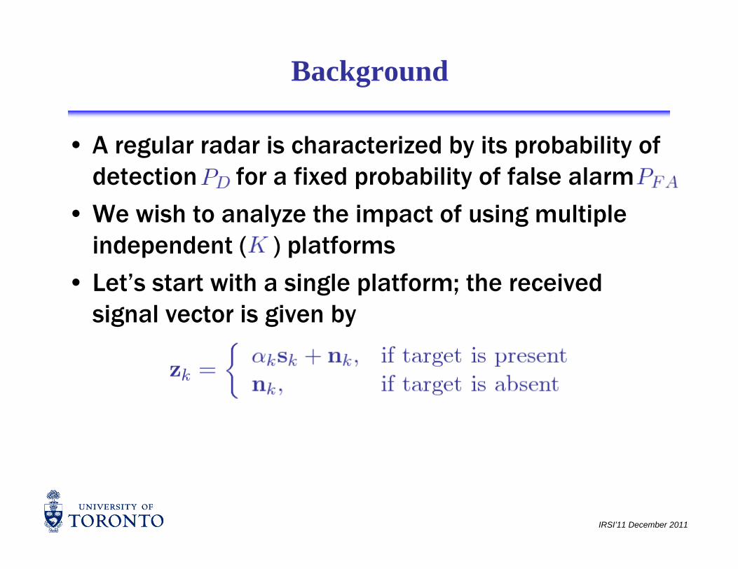
• A regular radar is characterized by its probability of detection for a fixed probability of false alarmdetection for a fixed probability of false alarm
• We wish to analyze the impact of using multiple independent ( ) platformsindependent ( ) platforms
• Let’s start with a single platform; the received signal vector is given bysignal vector is given by
IRSI’11 December 2011
Background (2)
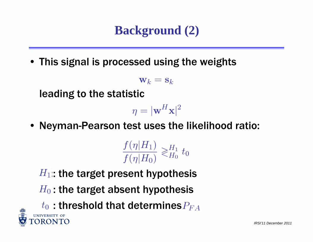
• This signal is processed using the weights
leading to the statistic
• Neyman-Pearson test uses the likelihood ratio:
:: the target present hypothesis
: the target absent hypothesis
IRSI’11 December 2011
: threshold that determines
Background (3)
• Under , is exponentially distributed with mean andand
• Similarly under isis exponentially distributed • Similarly, under , isis exponentially distributed with mean and
• Note that reducing the threshold (increasing sensitivity) increases both and sensitivity) increases both and
• As we use a MIMO radar, the analysis must account for this increase in both measures
IRSI’11 December 2011
for this increase in both measures
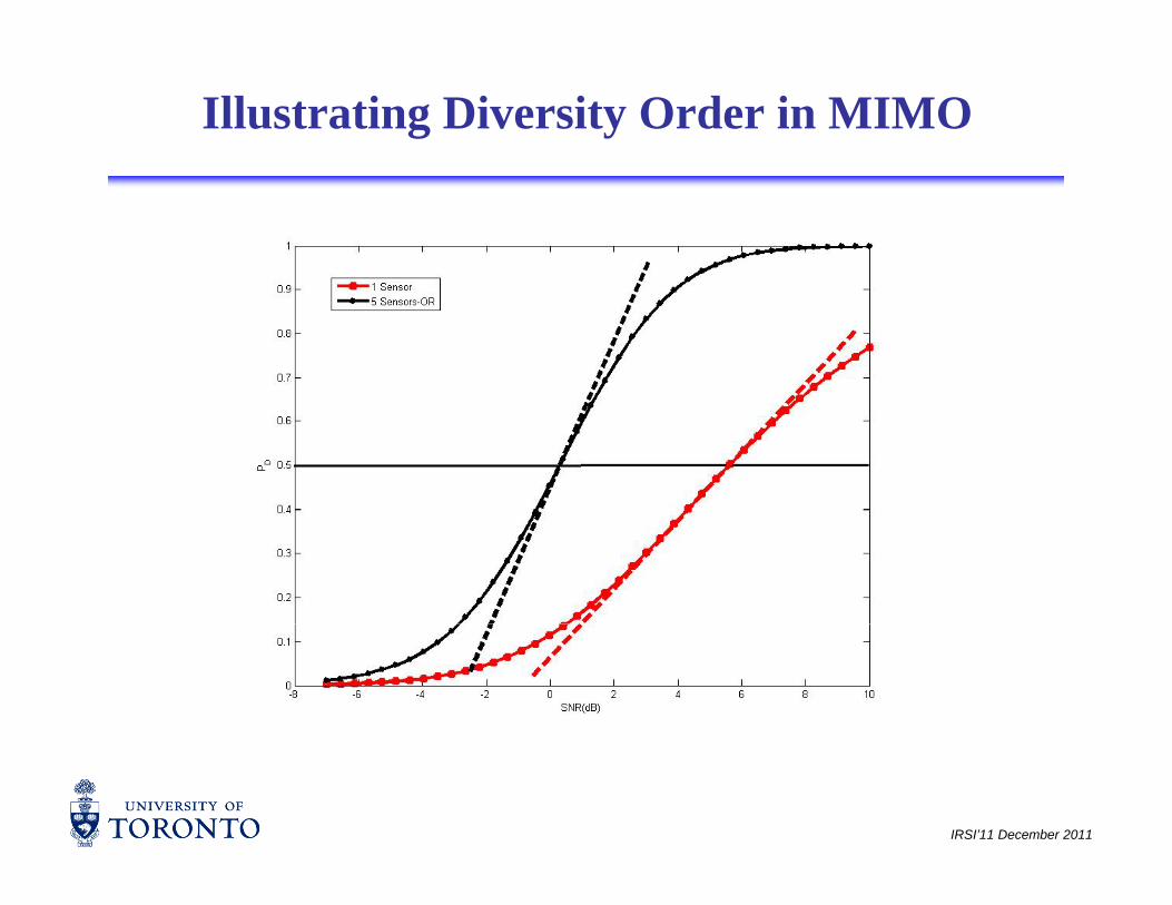
Illustrating Diversity Order in MIMO
IRSI’11 December 2011
Diversity Order : Definition
• Our definition also uses a slope:
The diversity order of a radar system is the slope in a linear scale of the probability of detection versus SNR linear scale of the probability of detection versus SNR
curve at for a fixed probability of false alarm.
• Definition captures– the SNR range of interestg
– is valid only for a fixed false alarm rate
– the interaction of the spatial degrees of freedom and
IRSI’11 December 2011
p gprocessing scheme
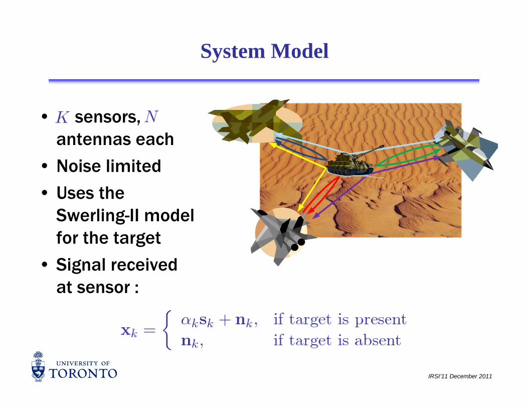
System Model
• sensors, antennas each
• Noise limited
• Uses the Swerling-II model for the target
• Signal received t at sensor :
IRSI’11 December 2011
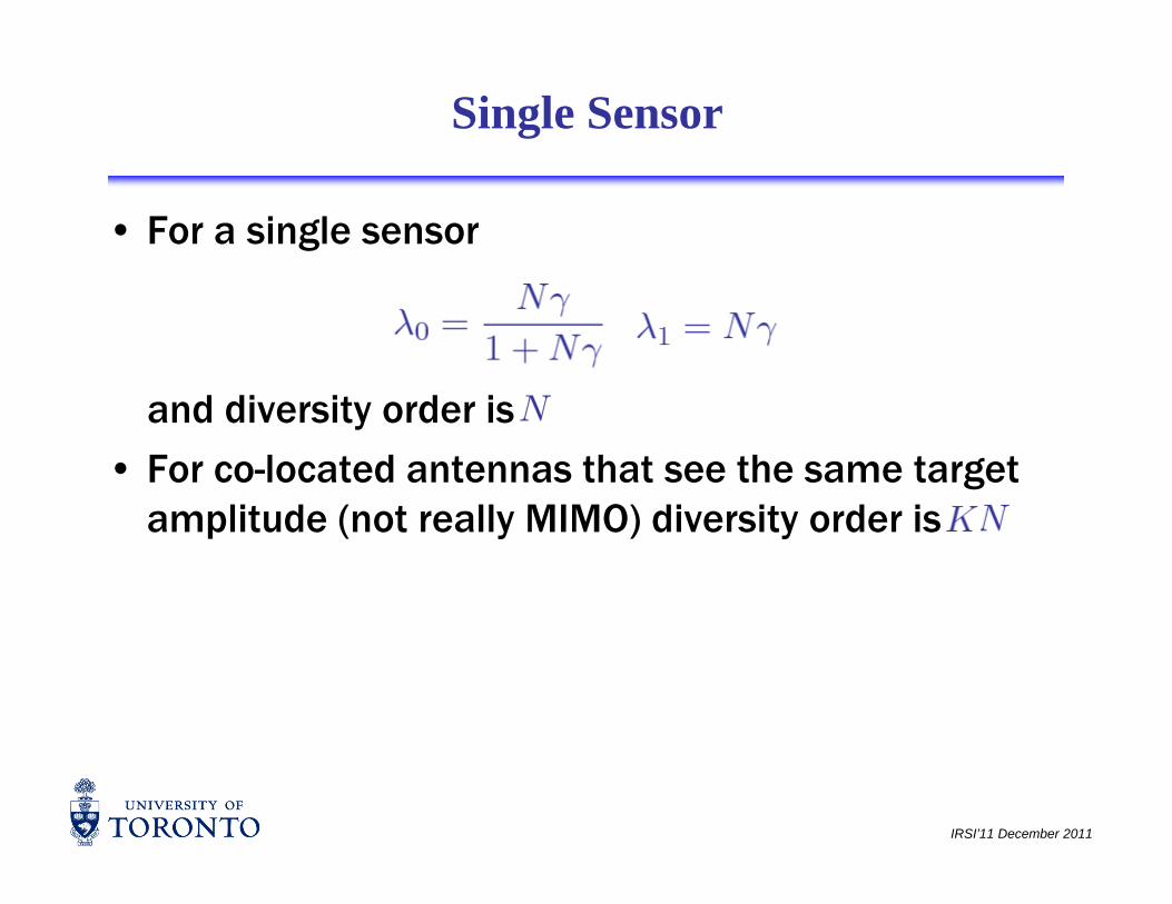
Single Sensor
• For a single sensor
d di i d i and diversity order is
• For co-located antennas that see the same target lit d ( t ll MIMO) di it d i amplitude (not really MIMO) diversity order is
IRSI’11 December 2011

Joint Detection
• Each sensor transmits its exact likelihood ratio to a fusion centerfusion center– the fusion center combines the LR from all sensors
•the LR are proportional to signal powerthe LR are proportional to signal power
•similar to maximal ratio combining in communications
– each sensor contributes an exponential RVp•the sum follows a gamma distribution
IRSI’11 December 2011
Joint Detection (2)
• PDF under provides the threshold by finding the false alarm rate ( )false alarm rate ( )
• PDF under then finds
• For large the diversity order proportional to• For large , the diversity order proportional to
• The improved detection probability is partiallyoffset by increased false alarm rate offset by increased false alarm rate
IRSI’11 December 2011
Distributed Detection
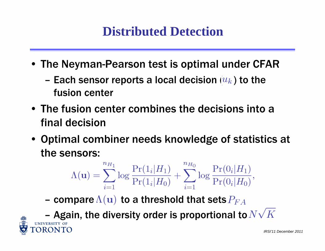
• The Neyman-Pearson test is optimal under CFAREach sensor reports a local decision ( ) to the – Each sensor reports a local decision ( ) to the fusion center
• The fusion center combines the decisions into a • The fusion center combines the decisions into a final decision
• Optimal combiner needs knowledge of statistics at Optimal combiner needs knowledge of statistics at the sensors:
– compare to a threshold that sets
IRSI’11 December 2011
– Again, the diversity order is proportional to
Distributed Detection (2)
• More practically, OR AND MAJ rules– OR, AND, MAJ rules
• OR rule: the diversity order is proportional to
AND l th di it d i ti l t • AND rule: the diversity order is proportional to – there is no gain due to distributed sensors
th d d d t ti b bilit i ff t tl b – the reduced detection probability is offset exactly by the reduced false alarm rate
• MAJ rule: somewhere in between• MAJ rule: somewhere in between
IRSI’11 December 2011
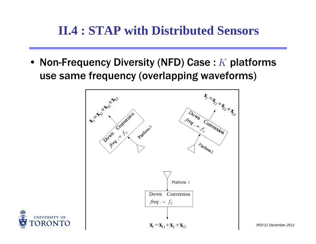
II.4 : STAP with Distributed Sensors
• Non-Frequency Diversity (NFD) Case : platforms use same frequency (overlapping waveforms)use same frequency (overlapping waveforms)
IRSI’11 December 2011
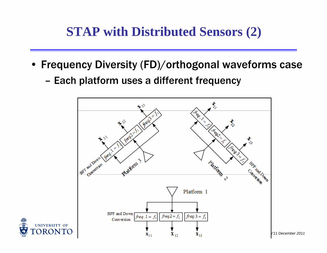
STAP with Distributed Sensors (2)
• Frequency Diversity (FD)/orthogonal waveforms caseEach platform uses a different frequency – Each platform uses a different frequency
IRSI’11 December 2011
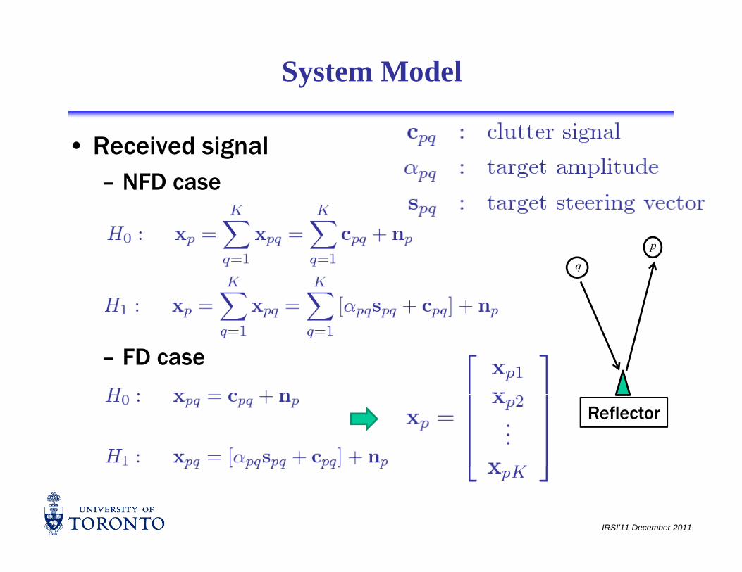
System Model
• Received signalNFD case– NFD case
pp
q
– FD case
Reflector
IRSI’11 December 2011

Interference Covariance Matrix
• Define
NFD • NFD case
• FD case
IRSI’11 December 2011
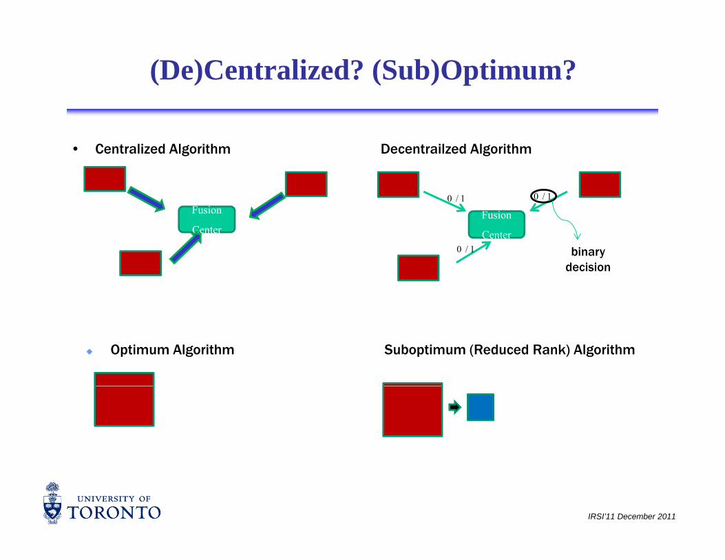
(De)Centralized? (Sub)Optimum?
• Centralized Algorithm Decentrailzed Algorithm
Fusion
CenterFusion
Center
1/0 1/0
binary decision
1/0
Optimum Algorithm Suboptimum (Reduced Rank) Algorithm
IRSI’11 December 2011
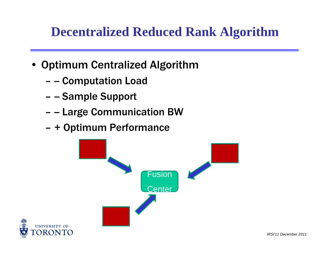
Decentralized Reduced Rank Algorithm
• Optimum Centralized AlgorithmComputation Load– -- Computation Load
– -- Sample Support
Large Communication BW– -- Large Communication BW
– + Optimum Performance
FusionFusion
Center
IRSI’11 December 2011
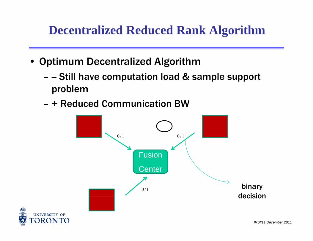
Decentralized Reduced Rank Algorithm
• Optimum Decentralized AlgorithmStill have computation load & sample support – -- Still have computation load & sample support
problem
– + Reduced Communication BW+ Reduced Communication BW
1/0 1/0
Fusion
C t
1/0 1/0
Center
1/0 binary decision
IRSI’11 December 2011
decision

Decentralized Reduced Rank Algorithm
• Sub-Optimum Decentralized AlgorithmPerformance Degradation– -- Performance Degradation
– + Reduced Computation Load
+ Reasonable Sample Support– + Reasonable Sample Support
Fusion
1/01/0
Center
1/0 binary
IRSI’11 December 2011
decision
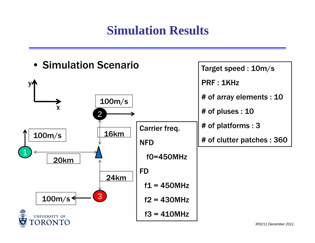
Simulation Results
• Simulation Scenario Target speed : 10m/s
100m/sx
y PRF : 1KHz
# of array elements : 10
2
100m/s 16kmCarrier freq.
x
# of pluses : 10
# of platforms : 3
1
100m/s
20km
NFD
f0=450MHz
# of clutter patches : 360
3100m/s
24kmFD
f1 = 450MHz
f2 430MH
IRSI’11 December 2011
3100m/s f2 = 430MHz
f3 = 410MHz
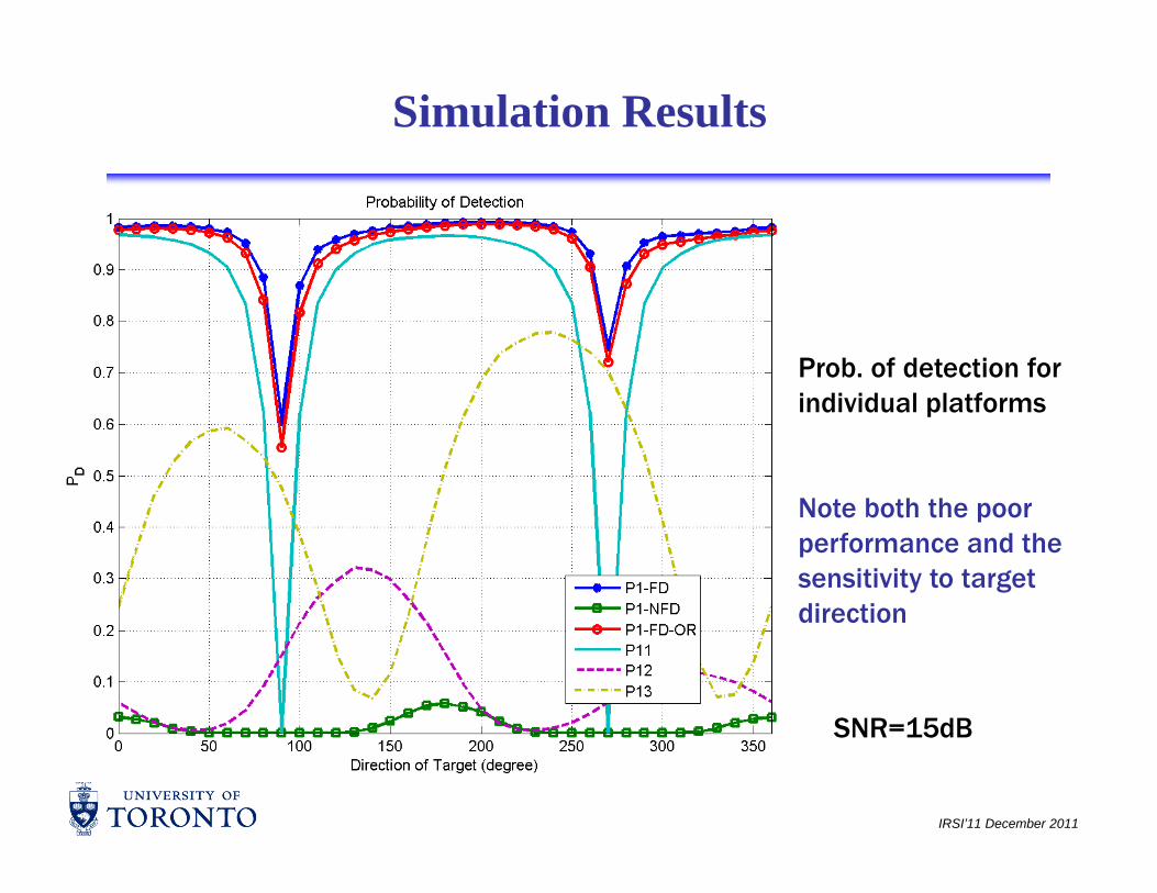
Simulation Results
Prob. of detection for individual platforms
Note both the poor Note both the poor performance and the sensitivity to target directiondirection
SNR=15dB
IRSI’11 December 2011
SNR=15dB
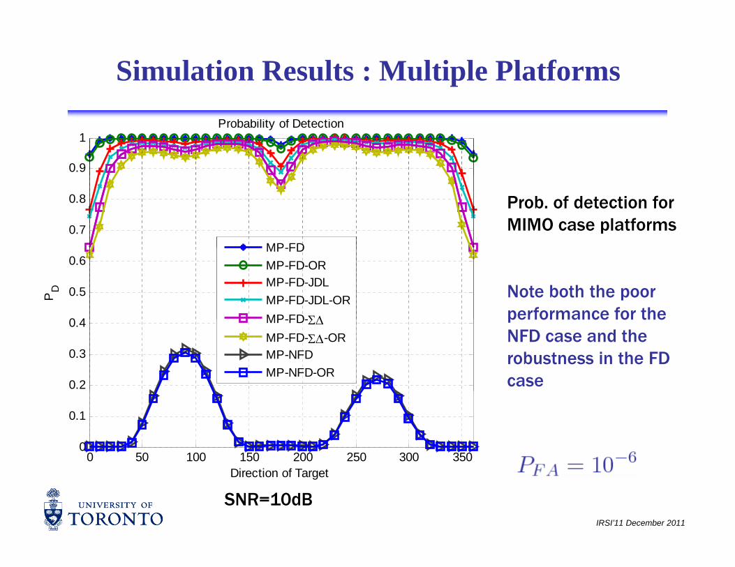
Simulation Results : Multiple Platforms
0.9
1Probability of Detection
0.7
0.8
MP-FD
Prob. of detection for MIMO case platforms
0 4
0.5
0.6
PD
MP-FDMP-FD-ORMP-FD-JDLMP-FD-JDL-ORMP-FD-Σ∆
Note both the poor performance for the
0.2
0.3
0.4 MP-FD-Σ∆MP-FD-Σ∆-ORMP-NFDMP-NFD-OR
performance for the NFD case and the robustness in the FD case
0 50 100 150 200 250 300 3500
0.1
IRSI’11 December 2011
SNR=10dB
Direction of Target
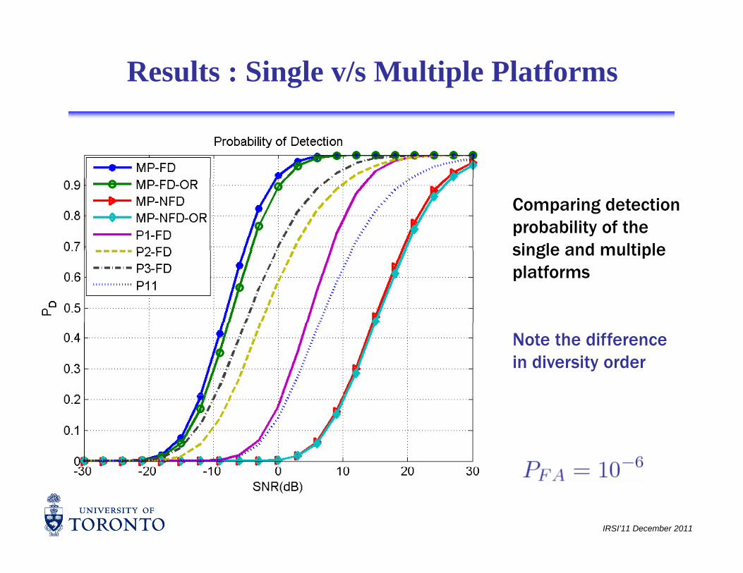
Results : Single v/s Multiple Platforms
Comparing detection probability of the single and multiple single and multiple platforms
Note the difference in diversity order
IRSI’11 December 2011

Results : Multiple Platforms
MP-FDMP FD OR
0.7
0.8
0.9 MP-FD-ORMP-FD-JDLMP-FD-JDL-ORMP-FD-Σ∆MP-FD-Σ∆-OR
Comparing detection probability of different processing
0.4
0.5
0.6
PD
MP-NFDMP-NFD-OR schemes
0.2
0.3
0.4Note they all appear to have the same diversity order
-30 -20 -10 0 10 20 300
0.1
SNR
IRSI’11 December 2011
Discussion : Diversity Order
• There is no loss in diversity due to using a sub-optimum STAP approachoptimum STAP approach– the JDL and Σ∆ approaches have curves that are
parallelparallel
– appears to have the same diversity order as the fully adaptive, centralized, scheme
•though theoretically, asymptotically in : – centralized scheme: ;
distributed OR scheme: – distributed OR scheme:
• Clear loss in diversity for the NFD scheme
IRSI’11 December 2011
y
Discussion : Issues Not Addressed
• The results shown here – and most research in MIMO systems – are based on a key assumptionMIMO systems – are based on a key assumption– synchronization across platforms
– in radar each sample corresponds to range bin– in radar, each sample corresponds to range bin•in processing across multiple platforms, a key
assumption is that the samples at a specific time at all platforms refers to the same range bin
– this is crucial also for secondary data in STAP for MIMO radar
•essentially, in these results, we have assumed true time delay
IRSI’11 December 2011
Part III : MIMO and Waveform Diversity
• So far we have considered detection and estimation using a MIMO radarestimation using a MIMO radar– no discussion of the choice of waveform
– first deal with case without constraints and then we – first deal with case without constraints and then we will add some practical constraints
• MIMO ambiguity functionMIMO ambiguity function– generalization of the ambiguity function to MIMO
– interpret the ambiguity function as the cross-p g ycorrelation between estimating the true target parameters and test parameters
IRSI’11 December 2011
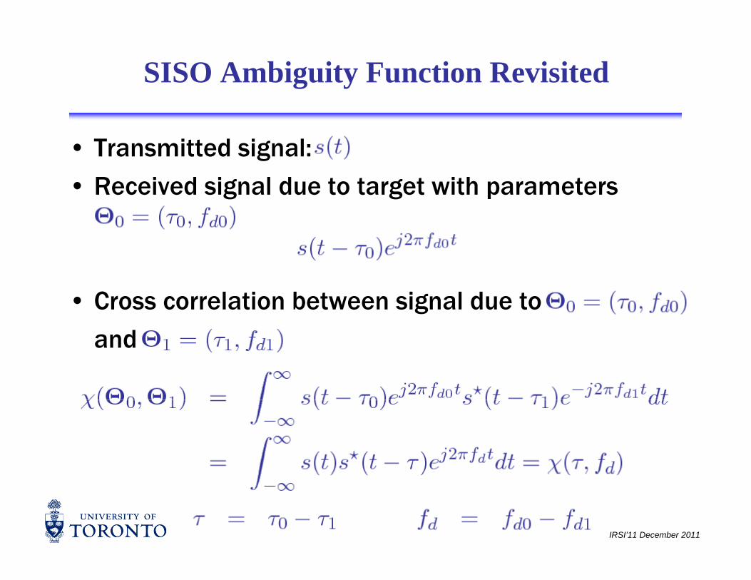
SISO Ambiguity Function Revisited
• Transmitted signal:
R i d ig l d t t g t ith t• Received signal due to target with parameters
• Cross correlation between signal due to
and
IRSI’11 December 2011
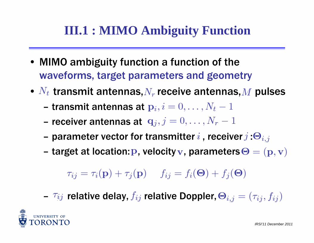
III.1 : MIMO Ambiguity Function
• MIMO ambiguity function a function of the waveforms target parameters and geometrywaveforms, target parameters and geometry
• transmit antennas, receive antennas, pulses transmit antennas at– transmit antennas at
– receiver antennas at
– parameter vector for transmitter receiver :– parameter vector for transmitter , receiver :
– target at location: , velocity , parameters
– relative delay, relative Doppler,
IRSI’11 December 2011
relative delay, relative Doppler,
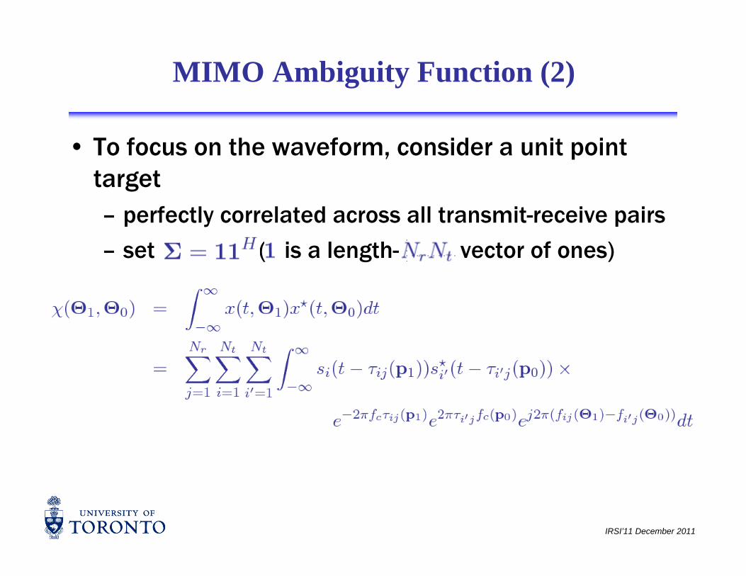
MIMO Ambiguity Function (2)
• To focus on the waveform, consider a unit point targettarget– perfectly correlated across all transmit-receive pairs
– set ( is a length- vector of ones) – set ( is a length- vector of ones)
IRSI’11 December 2011
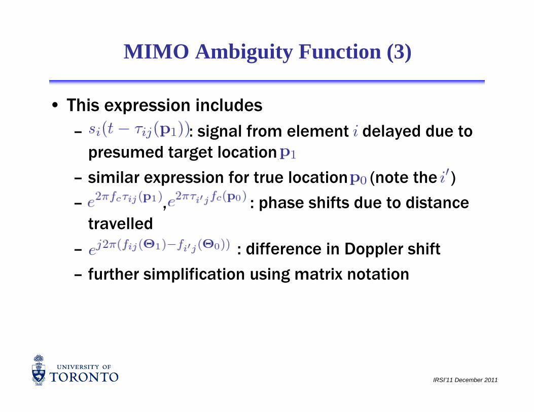
MIMO Ambiguity Function (3)
• This expression includes signal from element delayed due to – : signal from element delayed due to
presumed target location
– similar expression for true location (note the ) similar expression for true location (note the )
– , : phase shifts due to distance travelled
– : difference in Doppler shift
– further simplification using matrix notation
IRSI’11 December 2011
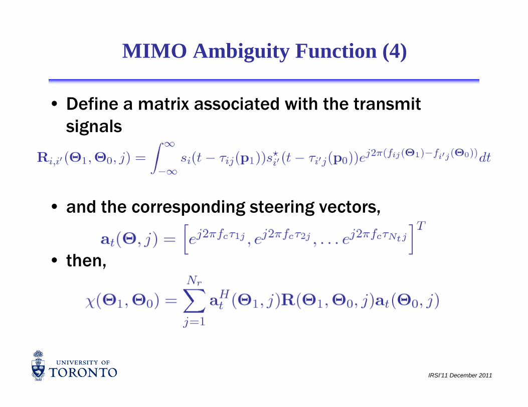
MIMO Ambiguity Function (4)
• Define a matrix associated with the transmit signalssignals
• and the corresponding steering vectors,
• then,
IRSI’11 December 2011
MIMO Ambiguity Function (5)
• Note that the ambiguity function is a complicated function of the geometry of the transmit-receive function of the geometry of the transmit-receive arrays– and depends on the target modeland depends on the target model
• Also, there is no free lunch– let . The “clear” area that can be created in let . The clear area that can be created in
delay-Doppler space is reduced by a factor of (work of Y. Abramovich and G. Frazer)
IRSI’11 December 2011
III.2 : MIMO Waveform Design
• Many different approachescovariance matrix design– covariance matrix design
– in frequency domain
max mutual information/MMSE– max. mutual information/MMSE
– with and without clutter statistics
IEEE search for ‘waveform design <and> MIMO – IEEE search for waveform design <and> MIMO radar’ results in 157 choices!
IRSI’11 December 2011
MIMO Waveform Design (2)
• transmit antennas, receive antennas, pulses simple case point transmitters and receivers– simple case: point transmitters and receivers
– transmitter transmits
• In continuous time target response between • In continuous time, target response between transmitter and receiver :
• In discrete time signal component at element• In discrete time, signal component at element
• : observation window
IRSI’11 December 2011
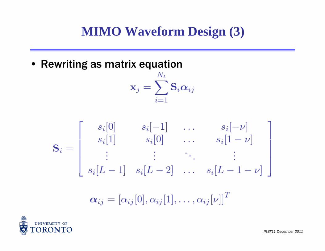
MIMO Waveform Design (3)
• Rewriting as matrix equation
IRSI’11 December 2011
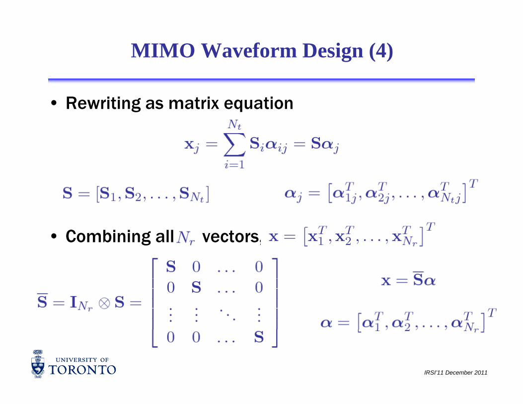
MIMO Waveform Design (4)
• Rewriting as matrix equation
• Combining all vectors,
IRSI’11 December 2011

MIMO Waveform Design (5)
• MMSE estimate : given find the minimum mean squared error estimate of squared error estimate of – given MMSE estimate is well known
• Optimal waveform: find the waveform ( ) that Optimal waveform: find the waveform ( ) that minimizes this MMSE– however we must meet a power constraint
IRSI’11 December 2011
p

MIMO Waveform Design (6)
• The optimization problem is
• : energy available per time-slot over all transmitters
G f• Generally requires an eigenvalue decomposition of – transmit on the eigenvectors of
IRSI’11 December 2011
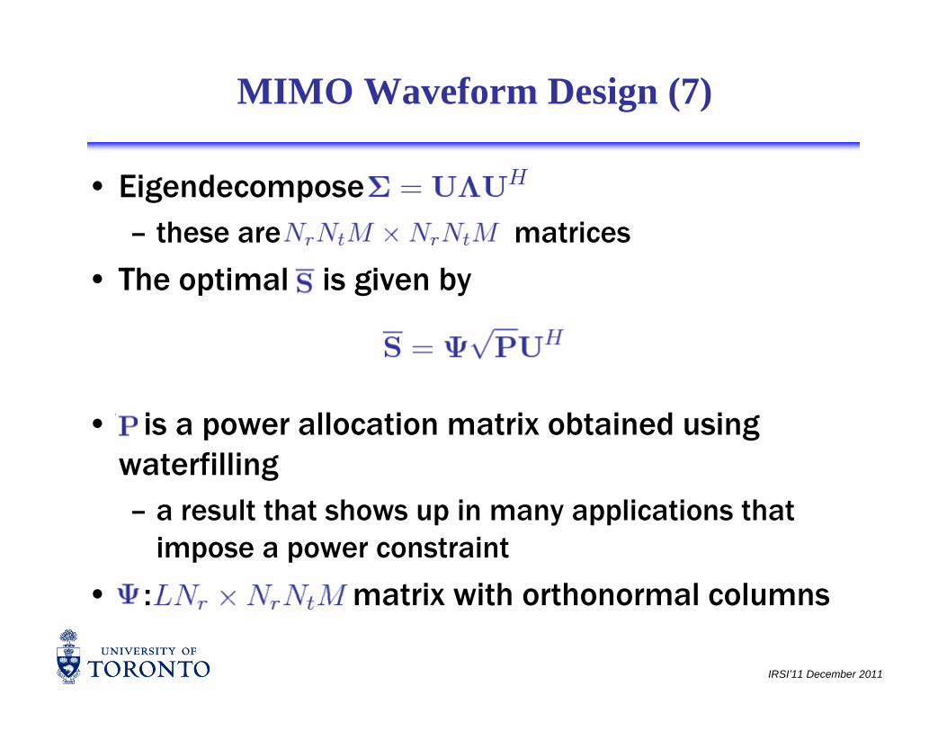
MIMO Waveform Design (7)
• Eigendecomposethese are matrices– these are matrices
• The optimal is given by
• is a power allocation matrix obtained using waterfilling
lt th t h i li ti th t – a result that shows up in many applications that impose a power constraint
• : matrix with orthonormal columns
IRSI’11 December 2011
• : matrix with orthonormal columns

MIMO Waveform Design (8)
• The key is the power allocation matrix
Effective noise level of Channel 1
IRSI’11 December 2011

MIMO Waveform Design (9)
• is the “water level”, chosen such that
Note that some “channels” are too weak to be
ll t d allocated power
IRSI’11 December 2011
MIMO Waveform Design (10)
• This is a first cut at optimize waveformsassumes target statistics are known– assumes target statistics are known
– other than power constraint, no other constraints
assumes perfect synchronization– assumes perfect synchronization
– ignores interference
• Each of these issues has been addressed in the • Each of these issues has been addressed in the literature– constant modulus waveforms waveforms formed by constant modulus waveforms, waveforms formed by
a chosen basis set, etc. etc.
– furthermore, other optimization criteria are also
IRSI’11 December 2011
, pconsidered, e.g., mutual information
III.3 : Fast-Time & Slow-Time MIMO
• MIMO waveforms still see the same total “amount” of range-Doppler spaceof range-Doppler space– fast-time versus slow-time MIMO
•in fast-time use time-staggered waveformsin fast time, use time staggered waveforms– reduction in PRF implies reduction in unambiguous Doppler
•in slow-time use Doppler-shifted waveforms– this reduces the unambiguous Doppler
•which is better depends on your application
i t t ith th k f Ab i h d F– consistent with the work of Abramovich and Frazer
• Focus here on a single-receive antenna ( )t it t l i CPI b f
IRSI’11 December 2011
– transmit antennas, pulses in CPI as before
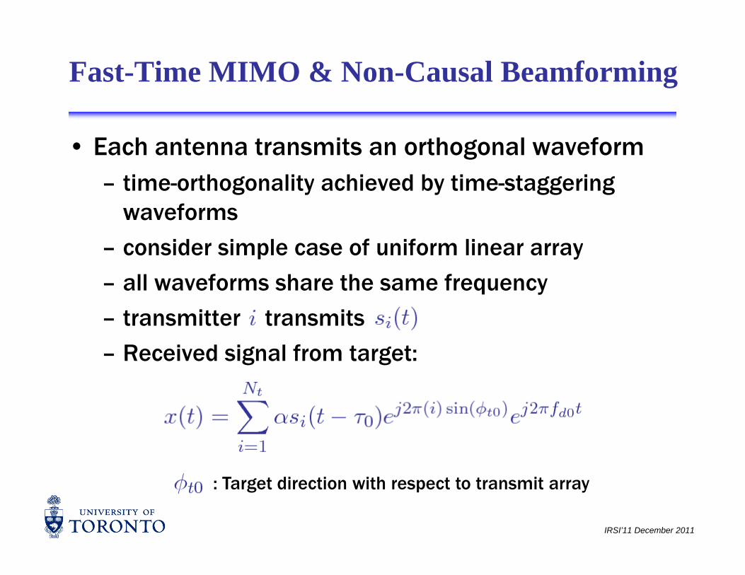
Fast-Time MIMO & Non-Causal Beamforming
• Each antenna transmits an orthogonal waveformtime orthogonality achieved by time staggering – time-orthogonality achieved by time-staggering waveforms
– consider simple case of uniform linear arrayconsider simple case of uniform linear array
– all waveforms share the same frequency
– transmitter transmitstransmitter transmits
– Received signal from target:
IRSI’11 December 2011
: Target direction with respect to transmit array
Non-Causal Beamforming (2)
• Similar expression for clutter and other forms of interferenceinterference
• Key: on matched filtering, each waveform separates separates – in addition, there are pulses in a CPI
– resulting in a vector of the formresulting in a vector of the form
– : space-time steering vector : space time steering vector •the spatial component comes from the angle with
respect to the transmitter
IRSI’11 December 2011
– : the noise and interference vector
Non-Causal Beamforming (3)
• This is the exact same model as we had for STAP!• This is the exact same model as we had for STAP!– this is adaptive processing at a single receive
antenna using the transmitted waveforms g
– can use all of what we know about STAP
– rather dramatically called non-causal beamformingy g•though the beamforming “happens” after the
transmission, not before
– if multiple receive elements, size of problem increases, no conceptual change
has been applied to the Jindalee OTHR in Australia
IRSI’11 December 2011
– has been applied to the Jindalee OTHR in Australia (see Frazer, Abramovich and Johnson, Radar 2008)

Slow-Time MIMO
• All transmitters transmit at the same time and use the same waveformthe same waveform– however, sub-divide the Doppler space into
regionsregions
– can be achieved by using an effective PRF that is reduced by a factor of :
– signal transmitted from element
IRSI’11 December 2011
Slow-Time MIMO (2)
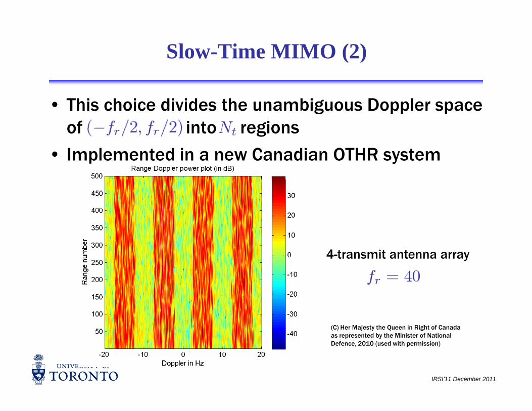
• This choice divides the unambiguous Doppler space of into regionsof into regions
• Implemented in a new Canadian OTHR system
4-transmit antenna array
(C) Her Majesty the Queen in Right of Canada as represented by the Minister of National
IRSI’11 December 2011
as represented by the Minister of National Defence, 2010 (used with permission)
Slow-Time MIMO (3)
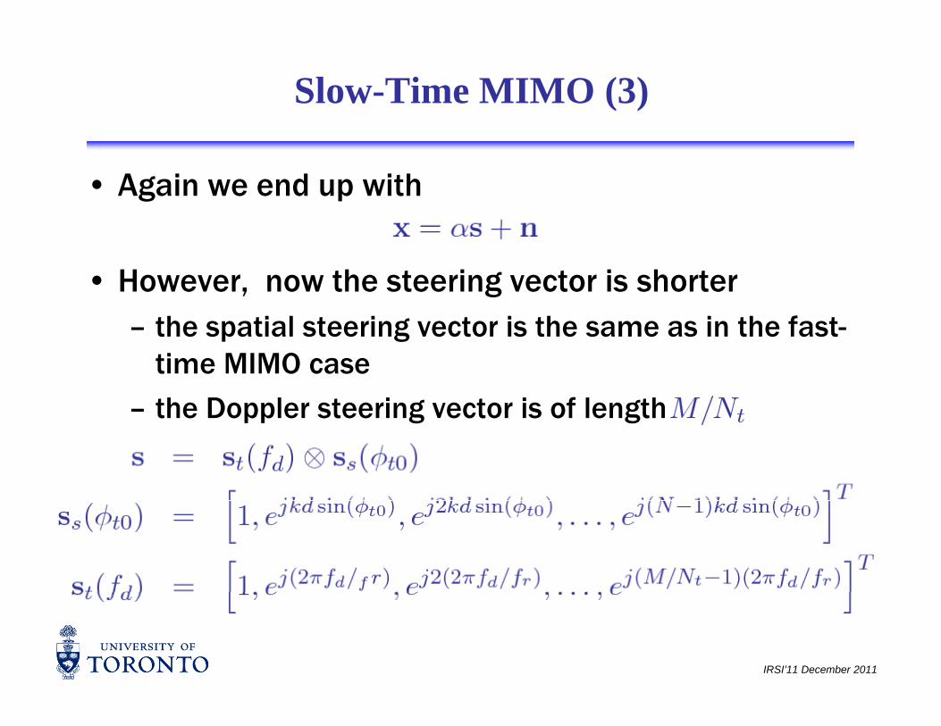
• Again we end up with
• However, now the steering vector is shorterth ti l t i t i th i th f t– the spatial steering vector is the same as in the fast-time MIMO case
– the Doppler steering vector is of length – the Doppler steering vector is of length
IRSI’11 December 2011
Slow-Time MIMO (3)
• The problem size (with a single receive antenna) is thereforetherefore– temporal degrees of freedom
– spatial degrees of freedom– spatial degrees of freedom
• Again, one can apply one’s favourite STAP algorithm as desiredalgorithm as desired– note that the orthogonality here is in the Doppler
domain
IRSI’11 December 2011
References Used/Further Reading
• “Principles of Modern Radar”, M. A. Richards, J.A. Scheer, W.A. Holm (eds.), SciTech Publishers, 2010
• “Radar Signals” N Levanon and E Mozeson John Wiley & Sons 2004• Radar Signals , N. Levanon and E. Mozeson, John Wiley & Sons, 2004
• “Waveform Diversity: Theory and Applications”, U. Pillai, K. Y. Li, I. Selesnick, B. Himed, McGraw Hill, 2011
• “MIMO Radar Signal Processing”, J. Li and P. Stoica (eds.), John Wiley, 2008
• “Principles of Waveform Diversity and Design”, M. Wicks, E. Mokole, S. Blunt, R. Schneibleand V. Amuso (eds.), SciTech Publishers, 2010
• “Fundamentals of Multisite Radar Systems”, V.S. Chernyak, Gordon and Breach Science Publishers, 1998 (translated from Russian).Publishers, 1998 (translated from Russian).
• M.R. Bell, “Information theory and radar waveform design “, IEEE Trans on Information Theory, vol. 39, no. 5, Sept. 1993.
• J. Ward, “Space-time adaptive processing for airborne radar,” MIT Lincoln Laboratory, T h i l R t F19628 95 C 0002 D b 1994Technical Report, F19628-95-C-0002, December 1994.
• R. Daher and R.S. Adve, “A notion of diversity order in distributed radar networks”, Accepted for publication, IEEE Trans. on Aerospace and Electronic Systems. Available at http://www.comm.utoronto.ca/~rsadve/Publications/Rani_DiversityOrderJournal.pdf
IRSI’11 December 2011
References Used/Further Reading
• B. Jung, R.S. Adve, J. Chun, and M.C. Wicks, “Detection using frequency diversity with distributed sensors”, Accepted for publication, IEEE Trans. on Aerospace and Electronic Systems. Available at Systems. Available at http://www.comm.utoronto.ca/~rsadve/Publications/Jung_FreqDivJournal.pdf
• P. Varshney, Distributed Detection and Data Fusion. Springer-Verlag, 1996.
• J. N. Tsitsiklis, “Decentralized detection,” Advances in Statistical Signal Processing, Signal D t ti l 2 297 344 1993Detection, vol. 2, pp. 297-344, 1993.
• S. Thomopoulos, R. Viswanathan, and D. Bougoulias, “Optimal distributed decision fusion,” IEEE Trans. on Aerospace and Electronic Systems., vol. 25, pp. 761-765, September 1989.
• R. Tenney and N. Sandels, “Detection with distributed sensors,” IEEE Trans. on Aerospace and Electronic Systems, vol. 17, no. 4, 1981.
• Y. Abramovich and G. Frazer, “Bounds on the volume and height distributions for the MIMO radar ambiguity function”, IEEE Signal Processing Letters, vol. 15, pp. 505-508, 2008
• G San Antonio D Fuhrmann and F Robey “MIMO radar ambiguity functions” IEEE • G. San Antonio, D. Fuhrmann and F. Robey, MIMO radar ambiguity functions , IEEE Journal on Selected Areas in Signal Processing, vol. 1, no. 1., pp. 167-177, Jan. 2007
• B. Friedlander, “Waveform design for MIMO radar”, IEEE Transactions on Aerospace and Electronic Systems, vol. 43, no. 3, pp. 1227-1238, March 2007
IRSI’11 December 2011
• Y. Yang and R.S. Blum, “MIMO radar waveform design based on mutual information and minimum mean-square error estimation”, IEEE AES, vol. 43, no. 1, pp. 330-343, Jan 2007
References Used/Further Reading
• G. J. Frazer, Y. I. Abramovich, and B. A. Johnson, “Use of adaptive non-causal transmit beamforming in OTHR: Experimental results,” in Proceedings of the 2008 International Radar Conference, May 2008.Radar Conference, May 2008.
• V. Mecca, J. L. Krolik, and F. C. Robey, “Beamspace slow-time MIMO radar for multi- path clutter mitigation,” in Proceedings of the 2008 IEEE International Conference on Acoustics, Speech and Signal Processing, pp. 2313–2316, April 2008.
also Chap 7 of “MIMO Radar Signal Processing” J Li and P Stoica (eds ) John Wiley 2008– also Chap 7 of “MIMO Radar Signal Processing”, J. Li and P. Stoica (eds.), John Wiley, 2008
• R.J. Riddolls, “Joint transmit-receive adaptive beamforming experimental results from an auroral-zone Canadian over-the-horizon radar system”, Proceedings of the 2011 IEEE Radar Conference, May 2011.
• R. J. Riddolls, M. Ravan and R.S. Adve, “Canadian HF Over-the-Horizon Radar experiments using MIMO techniques to control auroral clutter”, Proceedings of the 2010 IEEE Radar Conference, May 2010.
IRSI’11 December 2011


![Hard Decision-Based PWM for MIMO-OFDM Radar · 2. MIMO-OFDM Radar Signal Model-Based PWM 2.1. MIMO-OFDM Radar Systems Structure In [1], OFDM technique has the advantage of combating](https://static.fdocuments.us/doc/165x107/5e6a685a5002aa073940e3bf/hard-decision-based-pwm-for-mimo-ofdm-radar-2-mimo-ofdm-radar-signal-model-based.jpg)

