2-1

CHAPTER 2

WAVE THEORIES

2.1 Basic Hydrodynamic Equations

Continuity Equation

Application of the principle of conservation of mass to the flow into and outside

an element of fluid leads to the following equation of continuity (Streeter and Wylie,

1986).

0=∂

∂+

∂

∂+

∂

∂

z

w

y

v

x

u 2.1

where u, v, w are three components of the fluid velocity at a point along the co-

ordinate axes of x, y and z respectively.

Rotational Flow:

With the passage of time an element of fluid may undergo a rotation. The

rotations of a fluid element about the x, y and z axes respectively are given by, (See Fig

2.1 for a simple 2-D case)

∂

∂−

∂

∂=

y

w

z

vx

2

1ω 2.2

∂

∂−

∂

∂=

z

u

x

wy

2

1ω 2.3

∂

∂−

∂

∂=

x

v

y

uz

2

1ω 2.4

Irrotational Flow:

Many complex fluid problems become tractable if we assume that the net rotation

of the fluid element about any of the x, y and z axes is zero, i.e.

0=== zyx ωωω 2.5

Such a flow is called Irrotational Flow.

2-2

Since rotation can be produced by the moment of shear forces acting tangential on

the fluid element, inviscid or frictionless fluid (implying absence of shear forces) would

make the flow irrotational. Wave motion is normally assumed to involve negligible

viscosity and internal friction.

Velocity potential

In accordance with preceding Equation (2.5), for an irrotational flow,

0=== zyx ωωω

Typically then,

∴

∂

∂−

∂

∂=

z

u

x

wy

2

1ω = 0 (from equation (2.3))

∴z

u

x

w

∂

∂=

∂

∂ 2.6

If we define a scalar function ‘φ ’ of position x, y, z and time 't' having continuous

derivative, i.e

xzzx ∂∂

∂=

∂∂

∂ φφ 22

2.7

or,

∂

∂

∂

∂=

∂

∂

∂

∂

xzzx

φφ, 2.8

then comparing with equation (2.6) we get

xu

zw

∂

∂=

∂

∂=

φφ; 2.9

Similarly it can be shown, from other rotation equations, that

yv

∂

∂=

φ 2.10

The assumption of flow irrotationality thus leads to the establishment of the

velocity potential ‘φ ’. Putting u, v and w by equations (2.9) and (2.10), into the

continuity equation (2.1), we get

2-3

02

2

2

2

2

2

=∂

∂+

∂

∂+

∂

∂

zyx

φφφ 2.11

i.e. 02 =∇ φ

This is called the Laplace form of continuity equation.

Stream Function

For any 2-D flow a function ),( yxψ can be defined such that its partial derivative

along any direction would give the flow velocity along the clockwise normal orientation,

i.e.

uy

vx

=∂

∂−=

∂

∂ ψψ; 2.12

This function ψ is called the stream function.

Bernoulli Equation

Based on the Newton's equation for motion of rigid bodies, viz, force = mass x

acceleration. Euler equations of motion for fluid flow can be derived assuming the

absence of shear forces. These equations, when integrated, lead us to the dynamic

equation of Bernoulli:

( )0

2

222

=∂

∂+++

++

tgz

pwvu φ

ρ 2.13

where u, v and w are the three components of fluid velocity at a point, φ is the

velocity potential, t is the time, p is the pressure acting at the point, ρ is the mass density

of the fluid, g is the acceleration due to gravity and z is the elevation of the point.

2.2 Wave Theories

Wave theories yield the information on wave motion like water particles

kinematics and wave speed, using the input information of wave height, its period and

depth of water at the site. There are more than a dozen different theories available in this

regard. However, only a few of them that are more common used and these are described

below: All wave theories involve some common assumptions, viz,

2-4

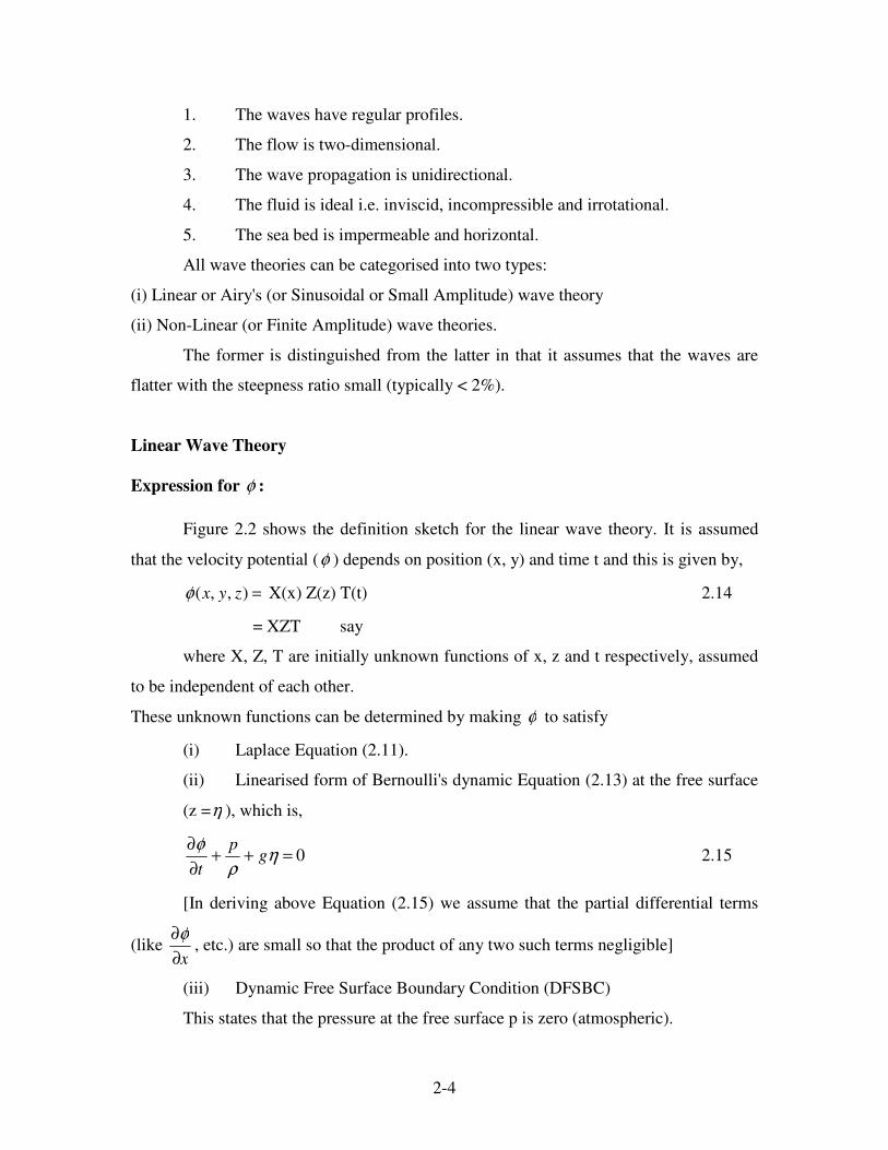
1. The waves have regular profiles.

2. The flow is two-dimensional.

3. The wave propagation is unidirectional.

4. The fluid is ideal i.e. inviscid, incompressible and irrotational.

5. The sea bed is impermeable and horizontal.

All wave theories can be categorised into two types:

(i) Linear or Airy's (or Sinusoidal or Small Amplitude) wave theory

(ii) Non-Linear (or Finite Amplitude) wave theories.

The former is distinguished from the latter in that it assumes that the waves are

flatter with the steepness ratio small (typically < 2%).

Linear Wave Theory

Expression for φ :

Figure 2.2 shows the definition sketch for the linear wave theory. It is assumed

that the velocity potential (φ ) depends on position (x, y) and time t and this is given by,

=),,( zyxφ X(x) Z(z) T(t) 2.14

= XZT say

where X, Z, T are initially unknown functions of x, z and t respectively, assumed

to be independent of each other.

These unknown functions can be determined by making φ to satisfy

(i) Laplace Equation (2.11).

(ii) Linearised form of Bernoulli's dynamic Equation (2.13) at the free surface

(z =η ), which is,

0=++∂

∂η

ρ

φg

p

t 2.15

[In deriving above Equation (2.15) we assume that the partial differential terms

(like x∂

∂φ, etc.) are small so that the product of any two such terms negligible]

(iii) Dynamic Free Surface Boundary Condition (DFSBC)

This states that the pressure at the free surface p is zero (atmospheric).

2-5

(iv) Kinematic Free Surface Boundary Condition (KFSBC)

It ensures that the free surface is continuous.

(v) Bottom Boundary Condition (BBC)

This means that the velocity normal to the sea bottom is zero.

The expression for φ determined in this way (Ippen 1965) is

)sin()cosh(2

))(cosh(tkx

kd

zdkgHω

ωφ −

+= 2.16

where

H = wave height

ω = Circular wave frequency = T

π2

T = Wave period

k = Wave number = L

π2

L = Wave length

z = Vertical co-ordinate of the point at which φ is being

considered (from the

SWL)

d = Water depth

x = Horizontal co-ordinate of the point (w.r.t any arbitrary origin

at SWL)

t = Time instant.

Expression for wave profile:

Starting with ‘φ ’ as above and applying the DFSBC, the sea surface elevation

(η ), at given x and t is

)cos(2

tkxH

ωη −= 2.17

2-6

Expression for wave Celerity:

If we move with the same speed as that of the wave, the wave form (η ) will

appear stationary, i.e., from equation (2.17)

kx-ω t = constant

∴ wave speed or celerity

C = T

L

kdt

dx==−

ω 2.18

Combining KFSBC and DFSBC we get linear relationship:

ω 2 = gk tanh (kd) 2.19

which is useful to obtain 'k' from the wave frequency (ω ). Substituting C = ω /k

in this equation, we get

)tanh(2

kdgT

Cπ

= 2.20

Simplification in shallow and deep water:

In shallow water (d<L/20) and deep water (d>L/2) cosh, sinh and tanh terms

involved in the above equations take limiting values:

for small 'kd': sinh (kd) ≈ kd; cosh (kd) ≈ 1;tanh (kd) ≈ kd 2.21

for large 'kd': sinh (kd) ≈ cosh (kd)2

kde

≈ : tanh (kd) ≈ 1 2.22

Hence the above equations (2.16) to (2.20) can be simplified. In deep water from

equations (2.20) and (2.22), the deep water wave celerity,C0 is

π20

gTC = 2.23

If L0 is the wavelength in deep water, C0 = L0/T gives,

π2

2

0

gTL = 2.24

Similarly in shallow water, Equation (2.20) after a little modification becomes

gdC s = 2.25

where Cs = wave speed in shallow water

2-7

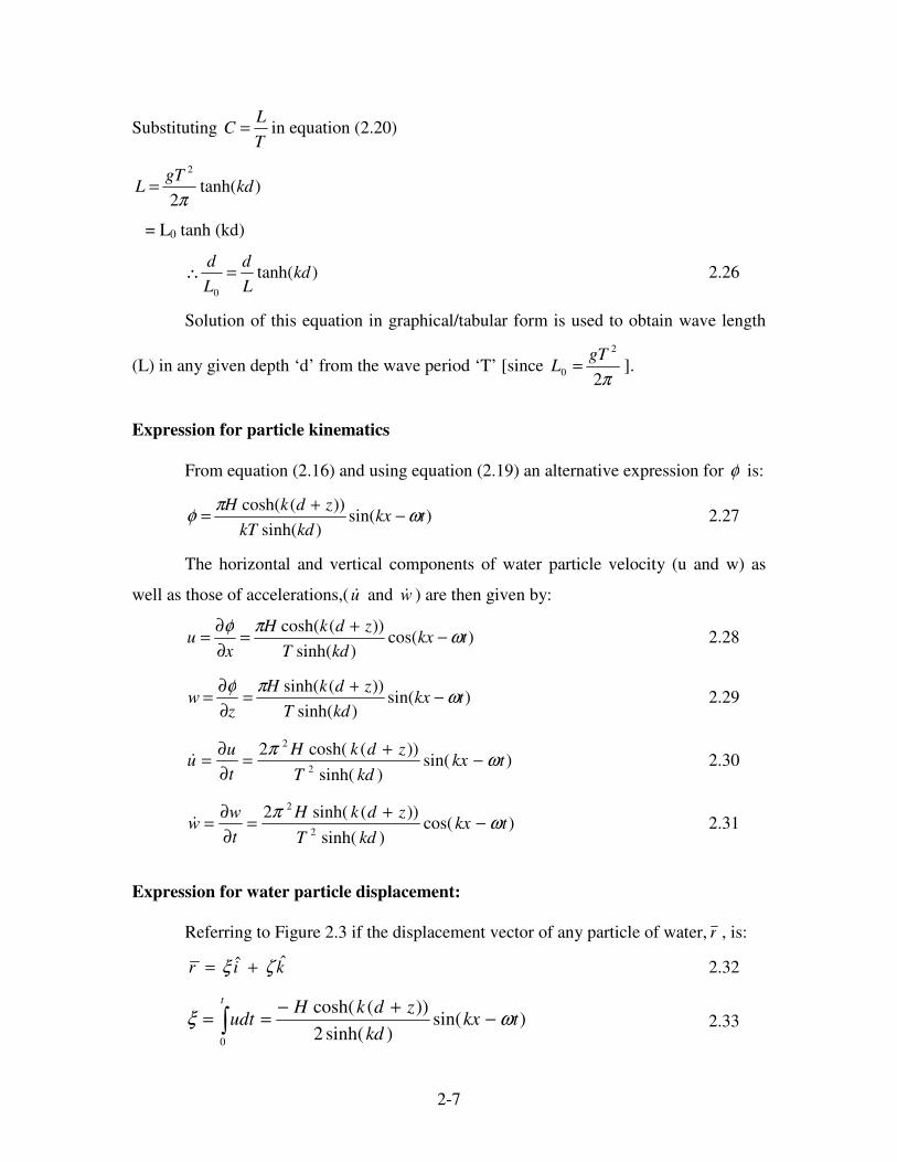
Substituting T

LC = in equation (2.20)

)tanh(2

2

kdgT

Lπ

=

= L0 tanh (kd)

)tanh(0

kdL

d

L

d=∴ 2.26

Solution of this equation in graphical/tabular form is used to obtain wave length

(L) in any given depth ‘d’ from the wave period ‘T’ [since π2

2

0

gTL = ].

Expression for particle kinematics

From equation (2.16) and using equation (2.19) an alternative expression for φ is:

)sin()sinh(

))(cosh(tkx

kdkT

zdkHω

πφ −

+= 2.27

The horizontal and vertical components of water particle velocity (u and w) as

well as those of accelerations,(u& and w& ) are then given by:

)cos()sinh(

))(cosh(tkx

kdT

zdkH

xu ω

πφ−

+=

∂

∂= 2.28

)sin()sinh(

))(sinh(tkx

kdT

zdkH

zw ω

πφ−

+=

∂

∂= 2.29

)sin()sinh(

))(cosh(22

2

tkxkdT

zdkH

t

uu ω

π−

+=

∂

∂=& 2.30

)cos()sinh(

))(sinh(22

2

tkxkdT

zdkH

t

ww ω

π−

+=

∂

∂=& 2.31

Expression for water particle displacement:

Referring to Figure 2.3 if the displacement vector of any particle of water, r , is:

kir ˆˆ ζξ += 2.32

)sin()sinh(2

))(cosh(

0

tkxkd

zdkHudt

t

ωξ −+−

== ∫ 2.33

2-8

)cos()sinh(2

))(sinh(

0

tkxkd

zdkHwdt

t

ωξ −+−

== ∫

From equations (2.28) and (2.29) respectively,

If a1 = )sinh(2

))(cosh(

kd

zdkH + and b1 =

)sinh(2

))(sinh(

kd

zdkH +

)sin(1 tkxa ωξ −−=

)cos(1 tkxb ωζ −=

squaring and adding,

12

1

2

2

1

2

=+ba

ζξ 2.34

This shows that the locus of wave particles is an ellipse in any general water

depth as shown in Figure 2.3.

In deep water, using equation (2.22)

kze

Hba

211 =

This indicates that the water particles trace out a circle. Further, at free surface,

z=0. Hence,

211

Hba ==∴

at z = - 2

L, He

Hba

L

L 02.02

2

2

11 ===

−

π

which is a negligible quantity.

In shallow water, using equation (2.21)

kd

Ha

21 = (independent of z)

d

zdHb

2

)(1

+=

= 2

H at z = 0

= 0 at z = - d

The paths followed by water particles in different depths are therefore as shown in

Figure 2.3.

2-9

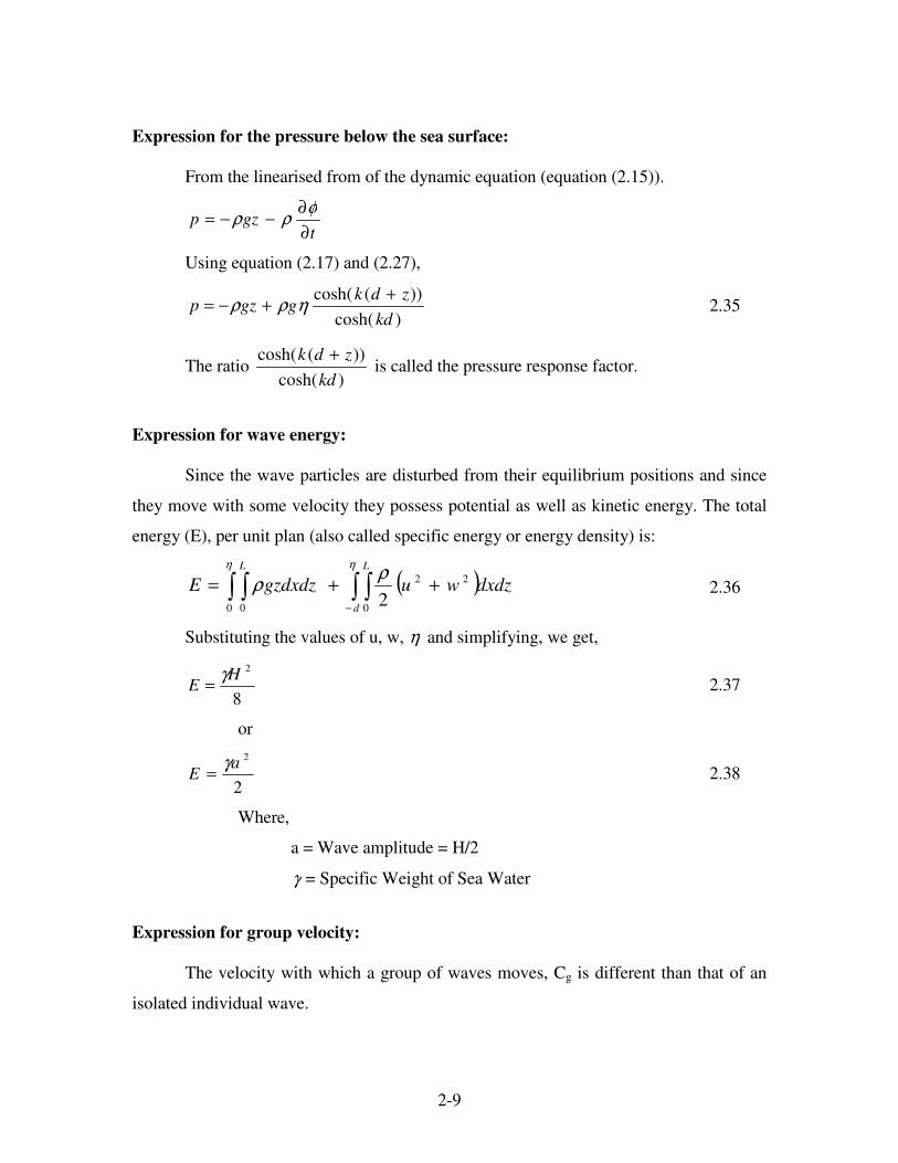
Expression for the pressure below the sea surface:

From the linearised from of the dynamic equation (equation (2.15)).

tgzp

∂

∂−−=

φρρ

Using equation (2.17) and (2.27),

)cosh(

))(cosh(

kd

zdkggzp

++−= ηρρ 2.35

The ratio )cosh(

))(cosh(

kd

zdk + is called the pressure response factor.

Expression for wave energy:

Since the wave particles are disturbed from their equilibrium positions and since

they move with some velocity they possess potential as well as kinetic energy. The total

energy (E), per unit plan (also called specific energy or energy density) is:

( )∫ ∫ ∫ ∫−

++=η η

ρρ

0 0 0

22

2

L

d

L

dxdzwugzdxdzE 2.36

Substituting the values of u, w, η and simplifying, we get,

8

2H

Eγ

= 2.37

or

2

2a

Eγ

= 2.38

Where,

a = Wave amplitude = H/2

γ = Specific Weight of Sea Water

Expression for group velocity:

The velocity with which a group of waves moves, Cg is different than that of an

isolated individual wave.

2-10

dk

d

kC

kg

ωω=

∆

∆=

→∆ 0lim 2.39

Using the linear dispersion equation (2.19), above equation reduces to

Cg = nC 2.40

where,

n = f(kd) =

+

)2sinh(

21

2

1

kd

kd 2.41

With the help of shallow and deep water approximations, Equations (2.21) and

(2.22) respectively, it is easy to see that in deep water and in shallow water

2

0

0

CC g = 2.42

and in shallow water

Cg = Cs = gd 2.43

Expression for wave power or energy flux:

This is defined as the average rate of transmission of wave energy per unit lateral

width along the direction of the wave propagation.

( )∫ ∫−

+++=∴

ηρ

ρd

T

dzdtuwugzpT

P0

22

2

1 2.44

Substituting the value of η , p, u and w from the previous expressions,

ECnCET

LHgnP g===

8

2

ρ 2.45

Finite Amplitude Wave Theories

General Method of Solution:

In preceding small amplitude wave theory the wave steepness (H/L) was assumed

to be small (so that its higher powers became negligible) and the expressions for φ and η

turned out to be

)0sin(1C=φ 2.46

and

2-11

)cos( θη a= 2.47

where,

C1 = f (H, T, d) (see equation (2.27))

( )tkx ωθ −= , phase angle

a = H/2

When wave steepness value is high, or finite, above assumption becomes no

longer valid and a different solution for φ results. As per different alternative methods to

formulate ‘φ ’ we have different theories like Stokes, Cnoidal, Solitary, Dean’s, etc.under

the Finite Amplitude category. A general common procedure to obtain the wave

properties, in these theories, is as discussed below:

First, the φ (or ψ ) is formulated as some unknown function of given H, T, d

values containing unknown coefficients. This φ (or ψ ) is then made to satisfy the

continuity equation, dynamic equation, irrotationality equation and various boundary

conditions discussed in the previous section. By solving all such equations

simultaneously the unknown coefficients are established and φ (or ψ ) in turn is

obtained. Once φ (or ψ ) is known its derivatives like φ,,,, wwuu && etc. automatically

follow.

Stokes Wave Theory:

The φ and η are modelled in Stokes theory using perturbation parameters b and a

respectively as below:

)sin(),,(1

θφφ ndTHb n

M

n

n∑=

= 2.48

)cos(),,(1

θη ndTHfa n

M

n

n∑=

= 2.49

where bn and an are initially unknown functions of H, T, d and so also φ n

and fn.

2-12

The above represented series can be explained to any order (considering powers

of (H/L) only upto that order) to obtain the Stokes theory of the corresponding order. e.g.

in the Stokes second order theory,

)2sin()sin( 21 θθφ bb +=

)2cos()cos( 21 θθη aa +=

where, (b1,b2,a1,a2 are functions of H, T and d)

The fifth order theory is popular owing to its better prediction of the actual water

particle kinematics.

The procedure followed in the fifth order theory to arrive at the values of particle

kinematics is as below:

1. From the given values of H, T, d obtain the unknowns λ and kd by the two

expressions given below that result from the application of KFSBC and FSBCs.

[ ]d

HBBB

kd 2)(

1 5

5535

2

33 =+++ λλλ 2.50

kd tanh (kd) [ ]2

24

2

2

1 41gT

dCC πλλ =++ 2.51

where Bij,Ci (for various values of i and j) are initially unknown functions of kd as

listed in Appendix 3.1, which also explains additional symbol Aij used below:

2. Obtain φ using,

∑=

+′=5

1

)sin())(cosh(n

n nzdnkk

Cθφφ 2.52

where,

15

5

13

3

111 AAA λλλφ ++=′

24

4

22

2

2 AA λλφ +=′

35

5

33

3

3 AA λλφ +=′

44

4

4 Aλφ =′

55

5

5 Aλφ =′

[ ]4

2

2

11)tanh( λλ CCkdk

gc ++=

2-13

3. ∑=

+′=5

1

)cos())(cosh(n

n nzdnkncu θφ 2.53

∑=

+′=5

1

)sin())(sinh(n

n nzdnkncw θφ 2.54

∑=

+′=5

1

2 )sin())(cosh(n

n nzdnkncu θφω& 2.55

∑=

+′−=5

1

2 )cos())(sinh(n

n nzdnkncw θφω& 2.56

4. ∑=

′=5

1

)cos(1

n

n nk

θηη 2.57

where,

λη =′1

24

4

22

2

2 BB λλη +=′

35

5

33

3

3 BB λλη +=′

44

4

4 Bλη =′

55

5

5 Bλη =′

A computer program carrying out all above steps can be easily developed

[Chaudhari (1985), Kankarej (1992)].

Cnoidal Theory:

The general definitions of Cnoidal theory are given in the Figure 2.4.This theory

involves formulating φ in terms of the elliptic cosine or Cnoidal function:

( ) )(cos xfSDgdL

σφ

=′

2.58

= )(...............!4!2

14

422

2xf

DS

DS

++− σσ 2.59

where,

2-14

1'''',

,<<

=

z

directionxhorizontalthelongaLlengthtypicalchosena

dWaterDepthσ

(very small)

d

zdS

+= [z = vertical co-ordinate from the sea bed; positive upwards.(Figure

2.4)]

dx

dD = ;

L

CtxX

′

−=

Solution φ of involves elliptic functions, typically the complete Elliptic integral

of first kind, K (k), where k is the argument depending upon H, T, d and ranging from 0

to 1.The application of them to obtain water particle kinematics involves elaborate

computer programming. However, for certain application, like determination of wave

profile and wave length, graphical solutions are available (Wiegel (1965).

Solitary Wave Theory:

When the value of the argument k of K (k) tends to its upper limit 1,K (k)

approaches sech (k) and a great simplification in the resulting values emerges. The

resulting theory is called the solitary wave theory.(See Figure 2.5 for the definition

sketch).Solitary theory of second order is found to be simple and satisfactory for steep

waves in shallow water.(See Sarpkaya and Issacson,(1981)).

Dean Stream Function Theory:

Herein, in contrast to previous theories a solution for stream function ψ is sought

for as expressed below:

A reference frame advancing with the same speed is taken so that the flow

becomes steady and the steady state Bernoulli's equation becomes applicable. (See Figure

2.6)

∑=

++−=

M

n

nL

xnzd

LnXCz

1

2cos)(

2sinh

ππψ 2.60

with M representing the desired order of expression.

2-15

Xn are the coefficients that are obtained by following a numerical procedure. The

resulting computer program is complicated. But tabular aids are available (SPM (1984)).

Trochoidal Wave Theory:

In this wave theory, the wave profile is idealized to that of a trochoid which is a

curve generated by the locus of any point on a circle as the circle is imagined to be

translating along a horizontal line.

If (x0,z0) are the co-ordinates of the mean position of a water particle then its

trajectories at any time are given by,

)sin()exp()2/( 000 tkxkzHxx ω−+=

)cos()exp()2/( 000 tkxkzHzz ω−+=

These quantities can be further differentiated to yield the velocity components as

txu ∂∂= and tzw ∂∂= .

Method of Complex variables:

Another technique of getting the wave parameters involves transforming the

physical region of the fluid bounded by the ocean bottom and the free surface wave

profile into an annulus region bounded by an outer circle of unit radius representing the

free surface and an inner circle corresponding to the ocean bottom. The flow in this

annulus complex plane is potential clockwise vortex whose properties are known and can

therefore be mapped on the complex plane of φ and ψ plane. The mapping of the

physical plane and the φ -ψ plane can as well be done using a perturbation parameter

technique.

Non-linear versus Linear Theory

The profile of a linear wave is symmetrical with respect to the undisturbed or the

still water level (SWL) whereas in case of a typical non-linear wave height of the crest is

greater than the depth of the through as shown in Figure 2.7.

As the order of a non-linear theory increases, the crests become more and more

steep and the troughs become more and more flat.

2-16

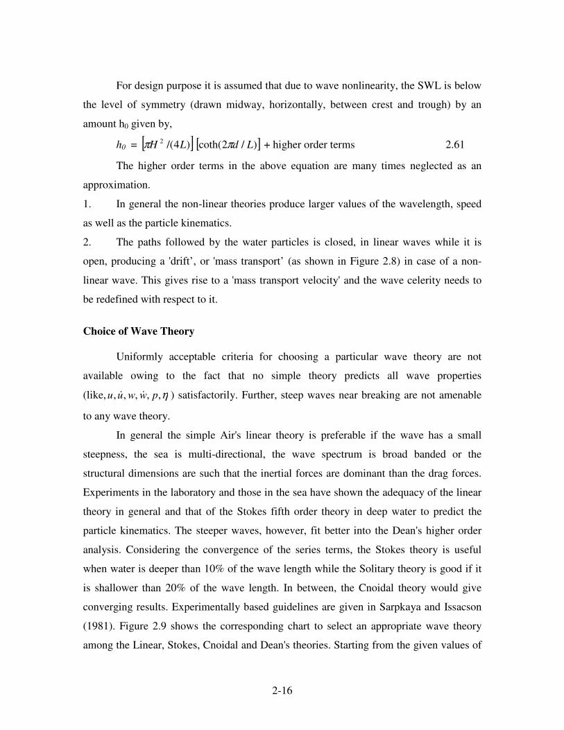
For design purpose it is assumed that due to wave nonlinearity, the SWL is below

the level of symmetry (drawn midway, horizontally, between crest and trough) by an

amount h0 given by,

h0 = [ ] [ ])/2coth()4/(2 LdLH ππ + higher order terms 2.61

The higher order terms in the above equation are many times neglected as an

approximation.

1. In general the non-linear theories produce larger values of the wavelength, speed

as well as the particle kinematics.

2. The paths followed by the water particles is closed, in linear waves while it is

open, producing a 'drift’, or 'mass transport’ (as shown in Figure 2.8) in case of a non-

linear wave. This gives rise to a 'mass transport velocity' and the wave celerity needs to

be redefined with respect to it.

Choice of Wave Theory

Uniformly acceptable criteria for choosing a particular wave theory are not

available owing to the fact that no simple theory predicts all wave properties

(like, η,,,,, pwwuu && ) satisfactorily. Further, steep waves near breaking are not amenable

to any wave theory.

In general the simple Air's linear theory is preferable if the wave has a small

steepness, the sea is multi-directional, the wave spectrum is broad banded or the

structural dimensions are such that the inertial forces are dominant than the drag forces.

Experiments in the laboratory and those in the sea have shown the adequacy of the linear

theory in general and that of the Stokes fifth order theory in deep water to predict the

particle kinematics. The steeper waves, however, fit better into the Dean's higher order

analysis. Considering the convergence of the series terms, the Stokes theory is useful

when water is deeper than 10% of the wave length while the Solitary theory is good if it

is shallower than 20% of the wave length. In between, the Cnoidal theory would give

converging results. Experimentally based guidelines are given in Sarpkaya and Issacson

(1981). Figure 2.9 shows the corresponding chart to select an appropriate wave theory

among the Linear, Stokes, Cnoidal and Dean's theories. Starting from the given values of

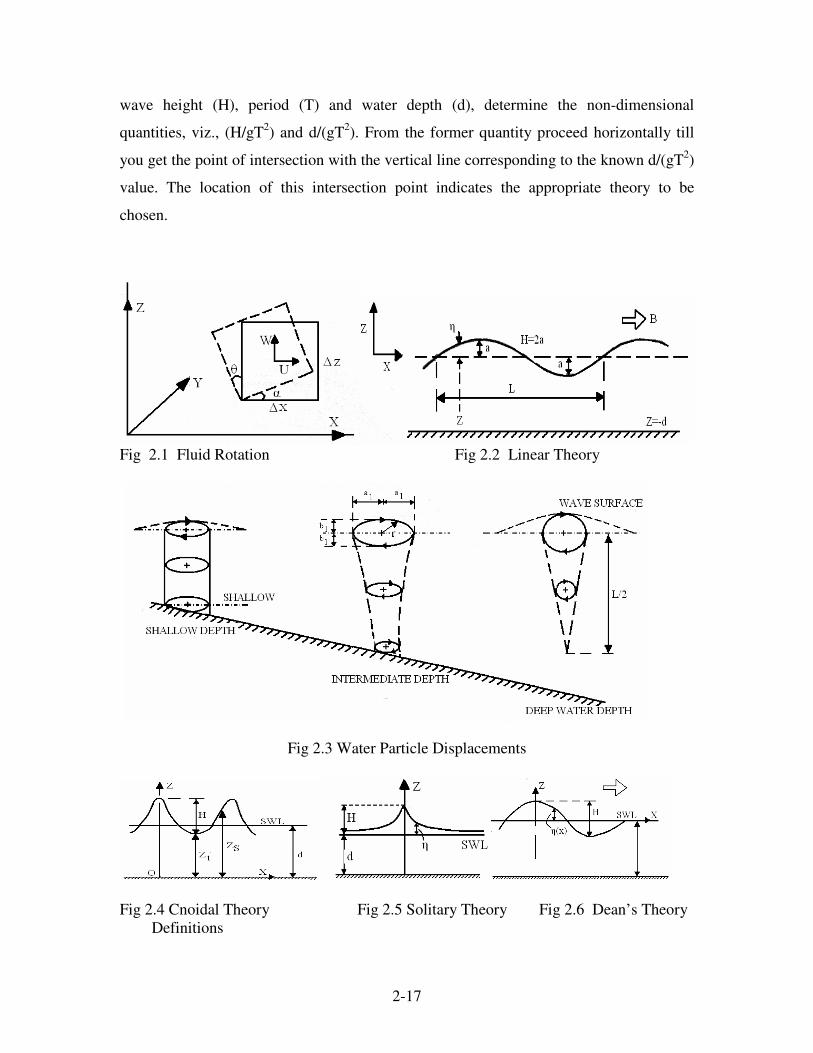
2-17

wave height (H), period (T) and water depth (d), determine the non-dimensional

quantities, viz., (H/gT2) and d/(gT

2). From the former quantity proceed horizontally till

you get the point of intersection with the vertical line corresponding to the known d/(gT2)

value. The location of this intersection point indicates the appropriate theory to be

chosen.

Fig 2.1 Fluid Rotation Fig 2.2 Linear Theory

Fig 2.3 Water Particle Displacements

Fig 2.4 Cnoidal Theory Fig 2.5 Solitary Theory Fig 2.6 Dean’s Theory

Definitions

2-18

Linear Non Linear Solitary

Fig 2.7 Comparison of Wave Profiles

Fig 2.8 Closed and Open Orbits

2-19

Fig 2.9 Choice of a Wave Theory (Ref. Sarpakaya and Issacson, 1981)