Wave-Maintained Annular Modes of Climate Variability

4414 VOLUME 13J O U R N A L O F C L I M A T E

q 2000 American Meteorological Society

Wave-Maintained Annular Modes of Climate Variability*

VARAVUT LIMPASUVAN AND DENNIS L. HARTMANN

Department of Atmospheric Sciences, University of Washington, Seattle, Washington

(Manuscript received 15 July 1999, in final form 19 January 2000)

ABSTRACT

The leading modes of month-to-month variability in the Northern and Southern Hemispheres are examinedby comparing a 100-yr run of the Geophysical Fluid Dynamics Laboratory GCM with the NCEP–NCAR re-analyses of observations. The model simulation is a control experiment in which the SSTs are fixed to theclimatological annual cycle without any interannual variability. The leading modes contain a strong zonallysymmetric or annular component that describes an expansion and contraction of the polar vortex as the midlatitudejet shifts equatorward and poleward. This fluctuation is strongest during the winter months. The structure andamplitude of the simulated modes are very similar to those derived from observations, indicating that thesemodes arise from the internal dynamics of the atmosphere.

Dynamical diagnosis of both observations and model simulation indicates that variations in the zonally sym-metric flow associated with the annular modes are forced by eddy fluxes in the free troposphere, while theCoriolis acceleration associated with the mean meridional circulation maintains the surface wind anomaliesagainst friction. High-frequency transients contribute most to the total eddy forcing in the Southern Hemisphere.In the Northern Hemisphere, stationary waves provide most of the eddy momentum fluxes, although high-frequency transients also make an important contribution. The behavior of the stationary waves can be partlyexplained with index of refraction arguments. When the tropospheric westerlies are displaced poleward, Rossbywaves are refracted equatorward, inducing poleward momentum fluxes and reinforcing the high-latitude west-erlies. Planetary Rossby wave refraction can also explain why the stratospheric polar vortex is stronger whenthe tropospheric westerlies are displaced poleward. When planetary wave activity is refracted equatorward, itis less likely to propagate into the stratosphere and disturb the polar vortex.

1. Introduction

Recent observations demonstrate that month-to-month tropospheric variation in the Northern Hemi-sphere is dominated by a mode that has a strong zonallysymmetric or annular component (Baldwin and Dunk-erton 1999; Thompson and Wallace 1998, 2000, here-after TW). The zonal mean part of the Northern Hemi-sphere variability is remarkably similar to that of theannular atmospheric variability in the Southern Hemi-sphere (e.g., Trenberth 1984; Yoden et al. 1987; Kidson1988; Shiotani 1990; Nigam 1990; Karoly 1990; Hart-mann and Lo 1998). In particular, despite contrastingland–sea distribution, the zonally symmetric componentof the Northern and Southern Hemisphere annularmodes (hereafter NAM and SAM, respectively) de-

* Joint Institute for the Study of the Atmosphere and Ocean Con-tribution Number 703.

Corresponding author address: Varavut Limpasuvan, Departmentof Chemistry and Physics, Coastal Carolina University, P.O. Box261954, Conway, SC 29528.E-mail: [email protected]

scribes a north–south movement of the midlatitude zonaljet in which the anomalous structure exhibits a dipolepattern in westerly winds with centers at high (508–608)and low (308–408) latitudes. By convention, the index(i.e., time series) of the annular mode is positive(‘‘high’’ phase) when the zonal jet is displaced polewardfrom its climatological position. During the low phase,the jet shifts equatorward. The polar vortex expands andcontracts in relation to the varying jet position.

In the Southern Hemisphere (SH), the annular modeof variability is associated with the low-frequency zonalmean zonal wind (u) vacillation between 408 and 608S.This fluctuation is relatively easy to simulate in atmo-spheric models and has been shown to result from theinteraction between transient eddies and zonal meanflow (e.g., Robinson 1991; Yu and Hartmann 1993).Since stationary wave features are weak in the SH, theeddy interaction with the zonal flow is contributed al-most entirely by transient waves resulting from the in-stability of the zonal mean flow. Hartmann (1995) andHartmann and Lo (1998) observe that synoptic wavestructures vary with the zonal mean flow, and the eddymomentum fluxes associated with these changed struc-tures tend to reinforce the zonal wind variations.

In the Northern Hemisphere (NH), the variable be-

15 DECEMBER 2000 4415L I M P A S U V A N A N D H A R T M A N N

FIG. 1. (top) Fraction of the total variance explained by the first 10 EOFs of the 1000-hPa geopotential height monthly mean anomaliesin the (left) Southern and (right) Northern Hemispheres. The normalized PC of the leading EOF serves as the index of the annular modes(SAM and NAM). Dashed (solid) line represents the NCEP–NCAR reanalyses (GFDL model) result. (middle) The annual cycle of the annularmode index variance. Unfilled (filled) bar represents the NCEP–NCAR reanalyses (GFDL model) result. At each month, the bars are slightlydisplaced to facilitate comparison. (bottom) Power spectra (3105) of the annular mode index for the GFDL output (thick solid line) and theNCEP–NCAR reanalyses (thick dashed line). The thin solid (dashed) line represents the 95% confidence level for the model (reanalyses)spectra. The bandwidth for both is about 0.016 month21.

havior of the vortex as characterized by NAM [alsoreferred to as the ‘‘Arctic oscillation’’ (AO)] has beenrelated to the extratropical winter climate variabilityexpressed by changes in the stationary wave structure(e.g., Wallace and Hsu 1985; Ting et al. 1996). Recentworks of Hoerling et al. (1995), Ting et al. (1996), andDeWeaver and Nigam (2000b) suggest that low-fre-quency fluctuations in the climatological u betweenroughly 358 and 558N can account for much of thewintertime stationary wave variability at several geo-graphical regions. The underlying reason is that anom-

alous u can induce a large anomalous stationary waveresponse through linear zonal–eddy interactions. Theinduced changes in stationary waves are largely in-dependent from the effects of El Nino–Southern Os-cillation.

Based on the sea level pressure (SLP) meridional dif-ference across the North Atlantic (e.g., between obser-vational stations at Lisbon, Portugal, and Stykkisholmur,Iceland), the traditional North Atlantic oscillation(NAO) index has also been used to characterize muchof the winter-to-winter variability in the Northern Hemi-


FIG. 2. (a) Geopotential height anomalies associated with the Southern Hemisphere annular mode (SAM) at three levels for the (left)GFDL model and (right) NCEP–NCAR reanalyses results. These patterns are shown as regression maps of the monthly geopotential heightanomalies (Z ) onto the annular mode index. Negative (positive) anomalies are given by connected dashed (solid) contours. The zero contouris omitted. The contour interval is 10 m per standard deviation of the index. (b) Same as Fig. 2a except for the Northern Hemisphere annualmode (NAM).

sphere (e.g., Rodgers 1984). Hurrell (1995) noted thata bias toward the high NAO phase since the late 1960smay be implicated in the climatic trend over the NorthAtlantic and Eurasia. Recently, Thompson et al. (2000)demonstrated however that this climatic trend can bebetter resolved with the NAM index, which also showspreference toward its high state during the past 30 yr.As discussed by Wallace (2000), the spatial signaturesof the NAM and the NAO are virtually indistinguish-able. And while the correlation between the historical,station-based NAO index and the NAM index can below, the correspondence between the NAM index andthe ‘‘optimized’’ NAO index (derived by projecting theNAO spatial pattern onto the SLP field) is nearly perfect.In this study, we consider the NAO, the AO, and theNAM to be the same phenomenon.

The annular modes appear to be natural or internalmodes of the atmosphere. In other words, the associatedvortex fluctuation occurs as a result of internal atmo-spheric dynamical processes. Analyses of the NH var-iability by Limpasuvan and Hartmann (1999; hereafterLH) and DeWeaver and Nigam (2000a; hereafter DN),

as well as previously cited studies of the SH flow vac-illation, suggest that external forcing is not required tosustain the annular modes of variability in either hemi-sphere. However, these modes may be sensitive to ex-ternal forces due, for example, to ozone depletion and/or global warming (Hartmann et al. 2000; and referencestherein).

In this paper, we extend the work of LH in docu-menting the structure and dynamical maintenance ofannular modes. We also confirm that these annularmodes are indeed internal by demonstrating similaritiesin their structures when derived using observations andoutput from a realistic general circulation model (GCM)that excludes external forcing. Overall, the analyzed re-sults show that momentum forcing by eddy fluxes sus-tains the annular wind, temperature, and pressure anom-alies. Details on the data and analytical techniques aregiven in section 2. In section 3, we identity the annularmodes in the model results and demonstrate their re-markable realism by direct comparison with observa-tions. Section 4 summarizes the eddy properties andrelated forcing in both model and observations. Section


5 describes some index of refraction arguments that ac-count for the nature of eddy propagation. Finally, a sum-mary is given in section 6.

2. Data and analysis

The model dataset is obtained from a 100-yr controlrun of the Geophysical Fluid Dynamics Laboratory(GFDL) GCM with rhomboidal 30 resolution and 14vertical ‘‘sigma’’ levels (R30L14). The GCM output isgiven on an approximately 3.758 lat 3 2.28 long gridand has diminishing vertical resolution from the surfaceto the middle stratosphere. For our analysis, the sigmalevels are interpolated onto 11 pressure surfaces, rang-ing from 1000 to 50 hPa. In the simulation analyzedhere, the model’s bottom boundary is specified withrealistic orography and seasonally varying climatolog-ical sea surface temperature (SST). Further details onthe model are given by Gordon and Stern (1982), Lauand Nath (1990), and references therein.

We also employ the 1958–98 global observationaldataset from the National Centers for EnvironmentalPrediction–National Center for Atmospheric Research(NCEP–NCAR) reanalyses (Kalnay et al. 1996). Thedataset contains daily averages of geopotential height,horizontal wind, and temperature fields on a 2.58 lat 32.58 long grid at 17 vertical pressure levels extendingfrom 1000 to 10 hPa. The vertical velocity is given onthe same horizontal grid but only at 12 levels, rangingfrom 1000 to 100 hPa.

The leading mode of low-frequency variability isidentified by performing an empirical orthogonal func-tion (EOF) analysis on the monthly anomalies, as ex-plained in LH. The normalized principal component(PC) of the leading 1000-hPa geopotential height EOFserves as the index for the annular mode. The standarddeviation for this leading PC in the model is about 351.4(451.6) m in SH (NH). The standard deviation for thereanalyses is comparable to the model: 323.9 (412.0) min SH (NH).

In the GFDL output, NAM/SAM explains about 26%/35% of the total variance in the respective domain. Thefraction of explained variance decreases by about 5%in the reanalyses (Fig. 1, top). The annular mode is alsowell separated from higher EOF modes according to thecriterion of North et al. (1982). The annual cycle of theindex variance is shown in the middle panel of Fig. 1.In the SH, the variance tends to peak weakly during thelate winter months, with the model result slightly largerthan the reanalysis in early spring. On the other hand,the NH variance exhibits a stronger seasonal variationwith largest values also occurring in the winter months.Note that the NH reanalyses variance exceeds the modelduring midwinter time and declines rapidly as springarrives. A pronounced jump in the NAM index variancealso appears between December and January in the re-analyses.

We note that our index differs slightly from the one

used by TW and Baldwin and Dunkerton (1999).Thompson and Wallace based their NAM (SAM) indexon the leading EOF of the observed monthly mean sealevel pressure (850-hPa geopotential height). Baldwinand Dunkerton, who also used the NCEP–NCAR re-analyses, derived their NAM index from the leadingEOF of simultaneous multilevel monthly anomaly geo-potential height limited to the wintertime (December–February).

The time series of the annular mode amplitudes arestatistically equivalent to red noise. Figure 1 (bottom)shows the estimated power averaged from the spectraof several 64-month segments of the leading 1000-hPageopotential height PC (i.e., 18 and 7 realizations forthe model and reanalyses, respectively). The displayedspectra thus have a bandwidth of approximately 0.016cycles per month and at least 36 (14) degrees of freedomfor the model (reanalyses) case. Using the F-test, theestimated spectra are found to be consistently below the95% significance level at each spectral estimate, so thatthe time series are well modeled by a red noise process.The SAM variance in the GFDL model slightly exceedsthat of the reanalyses and is slightly redder.

Composite analysis is based on the annular mode in-dex. The high (low) phase composite consists of aver-ages over months with index values above (below) the11.5 (21.5) standard deviation. In the model output of1200 months, 75 (85) months belong in high (low) NAMphase category and 46 (93) months as the high (low)SAM phase. In 492 observed months, 29 (31) monthsare classified as high (low) NAM phase and 29 (33)months as high (low) SAM phase. The model resultstend to have a distribution of index amplitude that isskewed toward more extreme deviations of the lowphase than the high phase, especially in the SH.

3. The annular mode structure

a. Height

The SAM and NAM geopotential height anomaliesat 1000, 500, and 200 hPa are shown in Fig. 2 for theGFDL model (left column) and the NCEP–NCAR re-analyses (right column). These anomalies are shown asregression maps using the convention adopted by TW.Only anomalies related to the high phase of the annularmodes, defined with anomalously low heights over thepolar region, are shown. The low phase structure is justopposite in sign.

In both hemispheres and in each dataset, the annularmode structures are dominated by a large degree ofzonal symmetry and describe a meridional see-saw inatmospheric mass between the high latitudes and themidlatitudes. This north–south fluctuation occurs atnearly all longitudes in the SH but is limited mainly tothe oceanic sectors in the NH. Relatively strong centersof action are noted over the North Atlantic. Generally,the phase structure tilts very little with altitude although


FIG. 3. (a) Zonal wind anomalies associated with SAM at three levels for the (left) GFDL model and (right) NCEP–NCAR reanalysesresults. These patterns are shown as regression maps of the monthly zonal wind anomalies (u) onto the annular mode index. Negative(positive) anomalies are given by connected dash (solid) contours. The zero contour is omitted. The contour interval is 1.0 m s21 per standarddeviation of the index. (b) Same as Fig. 3a except for NAM.

the amplitude increases at higher levels. We note thatthe NAM 1000-hPa height pattern is very similar to theNAO pattern. This supports our assertion in the intro-duction that the NAM and the NAO are really the samephenomenon, as discussed by Wallace (2000).

In the SH, the dominant mode derived from the modelappears remarkably similar to that of the observationsin both structure and amplitude and bears a strong re-semblance to the leading SH height EOF shown in pre-vious studies (e.g., Rogers and van Loon 1982; Karoly1990). Various local extrema (e.g., near New Zealandand the Ross Sea) are well captured in both datasets. Inthe NH, while gross features are similar between theGFDL and the reanalyses, notable differences can befound. The amplitude growth with altitude in the re-analyses exceeds the model results, particularly for thenegative anomalies. As noted in LH, the negative anom-aly amplitude maximum on the Siberian side of theNorth Pole surpasses that on the Greenland side at 200hPa in the GFDL result. In the reanalyses, the negativeanomaly amplitude is largest near Greenland (see Fig.2b).

For both model and reanalyses, the regression maps

of height anomalies at other levels below 100 hPa ontothe NAM/SAM index are nearly identical to the leadingEOF height pattern at each corresponding level (see thespatial correlation values in Table 1). The temporal cor-relation between the NAM/SAM index and the leadingPC at each level also tends to be large below 100 hPa(see also Table 1). These correlation statistics suggestthat the annular mode defined by the 1000-hPa heightfield characterizes much of the leading mode of vari-ability in the entire troposphere.

Above 100 hPa, the correlation values fall noticeablywith altitude. In general, the decline of the spatial cor-relation values across the tropopause is less pronouncedin the reanalyses. This difference can be attributed tothe poor simulation of the lower stratosphere by theGFDL model, whose vertical resolution above 200 hPais sparse. Indeed, the leading EOF pattern for 50-hPaheight in the GFDL simulation deviates markedly fromthe observed behavior at 50 hPa (not shown). The tem-poral correlation between the leading 50-hPa height PCand the SAM index is weak in the reanalyses. Such weakcorrelation is due to the fact that, while much heightvariability near the surface occurs throughout the winter


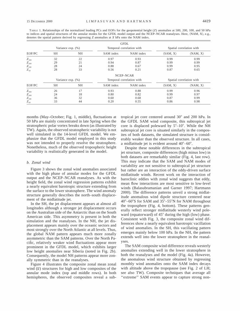
TABLE 1. Relationships of the normalized leading PCs and EOFs for the geopotential height (Z ) anomalies at 500, 200, 100, and 50 hPato indices and spatial structures of the annular modes for the GFDL model output and the NCEP–NCAR reanalyses. Here, ^NAM, X&, e.g.,denotes the spatial pattern derived by regressing Z anomalies at X hPa onto the NAM index.

GFDL

EOF/PC

Variance exp. (%)

SH NH

Temporal correlation with

SAM index NAM index

Spatial correlation with

^SAM, X& ^NAM, X&

Z500

Z200

Z100

Z50

32292828

22212433

0.970.940.880.56

0.930.870.670.21

0.990.990.990.87

0.990.990.950.65

NCEP–NCAR

EOF/PC

Variance exp. (%)

SH NH

Temporal correlation with

SAM index NAM index

Spatial correlation with

^SAM, X& ^NAM, X&

Z500

Z200

Z100

Z50

26243633

17183244

0.930.800.600.20

0.880.820.680.55

0.990.990.870.86

0.960.970.990.98

months (May–October; Fig. 1, middle), fluctuations at50 hPa are mainly concentrated in late Spring when thestratospheric polar vortex breaks down (as illustrated byTW). Again, the observed stratospheric variability is notwell simulated in the 14-level GFDL model. We em-phasize that the GFDL model employed in this studywas not intended to properly resolve the stratosphere.Nonetheless, much of the observed tropospheric heightvariability is realistically generated in the model.

b. Zonal wind

Figure 3 shows the zonal wind anomalies associatedwith the high phase of annular modes for the GFDLoutput and the NCEP–NCAR reanalyses. As with theheight field, the zonal wind regression patterns exhibita nearly equivalent barotropic structure extending fromthe surface to the lower stratosphere. The wind anomalystructure generally describes the north–south displace-ment of the midlatitude jet.

In the SH, the jet displacement appears at almost alllongitudes although a stronger jet displacement occurson the Australian side of the Antarctic than on the SouthAmerican side. This asymmetry is present in both thesimulation and the reanalyses. In the NH, the jet dis-placement appears mainly over the oceanic sectors andmost strongly over the North Atlantic at all levels. Thus,the global NAM pattern appears much more zonallyasymmetric than the SAM patterns. Over the North Pa-cific, relatively weaker wind fluctuations appear moreprominent in the GFDL model, which exhibits largerlow height anomalies near Siberia (noted in Fig. 2b).Consequently, the model NH patterns appear more zon-ally symmetric than in the reanalyses.

Figure 4 illustrates the composite zonal mean zonalwind (u) structures for high and low composites of theannular mode index (top and middle rows). In bothhemispheres, the observed composites reveal a sub-

tropical jet core centered around 308 and 200 hPa. Inthe GFDL SAM wind composite, this subtropical jetcore is displaced poleward by 58–108. While the NHsubtropical jet core is situated similarly in the compos-ites of both datasets, the simulated structure is consid-erably weaker than the observed structure. In all cases,a midlatitude jet is evident around 408–608.

Despite these notable differences in the subtropicaljet structure, composite differences (high minus low) inboth datasets are remarkably similar (Fig. 4, last row).This may indicate that the SAM and NAM modes ofvariability are not sensitive to subtropical jet structurebut rather are an interaction of the eddy-driven surfacemidlatitude winds. Recent work on the interaction ofbaroclinic eddies with zonal wind suggests that eddy,mean flow interactions are most sensitive to low-levelwinds (Balasubramanian and Garner 1997; Hartmann2000). The difference patterns unveil a strong midlat-itude anomalous wind dipole structure centered near408–608S for SAM and 358–558N for NAM throughoutthe troposphere (Fig. 4, bottom). These patterns gen-erally reflect stronger midlatitude westerly wind pole-ward (equatorward) of 458 during the high (low) phase.Consistent with Fig. 3, the composite zonal wind dif-ferences show a nearly equivalent barotropic vacillationof wind anomalies. In the SH, this vacillating patternemerges mainly below 100 hPa. In the NH, the patternextends well into the lower stratosphere in the reanal-yses.

The SAM composite wind difference reveals westerlyanomalies extending well in the lower stratosphere inboth the reanalyses and the model (Fig. 4a). However,the anomalous wind structure obtained by regressingmonthly wind anomalies onto the SAM index decayswith altitude above the tropopause (see Fig. 2 of LH;see also TW). Composite techniques that average all‘‘extreme’’ SAM events appear to capture strong non-


FIG. 4. (a) SAM zonal mean zonal wind composites for the (left) GFDL model and the (right) NCEP–NCAR reanalyses results: (top) highphase composite, (middle) low phase composite, and (bottom) their difference. Contour interval is 5 m s21 for the composites and 1 m s21

for their difference. Negative values are shaded; zero contour is given by the dotted line. Composite difference of the meridional circulationis superimposed in the bottom panel as vectors. The longest vector is about 0.75 m s21. The dipole centers of the composite zonal winddifference are approximated by the vertical dashed lines.

linear features that manifest themselves in the lowerstratosphere.

The anomalous meridional circulation is generallysimilar in both datasets (see arrows in Fig. 4, bottom)and describes the modulation of the Ferrel circulation.As noted by LH and TW, the strongest anomalous sink-ing motion appears around the node of the dipole struc-ture in anomalous zonal wind. Near the surface, stronganomalous meridional winds diverge away from 458 lat,and the associated Coriolis acceleration balances theeffect of surface friction on the anomalous zonal winds.In the upper troposphere, strong anomalous meridionalwinds converge toward 458 lat, and the associated Cor-iolis acceleration is balanced by eddy momentum fluxconvergence. Thus, eddy momentum fluxes in the uppertroposphere appear to be important in maintaining thewind anomalies aloft, and in maintaining the mean me-

ridional circulation that supports the surface wind anom-alies against friction (Hartmann and Lo 1998). We ex-plore the role of eddy forcing in the next section.

4. Zonal-mean eddy forcing and propagation

We compute composites of the eddy forcing of mo-mentum using the Eliassen–Palm (EP) flux divergence(Edmon et al. 1980; Andrews et al. 1987). Forcing dueto meridional divergence of eddy momentum fluxes(‘‘barotropic’’ forcing) and vertical divergence of eddyheat fluxes (‘‘baroclinic’’ forcing) make up the EP fluxdivergence (e.g., Hartmann and Lo 1998). The eddiescan be divided into stationary waves, defined as zonalasymmetries in the monthly means, and transient waves,defined as the deviations from the monthly means. The


FIG. 4. (b) Same as (a) except for the NAM composites.

total eddy forcing includes both stationary wave andtransient wave contributions.

The meridional cross sections of the anomalous eddybarotropic forcing are illustrated in the top panels ofFig. 5. The prevailing structure of the momentum fluxconvergence is a midlatitude dipole located near 300hPa, which indicates a relatively stronger poleward eddymomentum flux across 458 lat during the high phase ofthe NAM and SAM. In the SH, the high-latitude forcinganomaly in the GFDL result exceeds that of the re-analyses.

The centers of the anomalous barotropic forcing di-pole nearly coincide with the latitude of the zonal windanomalies shown in Fig. 4 (bottom). For convenience,the dipole centers of the zonal wind anomalies areshown as vertical dashed lines in Fig. 5. As discussedin section 3, forcing by the eddy momentum fluxes ap-pears to maintain the wind anomalies in the upper tro-posphere and balance the Coriolis torques associated

with the anomalous mean meridional circulation (seealso Fig. 6, bottom).

The properties of the barotropic eddy forcing can besummarized by vertically averaging the forcing between700 and 100 hPa. The solid line in middle panels ofFig. 5 displays the resulting meridional profile. Wechose not to extend the averaging process down to 1000hPa to avoid the strong forcing dipole near the surfaceat 358N in the GFDL result. This dipole pattern is ap-parently a spurious result of our interpolation from sig-ma to pressure surfaces in the region of the Himalayas(Fig. 5b, upper left).

Decomposing the anomalous barotropic eddy forcingprofile into its stationary and transient components re-veals that the forcing is partitioned similarly in bothdatasets but differently in each hemisphere (see dottedand dashed lines in Fig. 5, middle). In the SH, barotropicforcing by the transients dominates over the stationarywave contribution; the transient forcing profile is nearly


FIG. 5. (a) (top) SAM composite difference of the forcing due to eddy momentum flux divergence. Easterly acceleration is shaded. Contourinterval is 0.25 m s21 day21; zero contour is omitted. Vertical dashed lines roughly mark the dipole centers of the zonal wind anomaliesshown in Fig. 4. (middle) Vertically averaged (700–100 hPa) forcing due to eddy momentum flux divergence (solid line). Contributions fromstationary wave and transient components are overlaid. (bottom) Decomposition of the transient part into the high-frequency (HF; ,10 day)and middle frequency (MF; 10–60 day) parts.

identical to the total barotropic eddy forcing profile. Thestationary wave forcing is largest around 708S. In theNH, the stationary wave contribution accounts for aconsiderable fraction of the anomalous wind accelera-tion. The strongest stationary wave forcing is foundaround 608N. Transient eddy forcing also makes an im-portant contribution, particularly equatorward of 458N.The relative importance of eddy forcing due to station-ary waves and transient eddy in the NH is consistentwith the results of DN.

The bottom panels of Fig. 5 show the separation ofthe transient barotropic forcing into its high-frequency

(,10 day) and middle-frequency (10–60 day) parts.Clearly, high-frequency transients associated with syn-optic waves govern much of the total transient forcing.Middle-frequency forcing can be sizeable (especially inNH), and its presence tends to oppose the effects of thehigh-frequency transients.

Composites of the total eddy forcing (barotropic andbaroclinic components) are demonstrated in Fig. 6 (toptwo rows). The total eddy forcing composites (contours)appear similar between both datasets. However, the eddyforcing amplitude in the GFDL results consistently ex-ceeds that in the reanalyses. In both hemispheres, the


FIG. 5. (b) Same as (a) except for the NAM composite difference.

eddy forcing due to converging EP fluxes (negative con-tours) in the middle to upper troposphere around 508–608 is generally stronger during the low phase.

Comparing the top rows of Fig. 5 with the third rowof Fig. 6 yields insights into the role of eddy heat fluxesassociated with the baroclinic eddy forcing component.With the exception of the observed SAM result (Fig.6a, third row, right column), the anomalous total eddyforcing structure embodies much of the barotropic forc-ing shown in Fig. 5 (top row). This similarity attests tothe importance of eddy momentum fluxes in the uppertroposphere. Nonetheless, at these levels, baroclinic ef-fects can enhance the anomalous easterly accelerationnear 358. The baroclinic contribution is generally largestbelow 300 hPa and accounts for the vertical tilt in thestructure of the total anomalous eddy forcing. Above

200 hPa, its effects can lead to strong westerly forcingin the high-latitude middle stratosphere (e.g., Fig. 6b,third row, right column). The inclusion of the baroclinicforcing component also tends to better align the centersof the anomalous eddy forcing with the dipole centersof the zonal wind anomalies in the upper troposphere(compare third row of Fig. 6 with top row of Fig. 5).

In the reanalyses momentum budget for SAM (Fig.6a, third row, right column), the westerly accelerationcenter of the barotropic forcing near 300 hPa is washedout by the baroclinic term. Consequently, the differencepattern at 300 hPa differs markedly from the differencepattern for barotropic forcing. Nonetheless, the overalldifference pattern in the upper troposphere is still qual-itatively similar to the simulated SAM results.

The latitudinal positions of the anomalous total eddy


FIG. 6. (a) SAM composites of the total eddy forcing and their difference. Contour interval for the composites (their difference) is 1.5(0.25) m s21 day21. Negative values (denoting easterly acceleration) are shaded and zero contour is omitted. Eliassen–Palm flux vectors(divided by the background density) are superimposed on the plots. The longest composite vector is 1.4 3 108 m3 s22. Vertical dashed linesroughly mark the dipole centers of the zonal wind anomalies shown in Fig. 4. (bottom) Composite difference of the sum of the total eddyforcing and Coriolis forcing due to mean meridional circulation (thin contour). Composite difference of the zonal wind anomalies shown inFig. 4 (bottom) is repeated in thick contours.

forcing centers tend to align with the zonal wind anom-alies shown in Fig. 4 above 500 hPa. This correspon-dence underlines the importance of eddies in maintain-ing the wind anomalies in the upper troposphere. Inaddition, the sum of the anomalous total eddy forcingand the Coriolis forcing due to anomalous mean me-

ridional circulation is small everywhere except near thesurface (see Fig. 6, bottom), further illustrating the im-portance of the associated anomalous mean meridionalcirculation in sustaining the surface wind anomaliesagainst friction (as noted in Fig. 4, bottom). These con-nections have been discussed previously by Yu and


FIG. 6. (b) Same as (a) except for the NAM composites. The longest composite vector is 4.9 3 108 m3 s22.

Hartmann (1993) and Hartmann and Lo (1998) in theSH and by DN in the NH.

The arrows in Fig. 6 represent the EP flux vectors,which approximate the direction of wave energy prop-agation. The EP flux vectors in the GFDL compositeslargely parallel those in the reanalyses. In both hemi-spheres, the wave activity emanating from the lowerboundary tends to propagate equatorward upon reachingthe tropopause. Equatorward propagation is strongerduring the high phase since a significant amount of en-

ergy during the low phase tends to veer poleward. Dif-ferences between low and high phases are present at alllevels but are most obvious between 600 and 200 hPa.The difference arrows mainly point equatorward, in-dicating anomalous poleward eddy momentum flux inthe high phase.

As shown in Fig. 4, the difference plots of the zonalmean zonal wind NAM and SAM composites appearquite similar. Both describe the meridional shift of thejet throughout the troposphere although the SAM struc-


FIG. 7. The 500-hPa composite difference of the geopotential heightstationary wave. Contour interval is 20 m. Zero contour is omitted.Negative values are shown by connected dashed contour.

ture is centered slightly more poleward. Our results inFig. 5 demonstrate that the maintenance of zonally sym-metric anomalous wind structures are however domi-nated by different types of eddies in each hemisphere.This difference reflects the contrast in land–sea distri-bution between the NH and SH. Thus, while the zonallysymmetric components of the NAM and SAM appearalike, they are fundamentally different.

The NAM composite difference of the stationarywave pattern is shown in Fig. 7 for the model and thereanalyses. Notable differences are found over the oce-anic sectors. The model results have a more pronouncedfluctuation over the North Pacific while the reanalysesresults show stronger changes over the North Atlantic.Regardless of the these differences, the overall struc-tures are remarkably similar in both datasets despite theabsence of anomalous SST in the model. These patternsare also in good agreement with the anomalous station-ary wave responses to midlatitude u variations between358N and 558N shown by Ting et al. (1996, see theirFig. 6a).

In agreement with DN, our study suggests that theseanomalous stationary wave patterns along with the as-

sociated anomalous synoptic waves act to support thezonal flow anomalies characterized by NAM. As shownin LH for the GFDL results (see their Fig. 3), globalpatterns of anomalous NH stationary and synoptic waveactivity indicate synergetic eddy momentum forcingmainly over the oceanic sector in support of the NAMzonal wind anomalies shown in Fig. 3b. On the otherhand, Ting et al. (1996) and DeWeaver and Nigam(2000b) suggest these stationary wave patterns may alsobe maintained to some extent by the midlatitude jetfluctuation through zonal-eddy coupling. Thus, a two-way, reciprocal relationship (i.e., positive feedback in-teraction) between the stationary waves and zonal windanomalies may be at work, as perhaps first suggestedby Kodera et al. (1991) and recently by DeWeaver andNigam (2000b).

5. Index of refraction arguments

We attempt to account for the wave energy propa-gation in NH with the quasigeostrophic refractive index(n2) as given in Chen and Robinson (1992):

2 2q s fw2n 5 2 2 , (5.1)1 2 1 2u 2 (as cosw)/s a cosw 2NH

where

2(u cosw)2V 1 f uw zq 5 cosw 2 2 r . (5.2)w 02 21 2[ ]a a cosw r Nw 0 z

Here, s is the zonal wavenumber, s is the wave fre-quency (radian per second), N 2 is the buoyancy fre-quency, H is the scale height (7 km), f is the Coriolisparameter, a and V are the earth’s radius and angularfrequency, r0 is the background density, and w is lati-tude. Theoretically, the wave activity can propagate inregions of positive refractive index and avoid negativevalues (Andrews et al. 1987). In addition, the waveactivity tends to be refracted toward large positive indexvalues.

Figure 8 shows the NAM refractive indices for thelargest stationary wave (zonal wavenumber 1). Recallthat, in the NH, anomalous eddy momentum forcing ismainly due to stationary waves (e.g., Fig. 5b). The mostprominent characteristic of the refractive index is thelocal maximum situated in the high latitudes just belowthe tropopause. According to WKBJ theory (Andrewset al. 1987), this index of refraction maximum shouldtend to attract waves toward the polar region, givingrise to equatorward momentum fluxes. During the lowphase of the annular mode, this index of refraction max-imum is considerably stronger than during the highphase, as evident by the large negative regions near658N in the composite difference (bottom row of Fig.8).

Analogous variation in stationary wave energy prop-agation in relation to the anomalous shifting of the back-ground jet (and associated index of refraction) was mod-


FIG. 8. NAM composites and their difference of the nondimensionalized quasigeostrophic refractive index (a2n2) for zonal wavenumber1 stationary wave. Contour intervals for the composites (differences) are 50 (40). Negative values are lightly shaded. Heavily shaded arearepresents region where the refractive index is greater or equal to 400.

eled by Nigam and Lindzen (1989). They demonstratedthat slight equatorward displacement of the subtropicaljet (somewhat like the equatorward jet displacementduring the low NAM phase) produces increased sta-tionary wave propagation into higher latitudes of thetroposphere and lower stratosphere (see their Fig. 16).However, the anomalous dipole structure of the windperturbations in their study had a node that is about 108closer to the equator than the dipole structure of theNAM (see bottom of Fig. 4b).

Detailed examination shows that the anomalous localmaximum structure in the refractive index shown at thebottom of Fig. 8 is most sensitive to the term relatedto vertical zonal wind shear. Excluding both the secondand third terms in the right-hand side (rhs) of (5.2) doesnot yield the negative extrema near 6 km in the com-posite difference pattern shown in Fig. 8. Exclusion ofthe third term in the rhs of (5.1) also fails to generate

the local negative extrema. We find that the third termin the rhs of (5.2) accounts for most of the differencein n2 between the high and low phases. Expansion ofthis third term into ( f 2/r0)(r0/N 2)zu z and ( f 2/r0)(r0/N 2)uzz reveals that the former quantity, which is relatedto the vertical wind shear, is most important.

As displayed in Fig. 4, the zonal flow during the highphase of the annular mode exhibits considerably stron-ger westerly winds and westerly vertical wind shear (i.e.,zonal wind increasing with altitude) than the low phasebetween 608 and 808N. The stronger westerly windsduring the high phase cause waves to be less stronglyrefracted toward the pole, resulting in anomalous equa-torward wave propagation and poleward momentumanomalies. The poleward momentum anomalies in turnsupport the high-latitude westerlies. In the model, high-latitude vertical wind variation is generally much weak-er than observation in both high and low phases. Con-


sequently, high-latitude regions of very large refractiveindex values (heavily shaded) are found in both phasesof the model results.

The numerical study of Chen and Robinson (1992)found that strong vertical wind shear also impedes thevertical propagation of planetary waves across the tro-popause. One might reasonably speculate that duringthe high phase, propagation of planetary waves into thestratosphere would be inhibited relative to the lowphase. Since planetary waves tend to break in the strato-sphere upon reaching their critical surfaces and weakenthe polar vortex, one would expect that the polar vortexwill be stronger when the tropospheric annular mode isin its positive phase. When the tropospheric jet is dis-placed equatorward in the low phase, one would expectmore planetary wave activity in the stratosphere and aweaker polar vortex. These associations between tro-pospheric annular variability and stratospheric vari-ability are essentially what has been described by Bald-win and Dunkerton (1999) and TW and occur both inmonth-to-month variability and in decadal trends.

6. Summary

The annular modes are identified in a 100-yr controlrun of the GFDL GCM as the leading modes of tro-pospheric month-to-month variability. In this simula-tion, the model’s lower boundary is prescribed only withrealistic topography and seasonally varying climatolog-ical SST. The simulated annular modes are shown to bevery similar to those found in the NCEP–NCAR re-analyses, which includes the influence of SST interan-nual variability. Similarities between the model and re-analyses results confirm that the annular modes cantherefore be produced entirely by internal atmosphericdynamical processes.

The characteristics of the annular modes presented hereare very similar to those of recent studies by Baldwinand Dunkerton (1999) and TW who employed slightlydifferent annular mode indices. Throughout the entiretroposphere, the mode is dominated by a near zonallysymmetric, meridional displacement of the jet as the polarvortex expands and contracts. The NAM spatial structureis nearly identical to the widely known NAO and, to thisend, we consider them to be one and the same phenom-enon (Wallace 2000). While the NAM features are dom-inated by a higher degree of zonal variations, the zonallysymmetric components of the NAM and SAM are re-markably similar. The annular mode zonal mean zonalwind anomalous structure describes the meridional trans-lation of the jet and associated expansion/contraction ofthe vortex. Strongest mode variance occurs during thecold months. This seasonal variation is very pronouncedin the NH.

From composites based on the annular mode index,anomalous eddy forcing appears to maintain the zonalmean zonal wind anomalies associated with the annularmodes in both model and reanalyses. Anomalous di-

vergence of eddy momentum fluxes plays a large rolein sustaining the wind anomalies in the upper tropo-sphere while the Coriolis acceleration associated withanomalous mean meridional circulation sustains thenear-surface wind anomalies against frictional dissipa-tion. The anomalous eddy forcing reflects differencesin the pattern of eddy propagation in the upper tropo-sphere during the extreme phases of the annular mode.In the high phase, eddy energy propagates almost ex-clusively equatorward at these altitudes. Weaker equa-torward propagation is evident during the low phase.

The type of eddy most responsible for the changedmomentum fluxes that sustain the zonally symmetriccomponent of the annular modes is different in the South-ern and Northern Hemispheres. In the SH, high-frequen-cy (synoptic) transients are mostly responsible for thewind anomalies, in agreement with past studies on SHflow vacillation (e.g., Hartman and Lo 1998; Karoly1990). In the NH, eddy forcing due to stationary wavesis most important, particularly around 608N and in theAtlantic sector. High-frequency transients also make im-portant contribution to the maintenance of the windanomalies in the NH equatorward of 458N. Thus, al-though the zonally symmetric component of the NAMand SAM are remarkably similar, they are fundamentallydifferent as they are mostly maintained by different typesof eddies. This difference ultimately reflects the contrast-ing land–sea distribution in the two hemispheres.

A first-order understanding of the interaction betweenNAM and stationary wave propagation can be derivedfrom WKBJ theory relating the background wind withwave refractive properties. In the high phase, planetaryRossby waves are less strongly refracted toward the pole,so that they mainly propagate equatorward. This equa-torward propagation is associated with poleward mo-mentum fluxes, which help to sustain the poleward dis-placement of tropospheric westerlies associated with thehigh NAM phase. In the low phase, stationary waves aremore strongly attracted toward the polar regions, yieldingan anomalous equatorward momentum flux. The in-creased refractive index values in high latitudes that at-tract planetary waves poleward in the low index case areassociated primarily with weaker vertical wind shear inthe high-latitude upper troposphere during the low phase.

The planetary wave propagation characteristics can beused to link changes in the tropospheric annular modeto changes in the strength of the stratospheric polar vortexduring winter. Planetary waves are strongly attracted topolar regions during the low phase of the annular modewhen the tropospheric westerlies are displaced equator-ward. We should expect a weaker stratospheric polar vor-tex then, since planetary waves weaken the polar vortexby generating irreversible mixing. This association of lowNAM phase with a weakened wintertime stratosphericvortex is indeed observed. Recently, Baldwin and Dunk-erton (1999) and Hartmann et al. (2000) illustrate thatmajor stratospheric warming occurs almost exclusivelyduring the low NAM phase due to the increased station-


ary wave activity in the lower stratosphere. When thetropospheric midlatitude westerlies are displaced towardthe pole, planetary waves are refracted equatorward, lessplanetary wave activity propagates upward at high lati-tudes, and we should expect the stratospheric vortex tobe stronger.

Finally, we reiterate that our composite results arebased on an index derived from monthly EOF analysis.In the NH, composites computed using all months withextreme index values (exceeding 61.5 standard devi-ation) are found to be very similar to composites inwhich only the winter months (December–March) areemployed. This is because extreme NAM index valuesare mostly found during the winter season as suggestedby Fig. 1 (middle). We did not perform EOF analysisbased only on the winter months. We expect the com-posites based on the analysis of the winter data wouldbe similar to the results presented here, however.

Acknowledgments. This research was supported bythe NOAA/GFDL Universities Consortium grant (JointInstitute for the Study of the Atmosphere and Oceancontribution number 703). The authors thank Drs. J. M.Wallace and C. B. Leovy and our colleagues in theconsortium for their interests and helpful discussions.Mary Jo Nath at GFDL and Marc Michelsen are alsoacknowledged for their computing assistance. The com-ments of Dr. Sumant Nigam and an anonymous reviewercontributed significantly to the improvement of the orig-inal manuscript.

REFERENCES

Andrews, D. G., J. R. Holton, and C. B. Leovy, 1987: Middle At-mosphere Dynamics. Academic Press, 498 pp.

Balasubramanian, G., and S. T. Garner, 1997: The role of momentumfluxes in shaping the life cycles of a baroclinic wave. J. Atmos.Sci., 54, 510–533.

Baldwin, M. P., and T. J. Dunkerton, 1999: Propagation of the arcticoscillation from the stratosphere to the troposphere. J. Geophys.Res., 104, 30 937–30 946.

Chen, P., and W. A. Robinson, 1992: Propagation of planetary wavesbetween the troposphere and stratosphere. J. Atmos. Sci., 49,2533–2545.

DeWeaver, E., and S. Nigam, 2000a: Do stationary waves drive thezonal-mean jet anomalies of the northern winter? J. Climate, 13,2160–2176., and , 2000b: Zonal-eddy dynamics of the North AtlanticOscillation. J. Climate, 13, 3893–3914.

Edmon, H. J., Jr., B. J. Hoskins, and M. E. McIntyre, 1980: Eliassen–Palm cross sections for the troposphere. J. Atmos. Sci., 37, 2600–2616.

Gordon, C. T., and W. F. Stern, 1982: A description of the GFDLglobal spectral model. Mon. Wea. Rev., 110, 625–644.

Hartmann, D. L., 1995: A PV view of zonal flow vacillation. J. Atmos.Sci., 52, 2561–2576., 2000: The key role of lower-level meridional shear in baroclinicwave life cycles. J. Atmos. Sci., 57, 389–401., and F. Lo, 1998: Wave-driven zonal flow vacillation in theSouthern Hemisphere. J. Atmos. Sci., 55, 1303–1315.

, J. M. Wallace, V. Limpasuvan, D. W. J. Thompson, and J. R.Holton, 2000: Can ozone depletion and global warming interactto produce rapid climate change? Proc. Natl. Acad. Sci., 92,1412–1417.

Hoerling, M. P., M. Ting, and A. Kumar, 1995: Zonal flow-stationarywave relationship during El Nino: Implications for seasonal fore-casting. J. Climate, 8, 1838–1852.

Hurrell, J. W., 1995: Decadal trends in the North Atlantic oscillation:Regional temperatures and precipitation. Science, 269, 676–679.

Kalnay, E., and Coauthors, 1996: The NCEP/NCAR 40-Year Re-analysis Project. Bull. Amer. Meteor. Soc., 77, 437–471.

Karoly, D. J., 1990: The role of transient eddies in low-frequencyzonal variations in the Southern Hemisphere circulation. Tellus,42A, 41–50.

Kidson, J. W., 1988: Indices of the Southern Hemisphere zonal wind.J. Climate, 1, 183–194.

Kodera, K., M. Chiba, K. Yamazaki, and K. Shibata, 1991: A possibleinfluence of the polar night stratospheric jet on the subtropicaltropospheric jet. J. Meteor. Soc. Japan, 69, 715–721.

Lau, N.-C., and M. J. Nath, 1990: A general circulation model studyof the atmospheric response to extratropical SST anomalies ob-served in 1950–79. J. Climate, 3, 965–989.

Limpasuvan, V., and D. L. Hartmann, 1999: Eddies and the annularmodes of climate variability. Geophys. Res. Lett., 26, 3133–3136.

Nigam, S., 1990: On the structure of variability of the observedtropospheric and stratospheric zonal-mean wind. J. Atmos. Sci.,47, 1799–1813., and R. S. Lindzen, 1989: The sensitivity of stationary wavesto variations in the basic state zonal flow. J. Atmos. Sci., 46,1746–1768.

North, G. R., T. L. Bell, R. F. Cahalan, and F. J. Moeng, 1982: Sam-pling errors in the estimation of empirical orthogonal functions.Mon. Wea. Rev., 110, 699–706.

Robinson, W. A., 1991: The dynamics of the zonal index in a simplemodel of the atmosphere. Tellus, 43A, 295–305.

Rodgers, J. C., 1984: Association between the North Atlantic oscil-lation and the Southern Oscillation in the Northern Hemisphere.Mon. Wea. Rev., 112, 1999–2015., and H. van Loon, 1982: Spatial variability of sea level pressureand 500-mb height anomalies over the Southern Hemisphere.Mon. Wea. Rev., 110, 1375–1392.

Shiotani, M., 1990: Low-frequency variations of the zonal mean stateof the Southern Hemisphere troposphere. J. Meteor. Soc. Japan,68, 461–470.

Thompson, D. W. J., and J. M. Wallace, 1998: The Arctic oscillationsignature in the wintertime geopotential height and temperaturefields. Geophys. Res. Lett., 25, 1297–1300., and , 2000: Annual modes in the extratropical circulation.Part I: Month-to-month variability. J. Climate, 13, 1000–1016., , and G. Hegerl, 2000: Annual modes in the extratropicalcirculation. Part II: Trends. J. Climate, 13, 1018–1036.

Ting, M., M. P. Hoerling, T. Xu, and A. Kumar, 1996: NorthernHemisphere teleconnection patterns during extreme phases ofthe zonal-mean circulation. J. Climate, 9, 2614–2633.

Trenberth, K. E., 1984: Interannual variability of the Southern Hemi-sphere circulation: Representativeness of the year of the GlobalWeather Experiment. Mon. Wea. Rev., 112, 108–125.

Wallace, J. M., 2000: North Atlantic oscillation/annular mode: Twoparadigms—one phenomenon. Quart. J. Roy. Meteor. Soc., 126,791–805., and H.-H. Hsu, 1985: Another look at the index cycle. Tellus,37A, 478–486.

Yoden, S., M. Shiotani, and I. Hirota, 1987: Multiple planetary flowregimes in the Southern Hemisphere. J. Meteor. Soc. Japan, 65,571–585.

Yu, J.-Y., and D. L. Hartmann, 1993: Zonal flow vacillation and eddyforcing in a simple GCM of the atmosphere. J. Atmos. Sci., 50,3244–3259.

Wave-Maintained Annular Modes of Climate Variability

Documents

Transcript of Wave-Maintained Annular Modes of Climate Variability