Watershed Sciences 6900FLUVIAL HYDRAULICS & ECOHYDRAULICS

FORCES & FLOW CLASSIFICATION + ENERGY & MOMENTUM PRINCIPLES

Joe Wheaton

Slides by Wheaton et al. (2009-2014) are licensed under a Creative Commons Attribution-NonCommercial-ShareAlike 3.0 Unported License

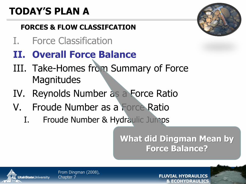
TODAY’S PLAN A

I. Force Classification

II. Overall Force Balance

III. Take-Homes from Summary of Force Magnitudes

IV. Reynolds Number as a Force Ratio

V. Froude Number as a Force Ratio

I. Froude Number & Hydraulic Jumps

FORCES & FLOW CLASSIFCATION

From Dingman (2009)

WE’VE ALREADY DEALT WITH FORCES… BUT:

• Understanding the relative magnitudes of all forces in different situations gives us a basis for ignoring them… (i.e. simplifying assumptions)

• To keep comparison simple, consider:

Wide, rectangular channel (Y=R) with constant width (W1=W2=W) but

spatially variable depth

𝐹𝐷 = 𝐹𝑅 𝐹 = 𝑚 ∙ 𝑎

From Dingman (2008), Chapter 7

TODAY’S PLAN A

I. Force Classification

II. Overall Force Balance

III. Take-Homes from Summary of Force Magnitudes

IV. Reynolds Number as a Force Ratio

V. Froude Number as a Force Ratio

I. Froude Number & Hydraulic Jumps

FORCES & FLOW CLASSIFCATION

From Dingman (2008)

A SIMPLE FORCE CLASSIFICATION

𝐹 = 𝑚 ∙ 𝑎 a= 𝐹

𝑚

Forces per unit mass…

From Dingman (2008), Chapter 7

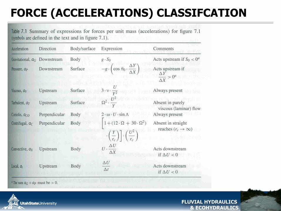
FORCE (ACCELERATIONS) CLASSIFCATION

TODAY’S PLAN A

I. Force Classification

II. Overall Force Balance

III. Take-Homes from Summary of Force Magnitudes

IV. Reynolds Number as a Force Ratio

V. Froude Number as a Force Ratio

I. Froude Number & Hydraulic Jumps

FORCES & FLOW CLASSIFCATION

What did Dingman Mean by Force Balance?

From Dingman (2008), Chapter 7

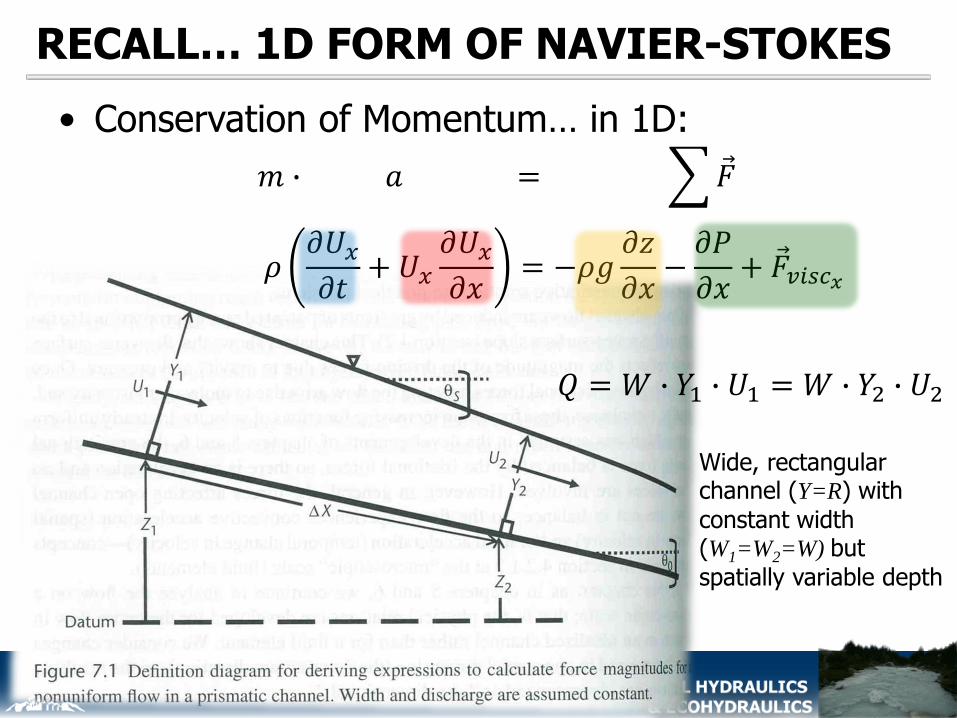
RECALL… 1D FORM OF NAVIER-STOKES

• Conservation of Momentum… in 1D:

𝑚 ∙ 𝑎 = 𝐹

𝜌𝜕𝑈𝑥𝜕𝑡+ 𝑈𝑥𝜕𝑈𝑥𝜕𝑥= −𝜌𝑔

𝜕𝑧

𝜕𝑥−𝜕𝑃

𝜕𝑥+ 𝐹𝑣𝑖𝑠𝑐𝑥

𝑄 = 𝑊 ∙ 𝑌1 ∙ 𝑈1 = 𝑊 ∙ 𝑌2 ∙ 𝑈2

Wide, rectangular channel (Y=R) with

constant width (W1=W2=W) but

spatially variable depth

SO IN TERMS OF a= 𝐹

𝑚CLASSIFICATION

𝜌𝜕𝑈𝑥𝜕𝑡+ 𝑈𝑥𝜕𝑈𝑥𝜕𝑥= −𝜌𝑔

𝜕𝑧

𝜕𝑥−𝜕𝑃

𝜕𝑥+ 𝐹𝑣𝑖𝑠𝑐𝑥

𝜕𝑈𝑥𝜕𝑡+ 𝑈𝑥𝜕𝑈𝑥𝜕𝑥= −𝑔𝜕𝑧

𝜕𝑥−1

𝜌∙𝜕𝑃

𝜕𝑥+ 𝐹𝑣𝑖𝑠𝑐𝑥𝜌

𝑎𝑡 + 𝑎𝑋 = −𝑎𝐺 − 𝑎𝑃 + 𝑎𝑉

1D Momentum Equation…

Rearranged in terms of our

classification…

Matched to Table 7.1

From Dingman (2008), Chapter 7

RECALL: DEFINITIONS OF UNIFORM & STEADY FLOW

• Uniform Flow: if the element velocity at any instant is constant along a streamline the flow is uniform (i.e. convective acceleration 𝑑𝑢 𝑑𝑥 = 0),.

• Steady Flow: if the element velocity 𝑢 at any

given point on a streamline does not change with time, the flow is steady (i.e. local acceleration 𝑑𝑢 𝑑𝑡 = 0) .

From Dingman (2008) – Chapter 4& 6

THREE MAIN OPEN CHANNEL FLOW TYPES

1. Steady Uniform Flow

2. Steady Nonuniform Flow

3. Unsteady Nonuniform Flow

𝑎𝑡 + 𝑎𝑋 = −𝑎𝐺 − 𝑎𝑃 + 𝑎𝑉𝑎𝐺 + 𝑎𝑃 − 𝑎𝑉 + 𝑎𝑇 + 𝑎𝑋 + 𝑎𝑡 = 0

𝐹𝐷 = 𝐹𝑅

• Downstream forces (+): 𝐹𝐷• Upstream Forces (-): 𝐹𝑅

𝑎𝐺 − 𝑎𝑉 + 𝑎𝑇 = 0 EQ 7.2

EQ 7.3

EQ 7.4

𝑎𝐺 + 𝑎𝑃 − 𝑎𝑉 + 𝑎𝑇 + 𝑎𝑋 = 0

• Steady/Unsteady (Time)• Uniform/Nonuniform (Space)

𝑎𝐺 + 𝑎𝑃 − 𝑎𝑉 + 𝑎𝑇 + 𝑎𝑋 + 𝑎𝑡 = 0

𝑎𝐺 + 𝑎𝑃 − 𝑎𝑉 + 𝑎𝑇 = 𝑎𝑋

𝑎𝐺 + 𝑎𝑃 − 𝑎𝑉 + 𝑎𝑇 = 𝑎𝑋 + 𝑎𝑡

SO WHAT IS NAVIER STOKES?

• Unsteady or Steady?

• Uniform or Nonuniform?

𝜌𝜕𝑈𝑥𝜕𝑡+ 𝑈𝑥𝜕𝑈𝑥𝜕𝑥= −𝜌𝑔

𝜕𝑧

𝜕𝑥−𝜕𝑃

𝜕𝑥+ 𝐹𝑣𝑖𝑠𝑐𝑥

𝑎𝐺 + 𝑎𝑃 − 𝑎𝑉 + 𝑎𝑇 = 𝑎𝑋 + 𝑎𝑡

𝜕𝑈𝑥𝜕𝑡+ 𝑈𝑥𝜕𝑈𝑥𝜕𝑥= −𝑔𝜕𝑧

𝜕𝑥−1

𝜌∙𝜕𝑃

𝜕𝑥+ 𝐹𝑣𝑖𝑠𝑐𝑥𝜌

𝑎𝑡 + 𝑎𝑋 = −𝑎𝐺 − 𝑎𝑃 + 𝑎𝑉

“The difference between the driving & resisting forces is acceleration.”

𝐹𝐷 ≠ 𝐹𝑅

𝐹𝐷 − 𝐹𝑅 = 𝑎EQ 7.4

TODAY’S PLAN A

I. Force Classification

II. Overall Force Balance

III. Take-Homes from Summary of Force Magnitudes

IV. Reynolds Number as a Force Ratio

V. Froude Number as a Force Ratio

I. Froude Number & Hydraulic Jumps

FORCES & FLOW CLASSIFCATION

RANGE OF FORCE VALUES

• Downstream forces (+): 𝐹𝐷• Upstream Forces (-): 𝐹𝑅

• Body Forces

• Surface Forces

TODAY’S PLAN A

I. Force Classification

II. Overall Force Balance

III. Take-Homes from Summary of Force Magnitudes

IV. Reynolds Number as a Force Ratio

V. Froude Number as a Force Ratio

I. Froude Number & Hydraulic Jumps

FORCES & FLOW CLASSIFCATION

From Dingman (2008)

REYNOLDS NUMBER

• Can also be shown that 𝑅𝑒 ∝𝑎𝑇

𝑎𝑉(ratio of turbulent

forces to viscous forces):

• So… is it fair to say that Reynolds number is sort of a ratio of driving forces to resisting forces?

• No! Why?

𝑅𝑒 ≡𝜌∙𝑌∙𝑈

𝜇=𝑌∙𝑈

𝜈Ratio of ‘inertial forces’ to viscous forces

𝑎𝑇𝑎𝑉=

Ω2 ∙ 𝜌 ∙ 𝑈2

𝑌3 ∙ 𝜇 ∙ 𝑈𝑌2

=Ω2 ∙ 𝜌 ∙ 𝑈 ∙ 𝑌

3 ∙ 𝜇=Ω2 ∙ 𝑈 ∙ 𝑌

3 ∙ 𝜐=Ω2

3∙ 𝑅𝑒

TODAY’S PLAN A

I. Force Classification

II. Overall Force Balance

III. Take-Homes from Summary of Force Magnitudes

IV. Reynolds Number as a Force Ratio

V. Froude Number as a Force Ratio

I. Froude Number & Hydraulic Jumps

FORCES & FLOW CLASSIFCATION

From Dingman (2008)

FROUDE NUMBER AS A FORCE RATIO

TODAY’S PLAN A

I. Force Classification

II. Overall Force Balance

III. Take-Homes from Summary of Force Magnitudes

IV. Reynolds Number as a Force Ratio

V. Froude Number as a Force Ratio

I. Froude Number & Hydraulic Jumps

FORCES & FLOW CLASSIFCATION

From Dingman (2008)

FROUDE NUMBER

• What are Dimensions?

𝐹𝑟 ≡𝑈

𝑔 ∙ 𝑌 12

Ratio of velocity to

Celerity (𝐶𝑔𝑤 = 𝑔 ∙ 𝑌)

[LT-1]

[LT-2 L]1/2

[LT-2 L]1/2 =LT-1

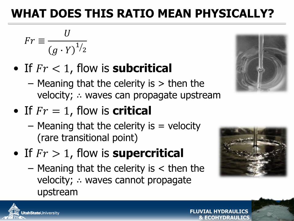
WHAT DOES THIS RATIO MEAN PHYSICALLY?

• If 𝐹𝑟 < 1, flow is subcritical

– Meaning that the celerity is > then the velocity; ∴ waves can propagate upstream

• If 𝐹𝑟 = 1, flow is critical

– Meaning that the celerity is = velocity (rare transitional point)

• If 𝐹𝑟 > 1, flow is supercritical

– Meaning that the celerity is < then the velocity; ∴ waves cannot propagate

upstream

𝐹𝑟 ≡𝑈

𝑔 ∙ 𝑌 12

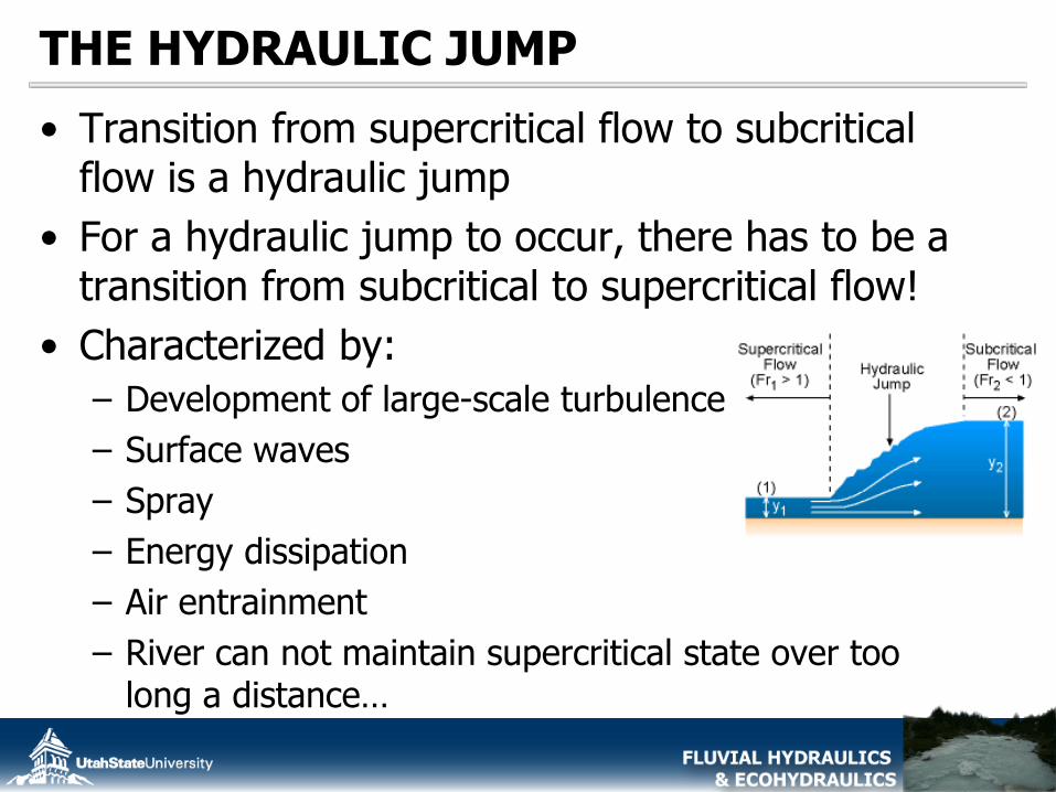
THE HYDRAULIC JUMP

• Transition from supercritical flow to subcritical flow is a hydraulic jump

• For a hydraulic jump to occur, there has to be a transition from subcritical to supercritical flow!

• Characterized by:

– Development of large-scale turbulence

– Surface waves

– Spray

– Energy dissipation

– Air entrainment

– River can not maintain supercritical state over too long a distance…

HYDRAULIC JUMP TYPES…

From Dingman (2008), Chapter 10 & Chanson (2004)

WHY CAN YOU SURF IN A RIVER?

• Explain it in terms of Froude Number…

• Which way is water going? (kayakers can’t answer!)

TODAY’S PLAN B

I. Energy Principle in 1D Flows

I. The Energy Equation (§ 8.1.1)

II. Specific Energy (§ 8.1.2)

ENERGY & MOMENTUM PRINCIPLES (Applied to 1D flows)

From Chanson (2004)

TODAY’S PLAN

I. Energy Principle in 1D Flows

I. The Energy Equation (§ 8.1.1)

II. Specific Energy (§ 8.1.2)

ENERGY & MOMENTUM PRINCIPLES (Applied to 1D flows)

From Dingman (2008), Chapter 8

TOTAL ENERGY 𝒉 (FROM §4.4)

• The total energy ℎ of an element is the sum of its potential energy ℎ𝑃𝐸 & its kinetic energy ℎ𝐾𝐸:

• Recall that ℎ𝑃𝐸 is the sum of gravitational potential energy ℎ𝐺 and pressure potential energy ℎ𝑃 :

• ∴ total energy ℎ is:

From Dingman (2008), Chapter 8

ℎ = ℎ𝑃𝐸 + ℎ𝐾𝐸

ℎ𝑃𝐸 = ℎ𝐺 + ℎ𝑃

ℎ = ℎ𝐺 + ℎ𝑃 + ℎ𝐾𝐸

EQ 8.1

EQ 8.2

Energy quantities are expressed as energy

[F L] divided by weight [F], which is

called head [L]

DEFINITON DIAGRAM FOR ENERGY IN 1D

• Used for derivation of the macroscopic one-dimensional energy equation

• Flow through reach is steady

From Dingman (2008), Chapter 8

TODAY’S PLAN B

I. Energy Principle in 1D Flows

I. The Energy Equation (§ 8.1.1)

II. Specific Energy (§ 8.1.2)

ENERGY & MOMENTUM PRINCIPLES (Applied to 1D flows)

From Dingman (2008), Chapter 8

TOTAL MECHANICAL ENERGY AT A CROSS SECTION

• Based on what Ryan showed us, using the channel bottom as a reference point, at cross section 𝑖 we can

write the integrated gravitational head (AKA elevation head), 𝐻𝐺𝑖:

• Where 𝑍𝑖 is the elevation of the channel bottom, and the integrated pressure head 𝐻𝑃𝑖 is:

• Kinetic energy head 𝐻𝐾𝐸 for a fluid element with velocity 𝑢 is given by:

From Dingman (2008), Chapter 8

𝐻𝐺𝑖 = 𝑍𝑖 EQ 8.3

𝐻𝑃𝑖 = 𝑌𝑖 ∙ 𝑐𝑜𝑠𝜃0 EQ 8.4

ℎ𝐾𝐸 =𝑢2

2 ∙ 𝑔EQ 8.5

VELOCITY COEFFICIENT 𝜶 FOR ENERGY

• Because velocity varies from point to point n a cross section, we need a fudge factor 𝛼𝑖 to account for this

variation, so the velocity head 𝐻𝐾𝐸𝑖 is:

ℎ𝐾𝐸𝑖 =𝛼𝑖 ∙ 𝑈𝑖

2

2 ∙ 𝑔

EQ 8.6

From Dingman (2008), Chapter 8

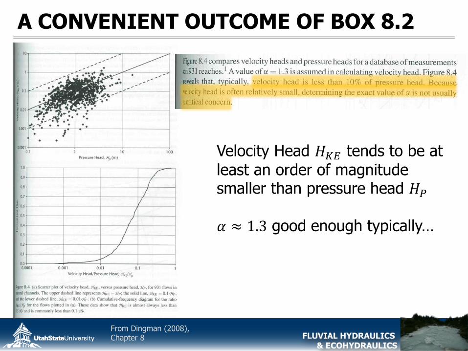
A CONVENIENT OUTCOME OF BOX 8.2

Velocity Head 𝐻𝐾𝐸 tends to be at

least an order of magnitude smaller than pressure head 𝐻𝑃

𝛼 ≈ 1.3 good enough typically…

From Dingman (2008), Chapter 8

TOTAL HEAD 𝑯𝒊 AT A CROSS SECTION 𝒊

• ‘The total mechanical energy-per-weight, or total head 𝐻𝑖, at cross-section 𝑖, is the sum of the gravitational, pressure and velocity heads:

𝐻𝑖 = 𝐻𝐺𝑖 +𝐻𝑃𝑖 +𝐻𝐾𝐸𝑖ℎ = ℎ𝐺 + ℎ𝑃 + ℎ𝐾𝐸

𝐻𝑖 = 𝑍𝑖 + 𝑌𝑖 ∙ 𝑐𝑜𝑠𝜃0 +𝛼𝑖 ∙ 𝑈𝑖

2

2 ∙ 𝑔

From Dingman (2008), Chapter 8

EQ 8.6

But, this is just at one cross section 𝒊… What

about for this diagram?

APPLY 𝑯𝒊 BETWEEN TWO CROSS SECTIONS

• What is the change in in cross-sectional integrated energy from an upstream section (𝑖 = 𝑈) to a downstream section (𝑖 = 𝐷)?

• Where ∆𝐻 is the energy lost

(converted to head) per weigh of fluid, or head loss.

From Dingman (2008), Chapter 8

𝑍𝑈 + 𝑌𝑈 ∙ 𝑐𝑜𝑠𝜃0 +𝛼𝑈∙𝑈𝑈

2

2∙𝑔=𝑍𝐷 + 𝑌𝐷 ∙ 𝑐𝑜𝑠𝜃0 +

𝛼𝐷∙𝑈𝐷2

2∙𝑔+ ∆𝐻

EQ 8.8b

𝐻𝑖 = 𝑍𝑖 + 𝑌𝑖 ∙ 𝑐𝑜𝑠𝜃0 +𝛼𝑖 ∙ 𝑈𝑖

2

2 ∙ 𝑔 EQ 8.6

𝐻𝐺𝑈 + 𝐻𝑃𝑈 + 𝐻𝐾𝐸𝑈 = 𝐻𝐺𝐷 + 𝐻𝑃𝐷 + 𝐻𝐾𝐸𝐷 + ∆𝐻EQ 8.8a

This is the ENERGY EQUATION!

THE ENERGY EQUATION APPLIES WHERE?

• Depth can vary!

• Assumed that pressure distribution was hydrostatic (i.e. streamlines no significantly curved)

• We call this steady gradually varied flow

• This is focus of Chapter 9

• We’ll use it in flume on Thursday!

𝑍𝑈 + 𝑌𝑈 ∙ 𝑐𝑜𝑠𝜃0 +𝛼𝑈∙𝑈𝑈

2

2∙𝑔=𝑍𝐷 + 𝑌𝐷 ∙ 𝑐𝑜𝑠𝜃0 +

𝛼𝐷∙𝑈𝐷2

2∙𝑔+ ∆𝐻

EQ 8.8b

SOME IMPORTANT IMAGINARY LINES

• The line representing the total potential energy from section to section is called the piezometric head line

𝑆𝐸 ≡ −𝐻𝐷−𝐻𝑈

∆𝑋=∆𝐻

∆𝑋= EQ 8.9

• The line representing the total head from section to section is called the energy grade line

• The slope 𝑆𝐸 of the energy grade line is the energy slope:

WOULD THE ENERGY EQUATION APPLY HERE?

• Hint, energy loss..

• Okay.. If it does apply, what would the energy grade line look like for a hydraulic jump?

TODAY’S PLAN B

I. Energy Principle in 1D Flows

I. The Energy Equation (§ 8.1.1)

II. Specific Energy (§ 8.1.2)

ENERGY & MOMENTUM PRINCIPLES (Applied to 1D flows)

From Dingman (2008), Chapter 8

SPECIFIC ENERGY 𝑯𝑺𝒊

• Similar to 𝐻𝑖, just that datum is changed so that mechanical energy is measured with respect to the channel bottom instead of horizontal datum

• Upshot is that elevation head 𝐻𝐺𝑖 → 0 in 𝐻𝑖 = 𝐻𝐺𝑖 +𝐻𝑃𝑖 +𝐻𝐾𝐸𝑖 , such that:

𝐻𝑆𝑖 = 𝐻𝑃𝑖 +𝐻𝐾𝐸𝑖

𝐻𝑆𝑖 = 𝑌𝑖 ∙ 𝑐𝑜𝑠𝜃0 +𝛼𝑖 ∙ 𝑈𝑖

2

2 ∙ 𝑔EQ 8.10

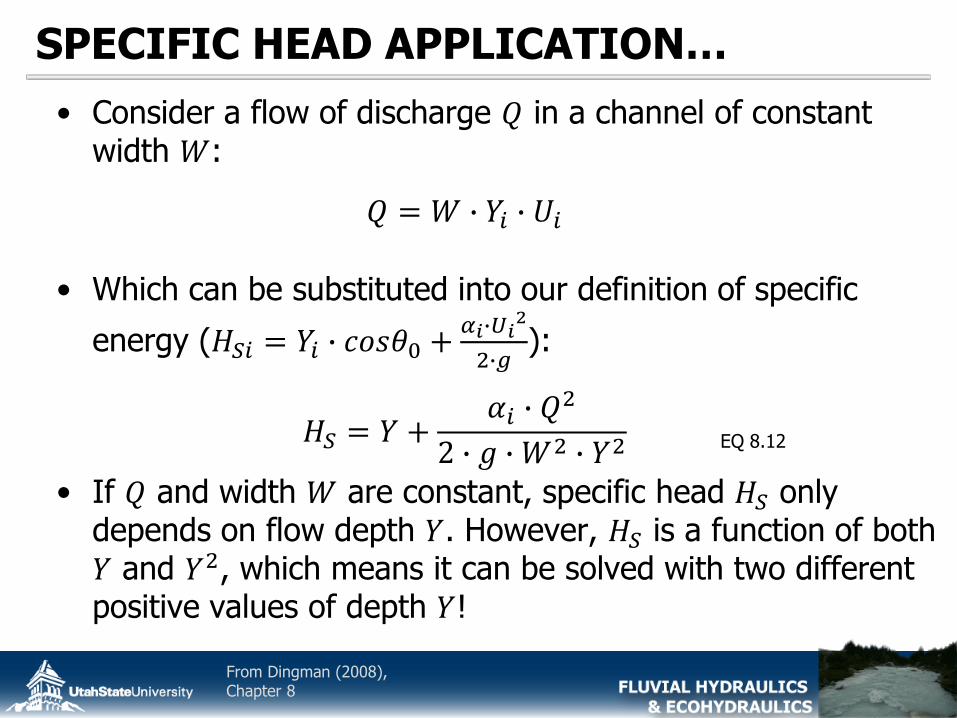
SPECIFIC HEAD APPLICATION…

• Consider a flow of discharge 𝑄 in a channel of constant width 𝑊:

• Which can be substituted into our definition of specific

energy (𝐻𝑆𝑖 = 𝑌𝑖 ∙ 𝑐𝑜𝑠𝜃0 +𝛼𝑖∙𝑈𝑖

2

2∙𝑔):

• If 𝑄 and width 𝑊 are constant, specific head 𝐻𝑆 only depends on flow depth 𝑌. However, 𝐻𝑆 is a function of both 𝑌 and 𝑌2, which means it can be solved with two different positive values of depth 𝑌!

𝑄 = 𝑊 ∙ 𝑌𝑖 ∙ 𝑈𝑖

𝐻𝑆 = 𝑌 +𝛼𝑖 ∙ 𝑄

2

2 ∙ 𝑔 ∙ 𝑊2 ∙ 𝑌2 EQ 8.12

From Dingman (2008), Chapter 8

SPECIFIC HEAD DIAGRAM

𝐻𝑆 = 𝑌 +𝛼𝑖 ∙ 𝑄

2

2 ∙ 𝑔 ∙ 𝑊2 ∙ 𝑌2

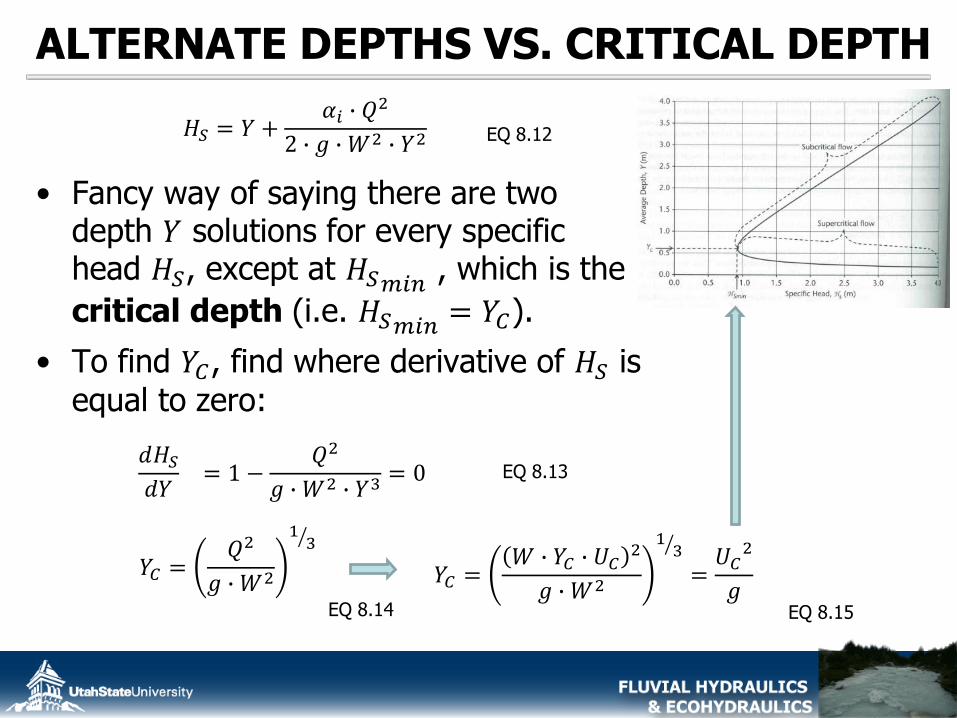
ALTERNATE DEPTHS VS. CRITICAL DEPTH

• Fancy way of saying there are two depth 𝑌 solutions for every specific head 𝐻𝑆, except at 𝐻𝑆𝑚𝑖𝑛 , which is the

critical depth (i.e. 𝐻𝑆𝑚𝑖𝑛 = 𝑌𝐶).

• To find 𝑌𝐶, find where derivative of 𝐻𝑆 is

equal to zero:

𝐻𝑆 = 𝑌 +𝛼𝑖 ∙ 𝑄

2

2 ∙ 𝑔 ∙ 𝑊2 ∙ 𝑌2

𝑑𝐻𝑆𝑑𝑌= 1 −

𝑄2

𝑔 ∙ 𝑊2 ∙ 𝑌3= 0

EQ 8.12

EQ 8.13

𝑌𝐶 =𝑄2

𝑔 ∙ 𝑊2

1 3

EQ 8.14

𝑌𝐶 =𝑊 ∙ 𝑌𝐶 ∙ 𝑈𝐶

2

𝑔 ∙ 𝑊2

1 3

=𝑈𝐶2

𝑔EQ 8.15

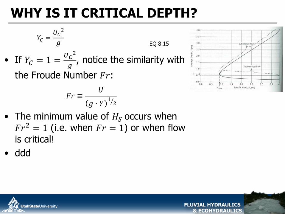
WHY IS IT CRITICAL DEPTH?

• If 𝑌𝐶 = 1 =𝑈𝐶2

𝑔, notice the similarity with

the Froude Number 𝐹𝑟:

• The minimum value of 𝐻𝑆 occurs when 𝐹𝑟2 = 1 (i.e. when 𝐹𝑟 = 1) or when flow is critical!

• ddd

𝑌𝐶 =𝑈𝐶2

𝑔 EQ 8.15

𝐹𝑟 ≡𝑈

𝑔 ∙ 𝑌 12

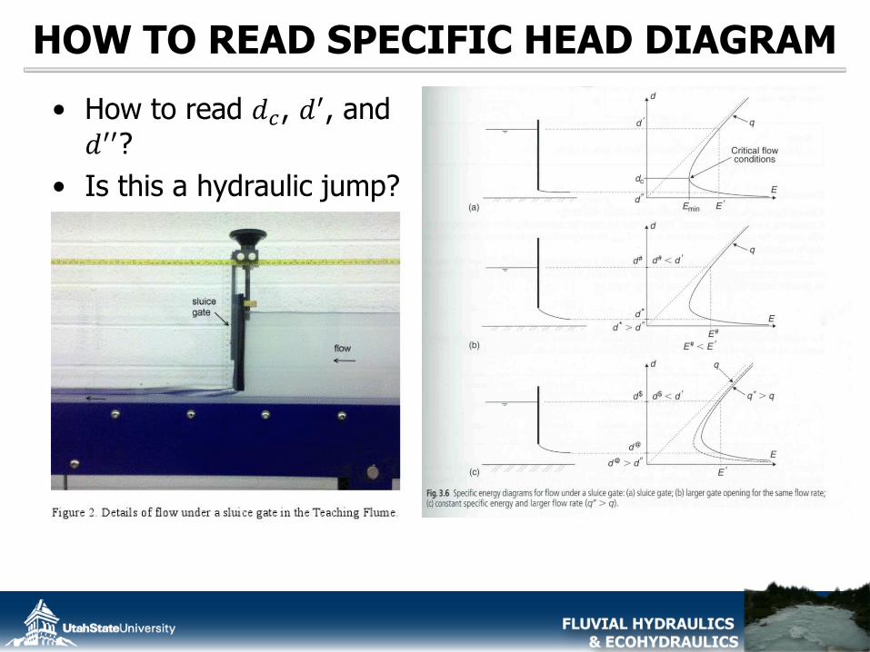
HOW TO READ SPECIFIC HEAD DIAGRAM

• How to read 𝑑𝑐, 𝑑′, and

𝑑′′?

• Is this a hydraulic jump?

TODAY’S PLAN B

I. Energy Principle in 1D Flows

I. The Energy Equation (§ 8.1.1)

II. Specific Energy (§ 8.1.2)

ENERGY & MOMENTUM PRINCIPLES (Applied to 1D flows)

From Dingman (2008), Chapter 8

THIS WEEK’S LAB

• We will do a complete lab assignment and calculations for a hydraulic jump produced by a sluice gate

• You’ll get to put the energy equation to use

• We will then play with different configurations of the flume to induce different hydraulics. We will play with:

– Width constrictions

– Different spillways

– Altering Q & S