Water Vapour Imagery and Potential Vorticity
60
Water Vapour Imagery and Potential Vorticity
description
Water Vapour Imagery and Potential Vorticity. Questions. How can you visualize the wind? How can you see the upper air flow? What colour is the wind?. OUTLINE. Some Physics Imagery Characteristics WV Interpretation NWP Verification Potential Vorticity – Introduction PV Anomalies - PowerPoint PPT Presentation
Transcript of Water Vapour Imagery and Potential Vorticity
Water Vapour Imagery and
Potential Vorticity
Questions
• How can you visualize the wind?
• How can you see the upper air flow?
• What colour is the wind?

OUTLINE Some Physics Imagery Characteristics WV Interpretation NWP Verification Potential Vorticity – Introduction PV Anomalies PV and WV Imagery
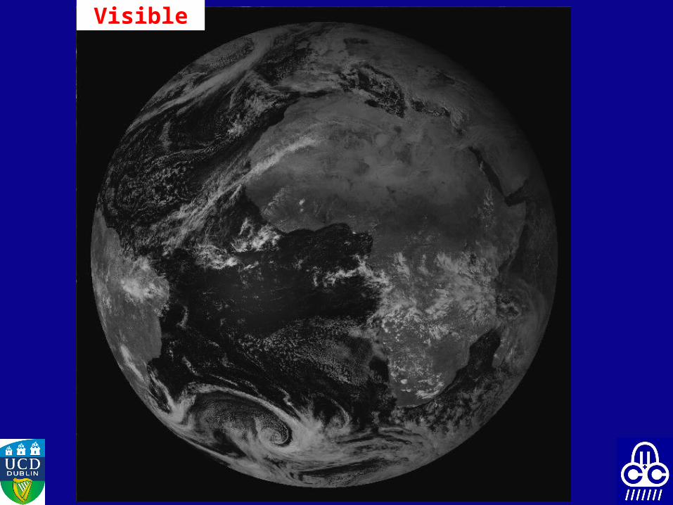
Visible
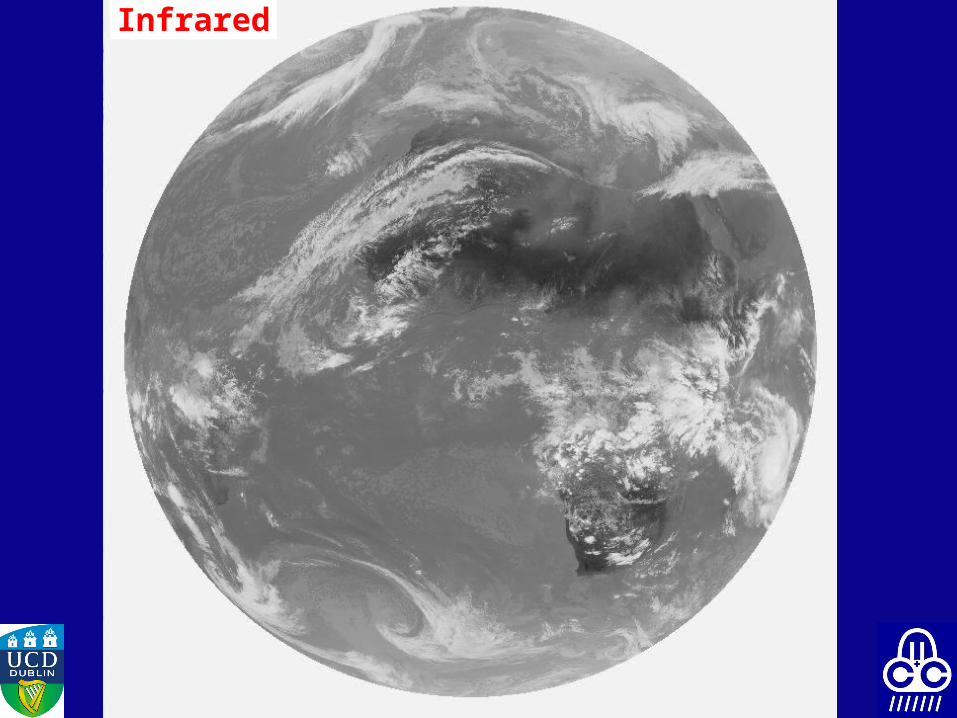
Infrared

Water Vapour
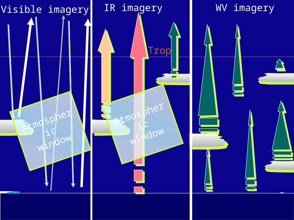
Visible imagery IR imagery WV imagery
Trop
Atmospher
ic
window
Atmospher
ic
window
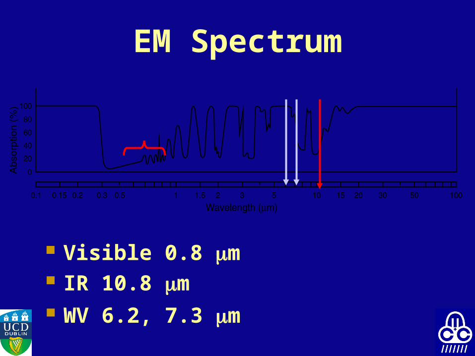
EM Spectrum
Visible 0.8 m IR 10.8 m WV 6.2, 7.3 m

Distribution of WV
Emitting water molecules
Completely moist atmosphereCompletely moist atmosphere

Distribution of WV
Emitting water molecules
Completely moist atmosphereCompletely moist atmosphere
Where is the source of radiation detected at the satellite?
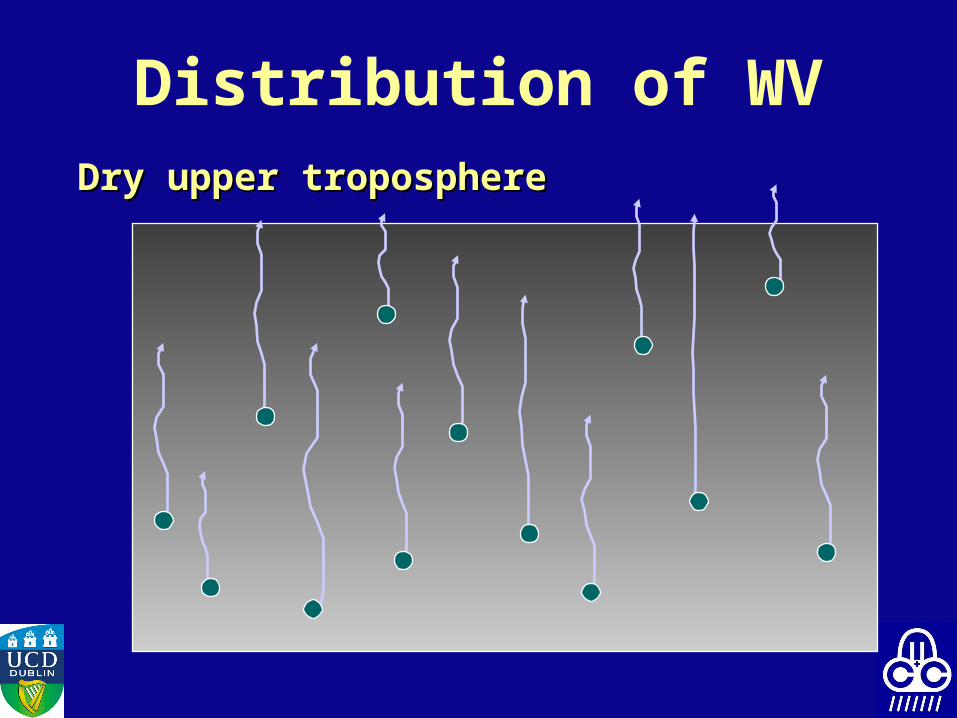
Dry upper troposphereDry upper troposphere
Distribution of WV
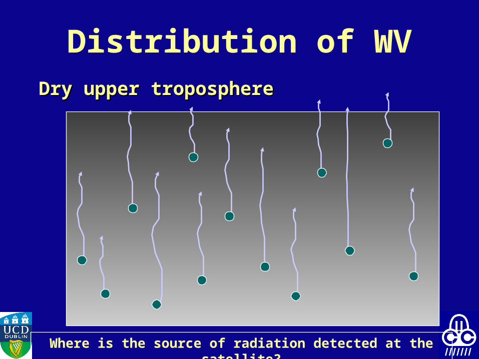
Dry upper troposphereDry upper troposphere
Where is the source of radiation detected at the satellite?
Distribution of WV

Moisture profiles and radiation
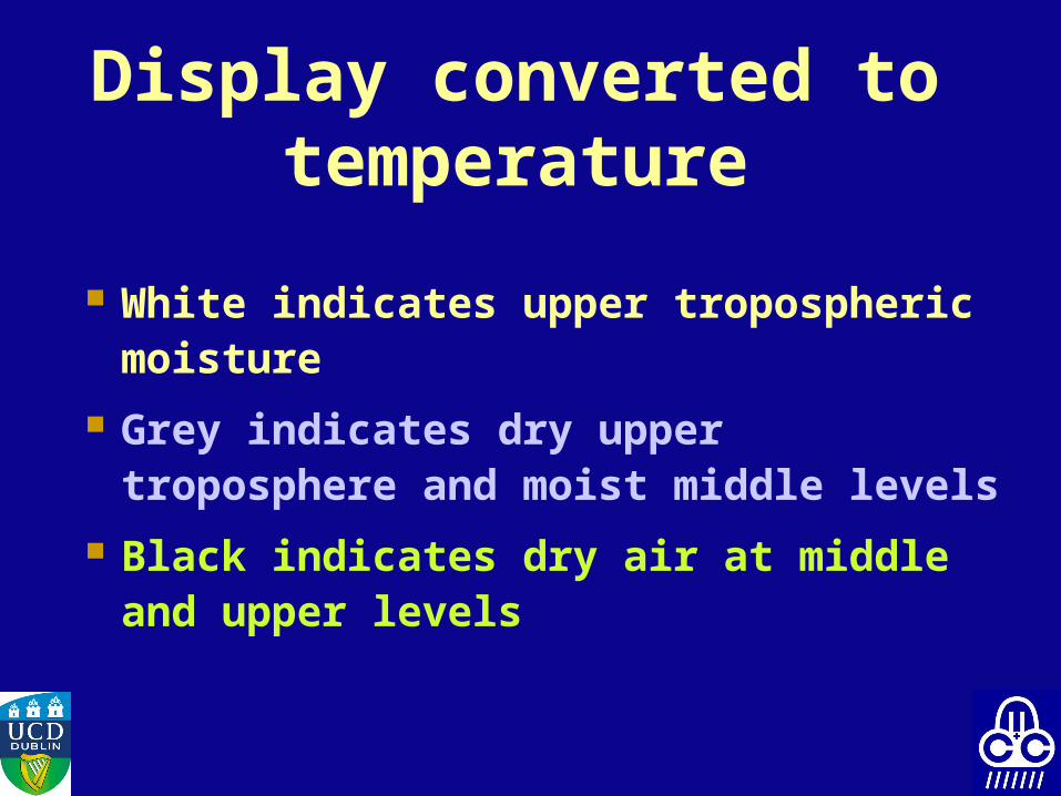
Display converted to temperature
White indicates upper tropospheric moisture
Grey indicates dry upper troposphere and moist middle levels
Black indicates dry air at middle and upper levels
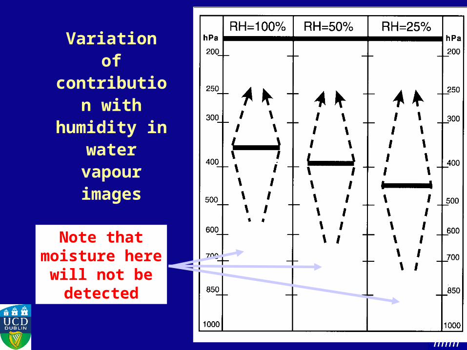
Variation of contributio
n with humidity in
water vapour images
Note that moisture
herewill not be detected

EM Spectrum
Channel 5 (6.2m) strong absorption, centred around 300 hPa
Channel 6 (7.3m) less strong absorption, centred near 500 hPa
WV imagery characteristics
Water vapour loop6-8 June, 2000

1. Latitude Effect Whiter at the poles
– Moisture from colder source Higher contrast in tropics
– Can be cold or warm– More moisture variability– Higher tropopause– Moist air appears dark when it is warm

1. Latitude Effect1. Latitude Effect
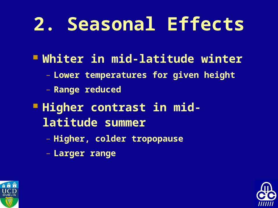
2. Seasonal Effects Whiter in mid-latitude winter
– Lower temperatures for given height– Range reduced
Higher contrast in mid-latitude summer– Higher, colder tropopause– Larger range

2. Seasonal EffectsWinter

2. Seasonal Effects2. Seasonal EffectsSummer

3. Crossover effect All radiation detected
from 700-200hPa A given intensity may
come from different profiles
It’s been found that …– cloud at mid levels
contributes more radiation than higher levels

Imagery interpretation
Broadscale upper flow patterns– Jetstreams– Troughs/Ridges
Areas of vertical motion Short-wave features Convection


6060
30
60
60
60
30
0
0
30
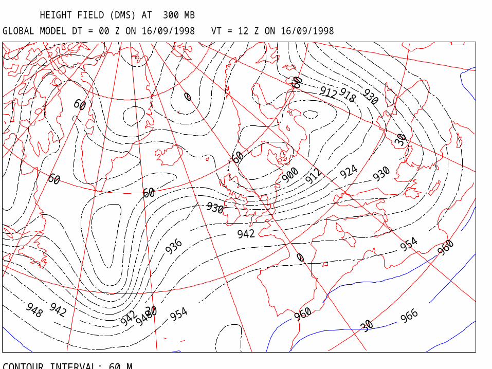
HEIGHT FIELD (DMS) AT 300 MB GLOBAL MODEL DT = 00 Z ON 16/09/1998 VT = 12 Z ON 16/09/1998
912918 930
900
912 924
930
930
936 942954
960
948 942942948 954 960 966
CONTOUR INTERVAL: 60 M

6060
30
60
60
60
30
0
0
30
HEIGHT FIELD (DMS) AT 300 MB GLOBAL MODEL DT = 00 Z ON 16/09/1998 VT = 12 Z ON 16/09/1998
912918 930
900
912 924
930
930
936 942954
960
948 942942948 954 960 966
CONTOUR INTERVAL: 60 M

Water Vapour and NWP
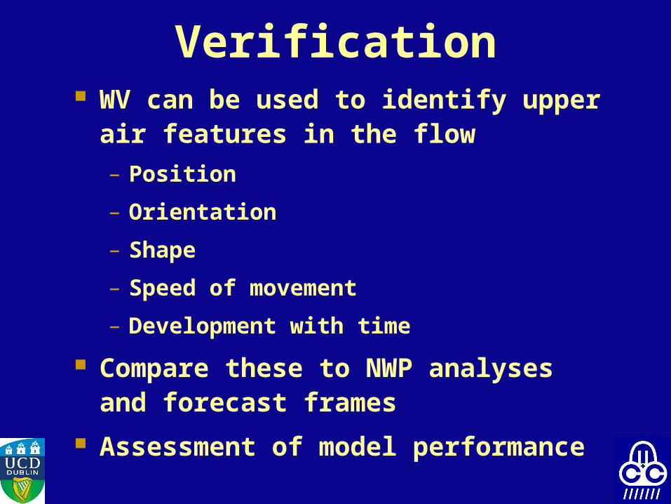
Verification WV can be used to identify upper
air features in the flow– Position– Orientation– Shape– Speed of movement– Development with time
Compare these to NWP analyses and forecast frames
Assessment of model performance
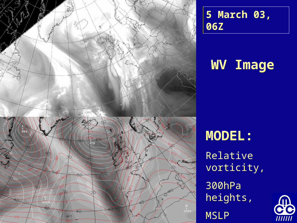
5 March 03, 06Z
MODEL:Relative vorticity,
300hPa heights,
MSLP
WV Image

Recapitulation on WV
Water vapour imagery … shows upper level flows and humidity
patterns in cloud-free areas can be directly compared to model
fields (height, vorticity, vertical motion) can show developments before cloud
formation is evident on VIS/IR

Any Questions(so far)?

Potential Vorticity
A refresher!
Objectives to write down the equation for PV and
understand the meaning of the terms
to describe the effects of a PV anomaly on atmospheric development
to describe how PV can be related to water vapour imagery and NWP

Potential Vorticity PV simply combines vorticity
and static stability (vertical temperature gradient).
P = 1 a. z
density absolutevorticity
vertical potentialtemperaturegradient
How does PV vary? Density decreases with height so PV
tends to increase slightly upwards. f, the Coriolis parameter increases
with latitude, so PV increases slightly towards the poles.
The major change in PV occurs at the tropopause where the static stability increases very rapidly.

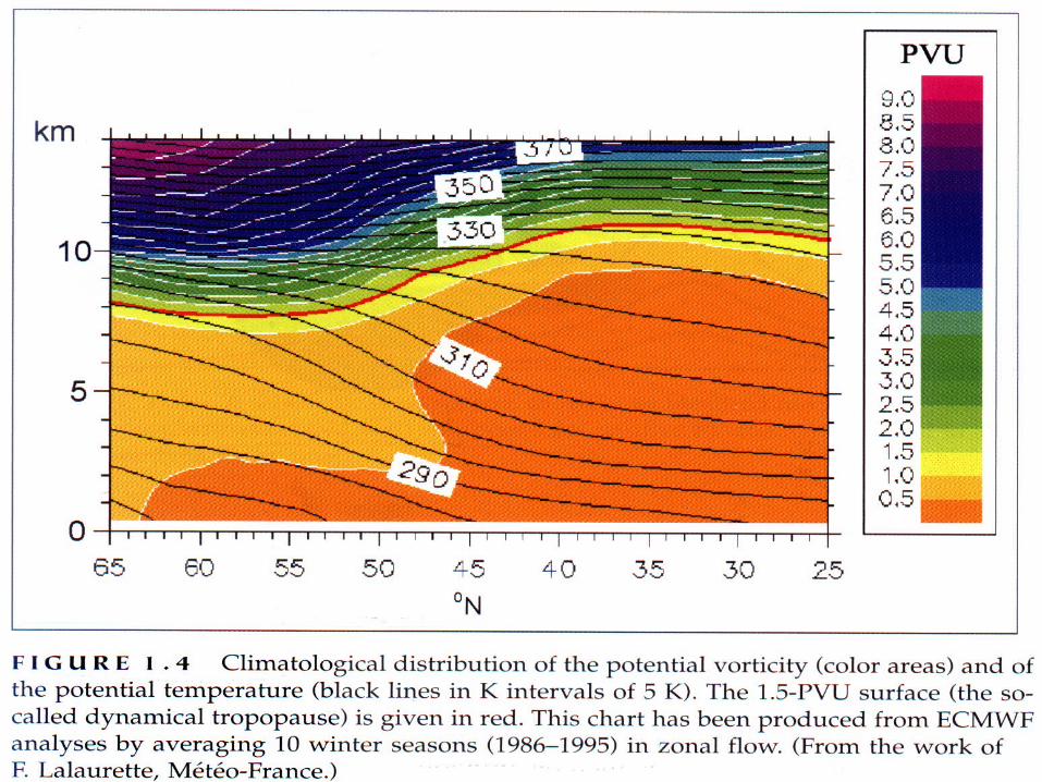
How does PV vary? Typical values of PV in the
troposphere are generally less than 1.5 “PV units”.
In the stratosphere PV increases rapidly to in excess of 4 “PV units”.
Therefore there is a large gradient of PV at the tropopause
(1 PV unit = 10-6 m2s-1 K.kg-1)
Potential Vorticity
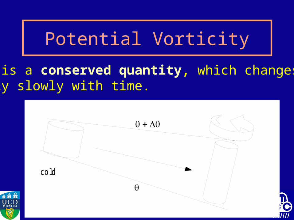
PV is a conserved quantity, which changesonly slowly with time.
co ld
Potential Vorticity This fits with what we already
know about vorticity If we stretch a column of air it
spins more rapidly If we squash an air column it
spins less rapidly

Invertibility PV contains information about both
the dynamics (through vorticity) and thermodynamics (through potential temperature) of the atmosphere.
This is enough information to give all the other atmospheric fields if we have a boundary condition and a balance state.
Invertibility So if you know the PV distribution
in the atmosphere together with say the MSLP field, you can get all the other fields.
You could write an NWP model using PV and it would be cheaper to run than a conventional model.
PV Anomalies
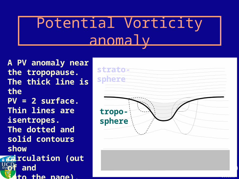
Potential Vorticity anomaly
A PV anomaly near the tropopause.The thick line is thePV = 2 surface.Thin lines areisentropes.The dotted and solid contours showcirculation (out of andinto the page).
strato-sphere
tropo-sphere

The effect of a Potential Vorticity anomaly
strato-sphere
tropo-sphere
A column of air passing beneath thePV anomaly isstretched and so gains some cyclonicvorticity.
In reality the upperlevel features movefaster than low levelair.

The effect of a Potential Vorticity anomaly
An upper level PV anomaly induces low level vorticity.
Upper level PV anomalies occur where the tropopause changes height rapidly.
Tropopause height changes rapidly in the vicinity of fronts, developing depressions, upper lows or cold pools.

An upper low / cold pool
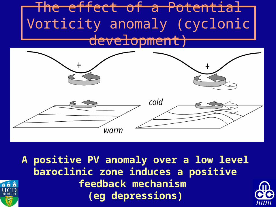
The effect of a Potential Vorticity anomaly (cyclonic development)
+ +
warm
cold
A positive PV anomaly over a low level baroclinic zone induces a positive feedback mechanism
(eg depressions)

Potential Vorticity anomalies
00Z 2/11/92. PV (colours). 900 hPa w (white) MSLP (black)

Potential Vorticity anomalies
00Z 3/11/92 (24 hours later) PV (colours). 900 hPa w (white) MSLP (black)

PV and WV Imagery

PV and water vapour imagery
Stratospheric air has high PV and low humidity.
The upper troposphere in a tropical airmass has low PV and high humidity.
In mid latitudes PV values near the tropopause relate closely to radiances in the water vapour channel.
PV and water vapour imagery
In a developing depression, the tropical air in the warm conveyor belt will be white or pale grey in a WV image, and will have low PV.
The dry, cold descending air behind the system will be dark grey or black in a WV image and will have high PV.
Where the tropopause is changing height rapidly, there will be a sharp PV gradient.

PV and water vapour imagery
PV and water vapour imagery
This means that the PV field from an NWP model is almost like a forecast water vapour image.
If the PV distribution from the model is overlaid on a water vapour image, the quality of the analysis or forecast can be subjectively assessed.
PV and water vapour imagery
The model’s PV field at T+0 can be compared with water vapour imagery.
If they do not match well, the model analysis can be adjusted to give a better fit and therefore a better forecast.
This provides a means of evaluating and improving NWP forecasts.

Any Questions?