Water, salt, and heat budget

Conservation laws

application: box models

Surface fresh water flux:

evaporation, precipitation, and river runoff

Surface heat flux components:

sensible, latent, long and shortwave

Ocean meridional transport

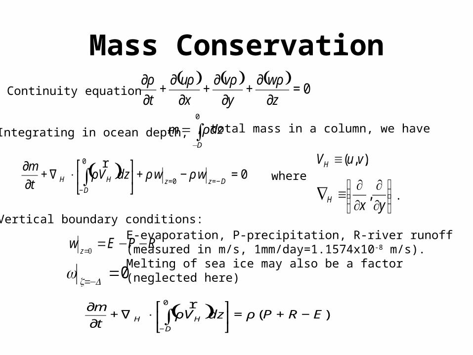
Mass Conservation

Continuity equation

( ) ( ) ( )0=

∂

∂+

∂

∂+

∂

∂+

∂

∂

z

w

y

v

x

u

t

ρρρρ

Mass Conservation( ) ( ) ( )

0=∂

∂+

∂

∂+

∂

∂+

∂

∂

z

w

y

v

x

u

t

ρρρρContinuity equation

Integrating in ocean depth, ∫−

=0

D

dzm ρ , total mass in a column, we have

( ) 00

0

=−+⎥⎦

⎤⎢⎣

⎡⋅∇+

∂

∂−==

−∫ DzzD

HH wwdzVt

mρρρ

r

. ⎟⎟⎠

⎞⎜⎜⎝

⎛∂∂

∂∂

≡∇yxH ,

, ),( vuVH ≡

RPEwz

−−==0

E-evaporation, P-precipitation, R-river runoff (measured in m/s, 1mm/day=1.1574x10-8 m/s).Melting of sea ice may also be a factor(neglected here)

where

Vertical boundary conditions:

0=−= Dz

w

( ) )(0

ERPdzVt

m

D

HH −+=⎥⎦

⎤⎢⎣

⎡⋅∇+

∂

∂∫

−

ρρr

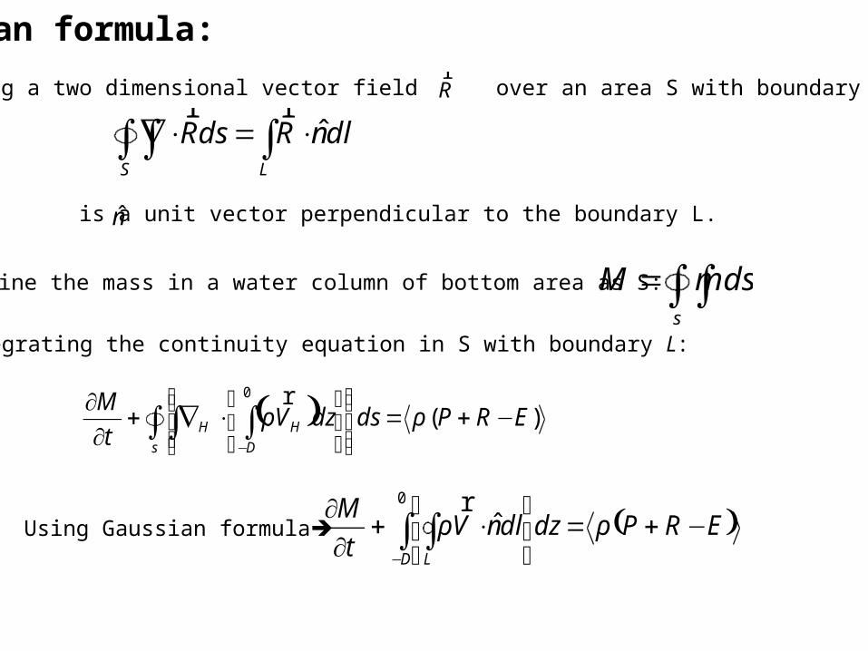
Integrating the continuity equation in S with boundary L:

∫∫=s

mdsM

( )∫∫ ∫ −+=⎪⎭

⎪⎬⎫

⎪⎩

⎪⎨⎧

⎥⎦

⎤⎢⎣

⎡⋅∇+

∂∂

−s D

HH ERPdsdzVt

M)(

0

ρρr

( )∫∫−

−+=⎥⎦

⎤⎢⎣

⎡⋅+

∂∂ 0

ˆD L

ERPdzdlnVt

Mρρ

r

n̂Where is a unit vector perpendicular to the boundary L.

Gaussian formula:

Integrating a two dimensional vector field over an area S with boundary L, we have

Define the mass in a water column of bottom area as S:

Using Gaussian formula

∫∫ ∫ ⋅=⋅∇S L

dlnRdsR ˆrr

Rr

0=Vr

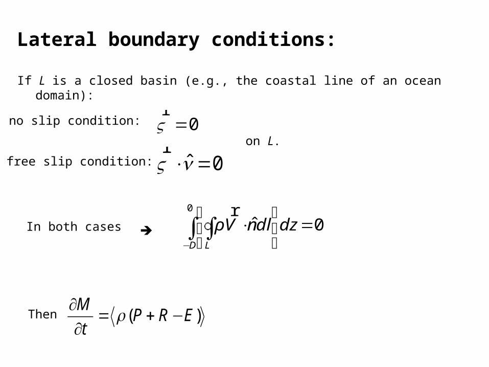
free slip condition: 0ˆ =⋅nVr on L.

∫∫−

=⎥⎦

⎤⎢⎣

⎡⋅

0

0ˆD L

dzdlnVr

ρ

)( ERPt

M−+=

∂∂ ρ

Lateral boundary conditions:

If L is a closed basin (e.g., the coastal line of an ocean domain):

no slip condition:

In both cases

Then

Salt Conservation

€ ∂ρS()∂t+∂uρS()∂x+∂vρS()∂y+∂wρS()∂z=ρκS∇32S€ ∇32S=∂2S∂x2+∂2S∂y2+∂2S∂z2where

smS29105.1 −×≈κ Molecular diffusivity of salt

€ ρuS=ρuS=ρu +′ u ()S +′ S ()=ρu S +ρ′ u ′ S

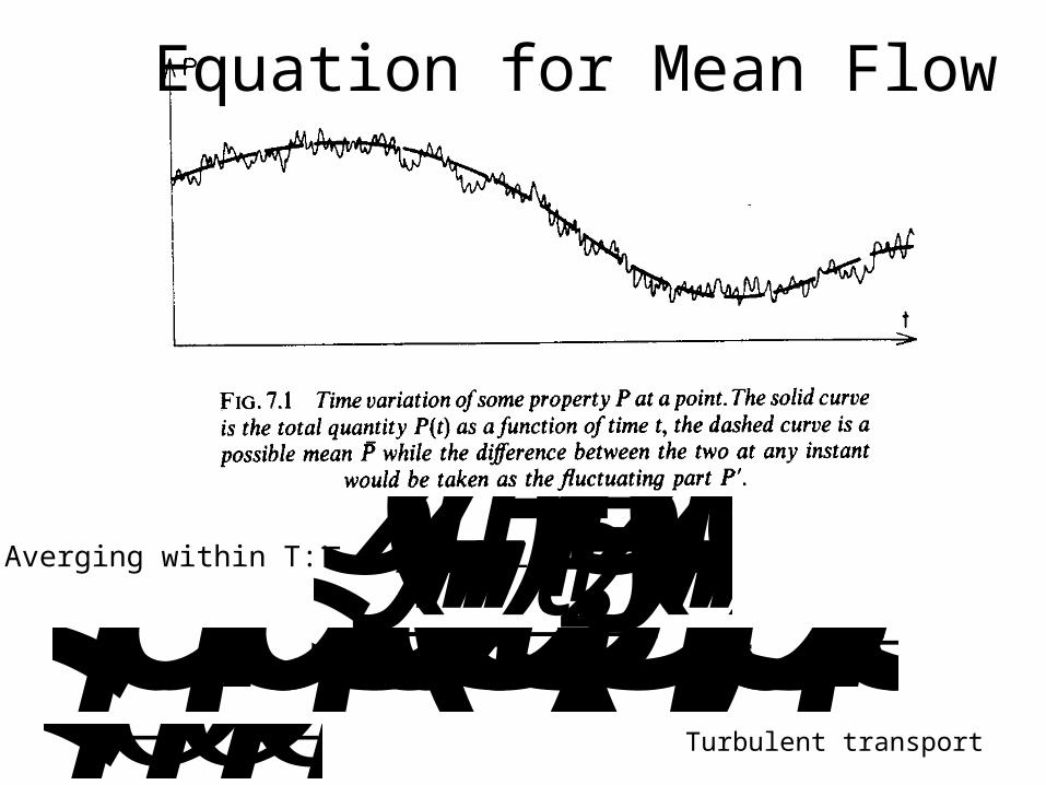
Equation for Mean Flow

Averging within T:

€ S x,y,z,t,T( )=1TSx,y,z,′ t ()d′ t t−T2

t+T2∫Turbulent transport€ ρ=ρ +′ ρ ≈ρ

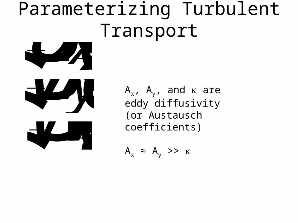
Parameterizing Turbulent Transport

€ ′ u ′ S =−Ax∂S ∂x

€ ′ v ′ S =−Ay∂S ∂y

€ ′ w ′ S =−κ∂S ∂z

Ax, Ay, and κ are eddy diffusivity (or Austausch coefficients)

Ax ≈ Ay >> κ

Salt Conservation ( ) ( ) ( ) ( ) ( ) ⎟

⎠

⎞⎜⎝

⎛∂∂

∂∂

+∇⋅∇=∂

∂+

∂∂

+∂

∂+

∂∂

z

S

zSA

z

Sw

y

Sv

x

Su

t

SHH ρκρ

ρρρρ

sm234 10~10 −−=κ , vertical eddy diffusion coefficient.

smA 231 10~10−= , horizontal eddy diffusion coefficient.

smS29105.1 −×≈κ The molecular diffusivity of salt is

Ratio between eddy and molecular diffusivity: 610~Sκκ

Integrating for the whole ocean column,

( )[ ]000 =

−=−−

⎟⎠

⎞⎜⎝

⎛∂

∂+−=⎟⎟

⎠

⎞⎜⎜⎝

⎛∇−⋅∇+⎟⎟

⎠

⎞⎜⎜⎝

⎛

∂

∂∫∫

z

DzD

HHH

D z

SSwdzSASVSdz

tρκρρρ

r

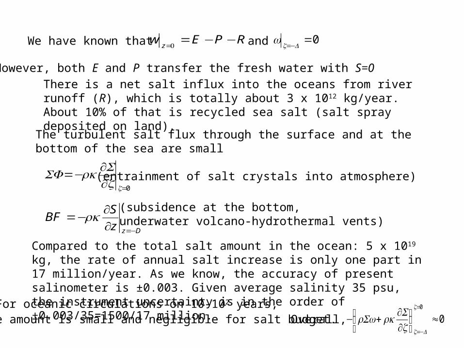
RPEwz

−−==0We have known that 0=

−= Dzwand

However, both E and P transfer the fresh water with S=0

There is a net salt influx into the oceans from river runoff (R), which is totally about 3 x 1012 kg/year. About 10% of that is recycled sea salt (salt spray deposited on land).

0=∂∂

−=zz

SSF ρκ

The turbulent salt flux through the surface and at the bottom of the sea are small

Dzz

SBF

−=∂∂

−= ρκ

(entrainment of salt crystals into atmosphere)

the amount is small and negligible for salt budget.

(subsidence at the bottom, underwater volcano-hydrothermal vents)

00

≈⎟⎠

⎞⎜⎝

⎛∂∂

+−=

−=

z

DzzS

Sw ρκρOverall,

Compared to the total salt amount in the ocean: 5 x 1019 kg, the rate of annual salt increase is only one part in 17 million/year. As we know, the accuracy of present salinometer is ±0.003. Given average salinity 35 psu, the instrument uncertainty is in the order of ±0.003/35=1500/17 million.

For oceanic circulations on 10-102 years,

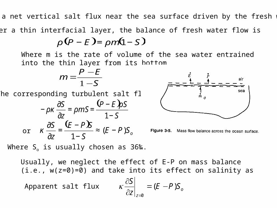
There is a net vertical salt flux near the sea surface driven by the fresh water flux.

Consider a thin interfacial layer, the balance of fresh water flow is

( ) ( )SmEP −=− 1ρρ

Where m is the rate of volume of the sea water entrained into the thin layer from its bottom

S

EPm

−−

=1

The corresponding turbulent salt flux is

( )S

SEPmS

z

S

−

−==

∂

∂−

1

ρρρκ

( )oSPE

S

SPE

z

S)(

1−≈

−

−=

∂

∂κor

Where So is usually chosen as 36‰.

Usually, we neglect the effect of E-P on mass balance (i.e., w(z=0)=0) and take into its effect on salinity as

oz

SPEz

S)(

0

−=∂∂

=

κApparent salt flux

Box ModelUnder steady-state conditions, we apply the conservations of mass and salt to a box of volume V filled with sea water.

Conservation of volume:

Where Vi is inflow, Vo outflow; P precipitation, E evaporation, and R river runoff.

EVPRV oi +=++

Salt conservation: oooiii SVSV ρρ =influx outflux

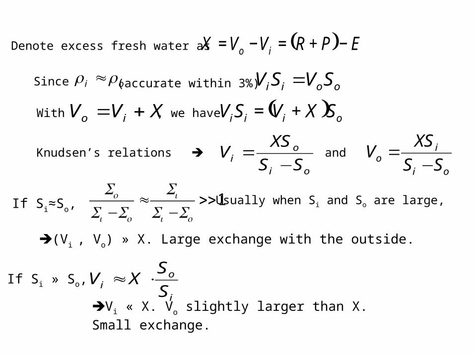
Denote excess fresh water as ( ) EPRVVX io −+=−=

oi ρρ ≈

XVV io +=

Since

With , we have ( ) oiii SXVSV +=

oi

oi SS

XSV

−=

oi

io SS

XSV

−=

1>>−

≈− oi

i

oi

o

SSS

SSS

i

oi S

SXV ⋅≈

ooii SVSV =

and

If Si≈So,

(Vi , Vo) » X. Large exchange with the outside.

If Si » So,

Vi « X. Vo slightly larger than X. Small exchange.

Knudsen’s relations

Usually when Si and So are large,

(accurate within 3%)

Basin Mediterranean Sea Black Sea

Totoal volume (km3) 3.8 x 1060.6 x 106

X=P-E(m3/s) -7x104 6.5 x 103

Si 36.3 35

So 37.8 17

Vi (m3/s, km3/yr) 1.75x106, 5.5 x 104 6x103, 0.02x104

Vo(m3/s) 1.68 x 106 13x103

Flushing time (yr) 70 3000

Examples

Circulation Patterns

O2 > 160 mol/kg (4ml/l)

Hydrogen SulphideH2S~6ml/l

Annual Mean Precipitation (mm/day)-COADS

Annual mean evaporation (mm/day)-COADS

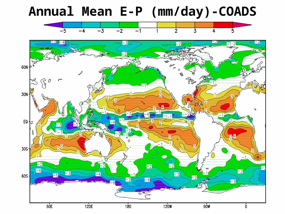
Annual Mean E-P (mm/day)-COADS

An evaporation rate of 1.2 m/yr is equivalent to removing about 0.03% of the total ocean volume each year. An equivalent amount returns to the ocean each year, about 10% by way of rivers and the remainder by rainfall.

The yearly salt exchange is less than 10-7 of the total salt content of the ocean.

Wijffels, 2001

Where transport increases northward, freshwater is being added to the ocean.

Freshwater added80oS-40oS10oS-10oN40oN-80oN

Freshwater removed40oS-10oS10oN-40oN

Transport should be zero at the poles for global balance

The fresh water transport is small compared to the total circulation