Water-Resources Investigations Report 85-4210

COST EFFECTIVENESS OF THE STREAM-GAGING PROGRAM IN SOUTH CAROLINA

By A. Carroll Barker, Benjamin C. Wright, and Curtis S. Bennett III

U.S. GEOLOGICAL SURVEY

Water-Resources Investigations Report 85-4210

Columbia, South Carolina

1985

UNITED STATES DEPARTMENT OF THE INTERIOR

DONALD PAUL MODEL, Secretary

GEOLOGICAL SURVEY

Dallas L. Peck, Director

For additional information write to:

District Chief U.S. Geological Survey, WRD 1835 Assembly Street, Suite 658 Columbia, South Carolina 29201

Copies of this report can be purchased from*

Open-File Services Section Western Distribution Branch Box 25425, Federal Center Denver, Colorado 80225 (Telephone» 303/236-7476)

CONTENTS

PageAbstract ............................... 1

Introduction ............................. 2

History of the stream-gaging program in South Carolina ...... 3Current South Carolina stream-gaging program ........... 5

Uses, funding, and availability of continuous streamflow data. .... 11

Data-use classes ......................... 11Regional hydrology. ..................... 11Hydrologic systems. ..................... 11Planning and design ..................... 12Project operation ...................... 12Hydrologic forecasts. .................... 12Water-quality monitoring. .................. 12Research. .......................... 25

Funding. ............................... 25Frequency of data availability .................... 25Data-use presentation. ........................ 26Conclusions pertaining to data uses. ................. 26

Alternative methods of developing streamflow information ....... 26

Flow-routing model ........................ 27-28Regression analysis. ....................... 29Categorization of stream gages by their potential for alternative

methods. ............................ 30Richtex flow-routing analysis. ................ 31-33Branchville flow-routing analysis. .............. 34-36Regression analysis results. ................. 38-40Conclusions pertaining to alternative methods of data generation 40

Cost-effective resource allocation .................. 41

Kalman-filtering method for cost-effective resource. .......allocation (K-CERA). ...................... 41

Description of mathematical program. ............... 41-45Description of uncertainty functions ............... 45-49The application of K-CERA in South Carolina. ........... 49

Definition of missing record probabilities. ......... 50Definition of cross-correlation coefficient and coefficient

of variation. ....................... 51Kalman-filter definition of variance. ............ 51-54

Determination of routes and costs. ................ 59K-CERA results. ....................... 65

Conclusions from the K-CERA analysis ............... 74

111

CONTENTS (Continued)

Page Summary. ............................... 75

References cited ........................... 76-77

ILLUSTRATIONS

Figure 1. Graph showing history of continuous stream gaging inSouth Carolina. ..................... 4

2. Map showing location nf stream-gaging stations in thephysiographic provinces of South Carolina ........ 6

3. Map showing location of stations for other than stream gagingonly. .......................... 7

4. Daily hydrograph, Edisto River near Branchville, winter1982. .......................... 37

5. Tabular form of optimization of routing of hydrographers. . 44

6-9. Graphs showing

6. Autocovariance function for station 02160700 ..... 55

7. Autocovariance function for station 02171630 ..... 55

8. Typical uncertainty function for instantaneousdischarge. ...................... 56

9. Average standard error per stream gage ........ 66

IV

CONTENTS (Continued)

TABLES

Page Table 1. Selected hydrologic data for stations in the South Carolina

stream-gaging program. .................. 8-10

2. Use of data from stream-gaging stations in South Carolina. . 13-24

3. Gaging stations used in the Richtex flow-routing analysis. . 31

4. Selected reach characteristics used in the Richtex flow- routing analysis ..................... 32

5. Simulation errors of the routing model for Richtex flow- routing analysis ..................... 33

6. Gaging stations used in the Branchville flow-routinganalysis ......................... 34

7. Selected reach characteristics used in the Branchville flow- routing analysis ..................... 35

8. Simulation errors of the routing model for Branchville flow- routing analysis ..................... 36

9. Summary of calibration for regression modeling of daily meanstreamflow at selected stations in South Carolina. .... 39

10. Statistics of record reconstruction. ............ 52-53

11. Summary of the autocovariance analysis ........... 57-58

12. Summary of the routes that may be used to visit stations inSouth Carolina ...................... 60-64

13. Selected results of K-CERA analysis. ............ 67-73

CONVERSION FACTORS AND ABBREVIATIONS OF UNITS

The following factors may be used to convert the inch-pound units published herein to the International System of units (SI).

Multiply inch-pound units

foot (ft)

mile (mi)

square mile (mi^)

cubic foot (ft3 )

foot per second (ft/s)

cubic foot per second (ft3/s)

Length

0.3048

1.609

Area

2.590

Volume

Flow

0.3048

0.02832

To obtain SI units

meter (m)

kilometer (km)

square kilometer (km2)

0.02832 cubic meter (m3 )

meter per second (m/s)

cubic meter per second (m3/s)

VI

COST EFFECTIVENESS OF THE STREAM-GAGING PROGRAM IN SOUTH CAROLINA

By A. Carroll Barker, Benjamin C. Wright, and Curtis S. Bennett III

ABSTRACT

This report documents the cost effectiveness of the stream-gaging program in South Carolina for the 1983 water year. Data uses and funding sources were identified for the 76 continuous stream gages currently being operated in South Carolina. The budget of $422,200 for collecting and analyzing streamflow data also includes the cost of operating stage-only and crest-stage stations. The streamflow records for one stream gage can be determined by alternate, less costly methods, and should be discontinued. The remaining 75 stations should be maintained in the program for the foreseeable future.

The current policy for the operation of the 75 stations including the crest-stage and stage-only stations would require a budget of $417,200 per year. The average standard error of estimation of streamflow records is 16.9 percent for the present budget with missing record included. However, the standard error of estimation would decrease to 8.5 percent if complete streamflow records could be obtained. It was shown that the average standard error of estimation of 16.9 percent could be obtained at the 75 sites with a budget of approximately $395,000 if the gaging resources were redistributed among the gages.

A minimum budget of $383,500 is required to operate the program; a budget less than this does not permit proper service and maintenance of the gages and recorders. At the minimum budget, the average standard error is 18.6 percent. The maximum budget analyzed was $850,000, which resulted in an average standard error of 7.6 percent.

INTRODUCTION

The U.S. Geological Survey is the principal Federal agency collecting streamflow data in the nation. The collection of these data is a major activity of the Water Resources Division of the U.S. Geological Survey. The data are collected in cooperation with State and local governments and other Federal agencies. The U.S. Geological Survey is presently (1985) operating approximately 8,000 continuous-record gaging stations throughout the nation. Some of these records extend back to the turn of the century. Any activity of long standing, such as the collection of streamflow data, should be reexamined at intervals, if not continuously, because of changes in objectives, technology, or external constraints. The most recent systematic nationwide evaluation of the stream-gaging program was completed in 1970 (Benson and Carter, 1973). The U.S. Geological Survey is presently undertaking another nationwide analysis of the stream-gaging program that will be completed over a 5-year period with 20 percent of the program being analyzed each year.

The objective of this analysis is to define and document the most cost- effective means of furnishing streamflow information for South Carolina. For every continuous-record gaging station, the analysis identifies the principal uses of the data and relates these uses to funding sources. Stations for which data are no longer needed are identified, as are deficient or unmet data demands. In addition, gaging stations are categorized as to whether the data are available to users in a real-time sense, on a provisional basis, or at the end of the water year.

The second aspect of the analysis is to identify less costly alternate methods of furnishing the needed information; among these are flow-routing models and statistical methods. The stream-gaging program no longer is considered a network of observation points, but rather an integrated information system in which data are provided by both observation and synthesis.

The final part of the analysis involves the use of Kalman-filtering and mathematical-programming techniques to define strategies for operation of the necessary stations that minimize the uncertainty in the streamflow records for given operating budgets. Kalman-filtering techniques are used to compute uncertainty functions relating the standard errors of computation or estimation of streamflow records to the frequencies of visits to the stream gages for all stations in the analysis. A steepest-descent optimization program uses these uncertainty functions, information on practical stream-gaging routes, the various costs associated with stream gaging, and the total operating budget to identify the visit frequency for each station that minimizes the overall uncertainty in the computation of streamflow. The stream-gaging program that results from this analysis will meet the expressed water-data needs in the most cost-effective manner.

This report is organized into five sections; the first section is an introduction to the stream-gaging activities in South Carolina and to the study itself. The middle three sections each contain discussions of an individual step of the analysis. Because of the sequential nature of the steps and the dependence of subsequent steps on the previous results, summaries of conclusions are given at the end of each of the middle three sections. The complete study is summarized in the final section.

History of the Stream-Gaging Program in South Carolina

The program of streamflow investigations by the U.S. Geological Survey in South Carolina has grown rather steadily through the years as Federal and State interest in water resources has increased (fig. 1). Streamflow records have been obtained in South Carolina by the U.S. Geological Survey since 1883, when a gaging station providing a daily discharge record was established on the Savannah River near Augusta, Georgia. River stages had been collected and published by the U.S. Weather Bureau as early as 1875 at the same site. In 1900, discharge records were collected at two stations in the State, and the program remained at this level until 1906. Between 1906 and 1930 the number of stations fluctuated from 0 in 1910 to 14 in 1930. Collection of these streamflow records was the responsibility of the U.S. Geological Survey's office in Asheville, North Carolina.

On November 1, 1930, the South Carolina District WRD of the U.S. Geological Survey Cooperative programs were begun with the South Carolina State Highway Department (now the South Carolina Department of Highways and Public Transportation), several Federal Power Commission licensees, and the U.S. Army Corps of Engineers. Three new gaging stations were constructed in 1934 through a cooperative agreement with the Soil Erosion Service (now the Soil Conservation Service) of the U.S. Department of Agriculture. Six additional gaging stations were established in 1938 at the request of the U.S. Army Corps of Engineers. By 1951, the South Carolina District operated 55 gaging stations and in 1969 there were 64 stations.

The formation of the South Carolina Research, Planning and Development Board in 1946 (now the South Carolina State Development Board) established a low-flow partial record program. The network provided low-flow data at sites that were not gaged regularly, but were considered as potential industrial locations.

The data collection program was further expanded in 1966 to investigate flood frequencies on small streams for the South Carolina Department of Highways and Public Transportation. The network consisted of 56 partial- record stations that were equipped with dual digital stage-rainfall recorders.

Carter and Benson (1970) proposed an approach for evaluating stream- gaging programs. A study by Armbruster (1970) described the development of the South Carolina stream-gaging program needed to meet the needs of future water-data users. There were 64 stations at the time of the study. Eleven stations were discontinued and one station was added after the study was completed. Between 1970 and 1983, 27 stations were added and 15 were eliminated from the South Carolina stream-gaging program. Currently, there are 76 continuous stream gages in operation in South Carolina.

CQ C

t-J CD I

(0 o

o

o

o D n- C

O C O)

rf

(Q

CD

CQ (Q CO

O c

m rn en

(0 to

o (0 (0

O) o

o CD ED

(O

00

O

NU

MB

ER

OF

CO

NT

INU

OU

S D

AIL

Y

DIS

CH

AR

GE

ST

AT

ION

S S

INC

E 1

900

Current South Carolina Stream-Gaging Program

The locations of the 76 stream gages currently operated by the South Carolina District of the U.S. Geological Survey and their distribution in various physiographic provinces of the state are shown in figure 2. Eighteen gages are located in the lower Coastal Plain, 29 are located in the inner Coastal Plain, 27 are located in the Piedmont, and 2 are located in the Blue Ridge Province. The location of stations for other than continuous stream-gaging only are shown in figure 3.

The cost of operating the 76 stream gages, the 16 stage-only stations, and the 40 crest-stage stations in fiscal year 1983 was $422,200.

Selected hydrologic data, including drainage area, period of record, and mean annual flow for the 76 stations are given in table 1. Station identification numbers used throughout this report are the U.S. Geological Survey eight-digit downstream order station number except in figures 2 and 3, where the first two digits (02) of the standard U.S. Geological Survey station number are omitted. Table 1 also provides the official names and identification numbers of these stations.

:; £

/ V.V V-^i^UTH^ROL/NA^t 295

EX

PL

AN

AT

ION

17

35

00

O

S

UR

FA

CE

WA

TE

R S

TA

TIO

NS

160105

A

RE

GIO

NA

L H

YD

RO

LO

GY

ST

AT

ION

S

\'-<:

-:'-:

\ B

LU

E R

IDG

E P

RO

VIN

CE

(?!

:'1

PIE

DM

ON

T P

RO

VIN

CE

|» '

! C

OA

ST

AL

PL

AIN

PR

OV

INC

E

Figu

re 2

. Lo

cati

on o

f Stream-gaging

stations i

n So

uth

Caro

lina

' '

i-ss

V

-^

. .

.

.\'«

-64

EX

PL

AN

AT

ION

WE

LL

9

CR

ES

T S

TA

GE

GA

GE

«

ST

AG

E O

NL

Y

t

ST

AG

E O

NL

Y &

WA

TE

R Q

UA

LIT

Y

DIS

CH

AR

GE

& W

AT

ER

QU

AL

ITY

I'.1.

1.'.)

{

- '- I

B

LU

E R

IDG

E P

RO

VIN

CE

\'.'

£\i

\ P

IED

MO

NT

PR

OV

INC

E

I- '

-I C

OA

ST

AL

PL

AIN

P

RO

VIN

CE

Figure 3. Loc

atio

n of st

atio

ns for

othe

r th

an stream-gag

ing

only

Table 1. Selected hydrologic data for stations in the South Carolina

Station number

02110500021295900213090002130910021310000213115002131309021314720213200002135000

0213530002135500

0213600002146000

0214700002148000

021483150215378002154500

0215550002156050

021564500215650002157000021601050216070002160775021610000216150002161700

0216201002162093

02162350

stream-gaging program

Station name

Waccamaw River nr LongsWhites Creek nr WallaceBlack Creek nr McBeeBlack Creek nr HartsvillePee Dee River at Pee DeeCatfish Canal at SellersFork Creek at JeffersonHanging Rock Creek nr KershawLynches River at EffinghamLittle Pee Dee River atGalivants Ferry

Scape Ore Swamp nr BishopvilleBlack River nr Gable

Black River at KingstreeCatawba River nr Rock Hill

Catawba River nr CatawbaWateree River nr Camden

Wateree River below EastoverClarks Fork Creek nr SmyrnaNorth Pacolet River at

FingervillePacolet River nr FingervilleLawsons Fork Creek at Dewey

Plant nr InmanNeals Creek nr CarlisleBroad River nr CarlisleNorth Tyger River nr FairmontTyger River nr DeltaEnoree River at WhitmireHellers Creek nr PomariaBroad River at AlstonBroad River at RichtexWest Fork Little River nr

Salem CrossroadsCedar Creek nr BlythewoodSmith Branch at North Main St.

at ColumbiaMiddle Saluda River nrCleveland

Drainage area (mi2 )

1,11026.4108173

8,83027.424.310.1

1,0302,790

96.0401

1,2523,050

3,5305,070

5,59024.1

116

2126.46

12.32,790

44.4759444

8.164,7904,850

25.5

48.95.67

21.0

Period of record

(mo/yr-mo/yr )

03/50-10/79-10/59-10/60-10/38-11/66-10/76-10/80-08/29-10/41-

07/68-06/51-06/6604/72-08/29-09/1895-09/190304/42-10/68-01/03-12/0310/04-09/1010/29-07/63-10/80-10/29-

10/29-10/79-

10/80-10/38-10/50-10/73-10/73-10/80-10/80-10/25-10/80-

11/66-10/76-

10/80-

Mean annual flow (ft3/s)

1,213 *

167236

9,74826.825.4_ *

1,0253,197

107383

9304,567

5,8166,396

_ *_ *

212

354_ *

*

4,05966.2

1,168610 *_ *

6,214--*

48.422.6

_ *

Table 1. Selected hydrologic data for stations in the South Carolinastream- gaging program Continued

Station number

02162525021635000216500002166970021670000216900002169500021695700216963002170500

021715000217156002171650

021716800217264002173000

02173500

0217400002175000021755000217650002176875021852000219625002197000

02197300

02197310

02197315

021973200219732602197330021973320219733402197336

Station name

Hamilton Creek nr EasleySaluda River nr Ware ShoalsReedy River nr Ware ShoalsNinety-Six Creek nr Ninety-SixSaluda River at ChappellsSaluda River nr ColumbiaCongaree River at ColumbiaGills Creek at ColumbiaBig Beaver Creek nr St. Ma thewsLakes Marion-Moultrie Div.Canal nr Pineville

Santee River nr PinevilleSantee River nr RussellvilleSantee River below

St. StephensWedboo Creek nr JamestownDean Swamp Creek nr Sal leySouth Fork Edisto River nrDenmark

North Fork Edisto River atOrangeburg

Edisto River nr BranchvilleEdisto River nr GivhansSalkehatchie River nr MileyCoosawatchie River nr HamptonGreat Swamp nr RidgelandLittle River nr WalhallaHorn Creek nr ColliersSavannah River nr Augusta,

Ga.

Upper Three Runs nr NewEllenton

Upper Three Runs above Road Cat SRP (Savannah River Plant)

Upper Three Runs at Road Aat SRP

Savannah River nr JacksonBeaverdam Creek at 400-D at SRPSite no. 1 at SRPSite no. 2 at SRPSite no. 3 at SRPSite no. 4 at SRP

Drainage area (mi 2 )

1.6058123617.4

1,3602,5207,850

59.610.0

14,70014,80014,900

17.431.2

720

683

1,7202,730

34120348.872.013.9

7,508

87.0

176

203

0.730.130.305.956.96

Period of record

(mo/yr-mo/yr )

10/80-10/38-03/39-10/80-10/26-08/25-10/39-09/66-07/66-10/43-

04/42-10/79-10/70-

09/66-10/80-08/31-09/7110/80-10/38-

10/45-01/39-02/51-02/51-10/78-03/67-10/80-10/1883-12/189101/1896-12/190601/1925-06/66-

06/74-

06/74-01/7810/78-10/71-06/74-08/67-09/67-09/67-08/67-

Mean annual flow (ft3/s)

__*

1,027352__*

1,9742,9019,326

76.114.0

14,930

2,235__*

2,875

11.3_ *

792

798

2,0332,678

351184__*

190_ *

10,200

111

209

268

_ t

84.41.441.537.738.80

Table 1. Selected hydrologic data for stations in the South Carolina

Stationnumber

0219733802197339021973400219734202197344

0219734802197359

0219740002198500

stream-gaging program Continued

DrainageStation name

Site no. 5 at SRPSite no. 5B at SRPSite no. 6 at SRPSite no. 7 at SRPFour Mile Creek at Road A- 12. 2at SRP

Pen Branch at Road A- 13. 2 at SRPSteel Creek at Old HattiesvilleBridge (SRP)

Lower Three Runs nr SnellingSavannah River nr Clyo, Ga.

area(mi2 )

0.28 7.5312.522.0

21.234.4

59.39,850

Period ofrecord

(mo/yr-mo/yr )

09/67-10/80-09/67-09/67-11/76-

11/76-03/74-

03/74-10/29-09/3310/37-

Meanannualflow(ft3/s)

2.47_ *12.717.9 *

_ * f

95.612,100

*No mean annual flow published, less than 5 years of streamflow record.

"^No mean annual flow published, streamflow records are not continuous.

10

USES, FUNDING, AND AVAILABILITY OF CONTINUOUS STREAMFLOW DATA

The relevance of a stream gage is defined by the uses that are made of the data that are produced from the gage. The uses of the data from each gage in the South Carolina program were identified by a survey of known data users. The survey documented the importance of each gage and identified gaging stations that may be considered for discontinuation.

Data uses identified by the survey were categorized into eight classes, which are defined below. The sources of funding for each gage and the frequency at which data are provided to the users were also compiled.

Data-Use Classes

The following definitions were used to categorize each known use of streamflow data for each gage.

Regional Hydrology

For data to be useful in defining regional hydrology, a stream gage must be largely unaffected by manmade storage or diversion. In this class of uses, man's effect on streamflow is not necessarily small, but the effects considered are limited to those caused primarily by land use and climate changes. Large amounts of manmade storage may exist in the basin providing the outflow is uncontrolled. These stations are useful in developing regionally transferable information about the relation between basin characteristics and streamflow.

Thirty-two stations in the South Carolina network are classified in the regional hydrology data-use category. Four of the stations are special cases in that they are designated bench-mark or index stations. There are two hydrologic bench-mark stations in South Carolina which serve as indicators of hydrologic conditions in watersheds relatively free of manmade alteration. Two index stations, located in different regions of the State, are used to indicate current hydrologic conditions. The locations of stream gages that provide information about regional hydrology are also given in figure 2.

Hydrologic Systems

Stations that can be used for accounting that is, to define current hydrologic conditions and the sources, sinks, and fluxes of water through hydrologic systems including regulated systems are designated as hydrologic- systems stations. They include diversions and return flows and stations that are useful for defining the interaction of water systems.

The bench-mark and index stations are included in the hydrologic systems category because they are accounting for current and long-term conditions of the hydrologic systems that they gage. There are 48 hydrologic-systems stations in South Carolina.

11

Planning and Design

Gaging stations in this category are used for the planning and design of a specific project (for example, a dam, levee, floodwall, navigation system, water-supply diversion, hydropower plant, or waste-treatment facility) or group of structures. The planning and design category includes those stations that were instituted for such purposes and for which this purpose is still valid.

Currently, 13 stations in the South Carolina program are being operated for planning or design purposes.

Project Operation

Gaging stations in this category are used, on an ongoing basis, to assist water managers in making operational decisions regarding reservoir releases, hydropower operations, or diversions. The project operation use generally implies that the data are routinely available to the operators on a rapid- reporting basis. For projects on large streams, data may only be needed every few days.

There are 38 stations in the South Carolina program that are used to aid operators in the management of reservoirs and control structures that are part of hydropower production systems.

Hydrologic Forecasts

Gaging stations in this category are regularly used to provide information for hydrologic forecasting. Such information might include flood forecasts for a specific river reach, or periodic (daily, weekly, monthly, or seasonal) flow-volume forecasts for a specific site or region. The hydrologic forecast use generally implies that the data are routinely available to the forecasters on a rapid-reporting basis. On large streams, data may only be needed every few days.

Nine stations in the South Carolina program are included in the hydrologic forecasting category. They are used for flood forecasting by the U.S. National Weather Service (NWS) and other agencies.

Water-Quality Monitoring

Gaging stations where regular water-quality or sediment-transport monitoring is being conducted or stations where streamflow data are used to support the interpretation of these parameters are designated as water-quality monitoring sites.

Two such stations in the program are designated bench-mark stations and seven are National Stream Quality Accounting Network (NASQAN) stations. Water-quality samples from bench-mark stations are used to indicate water- quality characteristics of streams that have been and probably will continue to be relatively free of manmade influence. NASQAN stations are part of a nation-wide network designed to assess water-quality trends of significant streams. Other water-quality stations are shown in table 2.

(Text continues on page 25)

12

oN)

O N)

ON)

O N)

Oto

o to

U> U> U) OJ_k _k _k oOJ -* O 10O Ul O -»vo o o o

w to -ko vo oID in ino ID oo o o

u>

u> u>

Ul

to

3 CO

t ft a> rt

0> H- h 0

3

Regional hydrology

Hydrologic systems

Legal obligations

Planning and design

Project operation

Hydrologic forecasts

Water-quality monitoring

Research

Other

Federal program

OFA program

Coop program

Other non-Federal

D fa rt(D

eCOa>

Funding

Frequency of data available

<y* ui

O 25Jl) J>n w0 KD

1 ^

g£

H- COft ft

ftH H-3 00 3

**

C/)0

rt y

Oh<0

\-t-3(to

SI

ft(D

S30)CO0

b$O0>CO

O0

§H-COCOH-03

W

0

H0 HH-3

h^

0

0)h{

fa3Qi

fH-

iQJJ*

ft

Oo3

(V3

N)

G

W

?=*

~]w^

n0

h3CO

OH)

pj3H-3(D(D

CO

ny(Dh

(DCOft03

OH-COfth<H-Oft

-»

h^|-J0a0

o>opjCOftH-3

tQ^

G CO

2pjftH-03PJ1 i

(D9)ft3-(D

CO(Dn<H-O0)

0)o*M 0)

N)*

1 1

G CO0)

0H)

Q.0)ft

H)

O3

COrt

(D

g^Q(D

H-3

COft»rtH-03CO

H-3

CO0

13

Table 2. Use of data from stream gaging stations in SC (continued)

1. Flood Forecasting, U.S.

National Weather Service

2. U.S.

Army Corps of

Engineers, Charleston District

4. South Carolina Water Resources Commission

5. NASQAN station

7. South Carolina Department of

Health and Environmental Control

8. Long-term index gaging station

9. Milliken Corporation

10. Hydrologic bench mark station

Sta

tion

num

ber

Data

use

H

fcn(d

OC

.H

O

0

H

Vl

tn 'O

0)

>i

0 Htn0 tn

TJ tn

K

tn

tnC0

-H-Pcfl

flfl -H

tn I-H

0) X

)>J

0

r*

tn -HC

tn H

<t)

C

TJ

iH

CO

4

«J

Co.p

-H

O

-P0

ti

o

V^0

0)

O< 0

o H

tn tn 4Jo

tni-H

flfl

0

0

H

0)

>i

0W

«w

51 HrH

tnrfl

C

3

-Ht^

M

1 0

Vj

4 *

0) -H

4J C

(fl

O

<d0^1rfl 0)tn0)

0)

o

Fu

nd

ing

H 6

rfl rfl

0) tn

d

O

tt> >-i

pm ft

0>oftt,O

erfltn

0ftft0

0U

iHrfl0)'O0)

^

r^ i0)

1£

C

4J 0

o

d

0)iH

M

-l X

)0

flfliH

O

fl)d

>0)

rfld t^ *d0)

J->>-)

idpt4

fd

02131472

02132000

02135000

02135300

02135500

02136000

*8*10**

7810

1 5,

9

1

10

AAT

AT

AAATP

o toui

o toui

o toin

o in inin o o ooo

o o o o oto to to to to k k k _k _k

(jj QQ QQ *sj 0^ xl U> O O O00 -» O O OO Ul O O O

in

in in

3 COi £3 0> & ft (0 H-I-i 0

3

Regional hydrology

Hydrologic systems

Legal obligations

Planning and design

Project operation



Research

Other

Federal program

OFA program

Coop program

Other non-Federal

o P> ft P0 CO(D

Funding


Ul Id tO -k <s0 -J >fe» -k

oH-ft

0H>

CO

(Dh(ft

1PHJifj

CO

gpsO

H{

0H-3

MM0>0ftHJ H-O

(D3a.Q

CO

Os3"S3

w0

ft(D

10

h<0H-3

O0

0HJ

ftH-03

OC

(D

*T}

i(DHJ

O

ip 03

h^a>a.a>JDM

M3(DH(«^

/d^

vjQpM

ftOHJ

O

g93H-COCOH-033*

a.0 00

a>

i_jH-O(D3COH-3

iQ

HJ(D

PH-HJ

i3ftCO

pgH-MH H-)?<;*(D3

00hj 00HJ

ftH-03

CO0cft

ofuhjOMH-3(D

O(D 0(Dhj

13ft

0

M(DJDHft3*

0»

8,w3H-

0

§(D3ft(DM

O03fthj0

CO0Cft

OJDhj0MH-3Q)

3gJJDfta>hj

»a>CO

gPoa>CO

00

§H- COCOH-03

h^H0ah^0HJ(DO(DCOftH-3

>

GCO

2(DftH-030>1 i

s(D

ft3*0>HJ

CO(DHJ

H-O(D

<T M 0>

to

1 1

GCO(D

0Hi

P*(UftfU

HIHJ03COftHJ0>

3

iQm

tOH-3

COft

ftH-03COH-3

COO« N0O3ftH-3g0>o.' '

15

Table 2. Use of

data from stream gaging stations in

SC (continued)




11. Federal Energy Regulatory Commission hydropower licensing requirements

14. South Carolina Electric and Gas Company

Sta

tion

num

ber

Data

use

H g(y

C

d rn

o c

-H

VtP

'C

fl) ^

fv^ C"1

ot

-H

tP0

W

o a>

ti | i

tJ

Wi

>i >i

33 W

(ICC4-

iH

C

61

r-0)

JCiJ

C

§tP

-r-

c v.

H a

' C

t

c:<tl *C

iH

CPU

<t

CcJJ

.,- 0

4-0)

(t o

J-

o a

M

CPU

0

o H

TO

0

w

0

0

Vi

0)*O

V)

i >

i 0

33 M

-i

P r-lI I

O"1

ffl C

1 O

VI 4->

0) -H

4-J C

<tf O

S

6

^OVi

0)(00)«

Vi 0)

4J0

Fu

nd

ing

ffl (0

0) tP

T)

00)

Vl

fo

CU

g<uVltpocu^J

PM0

VitP

O&oou

r-nVatQVl

U

0) 1

X

C4->

CO

c

0) r-4

H_i ^

O

fljr-t

O

ftc

>0)

<tf

& «tf

4) 4J

Vl

tjCM

T)

02156450

*

02156500

02157000

*

02160105

*

02160700

*

71141414

141414

141414

7444

A

14 A

T

AAT

AT

Table 2. Use of


SC (continued)






Highways and Public Transportation

Sta

tion

num

ber

Data

use

H

tn<TJ

O

C

iHO

O

H

^Cn "00)

>i

« x:

0

HcnO

CO

O <B

V4 4-)

O

W

K

CO

(QC

0

H4J (tf

H cn

(y

"Hi

^n ^^Q

) ,Q

J

O

&Cn -HC

CO

H

<UC

"0

c(jj rQ

H

Cp4

IT)

C

04J

-H

0

4J0)

<T) n

}-i

O

(U^

Oi

CM O

O

H

CO Cn 4->o

torH

HJ

0

01-4

(UfQ

>-i

>i

O

4J-HiH

Cn

(T) C

3

-H

1 O

M

| *(U

-H*J

C

Tj

Os

e

x:o<tfoCO0)&

\4<DjjO

Fu

nd

ing

« 1

^ ^

<D cn

O

O(U

V-4

fn

04

gluCn0n04

rt![V|

0

o04

04

oou

,_(

ITJ

(U(U

0) 1

X!

C P

O

0

C

(U

M-i

.QO

(0

U

R)C

>

(U

<tiJjC^

TJ(U

-PV4

nj

02160775

02161000

02161500

02161700

02162010

02162093

02162350

14

147

167

167

14

AT

AAAAA

o ro

o o o

oN>

Oro

oN)

o o o

tn u» too en eno o roo o en

ro N;

-» *»

3 0) C ft&s(D H- i-» O

3

Regional hydrology

Hydrologic systems

Legal obligations

Planning and design

Project ooeration



Research

Other

Federal program

OF A program

Coop program

Other non-Federal

ofl)ft B>cCOCD

Funding


t) COH 0to £ft ftrt 3* I

CO Oto £uO l"<O OI H1F H-O 3

ro -»

O ^ CO P (D O

(D (D ft

^ (U OHO 3 (U(D M HH 3 O

(0 MO HJ H-O iQ 33 **s 0)

H1 W SoH H 3

(D ^n oo rt

*0 H-O O

0) 0)ft 3H* fV

§ a

O

1

co ^dO Hc osao ^

O (0 H O

O 0)tJ

to rtft 3O (D^ 3

^<J ft

n oo i~t>

H- 0)CO 0>CO HH- ftO 3* 3

y 3 ^ w.0 3O H-

(D 0

M (DH- 3O rt3 H-1

S-o3 0

iQ J3rt

(T> 0

io>3 rt CO

fu rtH-

S! 3

50 CO 0) CO0 2!

i^ ftO H-(0 OCO 3

O H

i s:1 (DH* 0>W ftCO 3*H- (D0 ! »3

CO0)

ro*i

iaCOa> oH)

H)

iCOft

COrt 0> rtH- O 3 CO

H-3

CO O

O 0 3 rtH-

ia.

18

Table 2. Use of


SC (continued)

2. U.S.

Army Corps of


5. NASQAN station




18. South Carolina Public Service Authority

19. National Park Service

Sta

tion

num

ber

Da

ta

use

&rH

CT>

flj O

C

rH0

0

ty *o<D

>i

PS X

O

-HCT1O

01

o 8V-4

1 '

^1

^1

JC

CO

01d o-H_) >It)^

tnIt)

-H

tT1 iH

(1) JO

H3

0

&C71 -HC

OT

-H

0)

B) ^3

rH

d

d0-P

-H

0

4J (U

it) n

V^

O

(UH

0

4cu

o

o H

01Cn ^

jO

01

rH

«j

0

0V4

(I)

>i

0W

MH

4J-Hn)

d3

-Htr*

Vi1

O

(U -H

-P d

it) O

5

6

.doit)a)COa)

^X4JO

Fu

nd

ing

rH

6n)

it)

d) tr>

TJ

O(!)

^p

y

P|

6(DCT1O0

4

fao

eIT)Cn00

4

8-0U

rHn)S-i(Ut3(I)

(I) 1

X

d-P

O

o

d

(D

v-i ,o

O

it)>

i^H

O

it)d

>(U

it)

0) -P

>-) It)

02169500

02169570

02169630

02170500

02171500

02171560

02171650

1818

1919

11182

18

AT

AAAAAA

Table 2. Use of


SC (continued)



2. U.S.

Army Corps of



5. NASQAN station




20. City of

Charleston

Sta

tion

number

Data

use

rH

o1

«J O

Region hydrol

o Ho w

Hydrol system

Mc o H P

(0 -H

<1) 42

! ^

O

&tr> -HC

(0

H

0) C

T

f

H

C

ft (0

C

O

JJ -H

Projec operat

u H

W

o w

H

flj O

0

M a)

>i O

-p Hi~H O

^ (0

£3 3

-rl

Water- monito

43 URe sear

Other

Fu

nd

ing

.H

6Federa

progra

§«oft ort!

O

grtO8-Ou

(0

0)t)

Other non-Fe

0)

o rtH

U

(0c

>0)

(03Q)

-P Vl

«0&

4 T

3

02171680

02172640

02173000

02173500

02174000

02175000

2020

AAAAT

AAT

oCM

Table 2. Use of data from stream gaging stations in

SC (continued)

2. U.S. Army Corps of Engineers, Charleston District


5. NASQAN station

7. South Carolina Department of Health and Environmental Control

10. Hydrologic bench mark station

21. Soil Conservation Service

22. U.S. Army Corps of Engineers, Savannah District

23. U.S. Department of Energy

Sta

tion

num

ber

Da

ta

use

.i i

CPnj

oC

iH

0

0

S">

i

tf X

O HCP0

CO H

e0

<U

^

1 1"0

CO

re co

COCo 1-1-p

iH

CP

CP F

1

»J O

&CP

-HC!

CO rH

d)

d

t^C

CoJJ

-HO

- 4J

0) nJ

i » V<

o <u

v< a

P4

O

o-H

COC

P

-pO

CO

r 1

(tio

oT

) 5-1

>i

Offi

M-t

i? H CP(«

C!3

-H

1 O

0) -H

(tf O

^ e

r!O^nJ <uCO

tf

0)

O

Fu

nd

ing

H e

S &»

T3 O

EtJtJ^

0^ft

faO

e&ojCMao0o

f 1

rt<u O<u0)

1x

a-P

O

0

C!

at-i

.0O

(ti

>i ^O

rt

C

>0)

(ti

Cr1 tJ£ 1«

02175500

02176500

02176875

02185200

02196250

02197000

02197300

* 2

* 2

* 4

* 7

10 23

11

214

22

21

2223

2310

22

AAAAAAT

A

o oto to.^ .AVD VD

CO COCO CJto o

toCO

toCO

toCO

toCO

toCO

toCJ

O N)

vO «>4 CO

toCO

toCO

toCJ

o toVD

CO

o

toCJ

toCJ

toCO

o to

CO_k(Jl

N)CO

toCO

CO

o

toCJ

toCJ

toCJ

3 W C ft

&ftfl> H- ^ O

13

Regional hvdrolocry

Hydrologic systems

Legal obligations

Planning and design

Project operation



Research

Other

Federal program

OFA program

Coop program

Othern r»n -V*ad *» ra 1

OP ft o»cCOn>

Funding


toCJ

(0 3ft oH>

w3

90*

to IaCO

iCOft

CO ft P ft H- 0

CO

H- 3

COo

o03 ft H-

22

0 N>

197342

o ro197340

oNJ

197339

oNJ

197338

o ro197336

o ro197334

roOJ OJ

CO

CO

OJ

roCO

roCO

roCO

N) CO

NJCO

roCO

N)CO

NJCO

3 COC ftg-ftfl> p- ^ O

3

Regional hydrology

Hydrologic systems

Legal obligations

Planning and design

Project operation



Research

Other

Federal program

OFA program

Coop program

Other non-Federal

a o> rt tocMa>

Funding


G

CO

3 ft

O Ml

w3a>

O*

M 0>

N>

Ia(0a> oMl

(Uft(U

Mln o3

H-3

rtOJftp- 0 3 (0p-3

COo

23

Table 2. Use of


SC (continued)



2. U.S.

Army Corps of


3. Carolina Power and Light Company


5. NASQAN station

6. Caro-Knit, Inc.




9. Milliken Corporation

10. Hydrologic benchmark station


12. Duke Power Company

13. Bowater-Carolina Corporation


15. City of

Spartanburg


Highways and Public Transportation

17. Platt-Saco-Lowell Corporation

18. South Carolina Public Service Authority

19. National Park Service

CN20.

City of

Charleston

21. Soil Conservation Service,

22. U.S.

Army Corps of

Engineers, Savannah District

23. U.S.

Department of

Energy

Research

Gaging stations in this category are operated for a particular research or water-investigations study. Typically, these are only operated for a few years. Two stations in the South Carolina program are used in the support of research activities.

Funding

The four sources of funding for the stream-gaging program are as follows:

1. Federal program. Funds that have been directly allocated to the U.S. Geological Survey.

2. Other Federal Agency (OFA) program. Funds that have been transferred to the U.S. Geological Survey by OFA's.

3. Coop program. Funds that come jointly from U.S. Geological Survey (joint-funding agreement) and from a non-Federal cooperating agency. Cooperating agency funds may be in the form of direct services or cash.

4. Other non-Federal. Funds that are provided entirely by a non-Federal agency or a private concern under the auspices of a Federal agency. In this study, funding from private concerns was limited to licensing and permitting requirements for hydropower development by the Federal Energy Regulatory Commission. Funds in this category are not matched by the U.S. Geological Survey through joint-funding agreements.

In all four categories, the identified sources of funding pertain only to the collection of streamflow data; sources of funding for other activities, particularly collection of water-quality samples, that might be carried out at the site are not necessarily the same as those identified herein.

Fifteen entities currently are contributing funds to the South Carolina stream-gaging program.

Data Availablity

Data availability refers to the times at which the streamflow data may be furnished to the users. In this category, three distinct possibilities exist. Data can be furnished by direct-access telemetry equipment for immediate use, by periodic release of provisional data, or in publication format through the annual data report published by the U.S. Geological Survey for South Carolina (U.S. Geological Survey, 1982). These three categories are designated T, P, and A, respectively, in table 2.

25

Data-Use Presentation

Data-use and ancillary information are presented for each continuous gaging station in table 2. An asterisk in the table indicates that the station is used by the U.S. Geological Survey for regional hydrology purposes, and (or) the station is operated from Federal funds appropriated directly to the Survey.

Conclusions Pertaining to Data Uses

All sites in the South Carolina District are operated for a specific purpose, as noted in the Date-use- table (Table 2). Thirty-two stations are classified in the regional hydrology data-use category, 48 in the hydrologic-systems category, and 13 in the planning and design category. Thirty-eight stations are designated for the project operation category, nine in the hydrologic forecast category, and seven are used for water-quality monitoring. Only two stations are used for research activities. Of the 76 stations in operation, 54 have multi-purpose data-uses.

ALTERNATIVE METHODS OF DEVELOPING STREAMFLOW INFORMATION

The second step of the analysis of the stream-gaging program is to investigate alternative methods of providing daily streamflow information in lieu of operating continuous-record gaging stations. The objective of the analysis is to identify gaging stations where alternative technology, such as flow routing or statistical methods, will provide information about daily mean streamflow in a more cost-effective manner than operating a continuous-record gaging station. No guidelines exist concerning suitable accuracies for particular uses of the data; therefore, judgment is required in deciding whether the accuracy of the estimated daily flows is suitable for the intended purpose. The data uses at a station will influence whether a site has potential for alternative methods. For example, those stations for which flood hydrographs are required in a real-time sense, such as for hydrologic forecasts and project operation, are not candidates for the alternative methods. Likewise, there might be a legal obligation to operate a gaging station that would preclude utilizing alternative methods. The primary candidates for alternative methods are stations that are operated upstream or downstream of other stations on the same stream. The accuracy of the estimated streamflow at these sites may be suitable because of the high redundancy of flow information between sites. Similar watersheds, located in the same physiographic and climatic area, also may have potential for alternative methods.

All stations in the South Carolina stream-gaging program were categorized as to their potential for utilization of alternative methods, and selected methods were applied at four stations. The categorization of gaging stations and the application of the specific methods are described in subsequent sections of this report. This section briefly describes the two alternative methods that were used in the South Carolina analysis and documents why these specific methods were chosen.

26

Because of the short time frame of this analysis, only two methods were considered. Desirable attributes of a proposed alternative method are:

1. The proposed method should be computer oriented and easy to apply.

2. The proposed method should have an available interface with the U.S. Geological Survey WATSTORE Daily Values File (Hutchinson, 1975).

3. The proposed method should be technically sound and generally acceptable to the hydrologic community.

4. The proposed method should permit easy evaluation of the accuracy of the simulated streamflow records.

The desirability of the first attribute above is obvious. Second, the interface with the WATSTORE Daily Values File is needed to easily calibrate the proposed alternative method. Third, the alternative method selected for analysis must be technically sound or it will not be able to provide data of suitable accuracy. Fourth, the alternative method should provide an estimate of the accuracy of the streamflow to judge the adequacy of the simulated data. The above selection criteria were used to select two methods a flow-routing model and multiple-regression analysis.

Description of Flow-Routing Model

Hydrologic flow-routing methods use the law of conservation of mass and the relation between the storage in a reach and the outflow from the reach. The hydraulics of the system are not considered. The method usually requires only a few parameters and treats the reach in a lumped sense without subdivision. The input is usually a discharge hydrograph at the upstream end of the reach, and the output is usually a discharge hydrograph at the downstream end. Several different types of hydrologic routing are available such as the Muskingum, Modified Puls, Kinematic Wave, and the unit-response flow-routing method. The latter method was selected for this analysis. This method uses two techniques storage continuity (Sauer, 1973) and diffusion analogy (Keefer, 1974; Keefer and McQuivey, 1974). These concepts are discussed below.

The unit-response method was selected because it fulfilled the criteria noted above. Computer programs for the unit-response method can be used to route streamflow from one or more upstream locations to a downstream location. Downstream hydrographs are produced by the convolution of upstream hydrographs with their appropriate unit-response functions. This method can only be applied at a downstream station where an upstream station exists on the same stream. An advantage of this model is that it can be used for regulated stream systems. Reservoir routing techniques are included in the model so flows can be routed through reservoirs if the operating rules are known. Calibration and verification of the flow-routing model is achieved using observed upstream and downstream hydrographs and estimates of tributary

27

inflows. The convolution model treats a stream reach as a linear one-dimensional system in which the system output (downstream hydrograph) is computed by multiplying (convoluting) the ordinates of the upstream hydrograph by the unit-response function and lagging them appropriately. The model has the capability of combining hydrographs, multiplying a hydrograph by a ratio, and changing the timing of a hydrograph. In this analysis, the model is only used to route an upstream hydrograph to a downstream point. Routing can be accomplished using hourly data, but only daily data are used in this analysis.

Three options are available for determining the unit (system) response function. Selection of the appropriate option depends primarily upon the variability of wave celerity (traveltime) and dispersion (channel storage) throughout the range of discharges to be routed. Adequate routing of daily flows can usually be accomplished using a single unit-response function (linearization about a single discharge) to represent the system response. However, if the routing coefficients vary drastically with discharge, linearization about a low-range discharge results in overestimated high flows that arrive late at the downstream site? whereas, linearization about a high-range discharge results in low-range flows that are underestimated and arrive too soon. A single unit-response function may not provide acceptable results in such cases. Therefore, the option of multiple linearization (Keefer and McQuivey, 1974), which uses a family of unit-response functions to represent the system response, is available. The third option available is the single unit-response storage-continuity routing model.

Determination of the system's response to the input at the upstream end of the reach is not the total solution for most flow-routing problems. The convolution process makes no accounting of flow from the intervening area between the upstream and downstream locations. Such flows may range from partially gaged to totally ungaged and can be estimated by some combination of gaged and ungaged flows. An estimating technique that should prove satisfactory in many instances is the multiplication of known flows at an index gaging station by a factor (for example, a drainage-area ratio).

The objective in either the storage-continuity or diffusion analogy flow- routing method is to calibrate two parameters that describe the storage- discharge relation in a given reach and the travel time of flow passing through the reach. In the storage-continuity method, a response function is derived by modifying a translation hydrograph technique developed by Mitchell (1962) to apply to open channels. A triangular pulse (Sauer, 1973) is routed through reservoir-type storage and then transformed by a summation curve technique to a unit response of desired duration. The two parameters that describe the routing reach are Ks , a storage coefficient which is the slope of the storage-discharge relation, and Ws , the translation hydrograph time base. These two parameters determine the shape of the resulting unit-response function.

In the diffusion analogy theory, the two parameters requiring calibration are K0 , a wave dispersion or damping coefficient, and C0 , the flood wave celerity. K0 controls the spreading of the wave (analogous to Ks in the

28

storage-continuity method), and C0 controls the travel time (analogous to Ws in the storage-continuity method). In the single linearization method, only one K0 and C0 value is used. In the multiple linearization method, C0 and K0 are varied with discharge so a table of wave celerity (C0 ) versus discharge (Q) and a table of dispersion coefficient (K0 ) versus discharge (Q) are used.

In both the storage-continuity and diffusion-analogy methods, the two parameters are estimated and then calibrated by trial and error. The analyst must decide if suitable parameters have been derived by comparing the simulated discharge to the observed discharge.

Description of Regression Analysis

Simple- and multiple-regression techniques can also be used to estimate daily flow records. Regression equations can be computed that relate daily flows [or their logarithms) at a single station to daily flows at a combination of upstream, downstream, and/or tributary stations. This statistical method is not limited, like the flow-routing method, to stations where an upstream station exists on the same stream. The explanatory variables in the regression analysis can be stations from different watersheds, or downstream and tributary watersheds. The regression method has many of the same attributes as the flow-routing method in that it is easy to apply, provides indices of accuracy, and is generally accepted as a good tool for estimation. The theory and assumptions of regression analysis are described in several textbooks such as Draper and Smith (1966) and Kleinbaum and Kupper (1978). The application of regression analysis to hydrologic problems is described and illustrated by Riggs (1973) and Thomas and Benson (1970). Only a brief description of regression analysis is provided in this report.

A linear regression model of the following form was developed for estimating daily mean discharges in South Carolina:

= B0 + Z Bj xj

where:yi = daily mean discharge at station i (dependent variable),

B0 and BJ = regression constant and coefficients,

Xj = daily mean discharges at nearby stations (explanatory variables), and

e = the random error term.

29

The above equation is calibrated (B0 and Bj are estimated) using observed values of yj_ and Xj. These observed daily mean discharges can be retrieved from the WATSTORE Daily Values File. The values of Xj may be discharges observed on the same day as discharges at station i or may be for previous or future days, depending on whether station j is upstream or downstream of station i. Once the equation is calibrated and verified, future values of y^ are estimated using observed values of Xj. The regression constant and coefficients (B0 and Bj) are tested to determine if they are significantly different from zero. A given station j should only be retained in the regression equation if its regression coefficient (Bj) is significantly different from zero. The regression equation should be calibrated using one period of time and then verified or tested on a different period of time to obtain a measure of the true predictive accuracy. Both the calibration and verification period should be representative of the range of flows that could occur at station i. The equation should be verified by plotting: CD the residuals ej_ (difference between simulated and observed discharges) against the dependent and all explanatory variables in the equation, and (2) the simulated and observed discharges versus time. These tests are used to determine: (1) if the linear model is appropriate or whether some transformation of the variables is needed, and (2) if there is any bias in the equation such as overestimating low flows. These tests might indicate, for example, that a logarithmic transformation is desirable, that a nonlinear regression equation is appropriate, or that the regression equation is biased in some way. In this report these tests indicated that a linear model with yi and Xj, in cubic feet per second, was appropriate. The application of linear-regression techniques to four stations in South Carolina is described in a subsequent section of this report.

It should be noted that the use of a regression relation to synthesize data at a discontinued gaging station entails a reduction in the variance of the streamflow record relative to that which would be computed from an actual record of streamflow at the site. The reduction in variance expressed as a fraction is approximately equal to one minus the square of the correlation coefficient that results from the regression analysis.

Categorization of Stream Gages by Their Potential for Alternative Methods

An analysis of the data uses presented in table 2 identified four stations at which alternative methods for providing the needed streamflow information could be applied. These four stations are Catawba River near Catawba (02147000), Broad River at Richtex (02161500), North Fork Edisto River at Orangeburg (02173500), and Edisto River near Branchville (02174000). Based on the capacities and limitations of the methods and data availability, flow-routing techniques were used only at the Richtex and Branchville gaging stations. Regression methods were applied to all four stations.

30

Richtex Flow-Routing Analysis

The purpose of this flow-routing analysis is to investigate the potential for use of the unit-response model for streamflow routing to simulate daily mean discharges in the Broad River at Richtex. In this application, a best-fit model for the entire flow range is the desired product. Gaging station data available for this analysis are summarized in table 3.

Table 3. Gaging stations used in the Richtex flow-routing analysis

Station number

161000

161500

Station name

Broad River at Alston

Broad River at Richtex

Drainage area (mi 2 )

4,790

4,850

Period or record

October 1980 to present


The Richtex gage is located 9.0 miles downstream from the next upstream station at Alston. This reach is subjected to regulation at low and medium flows by powerplants upstream at the Parr Shoals Dam. The ungaged drainage area between Alston and Richtex is 60 mi2 or 1.2 percent of the total drainage area contributing to the Richtex site. Although the ungaged percentage of drainage area in this reach is relatively small, the Richtex gage has a history of requiring corrections to recorded gage heights to adjust for intake lags. For this reason, the records at the Richtex station have been rated poor for the water years used in simulation. An additional limitation in this analysis is the short period of streamflow data at the Alston gage. Because records for 1983 water year were not complete, only the 1981 and 1982 water years were used for calibration.

To simulate daily mean discharges, the approach was to route the flow from Alston to Richtex using the diffusion analogy method with a single linearization. The intervening flow was estimated by using Alston as the index station and multiplying its daily mean discharges by an intervening drainage area factor. The total discharge at Richtex was the summation of the routed discharge from Alston plus the estimated intervening flow.

31

To route flow from Alston to Richtex, it was necessary to determine the model parameters C0 [flood wave celerity) and K0 [wave dispersion coefficient). The coefficients C0 and K0 are functions of channel width (W0 ) in feet, channel slope (S0 ) in feet per foot, the slope of the stage-discharge relation (dQ0/dY0 ) in square feet per second, and the discharge (Q0 ) in cubic feet per second representative of the reach in question and are determined as follows:

C = (dQ0/dY0 )

K0 = Q0/(2 S0 W0 )

(1)

(2)

The discharge, Q0 , for which initial values of C0 and K0 were linearized was the mean daily discharge for the Alston and Richtex gages as published for the 1982 water year (U.S. Geological Survey, 1982). The channel width, W0 , was determined from width-discharge relations plotted from actual measurements. Channel slope, SQa was calculated by adjusting gage heights from discharge measurements to a common datum, calculating the difference between upstream and downstream elevations and dividing by the channel length. The slope of the stage-discharge relations, dQ0/dY0 , was determined from the rating curves at each gage by using a 1-foot increment that bracketed the mean discharge, Q0 . The difference in the discharge through the 1-foot increment then represents the slope of the function at that discharge. The model parameters as determined by the methods described above are listed in table 4.

Table 4. Selected reach characteristics used in the Richtex flow-routing analysis

Site Q0 CftVs)

Alston 5,710

Richtex 6,130

Cft)

477

541

SoC ft/ft)

5.64x10-"

dQ0/dY0CftVs)

2,440

2,940

Co Cft/s)

5.12

5.43

KQ CftVs)

10,610

10,050

For the first routing trial, average values for the model parameter C0 = 5.28 and K0 = 10,330 were used. To simulate the intervening flow, a drainage area ratio was calculated by dividing the ungaged drainage area by the drainage area of the Alston gage. This ratio (60/4,790 = 0.013) was then multiplied by flows at Alston to simulate input from the ungaged intervening drainage as a first estimate. However, a factor was necessary to adjust Q0 for intervening drainage area in lieu of the drainage area ratio for calibration of the model.

32

Using the only two complete water years of data at Alston as a calibration data set, several trials were made adjusting the parameters C0 , Kg, and the intervening drainage area factor. The best-fit single linearization model was determined to be that with C0 = 4.75, K0 = 10,330, and an ungaged intervening drainage area factor of 0.10. Several attempts were made to improve the model using multiple linearization, but no increase in accuracy was obtained.

A summary of the simulation errors of daily mean discharge at Richtex for two water years, 1981-82, is given in table 5. There was no consistency of errors for any particular season or range of flows. Therefore, no trends were available to suggest any sound reasoning for the cause of error.

Table 5. Simulation errors of the routing model for Richtex flow-routing analysis

Mean absolute error for 730 days =7.54 percent

Mean negative error (318 days) = -8.05 percent

Mean positive error (412 days) = 7.14 percent

Total volume error = -0.87 percent

54 percent of the total observations had errors <_ 5 percent





6 percent of the total observations had errors > 25 percent

33

Table 6. Gaging stations used in the Branchville flow-routing analysis

Station number

Station nameDrainage

area(mi 2 )

Period of record

173000 South Fork Edisto River near Denmark

173500 North Fork Edisto River

174000 Edisto River near Branchville

720

683

1,720

August 1931 to September 1971 and October 1980 to present



Branchville Flow-Routing Analysis

The unit-response method was also applied to Edisto River near Branchville (02174000) to determine the potential of the model to accurately estimate daily mean discharges. Gaging station data available for this analysis are summarized in table 6.

The Branchville gage is 13.0 miles downstream from the confluence of the South Fork Edisto River and the North Fork Edisto River. The Denmark gage (02173000) is located 23.6 miles upstream from the confluence on the South Fork Edisto River and the Orangeburg gage (02173500) is located 22.1 miles upstream from the confluence on the North Fork Edisto River. The intervening ungaged drainage area between the two upstream sites and Branchville is 317 mi2 , or 18 percent of the total drainage area contributing to the Branchville site. The reaches used in this analysis are not subjected to any regulation.

The approach used in this analysis was to route the flows from the two upstream stations, Denmark and Orangeburg, merge them at the confluence, and route the combined flow to Branchville. The single linearization option was first used in this diffusion analogy. The intervening flow was accounted for by using Orangeburg as the index station and multiplying its daily mean discharges by a drainage area ratio. The total discharge at Branchville was the summation of the routed discharge from Denmark, the routed discharge from Orangeburg, and the estimated intervening flow.

34

Although the routing parameters C0 and Kg were determined by using the same techniques applied in the Richtex analysis, some points should be noted. The discharge, Q0 , for which initial values of C0 and K0 were linearized was the mean daily discharge for each of the stations as published for the 1981 water year [U.S. Geological Survey, 1981). Also, channel slopes were calculated for the following three reaches: Denmark to the confluence, Orangeburg to the confluence, and the confluence to Branchville. These results are summarized in table 7.

Table 7. Selected reach characteristics used in the Branchville flow-routing analysis

Site

Denmark

Orangeburg

Branchville

Qg CftVs)

565

533

1,322

WoCft)

73

85

173

SoC ft /ft)

4. 20x10-'*

3. 87x10-"

3.76X10- 1*

dQ0/dYgCftVs)

333

200

301

Co Cft/s)

4.56

2.35

1.74

KQ (ftVs)

9,210

8,860

10,200

For the first routing trial, the C0 and K0 parameters above were used for each of the three individual reaches. To simulate the intervening flow, a drainage area ratio was calculated by dividing the ungaged drainage area by the drainage area of the Orangeburg gage. The discharges at Orangeburg were then multiplied by this drainage area ratio (317/683 = 0.46) to simulate input from the ungaged intervening drainage as a first estimate. A drainage area factor to adjust the discharge at the downstream gage was also used in this reach for calibration of the model.

Calibration and verification of the model requires concurrent observed streamflow data at both the system input and output sites. The water years of 1981 through 1983 were used as a calibration set since they were the most recent record of the Denmark gage. Several trials were made by adjusting the C0 , K0 , and drainage area factor for each of the three reaches. The best fit single linearization model yielded these values: C0 = 2.00, K0 = 9,210 to route flow from Denmark to the confluence, C0 = 0.75, K0 = 8,860 to route flow from Orangeburg to the confluence, and C0 = 0.50, K0 = 10,200 to route flow from the confluence to Branchville. Further refinement of this model found the best-fit value of the intervening drainage area factor to be 0.27. The flow at Orangeburg was then multiplied by this value. Attempts were made to improve the model by using multiple linearization and trying other combinations of index stations. None of the alternatives resulted in a better model for the calibration data set.

35

A summary of the simulation errors of daily mean discharge at Branchville for the three water years, 1981-83, is given in table 8.

Table 8. Simulation errors of the routing model for Branchville flow-routing analysis

Mean absolute error for 1,095 days = 9.15 percent

Mean negative error (696 days) = -11.13 percent

Mean positive error (399 days) = 5.70 percent

Total volume error = -9.67 percent






4 percent of the total observations had errors > 25 percent

After reviewing the 3-year simulation of flow at Branchville, it was observed that significant errors occurred during each of the winter seasons. The model indicated consistently large negative errors (simulated values too low) during periods of higher flows. This may be attributed to inaccuracies in estimating intervening flows due to the large amount of rainfall that occurred during the months of January, February, and March for each of the water years used in the simulation. The daily hydrograph for the winter period for 1982 is given in figure 4.

36

5000

2 O

U

UJ c/) QC

UJ 0- H

UJ U 3 3

40

00

30

00

20

00

O u UU

1000

UJ D:

H C/)

EX

PL

AN

AT

ION

Mea

sure

d f

low

Sim

ula

ted

flo

w

J 11

lI

10

15

20

253031

1

JAN

UA

RY

5 10

15

2

0

FE

BR

UA

RY

25281

5 10

15

MA

RC

H

Figure 4.

Dai

ly Hy

drog

raph

, Ed

isto

Riv

er near B

ranchville,

winter 19

82

Regression Analysis Results

Linear regression techniques were applied to four selected stations. The streamflow record for each station considered for simulation (the dependent variable) was regressed against streamflow records at other stations (explanatory variables) during a given period of record (the calibration period). Best-fit linear regression models were developed and used to provide a daily streamflow record that was compared to the observed streamflow record. The percent difference between the simulated and actual record for each day was calculated. The results of the regression analysis for each station are summarized in table 9.

The streamflow record at Catawba River near Catawba (02147000) was not reproduced with an acceptable degree of accuracy using regression techniques. Only 32 percent of the simulation data were within 10 percent of the actual record for the period of calibration. These results occurred when daily mean discharges at Catawba River near Rock Hill (021A6000) were used as the explanatory variable. This poor simulation is probably due to the regulation of flows at both the Catawba and Rock Hill stations. Rock Hill and Catawba are located 3.5 miles and 18.3 miles, respectively, downstream from Lake Wylie Dam. After a review of the 1981-83 water year hydrographs for both stations, it was observed that the flow fluctuated significantly during the routing interval of 24 hours. Because daily mean discharges were used for calibration, it was assumed that the model was not sensitive enough to detect this volatile change of flow.

The more successful simulations of streamflow records occurred at the Orangeburg, Branchville, and Richtex stations. As in the Catawba analysis, these stations were also regressed against other stations within the same basin. However, there was little or no regulation present for the above stations. The dependent streamflow records were regressed against records obtained from upstream or adjacent sites.

The streamflow record for Orangeburg was simulated by regressing its daily mean discharges against those at Denmark. As mentioned before, the South Fork Edisto flows adjacent to the North Fork Edisto until they converge to form the Edisto River. The Denmark and Orangeburg gages are located on the South Fork Edisto River and the North Fork Edisto River, respectively, and they are approximately the same distance from the confluence. After several combinations of lagged and unlagged flows, it was determined that a direct unlagged correlation produced the most accurate results. The regression model for Orangeburg simulated the actual record within 10 percent error for 59 percent of the calibration period and within 5 percent error for 32 percent of the period.

Another regression analysis was performed to simulate the daily mean flows for Branchville. This regression model included two explanatory variables the lagged flow at Denmark and the lagged flow at Orangeburg. Several trials were performed and it was determined that a 3-day lag applied to flows of both upstream stations generated the most accurate results. The simulation data for Branchville were within 10 percent of the actual flows for 62 percent of the calibration period and within 5 percent error for 34 percent of the period.

38

Table 9. Summary of

calibration for

regression modeling of

daily mean streamflow at

selected stations in

South Carolina

Station

number

and name

02147000

Catawba

02161500

Richtex

02173500

Orangeburg

02174000

Branchville

Q1470

Q1615

Q1735

Q1740

Model

= 499.47

+ 1.041

(Q146

0>

= 162.01

+ 1.028

(Qi61Q)

= 154.09

+ 0.793

(Qi73o>

= -236.45 + 1.415 (LAG3Q1730

) + 1.460 (LAG3Q17

oc)

Percentage of

simulated flow

within 5%

of actual

18.9

52.9

31.6

34.0

Percentage of

simulated flow

within 10%

of actual

32.0

73.4

59.4

61.7

Calibration

period

(water years)

1981-83

1981-82

1981-83

1981-83OS

The probable reason that both the Orangeburg and Branchville simulations are not more accurate is that some flow is diverted directly above the Orangeburg station to provide the city of Orangeburg with a municipal water supply.

The most successful regression modeling for all of the four selected stations was that for the Richtex station. Daily mean discharges were simulated for Richtex by using discharge at Alston as the explanatory variable. No lag of flow was necessary to obtain the optimum regression model. The analysis for Richtex yielded these results: 73 percent of the calibration period was within 10 percent of the actual flows and 53 percent of the period was within 5 percent error. Streamflow regulation and intake lags are probably the reasons for the inaccuracy in the model.

Conclusions Pertaining to Alternative Methods of Data Generation

The simulated data from both the flow-routing and regression methods for the Branchville stream gage were not sufficiently accurate to suggest these methods in lieu of operating a continuous-record gaging station. The same was true for the regression results for Catawba and Orangeburg. At the Richtex station, both the flow-routing and regression methods provided streamflow data that are accurate enough for its intended usage. In describing the accuracy of streamflow records, "fair" means that about 95 percent of the daily discharges are within 15 percent; "poor" means that daily discharges have less than "fair" accuracy (U.S. Geological Survey, 1982). The records simulated by both the regression and flow-routing models are rated poor. However, because the Richtex records used in simulation are also rated poor, it is suggested that the models are suitable alternatives to the operation of a continuous-record station at Richtex.

In summary, the Catawba, Branchville, and Orangeburg stations should remain in operation and will be included in the next step of this analysis. After reviewing the simulated and observed record for both models at the Richtex station, it has been determined that it would be more cost effective to discontinue the operation of this station. Therefore, the Richtex site will be removed from further consideration in this report.

40

COST-EFFECTIVE RESOURCE ALLOCATION

Introduction to Kalman-Filtering forq_lcTK^Cost-Effective Resource Allocation (K-CERA)

In a study of the cost effectiveness of a network of stream gages operated to determine water consumption in the Lower Colorado River basin, a set of techniques called K-CERA was developed (Moss and Gilroy, 1980). Because of the water-balance nature of that study, the measure of effectiveness of the network was chosen to be the minimization of the sum of variances of errors of estimation of annual mean discharges at each site in the network. This measure of effectiveness tends to concentrate stream-gaging effort on the larger, less stable streams where potential errors are greatest. While such a tendency is appropriate for a water-balance network, in the broader context of the multitude of uses of the streamflow data collected in the U.S. Geological Survey's stream-gaging program, this tendency causes undue concentration on large streams. Therefore, the original version of K-CERA was extended to include as optional measures of effectiveness the sums of the variances of errors of estimation of the following streamflow variablest annual mean discharge in cubic feet per second, annual mean discharge in percentage, average instantaneous discharge in cubic feet per second, and average instantaneous discharge in percentage. The use of percentage errors does not unduly weight activities at large streams to the detriment of records on small streams. In addition, the instantaneous discharge is the basic variable from which all other streamflow data are derived. For these reasons, this study used the K-CERA techniques with the sums of the variances of the percentage errors of the instantaneous discharges at all continuous-record stations as the measure of the effectiveness of the data-collection activity.

The original version of K-CERA also did not account for error contributed by missing stage or other correlative data that are used to compute streamflow data. The probabilities of missing correlative data increase as the period between service visits to a stream gage increases. A procedure for dealing with the missing record has been developed and was incorporated into this study.

Brief descriptions of the mathematical program used to optimize cost effectiveness of the data-collection activity and of the application of Kalman filtering (Gelb, 1974) to the determination of the accuracy of a stream-gaging record are presented below. For more detail on either the theory or the applications of K-CERA, see Moss and Gilroy (1980) and Gilroy and Moss (1981).

Description of Mathematical Program

The program, called "The Traveling Hydrographer," attempts to allocate among stream gages a predefined budget for the collection of streamflow data in such a manner that the field operation is the most cost effective possible. The measure of effectiveness is discussed above. The set of

decisions available to the manager is the frequency of use (number of times per year) of each of a number of routes that may be used to service the stream gages and to make discharge measurements. The range of options within the program is from zero usage to daily usage for each route. A route is defined as a set of one or more stream gages and the least-cost travel that takes the hydrographer from his base of operations to each of the gages and back to the base. A route will have associated with it an average cost of travel and average cost of servicing each stream gage visited along the way. The first step in this part of the analysis is to define the set of practical routes. This set of routes frequently will contain the path to an individual stream gage with that gage as the lone stop and return to the home base so that the individual needs of a stream gage can be considered in isolation from the other gages.

Another step in this part of the analysis is the determination of any special requirements for visits to each of the gages for such things as necessary periodic maintenance, rejuvenation of recording equipment, or required periodic sampling of water-quality data. Such special requirements are considered to be inviolable constraints in terms of the minimum number of visits to each gage.

The final step is to use all of the above to determine the number of times, N£, that the i^n route for i = 1, 2, ..., NR, where NR is the number of practical routes, is used during a year such that: (1) the budget for the network is not exceeded, (2) the minimum number of visits to each station is made, and (3) the total uncertainty in the network is minimized. The mathematical-programming form of the optimization of the routing of hydrographers is as follows:

Minimize V = M&

(MON Ij = 1

V " total uncertainty in the networkN_ vector of annual number times each route was used

MG " number of gages in the network MJ annual number of 'visits to station j t|)j * function relating number of visits to uncertainty

at station j,

42

Such that

Budget _> Tc total cost of operating the network

TC = FC + MG

Z on Mi + J=1J J

NR

3i

and such that

fixed costunit cost of visit to station j number of practical routes chosen travel cost for route i annual number times route i is used (an element of N)

Xj minimum number of annual visits to station j

Figure 5 presents a tabular layout of the problem. Each of the NR routes is represented by a row of the table, and each of the stations is represented by a column. The zero-one matrix, (ujj), defines the routes in terms of the stations that comprise it. A value of one in row i and column j indicates that gaging station j will be visited on route i> a value of zero indicates that it will not. The unit travel costs, 3i, are the per-trip costs of the hydrographer 's travel time and any related per diem and operation, maintenance, and rental costs of vehicles. The sum of the products of 3i and Ni for i = 1, 2, ..., NR is the total travel cost associated with the set of decisions N = (NI, N2, ...,

The unit-visit cost, otj, is comprised of the average service and maintenance costs incurred on a visit to the station plus the average cost of making a discharge measurement. The set of minimum visit constraints is denoted by the row Xj, j = 1, 2, ..., MG, where MG is the number of stream gages. The row of integers Mj, j = 1, 2, ..., MG specifies the number of visits to each station. Mj is the sum of the products of (D and N for all iand must equal or exceed Xj for all j if f^ is to be a feasible solution to the decision problem.

43

Route

1

2

3

4

i

NR

Gage 1 234* j MG

1 0 0 0 0

1 1 0 0 0

1 0 0 0 0

0 1 0 0 0

..... (i)u .

0 1 0 0 ... 1

Unit Visit Of! OL2 Oi3 CX4 Ofj CXMG Cost

Minimum \ t \2 X3 X4 Xj XM G

visits MI M2 MS M4 Mi MMG

Functtn 01 02 4>3 </>4 ' * * ' ^MG

Unit Travel Cost

ft ft ft ft

ft

0NR

V

Uses

Ni

N2 N3

N4

N,

NNR

r ^ -^^A Travel ^^^

Cost \/ \

At-site / Fixed Cost / ^ Cost

)

\\1/

cSit ~^)-> Budget

Total ,__^- Uncertainty

^^^~(M\n}^

Figure 5. Tabular form of optimization of routing of hydrographers

The total cost expended at the stations is equal to the sum of the products of otj and Mj for all j. The cost of record computation J documentation, and publication is assumed to be influenced negligibly by the number of visits to the station and is included along with overhead in the fixed cost of operating the network. The total cost of operating the network equals the sum of the travel costs, the at-site costs, and the fixed cost, and must be less than or equal to the available budget.

The total uncertainty in the estimates of discharges at the MG stations is determined by summing the uncertainty functions, (j)j, evaluated at the value of Mj from the row above it, for j = 1, 2, ..., MG.

As pointed out in Moss and Gilroy (1980), the steepest descent search used to solve this mathematical program does not guarantee a true optimum solution. However, the locally optimum set of values for N^ obtained with this technique specify an efficient strategy for operating the network, which may be the true optimum strategy. The true optimum cannot be guaranteed without testing all undominated, feasible strategies.

Description of Uncertainty Functions

As noted earlier, uncertainty in streamflow records is measured in this study as the average relative variance of estimation of instantaneous discharges. The accuracy of a streamflow estimate depends on how that estimate was obtained. Three situations are considered in this study:

1. Streamflow is estimated from measured discharge and correlative data using a stage-discharge relation (rating curve).

2. The streamflow record is reconstructed using secondary data at nearby stations because primary correlative data are missing.

3. Primary and secondary data are unavailable for estimating streamflow. The variances of the errors of the estimates of flow that would be employed in each situation were weighted by the fraction of time each situation is expected to occur. Thus, the average relative variance would be»

V = efVf + erVr + eeVe » (3)

with

1 = ef + er + ee >

where:

V is the average relative variance of the errors of streamflow estimates,

ef is the fraction of time that the primary recorders are functioning,

45

Vf is the relative variance of the errors of flow estimate from primary recorders,

e r is the fraction of time that secondary data are available to reconstruct streamflow records given that the primary data are missing,

Vr is the relative variance of the errors of estimation of flows

reconstructed from secondary data,

ee is the fraction of time that primary and secondary data are not

available to compute streamflow records, and

Ve is the relative error variance of the third situation.

The fractions of time that each source of error is relevant are functions of the frequencies at which the recording equipment is serviced.

The time, T, since the last service visit until failure of the recorder or recorders at the primary site is assumed to have a negative-exponential probability distribution truncated at the next service time? the distribution's probability density function is»

fCt) = ke-kVU-e-ks) , (4) where:

k is the failure rate in units of l/(days),

e is the base of natural logarithms, and

s is the interval between visits to the site, in days.

It is assumed that, if a recorder fails, it continues to malfunction until the next service visit. As a result,

e f = (l-e-ks)/(ks) (5)

(Fontaine and others, 1983, eq. 21).

The fraction of time, ee > tna^ no records exist at either the primary or secondary sites can also be derived assuming that the times between failures at both sites are independent and have negative exponential distributions with the same rate constant. It then follows that

ee = 1 - [2(l-e-ks ) + 0.5(l-e-2ks)]/( ks )

(Fontaine and others, 1983, eqs. 23 and 25).

46

Finally, the fraction of time, er , that records are reconstructed based on data from a secondary site is determined by the equation,

er = 1 - ef - ee

0.5(l-e-2ks)]/( ks ).

The relative variance, Vf, of the error derived from primary record computation is determined by analyzing a time series of residuals that are the differences between the logarithms of measured discharge and the rating curve discharge. The rating curve discharge is determined from a relation between discharge and some correlative data, such as water-surface elevation at the gaging station. The measured discharge is the discharge determined by field observations of depths, widths, and velocities. Let qj(t) be the true instantaneous discharge at the time, t, and let qR (t) be the value that would be estimated using the rating curve. Then,

x(t) = In qT (t) - In qR (t) = In [qT (t)/qR (t)] (7)

is the instantaneous difference between the logarithms of the true discharge and the rating curve discharge.

In computing estimates of streamflow, the rating curve may be continually adjusted on the basis of periodic measurements of discharge. This adjustment process results in an estimate, qc (t), that is a better estimate of the stream's discharge at time t. The difference between the variable x(t), which is defined,

x(t) = In qc (t) - In qR (t) , (8)

and x(t) is the error in the streamflow record at time t. The variance of this difference over time is the desired estimate of Vf.

Unfortunately, the true instantaneous discharge^ qj(t), cannot be determined and thus x(t) and the difference, x(t) - x(t)^ cannot be determined as well. However, the statistical properties of x(t) - x(t), particularly its variance, can be inferred from the available discharge measurements. Let the observed residuals of measured discharge from the rating curve be z(t) so that

z(t) = x(t) + v(t) = In qm(t) - In qR (t) , (9)

where:

v(t) is the measurement error,

and

In qm(t) is the logarithm of the measured discharge equal to In qj(t)

plus v(t).

47

In the Kalman-filter analysis, the z(t) time series was analyzed to determine three site-specific parameters. The Kalman filter used in this study assumes that the time residuals, x(t), arise from a continuous first-order Markovian process that has a Gaussian (normal) probability distribution with zero mean and variance (subsequently referred to as process variance) equal to p. A second important parameter is $, the reciprocal of the correlation time of the Markovian process giving rise to x(t); the correlation between x(tjj and x(t2) is exp[-& | t^-t2 | J. Fontaine and others (1983) also define q, the constant value of the spectral density function of the white noise which drives the Gauss-Markov x-process. The parameters, p, q, and 8 are related by

Var[x(t)] = p = q/(28) . (10)

The variance of the observed residuals z(t) is

Var[z(t)] = p + r , (11)

where r is the variance of the measurement error v(t).

The three parameters, p, 8, and r, are computed by analyzing the statistical properties of the z(t) time series. These three site-specific parameters are needed to define this component of the uncertainty relation. The Kalman filter utilizes these three parameters to determine the average relative variance of the errors of estimation of discharges as a function of the number of discharge measurements per year (Moss and Gilroy, 1980).

If the recorder at the primary site fails and there are no concurrent data at other sites that can be used to reconstruct the missing record at the primary site, there are at least two ways of estimating discharges at the primary site. A regression curve could be applied from the time of recorder stoppage until the gage was once again functioning or the expected value of discharge for the period of missing data could be used as an estimate. The expected-value approach is used in this study to estimate Ve , the relative error variance during periods of no concurrent data at nearby stations. If the expected value is used to estimate discharge, the value that is used should be the expected value of discharge at the time of year of the missing record because of the seasonality of the streamflow processes. The variance of streamflow, which also is a seasonally varying parameter, is an estimate of the error variance that results from using the expected value as an estimate. Thus the coefficient of variance squared, (Cv ) 2 is an estimate of the required relative error variance Ve . Because Cv varies seasonally and the times of failures cannot be anticipated, a seasonally averaged value of Cv is usedi

365

Cv = [(1/365) I (ai/ui^j 1/2 (12)

48

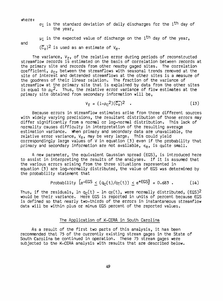
where:GI is the standard deviation of daily discharges for the i^h day of

the year,

Hi is the expected value of discharge on the i^n day of the year, and _

(Cv ) 2 is used as an estimate of Ve .

The variance, Vr , of the relative error during periods of reconstructed streamflow records is estimated on the basis of correlation between records at the primary site and records from other nearby gaged sites. The correlation coefficient, pc , between the streamflows with seasonal trends removed at the site of interest and detrended streamflows at the other sites is a measure of the goodness of their linear relation. The fraction of the variance of streamflow at the primary site that is explained by data from the other sites is equal to pc2 . Thus, the relative error variance of flow estimates at the primary site obtained from secondary information will be,

Vr = (l-Pc2 )(C7)2 . (13)

Because errors in streamflow estimates arise from three different sources with widely varying precisions, the resultant distribution of those errors may differ significantly from a normal or log-normal distribution. This lack of normality causes difficulty in interpretation of the resulting average estimation variance. When primary and secondary data are unavailable, the relative error variance, Ve , may be very large. This could yield correspondingly large values of V in equation [3) even if the probability that primary and secondary information are not available, ee , is quite small.

A new parameter, the equivalent Gaussian spread (EGS), is introduced here to assist in interpreting the results of the analyses. If it is assumed that the various errors arising from the three situations represented in equation (3) are log-normally distributed, the value of EGS was determined by the probability statement that

Probability [e-EGS £ (qc(t)/qT (t)) < e+EGS] = 0.683 . (14)

Thus, if the residuals, In qc (t) - In qy(t), were normally distributed, (EGS) 2 would be their variance. Here EGS is reported in units of percent because EGS is defined so that nearly two-thirds of the errors in instantaneous streamflow data will be within plus or minus EGS percent of the reported values.

The Application of K-CERA in South Carolina

As a result of the first two parts of this analysis, it has been recommended that 75 of the currently existing stream gages in the State of South Carolina be continued in operation. These 75 stream gages were subjected to the K-CERA analysis with results that are described below.

49

Definition of Missing Record Probabilities

As was described earlier, the statistical characteristics of missing stage or other correlative data for computation of streamflow records can be defined by a single parameter, the value of k in the truncated negative exponential probability distribution of times to failure of the equipment. In the representation of fr as given in equation (4), the average time to failure is 1/k. The value of lA will vary from site to site depending upon the type of equipment at the site and upon its exposure to natural elements and vandalism. The value of 1/k can be changed by advances in the technology of data collection and recording. To estimate 1/k in South Carolina, a 5-year period of actual data collection was used. Stream gages were visited on a consistent pattern during this 5-year period and a gage could be expected to be malfunctioning 6.2 and 5.3 percent of the time based on 6-week and monthly visitations, respectively. There was no reason to distinguish between gages on the basis of their exposure or equipment, so the 6.2 and 5.3 percent lost record with 6-week and monthly visitations were used to determine a value of lA of 365 days, which was used to determine ef, ee > anci e r f° r 71 °f the 75 stream gages as a function of the individual frequencies of visit.

Four stations (02148315, 02156500, 02160105, and 02160700), however, were visited 52 times per year for water-quality monitoring and were measured for discharge only eight times on those visits. In order to optimize over the number of discharge measurements made, two uncertainty curves were stored for each of the four stations. One curve was constant due to the uncertainty contributed by lost record when the stations were visited weekly. This constant value is given by

= PC(52)VC + Pn(52)Vn , (15)

where:

vlost(52) is the total variance of the error based on 52 visits per year,

Pc (52) is the probability of reconstructing streamflow data from nearby sites based on 52 visits per year,

Vc is the variance of the error during periods of reconstructed streamflow records,

Pn(52) is the probability of unavailable data for thereconstruction of streamflow records based on 52 visits per year,

and

Vn is the variance of the error during periods of unavailable data for reconstruction of streamflow records.

The second uncertainty curve for each of the four stations was obtained by using the process variance, the measurement variance, and the 1-day autocorrelation coefficient parameters from the rating residuals. The uncertainty from the lost record was not considered in this curve. The total uncertainty for each station was weighted from the two curves.

50

Definition of Cross-Correlation Coefficient and Coefficient of Variation

To compute the values of Ve and Vr of the needed uncertainty fuctions, daily streamflow records for each of the 75 stations for the last 30 years or the part of the last 30 years for which daily streamflow values are stored in WATSTORE (Hutchinson, 1975) were retrieved. For each of the stream gages that had three or more complete water years of data, the value of Cv was computed and various options, based on combinations of other stream gages, were explored to determine the maximum pc. For the 12 stations that had less than three water years of data, values of Cv and pc were estimated subjectively. In addition to other nearby stream gages, some of the stations have other means by which streamflow data can be reconstructed when the primary recorder malfunctions. Eight stations are equipped with telemetry systems that operate independently from the primary recorder and are routinely queried either once or twice per day. At another station, a local resident reads and records stage once or twice daily. Two sites have an auxiliary recorder to provide backup stage record.

Analyses were performed to determine cross correlation, pc, between daily discharges at sites with one or another of these types of auxiliary records by Fontaine and others (1983). For the case of daily or twice-daily readings of stage (observer or telemetry) a value of 0.96 or 0.99 was assigned to pc , respectively. For the case of supplemental recorders at stations a value of 0.99 was assigned to pc because very little record was lost.

The set of parameters for each station and the auxiliary records that gave the highest cross correlation coefficient are listed in table 10.

Kalman-Filter Definition of Variance

The determination of the variance Vf for each of the 75 stream gages required the execution of three distinct stepsi

1. long-term streamflow rating analysis and computation of residuals of measured discharges from the long-term rating;

2. time-series analysis of the residuals to determine the input parameters of the Kalman-filter streamflow records; and

3. computation of the error variance, Vf, as a function of the time-series parameters, the discharge-measurement-error variance, and the frequency of discharge measurement.

In the South Carolina program analysis, a single rating function was used to define the entire year for long-term ratings. Existing rating curves, in most cases, defined the long-term rating function required in the analysis. In the cases where this was not true, the shifts in the curves have been extensions at the high end of the curves or slight adjustments in the extreme low ends of the curves. In these cases, a mean curve was determined graphically.

51

Table 10. Statistics of record reconstruction

Station number

0211050002129590021309000213091002131000021311500213130902131472*02132000021350000213530002135500021360000214600002147000021480000214831502153780*02154500021555000215605002156450*0215650002157000021601050216070002160775*02161000*02161700*021620100216209302162350*02162525*021635000216500002166970*02167000021690000216950002169570021696300217050002171500021715600217165002171680

Cv

1.19391.39700.64880.49710.72401.20671.0065

- 0.730.85030.91140.83641.19771.39700.76490.69300.78500.46470.730.86650.93470.97760.730.90981.05130.73320.75520.740.980.730.74600.63040.750.750.79130.97560.740.77490.77490.84100.97560.97560.63040.86650.97561.75061.8598

PC

0.77230.94760.88520.89670.73830.63870.68830.860.950.77230.75710.82670.82670.87820.87820.990.990.860.93000.93000.83930.860.990.79830.990.990.610.990.860.60900.91380.450.450.72060.74310.610.990.990.990.64990.60810.86520.44810.49560.72630.5070

Source of reconstructed records

135000 136000136000130910131309 135300 130900132000135500130900

Observer; read daily110500135500136000135500147000146000TelemetryTelemetry

155500154500161500

Telemetry154500TelemetryTelemetry

Telemetry

132000173000

161500169570

Supplemental recorder at siteSupplemental recorder at siteTelemetry169630169570169500171560171500171500171650

52

Table 10. Statistics of record reconstruction Continued

Station number

02172640*021730000217350002174000021750000217550002176500021768750218520002196250*021970000219730002197310021973150219732002197326021973300219733202197334021973360219733802197339*02197340021973420219734402197348021973590219740002198500

cv

0.630.63040.54720.62390.88110.77741.52640.77740.74600.420.45450.23830.30050.30500.37630.16610.37710.47070.68450.61770.34830.350.54410.59910.51290.45800.47670.53270.7770

PC

0.920.91600.93460.93460.92440.84480.74320.74320.44920.660.990.60960.85260.85260.45280.74660.32120.39020.86700.89980.42820.430.89980.86700.18260.11720.46370.51490.7432

Source of reconstructed records

173500174000173500174000174000

174000

Telemetry197400197315197310197315197330197310197340197342197340197340

197346197334197338197342197400173000197000

*Less than 3 years of data are available, subjective.

Estimates of Cv and pc are

53

Results of the rating analysis of many stream-gaging stations often yield ratings about which there were large amounts of variance, but some of the ratings had tight fits about the available discharge. The rating curves were developed using discharge in cubic feet per second and the residuals were converted to logarithmic units (base 10) before the autocovariance analysis.

The time series of residuals was used to compute sample estimates of q and $, two of the three parameters required to compute Vf, by determining a best fit autocovariance function to the time series of residuals. Measurement variance, the third parameter, was determined for individual stations. If a measurement had a rating of excellent it was assigned a value of 2 percent error. Measurements with ratings of good and fair were assumed to have errors of 5 percent and 8 percent, respectively. Poor measurements were assigned a value greater than 8 percent. These ratings were weighted and an average value was given to each station.

As discussed earlier, q and $ can be expressed as the process variance of the shifts from the rating curve and the 1-day autocorrelation coefficient of these shifts. Table 9 presents a summary of the autocovariance analysis expressed in terms of process variance and 1-day autocorrelation. Typical fits of the autocovariance functions for selected stations in South Carolina are given in figures 6 and 7.

The autocovariance parameters, summarized in table 11, and data from the definition of missing record probabilities, summarized in table 10, are used jointly to define uncertainty functions for each gaging station. The uncertainty functions give the relation of total error variance to the number of visits and discharge measurements. Uncertainty functions for the stations for which graphical fits of the autocovariance functions were previously given are presented as typical examples in figure 8. These functions are based on the assumption that a measurement was made during each visit to the station.

54

:OVARIANCE

p o o c

b b b c2 ° -* o 01 o o

^ -0.005

-0.010 (

I I I I '! I I I

o

o

° 0 0°0 °

. ..II."" ""0 0

00

I I I I 1 t I I I

3 5 10 15 20 25 30 35 40 45 5(

LAG, IN DAYS

F

0.150

0.100UJU^ 0.050

2< 0.000

O^ -0.050

-0.100

0

igure 6. Autocovariance function for station 02160700

i i i i i i i i i

~ o

o0 <

- o

^ 000^.0 ooo^ 1^0 0 o 0 0

0 0 0 ^ 0o o X

0_ o _

0

1 1 1 1 1 1 1 1 15 10 15 20 25 30 35 40 45 5C

LAG, IN DAYS

Figure 7.--Autocovariance function for station 02171680

55

18

0

H

16

0z UJ U

140

DC

UJ *

120

tf

100

O eg Ctf

80

UJ §

60

Q 24

0

20

EX

PL

AN

AT

ION

ST

AT

ION

02171680

02160700

0 5

10

15

20

25

30

35

40

45

50

NU

MB

ER

OF

VIS

ITS

AN

D M

EA

SUR

EM

EN

TS

PE

R Y

EA

R

figu

re 8

. Typical

unce

rtai

nty

function for

instantaneous

disc

harg

e

Table 11. Summary of the autocovariance analysis

Station number

021105000212959002130900021309100213100002131150021313090213147202132000021350000213530002135500021360000214600002147000021480000214831502153780021545000215550002156050021564500215650002157000021601050216070002160775021610000216170002162010021620930216235002162525021635000216500002166970021670000216900002169500021695700216963002170500021715000217156002171650

Rho*

0.9750.9740.9190.9860.8850.9820.9800.9850.9570.9750.9800.9850.9710.9710.9550.9820.9780.99-70.9920.9830.9570.9610.9920.9870.9780.9860.9290.9790.9860.9920.8560.9880.9670.9770.9860.9770.9490.9550.9660.9800.9800.8940.9930.9800.994

Measurement variance

(log base 10 ) 2

7.5x10~56.4x10"48.1x10~44.7x10"41.2x10~37.8x10~46.9x10~46.0x10~44.7x10~46.6x10~46.8x10~41.1x10~37.9x10~48.1x10"48.7x10~47.3x10~45.7x10~48.6x10"44.7x10"44.7x10~46.9x10~47.1x10"44.7x10~44.7x10~45.6x10~45.7x10~48.1x10~48.5x10~47.5x10"47.9x10~48.7x10~48.6x10~46.3x10"44.7x10~46.7x10~48.7x10~47.7x10~49.9x10~46.6x10~45.9x10~44.7x10~44.9x10~45.1x10"46.4x10"45.6x10~4

Process variance

(log base 10 ) 2

1.7x10"36.0x10~32.1x10"34.7x10~41.5x10~32.9x10~29.6x10~31.8x10~34.2x10~41.7x10~31.6x10~31.1x10~23.5x10~ 31.3x10~35.9x10~31.8x10~26.6x10~46.7x10~36.7x10"49.7x10~48.9x10~ 31.8x10~27.6x10~47.8x10~48.3x10~43.4x10~46.1x10~39.4x10~45.1x10~25.1x10~23.6x10~33.7x10~41.3x10~25.4x10~31.1x10~21.7x10~24.4x10~33.1x10~38.7x10~43.8x10~36.6x10~41.2x10~34.8x10~31.1x10~33.1x10~3

57

Table 11. Summary of the autocovariance analysis Continued

Station number

021716800217264002173000021735000217400002175000021755000217650002176875021852000219625002197000021973000219731002197315021973200219732602197330021973320219733402197336021973380219733902197340021973420219734402197348021973590219740002198500

Rho*

0.9730.9800.9610.9810.9850.6010.9830.9820.9790.9730.9630.9230.9850.9920.9750.9860.9870.9770.9560.5620.9840.9830.9960.9920.9670.9830.9930.9260.9780.969

Measurement variance

(log base 10 ) 2

1.3x10"34.9x10"46.1x10"44.9x10~49.2x10"44.7x10"46.6x10~41.3x10"31.1x10"34.7x10"46.1x10"45.9x10"44.8x10~44.7x10"45.8x10-44.7x10"45.8x10"44.7x10"46.8x10~44.7x10~47.6x10~44.7x10"46.8x10~41.2x10~35.1x10~45.9x10~44.9x10~44.7x10~49.2x10"43.0x10~4

Process variance

(log base 10 ) 2

1.9x10~22.5x10~31.8x10~31.0x10~51.0x10~56.1x10~41.1x10~32.7x10~21.4x10~25.3x10~41.4x10~29.0x10~41.5x10~32.4x10~49.2x10~44.0x10~ 53.9x10~ 34.5x10~31.0x10~26.3x10~48.4x10~ 38.4x10~35.4x10~25.5x10~22.0x10~58.5x10~43.3x10~32.tx10~34.6x10~ 32.4x10~4

*One-day autocorrelation coefficient.

58

Determination of Routes and Costs

In South Carolina, feasible routes to service the 75 stream gages were determined after consultation with personnel in the Hydrologic Data Section of the South Carolina office and after review of the uncertainty funtions. In summary, 77 routes were selected to service all the stream gages in South Carolina. These routes included all possible combinations that describe the current operating practice, alternatives that were under consideration as future possibilities, routes that visited certain key individual stations, and combinations that grouped gages where the levels of uncertainty indicated more frequent visits might be useful. These routes and the stations visited are summarized in table 12. Negative numbers in table 12 were assigned to stations other than stream-gaging stations, that is, water quality, stage only, crest-stage, and ground water.

The cost associated with the established routes was determined from previous expense records. Vehicle rental, mileage, maintenance, hydrographer salary, and per diem were included in the travel costs. Fixed costs to operate a gage typically include equipment rental, batteries, electricity, data processing and storage, computer charges, maintenance and miscellaneous supplies, and analysis and supervisory charges. For South Carolina, average values were applied to each station in the program for all the above categories based on past experience.

Visit costs are those associated with paying the hydrographer for the time actually spent at a station servicing the equipment and making a discharge measurement. Average visit times were calculated for each station based on an analysis of available discharge measurement data. This time was then multiplied by the average hourly salary of hydrographers in the South Carolina office to determine total visit costs.

Route costs include the vehicle cost associated with traveling the number of miles in the route, the cost of the hydrographer's time while in transit, and any per diem associated with the trip.

59

Table 12. Summary of the routes that may be used to visit stations in South Carolina [Negative numbers represent stations other than surface-water stations]

Route Stations serviced on the route

number________________________________________________________

1 -1* 02110500 -2 -3 02135000 -4 -5-6 -7 -8 02129590 -9 02131150 02131000

-10 -11 -12 -13 -14 02132000 -1502136000 -16 -17 -18 -19 02171560 02171680

2 02110500 02135000 02131000 02131150 02129590 02132000 0213600002171560 02171680

3 -1 02110500 -2 -3 02135000 -4 -5-6 -7 -8 -9 -10 -11 -12

-13 -14 02132000

4 02110500 02135000 02129590 02131150 02131000 02132000

5 -15 02136000 -16 -17 -18 02171500 -19 02171560 02170500 02171650 02171680

6 02136000 02171500 02171560 02170500 02171650 02171680

7 -1 02110500 -2 -3 02135000

8 02135000 02131150

9 02129590 02131150

10 02129590 02131150 02135000

11 02131150 02131000 02135000

12 02135000 02131000 02132000

13 -20 02148000 02131472 -21 02131309 02147000 02146000-22 02153780 -23 02156450 -24 02161700 02160775

14 02148000 02131472 02131309 02147000 02146000 02153780 0215645002161700 02160775

15 02162093 02162010 -24 02131309 -21 02131472 02148000-20 -25

16 02162093 02162010 02148000 02131472 02131309

17 02161000 02160775 02160700 02160105 02156500 02161700 02162010

60

Table 12. Summary of the routes that may be used to visit stations in South Carolina Continued [Negative numbers represent stations other 'thansurface-water stations]


number__________________________________________________________

18 02162093 02162010 02161700 02156500 02156450 02153780

19 02131309 02131472

20 02146000 02147000

21 02153780 02156450

22 02175000 02176500

23 -25 -26 02156500 02160105 02160700 -27 02161000

24 02162010 -28 -29 -30 -31 02157000 -3202156050 02154500 02155500 -33 -34

25 02162010 02157000 02156050 02154500 02155500

26 02162010 02161000 -28 -29 -30 -31 0215700002156050 02154500 02155500 -33 -34 -23 0215645002156500 02160105 02160700 02160775

27 02162010 02161000 02157000 02156050 02154500 02155500 0215645002156500 02160105 02160700 02160775

28 02162010 02161000 -29 -30 -31 02167000 -3202156050 02154500 02155500 -33 -34 -23 0216010502160700 02160775

29 02162010 02161000 02167000 02156050 02154500 02155500 0216010502160700 02160775

30 02162010 02161000

31 02156050 02157000

32 02167000 02166970 02163500 02105000 -35 -36 -37-38 -39 -40 -41 -42 -43 -44-45 02162525 -46 02162350 02185200 -47 -48-49 -50 02196250 02197000

33 02167000 02166970 02163500 02165000 02162525 02162350 0218520002196250 02197000

34 02167000 02166970 02163500 02165000 -35 -48 -49-50 02196250 02197000

61

Table 12. Summary of the routes that may be used to visit stations in South Carolina Continued [Negative numbers represent stations other than surface-water stations]


number__________________________________________________________

35 -39 -40 -38 -41 -42 -43 -44-45 02162525 -46 02162350 02185200 -47 -36

36 02165000 02163500 02166970 02167000

37 02165000 02167000

38 02165000 02163500

39 02162350 02162525

40 -51 02172640 -52 -53 02198500 -56 -57-58 -59 -60 -61 -62 -63 -64

02175500 -55 02173000 -54

41 02169630 02174000 -65 -66 -67 -68 -69-70

42 02169630 02173500

43 02169630 02173500 02174000

44 02172640 02173000

45 02173000 02175500

46 02198500 02176875

47 02173000 02198500 02176875

48 02148000 02135300

49 -71 -72 -73 -74 -75 -76 -77-78 -79 02130900 02130910 -80 -81 02135500-82 02169570 02162093 02169000 02169500

50 02130900 02130910 02135500 02169570 02162093 02169000 02169500

51 02135300 02175000 -83 -84 02176500 -85 02176875-86

52 02169570 02135300 02131000 02132000 02135500

62

Table 12. Summary of the routes that may be used to visit stations in South Carolina--Continued [Negative numbers represent stations other than surface-water stations]


number__________________________________________________________

53 02197300 02197310 02197315 02197320 02197326 02197330 0219733202197334 02197336 02197338 02197339 02197340 02197342 0219734402197348 02197359 02197400 -87 -88 -89 -90

-91 -92 -94 -95 -96 -97

54 02197300 02197310 02197315 02197320 02197326 02197330 0219733202197334 02197336 02197338 02197339 02197340 02197342 0219734402197348 02197359 02197400

55 02148315 -93 02170500 02171500 02171650

56 02110500

57 02129590

58 02131150

59 02135500

60 02156450

61 02160775

62 02173500

63 02162010

64 02166970

65 02169570

66 02171500

67 02171560

68 02171650

69 02171680

70 02176500

71 02176875

72 02196250

63

Table 12. Summary of the routes that may be used to visit stations in South Carolina Continued [Negative numbers represent stations other than surface-water stations]


number__________________________________________________________

73 02148315

74 02156500

75 02160105

76 02160700

77 02161000

64

K-CERA Results

The "Traveling Hydrographer Program" utilizes the uncertainty functions, appropriate cost data and route definitions to compute the most cost-effective way to operate the stream-gaging program. In this application, the first step was to simulate the current practice and determine the total uncertainty associated with it. To accomplish this, the number of visits being made to each stream gage and the specific routes being used to make these visits were fixed. In South Carolina, current practice indicates that discharge measurements are made on approximately 50 percent of the visits for 17 stations and 95 percent for 58 stations. These values were determined from past records. The resulting average error of estimation for the current practice in South Carolina is plotted as a point in figure 9 and is 16.9 percent.

The solid line on figure 9 represents the minimum level of average uncertainty that can be obtained for a given budget with the existing instrumentation and technology. The line was defined by several runs of the "Traveling Hydrographer Program" with different budgets. Constraints on the operations other than budget were defined as described below.

To determine the minimum number of times each station must be visited, consideration was given only to the physical limitations of the method used to record data. The effect of visitation frequency on the accuracy of the data and the amount of lost record is taken into account in the uncertainty analysis. Minimum visit requirements should also reflect the need to visit stations for special reasons such as water-quality sampling. Several stations in South Carolina have multiple functions, that is, stage only and quality of water, or discharge and quality of water. In South Carolina, minimum visit requirements of 4 and 12 visits per year were selected and applied to the appropriate stations.

The results in figure 9 and table 13 summarize the K-CERA analysis and are predicated on a discharge measurement being made each time that a station is visited. This is a change from the current policy under which a measurement is made on an overall average of 85 percent of the visits. It should be emphasized that figure 9 and table 11 are based on various assumptions (stated previously) concerning both the time series of shifts to the stage-discharge relation and the methods of reconstruction.

It can be seen that the current policy results in an average standard error of estimate of streamflow of 16.9 percent. This policy requires a budget of $417,200 to operate the 75-station stream-gaging program and stage-only and crest-stage stations. The range in standard errors is from a low of 2.3 percent for station 02160700, to a high of 44.8 percent for station 02171680. It is possible to obtain this same average standard error with a reduced budget of about $395,000 with a change in policy in the field activities of the stream-gaging program. This policy and budget change would result in a decrease in standard error from 2.3 to 1.2 percent at station 02160700, while the standard error at station 02171680 would decrease from 44.8 to 31.5 percent. However, these two stations would still have the extreme values of standard error.

It also would be possible to reduce the average standard error by a policy change while maintaining the same budget of $417,200. In this case, the average would decrease from 16.9 to 15.5 percent. Extremes of standard errors for individual sites would be 2.7 and 31.5 percent for stations 02160700 and 02171680, respectively.

65

H

2 UJ

35

U

CC

UJ

ft-

30

§ 25

05 06 UJ

20

Q

CC a z UJ O <

tf

UJ > <

15 10

0 C

urr

ent

pra

ctic

e

i1

wit

h m

issi

ng

reco

rd

wit

hou

t m

issi

ng

reco

rd

I4

00

5

00

6

00

700

80

0

BUDGET, IN THOUSANDS OF 1983 DOLLARS

90

0

Fig

ure

9.-

-Ave

rage

sta

nd

ard

err

or

per

stre

am-g

age

Table 13. Selected results of K-CERA analysis

Identification

Average perstation*

02110500

02129590

02130900

02130910

02131000

02131150

02131309

02131472

02132000

02135000

Standard error of instantaneous discharge, in percent [Equivalent Gaussian spread]

(Number of visits per year to site)Current

operation

16.9[8.5]

20.0[6.6](8)

19.7[17.6](8)

11.7[9.8](8)

6.3[2.8](8)

14.8[9.3](8)

31.4[23.4](8)

22.3[14.3](8)

11.5[5.7](8)

13.3[4.7](8)

15.6[6.7](8)

383.5

18.6[9.5]

22.8[7.5](6)

22.5[19.1](4)

13.9[11.0](4)

8.6[3.9](4)

18.7[10.1](4)

31.4[23.4](8)

23.6[15.2](7)

12.4[6.0](7)

14.1[4.8](7)

16.6[7.1](7)

Budget, in| 395

16.9[8.9]

18.9[6.2](9)

22.5[19.1](4)

13.9[11.0](4)

8.6[3.9](4)

17.3[9.8](5)

26.0[19.0](12)

21.1[13.5](9)

10.8[5.3](9)

16.3[5.1](5)

14.8[6.4](9)

thousands of 1983 dollars| 417.2

15.5[8.2]

18.9[6.2](9)

19.2[17.3](9)

12.6[10.3](6)

7.2[3.3](6)

13.4[9.0]

(11)

25.0[18.2]

(13)

19.3[12.2](11)

9.8[4.8]

(11)

11.6[4.4]

(11)

12.5[5.4]

(13)

600

9.8[5.3]

9.6[3.1]

(36)

15.6[14.6](24)

9.3[8.1]

(17)

4.4[2.0]

(17)

11.1[8.4]

(21)

13.6[9.6]

(46)

11.1[6.8]

(35)

5.4[2.8]

(35)

8.7[3.8]

(21)

7.5[3.3]

(38)

850

7.6[4.1]

7.0[2.3]

(69)

11.1[10.4](65)

7.0[6.1]

(37)

3.0[1.3]

(37)

8.9[7.4]

(47)

10.2[7.2]

(82)

8.3[5.1]

(64)

4.0[2.1]

(64)

6.2[3.0](6.1)

5.5[2.5]

(70)

67

Table 13. Selected results of K-CERA analysis Continued

Identification

02135300

02135500

02136000

02146000

02147000

02148000

02148315

02153780

02154500

02155500

02156050

Standard error of instantaneous discharge, in [Equivalent Gaussian spread]


operation

15.3[7.8](8)

20.6[13.3](8)

21.5[10.0](8)

10.7[6.2](8)

15.6[14.4](8)

16.3[15.3](8)

3.7[3.6](8)

11.3[5.1](8)

11.2[8.7](8)

9.4[4.4](8)

17.4[12.4](8)

Budget/ in383.5

17.1[8.1](6)

25.4[16.7](5)

21.5[10.0](8)

13.0[7.3](5)

17.7[16.2](5)

18.7[17.3](6)

4.6[4.4](4)

13.3[6.0](6)

15.2[12.4](4)

12.8[6.0](4)

23.2[17.2](4)

395

16.1[7.9](7)

20.6[13.3](8)

22.8[10.5](7)

13.0[7.3](5)

17.7[16.2](5)

16.3[15.3](8)

4.5[4.5](4)

11.3[5.1](8)

13.8[11.1](5)

11.6[5.4](5)

19.7[14.3](6)

thousands ofI 417.2

14.6[7.6](9)

19.5[12.5](9)

16.1[7.6]

(15)

9.7[5.6]

(10)

14.6[13.4](10)

13.9[13.3](11)

4.6[4.5](4)

10.0[4.5]

(10)

11.9[9.4](7)

10.0[4.6](7)

18.4[13.2](7)

percent

1983 dollarsI 600

9.2[6.0]

(30)

11.0[6.9]

(30)

10.3[4.9]

(38)

7.4[4.4]

(18)

11.7[10.7](18)

8.2[8.1]

(32)

3.8[3.8](7)

8.1[3.7]

(15)

7.5[5.6]

(19)

6.3[2.9]

(19)

10.8[7.5]

(22)

| 850

7.3[5.1]

(53)

8.0[5.0]

(58)

7.4[3.5]

(75)

5.3[3.2]

(36)

8.7[7.9]

(36)

6.4[6.3]

(54)

2.7[2.7]

(17)

6.2[2.9]

(25)

5.7[4.2]

(34)

4.7[2.2]

(34)

8.0[5.5]

(41)

68


Identification

02156450

02156500

02157000

02160105

02160700

02160775

02161000

02161700

02162010

02162093

02162350



operation

24.9[24.1](8)

3.6[3.3](8)

16.1[3.5](8)

4.2[4.0](8)

2.3[1.2](8)

21.2[16.5](8)

8.8[4.6](8)

27.3[26.8](8)

24.9[21.9](8)

14.1[13.5](8)

17.1[3.8](8)

Budget, in thousands of 1983 dollars383.5

27.1[26.2](6)

3.6[3.6](6)

22.2[5.0](4)

4.8[4.7](5)

2.7[0.45](5)

23.2[17.6](6)

12.5[5.5](5)

29.1[28.5](7)

24.9[21.9](8)

15.0[14.2](5)

21.4[4.5](5)

395

26.0[25.1](7)

3.6[3.6](6)

18.4[4.1](6)

4.8[4.7](5)

1.2[1.2](4)

23.2[17.6](6)

12.5[5.5](5)

27.3[26.7](8)

20.5[17.6](12)

14.6[13.9](6)

19.6[4.2](6)

417.2

22.3[21.6](11)

4.1[3.6](5)

17.1[3.8](7)

4.8[4.7](5)

2.7[1.2](5)

19.1[15.2](11)

10.9[5.2](6)

24.6[24.0](10)

20.5[17.6](12)

14.4[13.7](7)

15.4[3.6]

(10)

600

13.0[12.5](37)

3.6[3.6](6)

9.9[2.2]

(22)

3.8[3.8](9)

1.2[1.2](4)

11.8[9.8]

(37)

5.6[3.5]

(15)

24.6[24.0](10)

11.3[9.3]

(41)

12.2[11.9](19)

9.7[2.5]

(26)

850

10.1[9.6]

(63)

2.6[2.6]

(15)

7.3[1.6]

(41)

2.7[2.7]

(21)

1.2[1.2](4)

8.6[7.1]

(74)

4.0[2.8]

(25)

24.6[24.0](10)

8.6[7.1]

(73)

9.8[9.5]

(42)

6.9[1.9]

(51)

69


Identification

02162525

02163500

02165000

02166970

02167000

02169000

02169500

02169570

02169630

02170500

02171500

Standard error of instantaneous discharge, in [Equivalent Gaussian spread]


operation

24.7[19.9](8)

17.0[11.2](8)

20.7[14.2](8)

23.6[20.0](8)

12.3[12.3](8)

10.0[10.0](8)

8.1[5.1](8)

20.2[9.0](8)

11.6[3.9](8)

10.6[7.9](8)

20.1[6.4](8)

Budget, in thousands of383.5

29.3[23.4](5)

20.7[13.8](5)

25.5[17.9](5)

28.5[24.3](5)

13.3[13.2](5)

11.7[11.7](4)

13.2[6.3](4)

21.4[9.6](7)

14.6[4.8](5)

10.0[7.6]

(10)

18.1[5.7]

(10)

| 395

27.5[22.1](6)

17.0[11.2](8)

20.7[14.2](8)

25.0[21.2](7)

13.0[13.0](6)

11.7[11.7](4)

13.2[6.3](4)

17.4[7.8]

(11)

14.6[4.8](5)

10.0[7.6]

(10)

18.1[5.7]

(10)

417.2

22.6[18.2](10)

15.4[10.2](10)

18.7[12.6](10)

21.5[18.1](10)

11.6[11.3](10)

10.7[10.7](6)

9.9[5.6](6)

18.2[8.1]

(10)

14.6[4.8](5)

10.0[7.6]

(10)

18.1[5.7]

(10)

percent

1983 dollars] 600

14.7[11.7](26)

9.1[5.9]

(31)

10.9[7.1]

(31)

12.2[10.0](33)

8.6[8.6]

(24)

7.9[7.9]

(17)

5.1[3.9]

(17)

8.4[3.8]

(49)

7.6[2.6]

(19)

7.4[6.0]

(25)

11.0[3.4]

(28)

| 850

10.6[8.3]

(51)

7.0[4.5]

(53)

7.9[5.1]

(60)

9.4[7.7]

(57)

6.6[6.6]

(45)

5.8[5.7]

(37)

3.3[2.7]

(37)

6.4[2.9]

(86)

5.6[1.9]

(35)

6.1[5.1]

(41)

8.2[2.5]

(51)

70


Identification

02171560

02171650

02171680

02172640

02173000

02173500

02174000

02175000

02175500

02176500

02176875



operation

21.6[4.9](8)

30.3[4.9](8)

44.8[22.6](8)

10.0[7.3](8)

9.5[7.8](8)

5.9[0.13]

(12)

5.5[0.44](8)

10.0[6.0](8)

11.2[4.7](8)

32.8[23.0](8)

21.1[17.6](8)

Budget, in thousands of383.5 |

21.6[4.9](8)

27.2[4.3]

(10)

40.4[20.4](10)

14.3[9.8](4)

11.9[9.6](4)

8.1[0.23](4)

7.7[0.62](4)

12.7[6.5](4)

15.3[6.5](4)

37.2[26.4](6)

27.9[23.4](4)

395 | 417.2

21.6 15.9[4.9] [3.7](8) (15)

26.0 26.0[4.1] [4.1]

(11) (11)

31.5 31.5[15.8] [15.8](17) (17)

14.3 11.6[9.8] [8.3](4) (6)

11.1 10.5[9.1] [8.8](5) (6)

8.1 7.3[0.23] [0.20](4) (5)

7.7 6.9[0.62] [0.55](4) (5)

12.7 10.4[6.5] [6.1](4) (7)

15.3 12.8[6.5] [6.2](4) (6)

29.6 31.1[20.5] [21.7](10) (9)

22.3 21.1[18.7] [17.6](7) (8)

1983 dollars| 600 |

10.1[2.4]

(38)

13.6[2.1]

(41)

16.8[8.4]

(62)

7.3[5.5]

(15)

6.0[5.0]

(25)

4.4[0.11]

(15)

5.5[0.44](8)

10.0[6.0](8)

9.3[3.9]

(12)

15.0[10.0](41)

12.0[9.8]

(27)

850

7.2[1.7]

(75)

10.2[1.6]

(74)

12.7[6.4]

(110)

5.4[4.1]

(28)

4.4[3.6]

(50)

3.1[0.08]

(31)

4.1[0.33]

(15)

8.0[5.7]

(16)

6.8[2.9]

(23)

12.0[8.0]

(66)

8.7[7.1]

(52)

71


Identification

02185200

02196250

02197000

02197300

02197310

02197315

02197320

02197326

02197330

02197332

02197334



operation

17.0[3.9](8)

21.0[20.6](8)

7.1[6.3](8)

6.6[5.4]

(12)

4.2[1.8]

(12)

4.8[4.8]

(12)

7.8[0.91]

(12)

8.1[8.0]

(12)

13.1[11.0](12)

21.0[19.7](12)

9.6[6.1]

(12)

Budget, in thousands of383.5

21.1[4.7](5)

25.0[24.5](4)

9.0[6.7](4)

6.6[5.4]

(12)

4.2[1.8]

(12)

4.8[4.7]

(12)

7.8[0.91

(12)

8.1[8.0]

(12)

13.1[11.0](12)

21.0[19.7](12)

9.6[6.1]

(12)

| 395

21.1[4.7](5)

23.8[23.4](5)

8.2[6.6](5)

6.6[5.4]

(12)

4.2[1.8]

(12)

4.8[4.7]

(12)

7.8] [0.91]

(12)

8.1[8.0]

(12)

13.1[11.0](12)

21.0[19.7](12)

9.6[6.1]

(12)

417.2

15.2[3.5]

(10)

19.5[19.0](10)

6.7[6.1]

(10)

6.6[5.4]

(12)

4.2[1.8]

(12)

4.8[4.7]

(12)

7.8[0.91]

(12)

8.1[8.0]

(12)

13.1[11.0](12)

21.0[19.7](12)

9.6[6.1]

(12)

1983 dollars600

11.2[2.7]

(19)

12.0[11.6](31)

5.7[5.5]

(18)

4.2[3.4]

(34)

2.5[1.1]

(34)

3.3[3.3]

(34)

4.7[0.56]

(34)

5.1[5.0]

(34)

8.4[6.9]

(34)

14.7[13.8](34)

7.2[5.7]

(34)

850

8.7[2.1]

(32)

8.7[8.3]

(61)

4.7[4.6]

(33)

3.2[2.5]

(62)

1.8[0.79)

(62)

2.6[2.6]

(62)

3.5[0.42]

(62)

3.9[3.9]

(62)

6.3[5.2]

(62)

11.3[10.5](62)

6.4[5.4]

(62)

72


Identification

02197336

02197338

02197339

02197340

02197342

02197344

02197348

02197359

02197400

02198500

Standard error of instantaneous discharge/ in percent [Equivalent Gaussian spread]


operation

13.6[12.9](12)

14.4[13.2](12)

17.3[16.7](12)

23.2[23.2](12)

6.9[0.85]

(12)

12.3[4.4]

(12)

11.7[5.8]

(12)

13.3[9.8]

(12)

14.7[11.0](12)

13.8[2.7](8)

Budget, in thousands of 1983 dollars383.5 |

13.6[12.9](12)

14.4[13.2](12)

17.3[16.7](12)

23.2[23.2](12)

6.9[0.85]

(12)

12.3[4.4]

(12)

11.7[5.8]

(12)

13.3[9.8]

(12)

14.7[11.0](12)

19.8[3.6](4)

395 | 417.2

13.6 13.6[12.9] [12.9](12) (12)

14.4 14.4[13.2] [13.2](12) (12)

17.3 17.3[16.7] [16.7](12) (12)

23.2 23.2[23.2] [23.2](12) (12)

6.9 6.9[0.85] [0.85]

(12) (12)

12.3 12.3[4.4] [4.4]

(12) (12)

11.7 11.7

[5.8] [5.8](12) (12)

13.3 13.3

[9.8] [9.8](12) (12)

14.7 14.7[11.0] [11.0](12) (12)

14.8 14.8[2.9] [2.9](7) (7)

600 |

8.6[8.0]

(34)

9.0[8.1]

(34)

10.6[9.9]

(34)

14.0[13.9](34)

4.2[0.57]

(34)

7.5[2.8]

(34)

7.1[3.4]

(34)

9.3[7.5]

(34)

9.3[7.0]

(34)

7.6[1.6]

(26)

850

6.5[6.0]

(62)

6.8(6.1]

(62)

8.0[7.4]

(62)

10.5[10.4](62)

3.1[0.44]

(62)

5.6[2.1]

(62)

5.3[2.6]

(62)

7.3[6.1]

(62)

7.0[5.2]

(62)

5.4[1.2]

(50)

*Square root of seasonally averaged station variance,

73

A minimum budget of $383,500 is required to operate the 75-discharge station program, including stage-only and crest-stage stations. A budget less than this does not permit proper service and maintenance of the gages and recorders. Stations would have to be eliminated from the program if the budget fell below this minimum. At the minimum budget, the average standard error is 18.6 percent. The minimum standard error of 2.7 percent would occur at station 02160700, while the maximum of 40.4 percent would occur at station 02171680.

The maximum budget analyzed was $850,000, which resulted in an average standard error of estimate of 7.6 percent. Thus, more than doubling the budget in conjunction with policy change would reduce the average standard error in excess of 50 percent from the current policy and current budget. For the $850,000 budget, the extremes of standard error are 24.6 for station 02161700 and 1.8 percent for station 02197310. Thus, it is apparent that significant improvements in accuracy of streamflow records can be obtained if larger budgets become available.

The analysis also was performed under the assumption that no correlative data at a stream gage were lost because of less than perfect instrumentation. The average standard errors of estimation of streamflow that could be obtained if perfectly reliable systems were available to measure and record the correlative data are 9.5 percent for the minimal operational budget of $383,500. Here, the impacts of less than perfect equipment are greatest.

At the other budgetary extreme of $850,000, under which stations are visited more frequently and the reliability of equipment should be less sensitive, average standard errors are 4.1 percent for ideal equipment. Thus, improved equipment can have a positive impact on streamflow uncertainties throughout the range of operational budgets that possibly could be anticipated for the stream-gaging program in South Carolina.

Conclusions from the K-CERA Analysis

As a result of the K-CERA analysis, the following conclusions are offered:

1. The policy for the definition of field activities in the stream-gaging program should be altered to maintain the current average standard error of estimate of streamflow records of 16.9 percent with a budget of approximately $395,000. This shift would result in some increases and some decreases in accuracy of records at individual sites.

2. The amount of funding for stations with accuracies that are not acceptable for the data uses should be renegotiated with the data users.

3. The K-CERA analysis should be re-run with new stations included whenever sufficient information about the characteristics of new stations has been obtained.

4. Schemes for reducing the probabilities of missing record should be explored and evaluated as to their cost effectiveness in providing streamflow information. Several of these schemes are increased use of local gage observers, satellite relay of data, and backup recorder systems.

74

SUMMARY

Currently, 76 continuous-record stream gages are being operated in South Carolina at a cost of $422,200. Fifteen separate sources of funding contribute to this program and up to five separate uses were identified for data from a single gage.

In an analysis of the uses that are made of the data, station 02161500 was identified as having alternate methods of computing the streamflow record. Operation of this station should be discontinued. The remaining 75 stations should be maintained in the program for the foreseeable future.

The current policy for operation of the 75-discharge station program and the crest-stage and stage-only stations would require a budget of $417,200 per year. It was shown that the current overall level of accuracy of the records at these 75 sites could be maintained with approximately a $395,000 budget, including the stage-only and crest-stage gages, if the allocation of stream- gaging effort among gages was altered.

A major component of the error in streamflow records is caused by loss of primary record (stage or other correlative data) at the stream gages because of malfunctions of sensing and recording equipment. The upgrading of equipment and the development of strategies to minimize lost record appear to be key actions required to improve the reliability and accuracy of the streamflow data generated in the State.

Studies of the cost effectiveness of the stream-gaging program should be continued and should include investigation of the optimum ratio of discharge measurements to total site visits for each station, as well as investigation of cost-effective ways of reducing the probabilities of lost correlative data. Future studies also will be required because of changes in demands for streamflow information with subsequent addition and deletion of stream gages. Such changes will affect the operation of other stations in the program because of the dependence between stations of the information that is generated (data redundancy) and because of the dependence of the costs of collecting the data from which the information is derived.

75

REFERENCES CITED

Armbruster, J. T., 1970, A proposed streamflow data program for South Carolina? U.S. Geological Survey Open-File Report, 30 p.

Benson, M. A., and Carter, R. W., 1973, A national study of the streamflowdata-collection programs U.S. Geological Survey Water-Supply Paper 2028, 44 p.

Carter, R. W., and Benson, M. A., 1970, Concepts for the design of streamflow data programs! U.S. Geological Survey Open-File Report, 33 p.

Cooke, C. W., 1936, Geology of the Coastal Plain of South Carolina? U.S. Geological Survey Bulletin 867, 196 p.

Draper N. R., and Smith, H., 1966, Applied regression analysis! New York, John Wiley, 2d ed., 709 p.

Fontaine, R. A., Moss, M. E., Smath, J. A., and Thomas, W. 0., 1984, Cost- effectiveness of the stream-gaging program in Maine: U.S. Geological Suvey Water Supply Paper 2244, 39 p.

Gelb, A., editor, 1974, Applied optimal estimation: Cambridge, Mass., The Massachusetts Institute of Technology Press, 374 p.

Gilroy, E. J., and Moss, M. E., 1981, Cost-effective stream-gaging strategies for the Lower Colorado River Basin: U.S. Geological Survey Open-File Report 81-1019.

Hutchinson, N. E., 1975, WATSTORE user's guide, volume It U.S. Geological Survey Open-File Report 75-426.

Keefer, T. N., 1974, Desktop computer flow routing: American Society of Civil Engineers Proceedings, Journal of the Hydraulics Division, v. 100, no. HY7, p. 1047-1058.

Keefer, T. N., and McQuivey, R. S., 1974, Multiple linearization flow routing models American Society of Civil Engineers Proceedings, Journal of the Hydraulics Division, v. 100, no. HY7, p. 1031-1046.

Kleinbaum, D. G., and Kupper, L. L., 1978, Applied regression analysis and other multivariable methods: North Scituate, Mass., Duxbury Press, 556 p.

Mitchell, W. D., 1962, Effect of reservoir storage on peak flow: U.S. Geological Survey Water-Supply Paper 1580, p. C1-C25.

Moss, M. E., and Gilroy, E. J., 1980, Cost-effective stream-gaging strategies for the Lower Colorado River Basin: U.S. Geological Survey Open-File Report 80-1048, 111 p.

76

Riggs, H. C., 1973, Regional analysis of streamflow characteristics: U.S. Geological Survey Techniques of Water-Resources Investigations, book 4, chapter 83, 15 p.

Sauer, V. B., 1973, Unit response method of open-channel flow routing: American Society of Civil Engineers Proceedings, Journal of the Hydraulics Division, v. 99, no. HY1, p. 179-193.

Thomas, 0. M., and Benson, M. A., 1970, Generalization of streamflowcharacteristics from drainage-basin characteristics: U.S. Geological Survey Water-Supply Paper 1975, 55 p.

U.S. Geological Survey, 1981-82, Water resources data for South Carolina,water years 1981-82: U.S. Geological Survey Water-Data Reports SC-81-1 to SC-82-1 (published annually).

77

GOVERNMENT PRINTING OFFICE: 1986-638-694

Water-Resources Investigations Report 85-4210

Documents

Transcript of Water-Resources Investigations Report 85-4210