Linköping Studies in Science and Technology

Dissertation No. 1509

Wastewater treatment

in constructed wetlands:

Effects of vegetation, hydraulics and

data analysis methods

Hristina Bodin

Department of Physics, Chemistry and Biology IFM Biology

Linköping University SE-581 83 Linköping, Sweden

Linköping, May 2013

Linköping Studies in Science and Technology. Dissertation No. 1509

Bodin, H. 2013.

Wastewater treatment in constructed wetlands: Effects of vegetation, hydraulics and data analysis methods

Linköping Studies in Science and Technology

ISBN 978-91-7519-649-7

ISSN 0345-7524

Copyright © Hristina Bodin, unless otherwise stated

All rights reserved

Cover photo by Hristina Bodin Constructed wetland at Chemelil Sugar Factory Ltd., Kenya

Printed by LiU Tryck,

Linköping, Sweden, 2013

For Elin and Anton, each equally my pride and joy.

“I often say that when you can measure what you are speaking about, and express it in numbers, you know something about it”

Lord Kelvin

“Who speaks for Earth?”

Carl Sagan

i

ABSTRACT

Degradation of water resources has become one of the most pressing global concerns

currently facing mankind. Constructed Wetlands (CWs) represent a concept to combat

deterioration of water resources by acting as buffers between wastewater and receiving

water bodies. Still, constructing wetlands for the sole purpose of wastewater treatment

is a challenging task. To contribute to this research area, the fundamental question

raised in this doctorate thesis was: how do factors such as vegetation and residing

water movements (hydraulics) influence wastewater treatment in CWs? Also, effects

of different data analysis methods for results of CW hydraulics and wastewater

treatment were investigated. Research was focused on phosphorus (P), ammonium-

nitrogen (NH4+-N) and solids (TSS) in wastewater and on P in macrophyte biomass.

Studies were performed in pilot-scale free water surface (FWS) CW systems in Kenya

(Chemelil) and Sweden (Halmstad) and as computer simulations.

Results from the Chemelil CWs demonstrated that meeting effluent concentration

standards simultaneously for all water quality parameters in one CW was difficult.

Vegetation harvest, and thus nutrient uptake by young growing macrophytes, was

important for maintaining low effluents of NH4+-N and P, especially during dry

seasons. On the other hand, mature and dense vegetation growing for at least 4 months

secured meeting TSS standards. Phosphorus in above-ground green biomass accounted

for almost 1/3 of the total P mass removal, demonstrating high potential for P removal

through macrophyte harvest in CWs. Also, results suggested that harvest should be

species-specific to achieve high P removal by macrophytes and overall acceptable

wastewater treatment in CWs. Still, different methods to estimate evapotranspiration

(ET) from the Chemelil CWs showed that water balance calculations greatly impacted

estimations of wastewater treatment results.

Hydraulic tracer studies performed in the Chemelil and Halmstad CWs showed that

mature and dense emergent vegetation in CWs could reduce effective treatment

volumes (e-values), which emphasized the importance of regulating this type of

vegetation. Also, it was shown that hydraulic tracer studies with lithium chloride

performed in CWs with dense emergent vegetation had problems with low tracer

recoveries. This problem could be reduced by promoting the distribution of incoming

tracer solution into the CW using a barrier near the CW inlet pipe. Computer

simulation results showed that the choice of tracer data analysis method greatly

influenced quantifications of CW hydraulics and pollutant removal. The e-value could

be 50% higher and the pollutant removal 13% higher depending upon used method. On

average, the methods of moments (M) with residence time distribution (RTD)

truncation at 3 times the hydraulic residence time (tn) resulted in higher (25%) e- and

lower (-31%) N-values (dispersion) compared to using the gamma model or M with

RTD truncation at tracer background concentration. Still, differences between the

gamma model and the M could be minimized by truncating the RTD at tracer

background levels when the latter method was used. Thus, comparing results from two

methods is justified and could probably help future methodological refinements. Yet,

the most common method in published articles in the last 25 years for estimation of

hydraulic parameters was the M with RTD truncation at 3tn.

ii

This indicated that overestimated e- and underestimated N-values could be common in

published articles. Moreover, unrealistic e-values (above 100%) in published literature

could to some extent be explained by tracer data analysis method. Hence, to obtain

more reliable hydraulic data and wastewater treatment results from CWs, more

attention should be paid to the choice of tracer data analysis method.

Key words: constructed wetland, free water surface flow, wastewater treatment, Kenya,

Sweden, vegetation, harvest, Cyperus papyrus, Echinochloa pyramidalis, mass load,

phosphorus, ammonium, suspended solids, pollutant removal, hydraulics, residence

time distribution, data analysis methods

iii

SAMMANFATTNING

Konstruerade våtmarker representerar ett koncept för möjligheten att nå en hållbar

vattenresurshantering genom att agera som ”filter” mellan föroreningskälla och viktiga

vattenresurser såsom sjöar och hav. Mycket kunskap saknas däremot om hur man

konstruerar våtmarker med en optimal och pålitlig vattenreningskapacitet. Den här

avhandlingen undersöker därför hur vegetation och vattnets väg genom våtmarken

(hydrauliken) påverkar avloppsvattenrening i våtmarker. Dessutom undersöktes hur

valet av dataanalysmetod av insamlad data påverkar resultaten. Studier genomfördes i

Kenya och Sverige i experimentvåtmarker (ca. 40-60 m2) och inkluderade

datainsamling av vattenkvalité, hydraulik (spårämnesexperiment) samt biomassa och

fosfor i biomassan av två olika våtmarksväxter. Dessutom genomfördes

datorsimuleringar.

Resultaten från Kenya visade att växtskörd och efterföljande näringsupptag av

nyskördade växter var viktig för att uppnå låga utgående koncentrationer av fosfor och

ammonium i en tropisk våtmark, speciellt under torrsäsongen. Däremot var en

välutvecklad och tät vegetation viktig för reningen av partiklar. Fosfor i grön

växtbiomassa representerade cirka 1/3 av våtmarkernas totala fosforrening, vilket

påvisade potentialen i att genom skörd ta bort fosfor från avloppsvatten m.h.a.

konstruerade våtmarker. Resultaten pekade också på att skörden bör vara art-specifik

för att uppnå en hög fosforrening och generellt bra vattenreningsresultat. Dock visade

olika beräkningsmetoder att vattenbalansen i en tropisk våtmark markant kan påverka

vattenreningsresultaten.

Resultaten från spårämnesexperimenten demonstrerade att den effektiva

våtmarksvolymen för vattenrening blev mindre vid hög täthet av övervattensväxter.

Detta pekade på att regelbunden växtskörd var viktig för att uppnå god vattenrening i

våtmarker. Experiment med spårämnet litium visade att man kan få felaktiga resultat

p.g.a. att en del spårämne fasthålls på botten i våtmarken om denna har mycket

övervattensväxter. Därför bör spridningen av spårämnet i sådana våtmarker underlättas

m.h.a. en spridningsbarriär nära inloppsröret. Simuleringar visade också att valet av

dataanalysmetod av spårämnesdata starkt kan påverka resultaten och därmed också vår

tolkning av en våtmarks hydraulik och reningskapacitet. Den effektiva volymen kunde

vara 50% högre och reningseffekten 13% högre beroende på vilken metod som

användes. Likaså kan valet av dataanalysmetod ha bidragit till överskattade och

orealistiska effektiva volymer (över 100%) i artiklar publicerade de senaste 25 åren.

Genom att fokusera mer på valet av dataanalysmetod och t.ex. jämföra resultaten från

två olika metoder kan man minimera risken för bristfälliga resultat och därmed

felaktiga slutsatser om en våtmarks vattenreningskapacitet.

Nyckelord: konstgjorda våtmarker, avloppsvatten, vattenrening, fosfor, ammonium,

partiklar, Kenya, Sverige, växter, Cyperus papyrus, Echinochloa pyramidalis, skörd,

hydraulik, dataanalysmetod

iv

v

LIST OF PAPERS

This doctorate thesis is comprised of the following papers, which are referred in the

text by their Roman numerals.

I Bojcevska, H. & Tonderski, K. (2007). Impact of loads, season, and plant species

on the performance of a tropical constructed wetland polishing effluent from

sugar factory stabilization ponds. Ecological Engineering 29, 66–76.

II Bojcevska, H., Raburu, P.O. & Tonderski, K.S. (2006). Free water surface

constructed wetlands for polishing sugar factory effluent in western Kenya -

macrophyte phosphorus recovery and treatment results. In: Dias, V., Vymazal, J.

(eds.) Proceedings of the 10th

International Conference on Wetland Systems for

Water Pollution Control, 23-29 September 2006; Ministério de Ambiente, do

Ordenamento do Territóri e do Desenvolvimento Regional (MAOTDR) and

IWA: Lisbon, Portugal, pp. 709–718.

III Bodin, H. & Persson, J. (2012). Hydraulic performance of small free water

surface constructed wetlands treating sugar factory effluent in western Kenya.

Hydrology Research 43, 476–488.

IV Bodin, H., Mietto, A., Ehde, P.M., Persson, J. & Weisner, S.E.B. (2012). Tracer

behaviour and analysis of hydraulics in experimental free water surface

wetlands. Ecological Engineering 49, 201–211.

V Bodin, H., Persson, J., Englund, J.E. & Milberg, P. (2013). Diluting the

evidence? How residence time analyses can influence your results. Submitted

manuscript1.

Paper I, III and IV are reprinted with kind permission from the copyright holders.

1 Submitted to Journal of Hydrology

Note: the author H. Bodin has also formerly been known as H. Bojcevska.

vi

MY CONTRIBUTION TO THE PAPERS

I I planned the study togheter with co-author. I conducted the field work with

assistans from B. Odhiambo Owour and J. Odenge. I carried out the laboratory

analysis. I performed the statistical analyses of the aquired data. I wrote the

paper with contribution from co-author.

II I planned the study togheter with co-authors. I conducted the field work with

assistans from B. Odhiambo Owour and J. Odenge. P.O. Raburu, was in charged

of the macrophyte harvesting events. I carried out the water quality related

laboratory analysis. I performed the statistical analyses of the aquired data. I

wrote the paper with contribution from co-authors.

III I planned the study togheter with co-author. I conducted the field work with

assistans from B. Odhiambo Owour. I carried out the water quality related

laboratory analysis. I performed the statistical analyses of the aquired data. I

wrote the paper togheter with co-author.

IV Stefan Weisner, Jesper Persson and Anna Mietto planned the study. Per Magnus

Ehde, Anna Mietto and Stefan Weisner conducted the field work. Per Magnus

Ehde carried out the laboratory analysis. I conducted the statistical data analysis

with support from Stefan Weisner. I wrote the paper with assistance from co-

authors.

V I planned the study together with co-authors. I carried out the literature review

and computer simulations. I conducted the analysis of the aquired data. I wrote

the paper with contribution from co-authors.

To all above papers, I have had main responsibility for coordination of the journal

submission processes and therein related responses to reviewers and correspondence

with editors.

vii

TABLE OF CONTENTS

Abstract ____________________________________________________________ i Sammanfattning ____________________________________________________ iii List of Papers ______________________________________________________ v

My contribution to the papers _______________________________________ vi Table of Contents ___________________________________________________ vii 1. Introduction ______________________________________________________ 1 2. Literature review __________________________________________________ 2

2.1 Constructed Wetlands (CWs) for wastewater treatment _______________ 2 2.1.1 Tropical versus temperate constructed wetlands ____________________ 3

2.2 Pollutant removal processes in constructed wetlands ________________ 4 2.2.1 Nitrogen removal in constructed wetlands _________________________ 6 2.2.2 Phosphorus removal in constructed wetlands ______________________ 7 2.2.3 Suspended solids removal in constructed wetlands ________________ 10

2.3 Critical factors for pollutant removal _____________________________ 11 2.3.1 The role of hydraulic- and pollutant load _________________________ 11 2.3.2 The role of wetland vegetation _________________________________ 12 2.3.3 The role of wetland hydraulics _________________________________ 16

3. Objectives ______________________________________________________ 22 4. Methods ________________________________________________________ 23

4.1 Study sites and experimental designs ____________________________ 23 4.2 Sampling programme for water flow and quality ____________________ 23 4.3 Methods for hydraulic tracer studies _____________________________ 24 4.4 Above-ground macrophyte harvest and nutrient analyses ___________ 24 4.5 Water balance estimations ______________________________________ 25 4.6 Calculation of pollutant mass balances ___________________________ 26 4.7 Scientific work in developing countries ___________________________ 26

5. Main results and discussion _______________________________________ 27 5.1 The Chemelil constructed wetland system ________________________ 27

5.1.1 Water balance _____________________________________________ 27 5.1.2 Wastewater treatment in the Chemelil CW _______________________ 27 5.1.3 Effects of macrophytes ______________________________________ 31 5.1.4 Macrophytes as nutrient traps _________________________________ 32

5.2 The hydraulic tracer studies ____________________________________ 34 5.2.1 Effects of tracer data analysis method ___________________________ 36

6. Conclusions ____________________________________________________ 39 7. Future studies ___________________________________________________ 40 8. Acknowledgements ______________________________________________ 41 References _______________________________________________________ 42 Appendix A Appendix B Appendix C Appendix D Paper I Paper II Paper III Paper IV Paper V

viii

1

1. INTRODUCTION

Water of sound quality is the key for vital socio-economic functions on Earth.

However, the two recent centuries of industrial and agricultural expansion has, in

combination with weak regulatory mechanisms, led to widespread degradation of

water resources (European Environment Agency 1995; Muyodi et al. 2010; Entrekin et

al. 2011; Goulden 2011; Gerbens-Leenes and Hoekstra 2012). Moreover, in the last

five decades, the degradation has been amplified by intensive use of fertilizers to

maximize crop yields on arable land (Walsh 1991a; Matson et al. 1997; Sophocleous

2004) and simultaneous drainage of numerous natural wetlands (Mitsch and Gosselink

2000; Kingsford and Thomas 2004; Muyodi et al. 2010). The drainage trend has led to

less contact time between these natural water purification systems and water-borne

contaminants originating from various anthropogenic sources. Consequently, this has

meant extensive losses of water-borne particles and nutrients from land to important

water resources (Walsh 1991b; Hopkinson and Vallino 1995; Matson et al. 1997;

Falkowski et al. 2000).

It is well known that nutrients, such as nitrogen (N) and phosphorus (P), limit primary

production in aquatic ecosystems (Wetzel 2001; Elser et al. 2007). Not surprising,

excess of these nutrients in aquatic ecosystems has been observed to cause algal

blooms (Smith 2003) and associated eutrophication problems such as oxygen

depletion, toxic effects on non-target organisms and overall altered ecosystems

functions (Glasgow and Burkholder 2000; Boesch et al. 2001; Dudgeon et al. 2006).

Ultimately, such changes have also meant loss of services that these ecosystems

provide and reduced quality of life for human populations depending on them (Postel

and Carpenter 1997; Kivaisi 2001; Lung’ayia et al. 2001; Beeton 2002). Accordingly,

costs for water resource degradations are estimated to be high and thus benefits of

managing water resources adequately would be large (World Bank 2010). Evidently,

there is a need for effective management efforts, where one possible action is to focus

on minimizing nutrient losses from pollutant-producing catchments to water resource

areas. One way is to construct wetlands to mitigate the water purification needs for

upstream contaminated wastewater from various anthropogenic sources. However, key

questions that need to be answered are, (1) what factors regulate wastewater treatment

in constructed wetlands (CWs) and (2) which is the most accurate way to analyze

wastewater treatment data from CWs? These are the fundamental questions in focus in

this thesis. The scope of this thesis is limited to examining how P (both dissolved and

particulate P fractions), N (as ammonium-N) and total suspended solids (TSS) can be

managed effectively in CWs.

2

2. LITERATURE REVIEW

2.1 CONSTRUCTED WETLANDS (CWS) FOR WASTEWATER TREATMENT

In the last 3 decades, accumulating research has demonstrated that wetlands may

provide water quality improvement (Nichols 1983; Richardson 1985; Knight et al.

1993; Mashauri et al. 2000; Blahnik and Day 2000; Kadlec 2003; Kadlec 2009) at

lower capital costs compared to other water treatment methods (Brix 1999; Ko et al.

2012). This may not be surprising, since year-round occurrence of water stimulates

vegetation growth and microbiological activity which make wetlands one of the most

productive ecosystems on Earth (Kadlec and Wallace 2009). Through high

microbiological productivity, aided by sunlight, wind and soil, wetlands can transform

a variety of pollutants into less harmful by-products or life-supporting nutrients.

Hence, using wetlands, it is possible to meet water quality standards with negligible

use of fossil-based energy and chemicals (Gearheart 1992; Martin et al. 1999; Scholz

et al. 2010). These benefits have created a global interest in constructing wetlands for

the main purpose of wastewater treatment (Kadlec and Wallace 2009; Isosaari et al.

2010; Vymazal 2011).

Based on differences in the water flow, two main groups of CWs can be distinguished:

free water surface (FWS) CWs and subsurface flow (SSF) CWs. In FWS CWs the

water surface is exposed to the atmosphere and flows horizontally over the soil

surface. The mean water depth is usually less than 0.4 m, and thus, FWS CWs are

frequently dominated by rooted emergent or submersed, or floating vegetation

depending on the water depth. In SSF CWs, the water surface is kept below the surface

of the substrate, which may support different types of rooted emergent vegetation. The

SSF CW type may be further divided into vertical and horizontal flow systems (Kadlec

and Wallace 2009). The focus in this thesis is on FWS CWs receiving relatively

constant point-source wastewater.

According to Wallace and Knight (2006), in 2006 there were more than 400 small-

scale wastewater treatment CWs (water flow < 2000 m3 per day) in operation in North

America. Also, since CWs have relatively low construction, operational and

maintenance costs, there is a growing interest in implementing them in developing

countries (Kivaisi 2001). In Sweden, mainly as a result of the Swedish Environmental

Quality Objectives implemented in 1999, the construction of at least 12 000 hectares of

wetlands were stated as a numeric objective (Government Bill 1997/98:145;

Government Bill 2000/01:130). A study by Strand and Weisner (2013) reported that

the wetland construction programme in Sweden has been a cost-effective method for

decreasing transport of diffuse pollution from arable land. However, despite increasing

use of CWs for wastewater treatment, several studies have demonstrated that the

technique may have problems to meet local water quality standards (Newman and

Clausen 1997; Li et al. 2008; Rodriguez and Lougheed 2010; Forbes et al. 2011;

Kantawanichkul and Duangjaisak 2011; Brix et al. 2011). Unpredictable and

undesirable treatment behaviour reveals that we have insufficient knowledge to be able

to optimize CWs for wastewater treatment. Thus, more studies are needed to find

biological and physical features that regulate the complex pollutant removal processes

in CWs (Gottschall et al. 2007).

3

Generally, the key questions that remain to be answered involve functions of

vegetation and hydraulic residence time (Mitsch et al. 2005; Díaz et al. 2009; Erler et

al. 2011; García-Lledóa et al. 2011) in the CW treatment process. Especially, more

knowledge is needed to bridge the gap between CW hydraulic performance (water

flow patterns) and wastewater treatment performance, where only few empirical

studies have been published so far (Dierberg et al. 2005; Kusin et al. 2010).

Regarding CWs in developing countries, the starting point for optimized performance

is collection of long-term water quality data. This is important since it can be assumed

that CW performance in tropical regions (where majority of developing countries

reside) is different from that of temperate ones due to different climatic conditions and

vegetation cycles. Thus, these differences indicate that design, operational and

maintenance strategies used for CWs in temperate regions probably cannot be directly

applied to tropical ones.

2.1.1 TROPICAL VERSUS TEMPERATE CONSTRUCTED WETLANDS

Wastewater treatment in CWs is highly affected by climatic conditions since these

directly regulate abiotic factors such as solar radiation, temperature, precipitation and

evapotranspiration (ET), i.e. the combined effect of water loss via water surfaces and

transpiration from wetland vegetation (Wittgren and Mæhlum 1997; Kadlec and

Wallace 2009). The abiotic factors in turn affect the biotic factors which involve

microbiological activity and vegetation dynamics. Some studies have indicated higher

treatment efficiency of tropical CWs and attributed this to higher temperatures which

stimulate year-round vegetation growth and microbiological activity and thus higher

nutrient uptake (Kivaisi 2001; Kaseva 2004; Diemont 2006; Katsenovich et al. 2009).

In fact, turnover rates of above-ground vegetation biomass in tropical areas are rapid,

and are reported to occur at 1 to 3 months intervals, as opposed to once a year in

temperate regions (Reddy et al. 1999; Kadlec 2005a). Moreover, the breakdown of

large amounts of vegetation litter may lead to more rapid development of anoxic

conditions, which can cause release of phosphorus (P) from wetland sediments. Hence,

the impact of vegetation tissue losses to senescence and decomposition on CW

treatment performance can be important (DeBusk and Ryther 1987) by causing lower

net removal of nutrients in tropical CWs compared to those in colder regions.

The functioning of a CW is considerably influenced by the water balance since this can

alter its hydrology and thus pollutant removal capacity (Kadlec and Knight 1996).

Especially, tropical CWs generally experience periods of extreme rain or drought

which can affect their treatment performance considerably (Lim et al. 2001;

Kyambadde et al. 2005; Diemont 2006; Katsenovich et al. 2009). For tropical CWs in

particular, high ET may impact the water balance by reducing water outflow rates

resulting in higher hydraulic residence times (HRTs) and through condensation

increased ouflow pollutant concentrations. Katsenovich et al. (2009) noted higher

relative removal (as % of inflow concentration) but also higher outflow concentrations

of total dissolved P (TDP) during the dry season compared to the wet season.

However, the cited study, reported that during the wet season, a three-fold increase in

mass load of TDP resulted in a doubling of the area-specific mass removal rate (g TDP

per m2

wetland) of TDP compared to the situation in the dry season.

4

Despite the fact that the water balance can have a significant impact on the treatment

capacity of tropical CWs, many researchers have evaluated pollutant removal based

only on differences between inflow and outflow pollutant concentrations, hence

omitting effects of the water balance (Juwarkar et al. 1995; Perfler et al. 1999; da

Motta et al. 2000; Meutia 2001; Kyambadde et al. 2004). Thus, underestimations of

CW treatment results may be numerous (Goulet et al. 2001; Lin et al. 2002; Jing et al.

2002; Diemont 2006). Consequently, including waterbalance effects and evaluating

treatment performance of tropical CWs based on mass loading analyses might lead to

more correct evaluations of these systems (Katsenovich et al. 2009).

2.2 POLLUTANT REMOVAL PROCESSES IN CONSTRUCTED WETLANDS

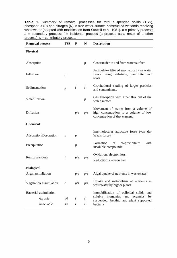
Generally, key processes responsible for pollutant removal in CWs are sedimentation,

chemical precipitation and adsorption, microbial activities and macrophyte uptake

(Vymazal 2001; Kadlec and Wallace 2009). Still, numerous factors affect the removal

processes and a pollutant is generally removed as a result of several interconnected

processes. In Table 1, the most common removal mechanisms for P, N and TSS are

listed. However, the removal mechamisms in CWs remain an active research area

(Gottschall et al. 2007; Kadlec and Wallace 2009), and therefore, the information

enclosed in Table 1 should not be taken as definate. The removal processes in wetlands

are very complex and which processes dominate depends to a great extent on

vegetation and water flow, factors that are relatively unexpensive and easy to

manipulate. Thus, more knowledge about how vegetation and water flow affects

pollutant removal may enable the design of low cost CWs that are optimized for

wastewater treatment.

Nitrogen removal in CWs is highly affected by both temperature and the level of

oxygen, whereas it is usually agreed that TSS and P removal processes, due to their

physical (sedimentation) and chemical (precipitation and adsorption) characteristics,

are not as sensitive to temperature effects. However, P removal can be significanly

affected by the oxygen status in the CW (Soto-Jimenez et al. 2003; Kadlec and

Wallace 2009). Also, on a seasonal level, differences in the removal of P can be seen

due to higher P uptake by vegetation during summer and lower during fall and winter.

Also, high returns of P from the decomposing vegetation litter during the fall may

counterbalance the high uptake rates during summer (Kadlec and Knight 1996).

5

Table 1. Summary of removal processes for total suspended soilds (TSS), phosphorus (P) and nitrogen (N) in free water surface constructed wetlands receiving wastewater (adapted with modification from Stowell et al. 1981). p = primary process; s = secondary process; i = incidental process (a process as a result of another process); c = contributory process.

Removal process TSS P N Description

Physical

Absorption

p Gas transfer to and from water surface

Filtration p

Particulates filtered mechanically as water

flows through substrate, plant litter and

roots

Sedimentation p i i Gravitational settling of larger particles

and contaminants

Volatilization p Gas absorption with a net flux out of the

water surface

Diffusion p/s p/s

Movement of matter from a volume of

high concentration to a volume of low

concentration of that element

Chemical

Adsorption/Desorption s p

Intermolecular attractive force (van der

Waals force)

Precipitation p Formation of co-precipitates with

insoluble compounds

Redox reactions i p/s p/s Oxidation: electron loss

Reduction: electron gain

Biological

Algal assimilation p/s p/s Algal uptake of nutrients in wastewater

Vegetation assimilation c p/s p/s Uptake and metabolism of nutrients in

wastewater by higher plants

Bacterial assimilation

Aerobic

Anaerobic

s/i

s/i

i

i

i

i

Immobilization of colloidal solids and

soluble inorganics and organics by

suspended, benthic and plant supported

bacteria

6

2.2.1 NITROGEN REMOVAL IN CONSTRUCTED WETLANDS

In CWs, nitrogen is removed via several pathways that may start with the decomposition of organic nitrogen present in wastewater by heterotrophic bacteria and fungi to ammonium (NH4

+), a process called ammonification (Fig. 1). This process may occur both in aerobic and anaerobic environments, but is much faster under the former condition. Also, ammonium may be temporarily removed from the water column by binding to negatively charged sites on soil particles in the CW sediment through adsorption (Mitsch and Gosselink 2000). However, changes in water chemistry or hydrology can release loosely bound NH4

+ back to the water column through desorption (Reddy and Patrick 1984). Still, removal of NH4

+ in CWs is dominated by an aerobic process called nitrification, in which NH4

+ is oxidized to nitrite (NO2

-) and further to nitrate (NO3-) by bacteria (Fig. 1). The nitrification rates in

a CW will be favored by oxic conditions, the availability of inorganic carbon and NH4

+, as well as temperature and pH ranges of 30–40°C and 7.5–8, respectively (Kadlec and Knight 1996). Nitrification may still occur at dissolved oxygen levels down to about 0.3 mg L-1 (Reddy and Patrick 1984). However, more recent studies have indicated that oxygen levels of 1–2 mg L-1 in CW water columns can decrease NH4

+ removal through lower nitrification rates (Hammer and Knight 1994; Okurut et al. 1999). Ammonium may also be lost to the atmosphere as ammonia gas (NH3) through a process called ammonia volatilization (Table 1; Fig. 1). However, at pH of below 8 and quiescent flow conditions, which are typical for CWs, volatilization is normally insignificant as a process for NH4

+ removal (Kadlec and Knight 1996).

Figure 1. A simplified illustration of the nitrogen cycle in free water surface constructed wetlands (modified from Kadlec and Knight 1996).

Diffusion may transfer NO3- from the CW water phase to the sediments and vice versa

(Fig. 1; Reddy and Patrick 1984). Nitrate is transformed by bacteria through a process called denitrification (Fig. 1) to nitrogen gas (N2), which diffuses from the CW water surface and thus returns nitrogen to the atmosphere.

NH4+

floc or sediment/soil

bottom level

NH4+

NH4+

NO3-

NO3-

NO3-

NO2-

NO3-

NO4

4+

3-

NONO2NO

NO- 3-

roots

Organic N

roots

Organic NOrganic N

roots

Organic N

NHNH

NH3 (gas) Air

water level

N2 + N2O (gases)

Organic NOrganic N

NH3 (gas)

7

The denitrifying bacteria are located on epiphytic biofilms that coat submerged CW

surfaces, which mainly are sediments, plant parts and litter (Bastviken et al. 2003).

Denitrification is favored by anoxic conditions, high availability of organic carbon,

high temperatures (optimum 60–75°C) and pH ranges of 6–8.5 (Reddy and Patrick

1984). The denitrification process means a one-way loss of nitrogen from a CW

system (Fig. 1).

The transfer of di-nitrogen gas (N2) from the atmosphere to nitrogen in the water phase

(a form of absorption) is a bacterial process called nitrogen fixation (Fig. 1). However,

nitrogen fixation is normally not significant in CWs receiving wastewater (Kadlec and

Knight 1996).

Assimilation of nitrogen, i.e. uptake of inorganic nitrogen and transformation to

organic nitrogen in living cells and tissues of plants, algae and microorganisms (Table

1), is considered to be insignificant in high-load CWs (Brix 1997; Kadlec 2005b).

Wetland macrophytes favor NH4+-N as the nutrient form of nitrogen since it is more

energy efficient as a building stone for amino acids, proteins and other nitrogenous

organic molecules (Kadlec and Knight 1996; Wetzel 2001). Still, macrophytes can also

take up NO3-, but the assimilation rate is determined by the NH4

+-N availability in the

CW (Martin and Reddy 1997). However, when vegetation dies, substantial amounts of

N are returned to the water and soil of the CW through decomposition and

mineralization (Nichols 1983; Howard-Williams 1985). Thus, CW vegetation is only

considered to be a temporary N sink, except if the biomass is harvested (Brix 1997).

Generally, FWS CWs with emergent vegetation treating wastewater of inlet

concentrations in the range 7.4–19 mg NH4+-N L

-1 can achieve relative removal of

incoming concentration in the order of 28–60% and an absolute removal of 0.18–1.51

g NH4+-N m

-2 day

-1 (Kadlec and Knight 1996; Kyambadde et al. 2005; Vymazal 2007).

2.2.2 PHOSPHORUS REMOVAL IN CONSTRUCTED WETLANDS

The key P fractions in a wastewater receiving CW are normally particulate phosphorus

(PP) and dissolved phosphorus (DP; Fig. 2), together comprising total P (TP).

Dissolved P, normally as phosphate-phosphorus (PO43-

-P), is available for living

organisms, whereas PP generally must go through transformations to become available

and further transformed to organic P (OP). Both abiotic and biotic processes control

the relative P fraction sizes and the transformation rates of P fractions within the CW

water column and sediment/soil. Abiotic processes include sedimentation, adsorption

to sediment/soils, precipitation, and exchange processes between soil/sediment and the

overlying water column. Biotic processes include assimilation by vegetation, plankton,

periphyton and microorganisms (Reddy et al. 1999; Table 1). Many researchers

consider accretion, i.e. the creation of new stable residuals, as the major long-term P

storage process in wetlands (Nichols 1983; Howard-Williams 1985; Richardson and

Marshall 1986; Reddy et al. 1999; Kadlec and Wallace 2009). The accretion process is

the sum of chemical P precipitation, adsorption and accumulation of detritus in the CW

sediment/soil.

8

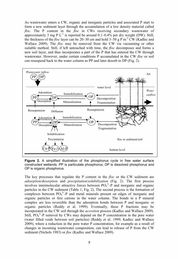
As wastewater enters a CW, organic and inorganic particles and associated P start to form a new sediment layer through the accumulation of a low density material called floc. The P content in the floc in CWs receiving secondary wastewater of approximately 3 mg P L-1 is reported be around 0.1–0.4% per dry weight (DW). Still, the thickness of the floc layer can be 20–30 cm and hold 3–50 g P m-2 CW (Kadlec and Wallace 2009). The floc may be removed from the CW via vacuuming or other suitable method. Still, if left untouched with time, the floc decomposes and forms a new soil layer, and thus incorporates a part of the P that has entered the CW through wastewater. However, under certain conditions P accumulated in the CW floc or soil can resuspend back to the water column as PP and later desorb to DP (Fig. 2).

Figure 2. A simplified illustration of the phosphorus cycle in free water surface constructed wetlands. PP is particulate phosphorus, DP is dissolved phosphorus and OP is organic phosphorus.

The key processes that regulate the P content in the floc or the CW sediment are adsorption/desorption and precipitation/solubilization (Fig. 2). The first process involves intermolecular attractive forces between PO4

3--P and inorganic and organic particles in the CW sediment (Table 1; Fig. 2). The second process is the formation of complexes between PO4

3--P and metal minerals present on edges of inorganic and organic particles or free cations in the water column. The bonds in a P mineral complex are less reversible than the adsorption bonds between P and inorganic or organic particles (Reddy et al. 1999). Eventually, these P fractions may be incorporated in the CW soil through the accretion process (Kadlec and Wallace 2009). Still, PO4

3--P removal by CWs may depend on the P concentration in the pore water (water filled voids between soil particles) (Reddy et al. 1999; Kadlec and Wallace 2009), where a reduction in the pore water P concentration, for example as a result of changes in incoming wastewater composition, can lead to release of P from the CW sediment (Nichols 1983) or floc (Kadlec and Wallace 2009).

Wastewater inflow

Water outflow

floc or sediment/soil

Immobilization

PP

OP

DP

Mineralization

Mineralization

Decomposition Fragmentation

Immobilization

Ca-P P Fe-P P Al-P

PP DP

PP DP Adsorption

OP

Desorption

Diffusion

PP Decomposition

Fragmentation

Resuspension

Soil accumulation

Resuspension

Soil accumulation

Adsorption

Desorption

Precipitation

Desorption

Solubilization

Desorption

water level

bottom level

roots

Air

9

Also, adsorption/desorption and precipitation/solubilization are controlled by factors

such as pH, redox potential and the amount of P and metal minerals in the sediment

(Kadlec and Wallace 2009). In CW environments with 6 < pH < 8, PO43-

-P can be

adsorbed to, and precipitate with, minerals of iron and aluminum present in the CW

sediment/soil (Richardson 1985; Gale et al. 1994; Lindstrom and White 2011). Still,

for iron rich sediments, aerobic conditions are also required for the P precipitation to

occur (Kadlec and Wallace 2009). The complex between PO43-

-P and calcium is not

sensitive to anoxic conditions (Kadlec and Wallace 2009), but requires CW

environments with pH > 8 for the precipitation to occur and remain stable (Nichols

1983; Reddy and D´Angelo 1994; Reddy et al. 1999).

Several studies have declared that P removal by CWs normally decreases with time

and discussed that this could be because most sorption sites on the metal minerals

present in the soil have become saturated (Richardson 1985; Okurut et al. 1999;

Kadlec 2005a). This behaviour may be referred to as the “aging phenomena” in

wetlands (Kadlec 1984). As a consequence of the “aging phenomena”, the

sediment/soil can start to leak P (Nichols 1983; Richardson 1985; Kadlec and Knight

1996). However, leakage of P from newly created CWs has also been observed due to

lower P concentrations in incoming water to the CW than historical P concentration on

the site (Kadlec and Wallace 2009). Also, a change from oxic to predominantly anoxic

surroundings in the CW sediment can cause solubilization of P bound to iron minerals

in the wetland soil (Fig. 2; Gale et al. 1994; Vymazal 2001; Soto-Jimenez et al. 2003;

Kadlec and Wallace 2009). Thus, adsorption and precipitation of P by CW

sediment/soils is not necessary stable, but instead reversible. The only mechanism to

ultimately remove P from the CW is via dredging of the sediment/soil for ultimate

disposal (Stowell et al. 1981) or by harvesting the CW macrophytes (Brix 1997).

However, Lindstrom and White (2011) suggested that aluminum sulfate (alum)

addition could be a more cost effective method to improve P removal in aging CWs.

Still, studies have suggested that P precipitated with aluminum chemicals is of low P

fertilization value and could, if applied to agricultural fields, result in P accumulations

in soils with potential environmental risks associated to surface runoff of P (Ippolito et

al. 2002; Krogstad et al. 2005).

Phosphorus is a limiting element for growth of algae and macrophytes in CWs, and

thus, these organisms effectively assimilate P from wastewater present in CWs.

However, a part of the assimilated P is returned to the water phase upon senescence

and succeeding decomposition, but may also be incorporated into new CW sediments

and finally accreted (Kadlec and Wallace 2009). The net effect of macrophytes on the

water phase P concentration may depend on macrophyte age and climatic conditions,

but also on the CW operation and maintenance (Kadlec 2005a).

Literature shows that FWS CWs with emergent vegetation treating wastewater with

inlet concentrations in the range 3.7–24 mg TP L-1

achieve variable relative removal of

incoming concentration in the order of 9–62% and an absolute removal ranging

between 0.02–2.14 g TP m-2

day-1

(Kadlec and Knight 1996; Greenway and Woolley

1999; Kyambadde et al. 2005; Diemont 2006; Vymazal 2007).

10

2.2.3 SUSPENDED SOLIDS REMOVAL IN CONSTRUCTED WETLANDS

Removing suspended solids (SS) in wastewater is important since it prevents silting

and also removes nutrients masses (attached to solids) reaching down-stream water

bodies. Generally, removal of SS is not affected by temperature (Kadlec 2003; Kadlec

and Wallace 2009) indicating that abiotic factors dominate the removal processes. The

key variables for SS removal in CWs are adequate time for settling combined with

trapping in the litter, sediment and soil. The relatively slow flow in CWs is often

enough to give time for physical settling of SS, and at a constant flow, macrophytes

may effectively contribute to increased sedimentation (Braskerud 2001).

Macrophytes may also limit resuspension of the sedimented particles by trapping these

in the litter layer (Kadlec and Wallace 2009). Still, fragmentation of detritus from

macrophytes and algae can produce particulate matter and thus increase SS

concentration in a CW. Also, bioturbation by fish and mammals, water shear and gas

flotation by oxygen or methane can resuspend solids into the CW water column. In

addition, a weak seasonal dynamic in TSS removal may occur in CWs through algae

and macrophytic turnover rates (Kadlec and Wallace 2009).

Based on numerous CW studies, Kadlec and Knight (1996) proposed a rule of thumb

which stated that about 75% of incoming TSS is removed if inflow concentrations of

TSS are above 20 mg L-1

. The absolute removal of TSS in FWS CWs with emergent

vegetation may be in the order of 2–10 g TSS m-2

day-1

depending on the TSS mass

loading rates (Kadlec and Wallace 2009).

11

2.3 CRITICAL FACTORS FOR POLLUTANT REMOVAL

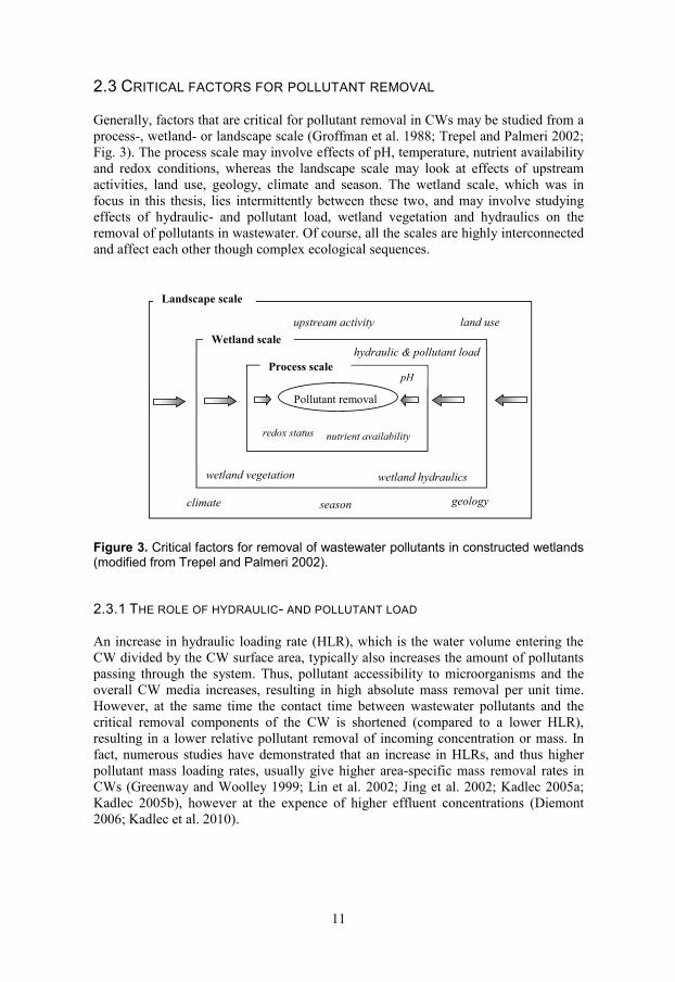
Generally, factors that are critical for pollutant removal in CWs may be studied from a process-, wetland- or landscape scale (Groffman et al. 1988; Trepel and Palmeri 2002; Fig. 3). The process scale may involve effects of pH, temperature, nutrient availability and redox conditions, whereas the landscape scale may look at effects of upstream activities, land use, geology, climate and season. The wetland scale, which was in focus in this thesis, lies intermittently between these two, and may involve studying effects of hydraulic- and pollutant load, wetland vegetation and hydraulics on the removal of pollutants in wastewater. Of course, all the scales are highly interconnected and affect each other though complex ecological sequences.

Figure 3. Critical factors for removal of wastewater pollutants in constructed wetlands (modified from Trepel and Palmeri 2002).

2.3.1 THE ROLE OF HYDRAULIC- AND POLLUTANT LOAD

An increase in hydraulic loading rate (HLR), which is the water volume entering the CW divided by the CW surface area, typically also increases the amount of pollutants passing through the system. Thus, pollutant accessibility to microorganisms and the overall CW media increases, resulting in high absolute mass removal per unit time. However, at the same time the contact time between wastewater pollutants and the critical removal components of the CW is shortened (compared to a lower HLR), resulting in a lower relative pollutant removal of incoming concentration or mass. In fact, numerous studies have demonstrated that an increase in HLRs, and thus higher pollutant mass loading rates, usually give higher area-specific mass removal rates in CWs (Greenway and Woolley 1999; Lin et al. 2002; Jing et al. 2002; Kadlec 2005a; Kadlec 2005b), however at the expence of higher effluent concentrations (Diemont 2006; Kadlec et al. 2010).

Pollutant removal

Process scale

geology climate

wetland vegetation wetland hydraulics

hydraulic & pollutant load

pH

redox status

season

land use

nutrient availability

Wetland scale upstream activity

Landscape scale

12

Lin et al. (2002) described increased absolute mass removal of P ranging from 0.06 to

0.14 g m-2

day-1

and for NH4+-N from 0.04 to 0.09 g m

-2 day

-1 with increasing HLRs

(18–68 mm day-1

) in a planted FWS CW receiving aquaculture wastewater.

Nevertheless, at the highest HLR (135 mm day-1

) the removal rates decreased to 0.12 g

P m-2

day-1

and 0.08 g NH4+-N m

-2 day

-1, proposing that there could be an optimal

level of HLR to achieve maximum pollutant removal. Also, Jing et al. (2002) reported

increased absolute mass removal rate of PO4-3

and NH4+-N with increasing mass

loading rates for CWs operating at a hydraulic residence time (HRT) of 2 to 4 days.

Still, at a HRT of 1 day (HLR of 120 mm day-1

) mass removal rates decreased

noticeably, which the authors concluded was an effect of insufficient time for removal

processes to occur. However, Lin et al. (2002) and Jing et al. (2002) applied the

different HLRs to the same CW system subsequently, thus possibly introducing

interpretation problems due to effects such as the “aging phenomena” as described by

Kadlec (1984), which may cause exhaustion of the CW sediment P and NH4+-N

adsorption capacity. Also, the development of anaerobic conditions in the CW

sediment/soil due to accumulation of dead plant material during the experiment could

cause solubilization of P precipitates and lower nitrification rates. Also, the studied

CWs were microcosms, thus, increasing the risk for not adequately imitating the

realistic environmental conditions. Hence, incorrect conclusions about the most

favorable HLR giving maximum mass removal in the CWs could have been made by

Lin et al. (2002) and Jing et al. (2002). Still, Martín et al. (2013) studied the effect of

different HLRs ranging from 19 to 130 mm day-1

, which were applied subsequently to

a large FWS CWs (9 ha) over a period of 2 years. Results from the cited study showed

that removal of TP (0.0031–0.025 g m-2

day-1

) and TSS (0.344–2.41 g m-2

day-1

)

increased with increasing HLR, without any noted decrease at the highest HLR (which

was applied last). Still, the TP mass loading rates were somewhat lower than in Lin et

al. (2002) and Jing et al. (2002) which could have affected the level of achieved

“aging”. Nevertheless, despite the large body of research, at present a broad

generalization of finding optimum HLR for achieving maximum pollutant removal in

CWs is not possible. Ultimately, the CW designer has to decide whether certain

concentration criteria are to be met or a high mass removal is desired. Moreover,

nutrient mass load to a CW may also strongly affect macrophyte nutrient uptake rates

and thus regulate the amount of nutrients that can be removed via macrophyte

harvesting (Kadlec and Wallace 2009). In more detail, nutrient concentration of several

emergent macrophyte species, show increasing tissue P with increasing P load,

stretching from 0.05–0.5% P per DW biomass (Kadlec and Wallace 2009). Also,

normally, macrophyte standing crop (total amount of dead or living biomass found at

any given moment in a CW) increases with increasing P load, extending from about

1000 g DW biomass m-2

(low nutrient availability) to 6000 g DW biomass m-2

(high

nutrient availability; Kadlec 2005a).

2.3.2 THE ROLE OF WETLAND VEGETATION

Generally, rooted emergent macrophytes assist pollutant removal in CWs through both

indirect and direct mechanisms. The indirect mechanisms are related to physiological,

morphological and biogeochemical factors aided by macrophytes to the CW matrix.

13

More specifically, macrophytes may indirectly facilitate removal processes by

providing surfaces for active and diverse microbial communities (Eriksson and

Weisner 1996; Eriksson and Andersson 1999; Bastviken et al. 2003; Rossmann et al.

2012), by preventing resuspension of sedimented pollutants (Braskerud 2001) and

supplying oxygen to the CW soil (Reddy et al. 1989; Sorrell and Armstrong 1994; Brix

1997). The latter process occurs via aerenchymatous stem tissue which transports

oxygen to roots rhizomes from where the oxygen may eventually diffuse to the CW

sediment and pore water. Thus, it is not surprising that numerous studies performed on

the CW scale, that have compared non-vegetated with vegetated CWs, report

significantly higher removal of wastewater pollutants in the latter systems, and that

even macrophyte species can be of significance (Klomjek and Nitisoravut 2005;

Diemont 2006; Yang et al. 2007; Brisson and Chazarenc 2009; Rossmann et al. 2012;

Gagnon et al. 2012).

The direct pollutant removal mechanism provided by macrophytes is the assimilation

of nutrients from wastewater into the macrophytic biomass. Looking at P, Kadlec

(2005a) states that only 10–20% of the assimilate P is permanently stored as residuals

from decomposition processes while the rest is returned to the system upon vegetation

senescence (Kadlec 2005a). Thus, the only way to ultimately remove P trapped in the

macrophytic biomass is through harvesting. For temperate climates, Kadlec (2005a)

stated that macrophyte uptake in emergent FWS CWs was between 0.0014 and 0.055 g

P m-2

day-1

and suggested that 20% of the uptake could be considered as a net removal

achieved through above-ground biomass harvesting. This gives a net removal of P via

harvesting of less than 0.011 g P m-2

day-1

for emergent FWS CWs in temperate

climates. However, higher macrophyte uptake rates have been reported for tropical

CWs receiving wastewater. Okurut (2001) reported that Cyperus papyrus L. growing

in CWs receiving 0.26 g P m-2

day-1

had an uptake rate of 0.024 g P m-2

day-1

.

Kyambadde et al. (2004) stated uptake rates by C. papyrus of 0.090 g P m-2

day-1

at a

load of 0.62 g PO43-

-P m-2

day-1

. Later, Kyambadde et al. (2005) demonstrated even

higher P uptake rates by C. papyrus in the order of 0.18 g P m-2

day-1

at a load of 2.2 g

PO43-

-P m-2

day-1

. Thus, the amount of area-specific P removed via harvesting of

tropical CWs could be considerably higher than that reported by Kadlec (2005a). This

is not surprising since the above-ground biomass of various macrophytes grow and die

at quicker cycles in tropical climates compared the single annual growing season in

northern climates (Reddy et al. 1999). Also, the seasonal translocations of nutrients

from above-ground to below-ground macrophyte parts are less pronounced in tropical

regions (Vymazal 2007) which creates the possibility to implement CW management

strategies that include multiple harvests per year. This type of management technique

in CWs can possibly play a significant role for the removal and reclamation route for

nutrients in wastewater.

Nevertheless, the literature contains conflicting data about the significance of emergent

macrophytes as nutrient traps in wastewater receiving CWs. Generally, harvesting

macrophytes for nutrient removal is not valued as significant due to the poor nutrient

uptake rates by macrophytes when related to the high nutrient loads normally found in

wastewater treating CWs (Brix 1997; Kadlec 2005a; Kadlec 2005b). Looking at P,

generally, less than 10% of the P loaded to CWs can be found in harvested biomass

(Kim and Geary 2001; Okurut 2001; Toet et al. 2005; Kyambadde et al. 2005). Still,

when relating the P found in macrophytic biomass to the total removal of P by a FWS

CW a different picture emerges.

14

Studies from tropical CWs have reported that the fraction of total P removal by

emergent macrophyte can be in the order of 35–90% of the total P removed by a CW if

the macrophytes are at an exponential growth stage (Okurut 2001; Kyambadde et al.

2004). Still, some explanations for the high macrophyte uptake rates reported by

Kyambadde et al. (2005) and Kyambadde et al. (2004), other than the tropical

conditions, could be the substrate-free design and the fact that the plants were only 7 to

8 months old at the end of the studies.

The lower macrophyte uptake rates reported by Okurut (2001) compared to the ones

obtained by Kyambadde et al. (2005) were most likely related to lower mass load into

the CWs in the former study. Also, in the study by Okurut (2001) higher macrophyte

age and thus the senescent stage of the macrophytes at the end of the 18 months long

study period may have resulted in lower macrophyte P uptake. Still, Martín et al.

(2013) reported that P accumulated in above-ground biomass of macrophytes growing

in FWS CWs in Spain represented around 20% of the total P removed by the system

during at the end of a 2 year study period. In the cited study, macrophyte P uptake after

a 2 year growing period was 0.019 g P m-2

day-1

. Thus, studies show that macrophyte P

uptake may be a major component of total P removal by CWs and that macrophyte

growth stage (age) may be an important factor for the assessment of macrophyte

nutrient uptake in relation to overall CW mass load and removal.

Correct vegetation management is critical for achieving sustainable optimal water

treatment functions in CWs (Thullen et al. 2005). This may not be surprising since

macrophyte turnover rates in aquatic ecosystems can augment bioavailable P to the

water column (Hansson and Granéli 1984) and thereby influence overall nutrient

removal in CWs in a negative way (Lü et al. 2012). Many researchers have signified

the importance of regular macrophyte harvesting in CWs to achieve efficient removal

of nutrients from wastewater (DeBusk and Ryther 1987; Okurut 2001; Kyambadde et

al. 2005; Bojcevska 2007; Vymazal 2007; Borin and Salvato 2012; Hoffmann et al.

2012). Still, Martín et al. (2013) reported a period of degraded water quality after

macrophyte harvest. Nevertheless, regular and proper harvesting methods may keep

macrophytes at optimum growth stage and thus ensure optimal nutrient uptake

(Vymazal 2007), since P concentrations in above-ground macrophyte biomass declines

with increasing growing time. This decline can be substantial, i.e. for Phragmites

australis (Cav.) Steud., per cent P of DW biomass can be 0.47% at day 30 and

decrease to 0.17% at day 180 of growth (Kadlec and Wallace 2009). Thus, an efficient

harvesting frequency may also aid in the maintenance of a high quality standing crop

of young and actively growing macrophyte shoots. This way, nutrient uptake and

storage by macrophytes growing in CWs can be nearly continuous and represent a

significant route for nutrient removal from wastewater. Also, through harvest, vital

nutrients such as phosphorus may be recycled as fertilizers, decreasing the need for

mined phosphorus, which is not a sustainable source of this vital nutrient when looking

at long-term geological, economic and geopolitical aspects (Elser 2012). Thus, for

developing countries, the harvested biomass could represent a valuable resource for

local communities (Abila 1998; Gichuki et al. 2001).

In a review of 35 studies on effects of macrophyte species on removal efficiency in

CWs, Brisson and Chazarenc (2009) concluded that species identity does matter, but

that making well-founded recommendations for species selection was difficult.

15

Okurut et al. (1999) and Kyambadde et al. (2005) reported that CWs planted with C.

papyrus displayed significantly higher area-specific mass removal rates of NH4+-N

than those planted with other macrophyte species.

Additionally, characteristics in macrophyte structures could influence nitrification

rates and thus removal of NH4+-N in CWs. Eriksson and Andersson (1999) reported

that the biofilm nitrification varied greatly between litter of different macrophytes and

suggested that the difference in biofilm nitrification among the species was a result of

differences in the physical and chemical characteristics of the litter. In addition,

substances released from the decomposing macrophytes could have an inhibiting effect

on the nitrifying bacteria and their activity which in turn may promote more or less

biofilm development and hence also nitrifying bacteria (Bastviken et al. 2003).

16

2.3.3 THE ROLE OF WETLAND HYDRAULICS

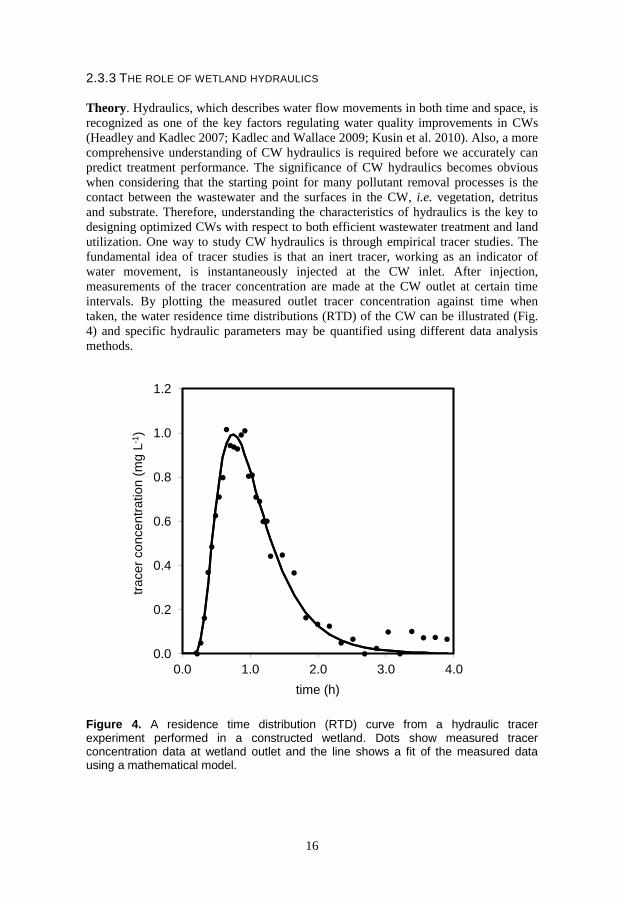
Theory. Hydraulics, which describes water flow movements in both time and space, is

recognized as one of the key factors regulating water quality improvements in CWs

(Headley and Kadlec 2007; Kadlec and Wallace 2009; Kusin et al. 2010). Also, a more

comprehensive understanding of CW hydraulics is required before we accurately can

predict treatment performance. The significance of CW hydraulics becomes obvious

when considering that the starting point for many pollutant removal processes is the

contact between the wastewater and the surfaces in the CW, i.e. vegetation, detritus

and substrate. Therefore, understanding the characteristics of hydraulics is the key to

designing optimized CWs with respect to both efficient wastewater treatment and land

utilization. One way to study CW hydraulics is through empirical tracer studies. The

fundamental idea of tracer studies is that an inert tracer, working as an indicator of

water movement, is instantaneously injected at the CW inlet. After injection,

measurements of the tracer concentration are made at the CW outlet at certain time

intervals. By plotting the measured outlet tracer concentration against time when

taken, the water residence time distributions (RTD) of the CW can be illustrated (Fig.

4) and specific hydraulic parameters may be quantified using different data analysis

methods.

Figure 4. A residence time distribution (RTD) curve from a hydraulic tracer experiment performed in a constructed wetland. Dots show measured tracer concentration data at wetland outlet and the line shows a fit of the measured data using a mathematical model.

0.0

0.2

0.4

0.6

0.8

1.0

1.2

0.0 1.0 2.0 3.0 4.0

tra

ce

r co

nce

ntr

atio

n (

mg L

-1)

time (h)

17

The basic hydraulic parameters encountered in the CW literature are the mean (tm) and

variance ( 2 ) of the RTD. The tm parameter indicates the average residence time of

water in the CW and 2 proposes the degree of water dispersion (Fogler 2006).

The tm-value may be related to the theoretical or nominal residence time, tn-value

(defined as the theoretical CW volume divide by the flow) to quantify the effective or

“active” CW volume (Thackston et al. 1987) as in Eq. (1)

sys

effective

n

m

V

V

t

te (1)

where e = effective CW volume ratio (-), Vsys = theoretical CW volume (m3) and

Veffective = total effective CW volume (m3) derived via tracer data. If e = 1 this indicates

that the entire CW volume is active in pollutant removal, i.e. 100% effective volume.

However, numerous studies show that e-values of CWs usually are in the range of 0.20

to 0.98 with a typical mean value of 0.82 (±0.8 SD) for FWS CWs (Kadlec and

Wallace 2009). Interestingly, e-values higher than 1 have also been reported in the

literature and have mainly been associated to flaws in water flow measurements during

the tracer experiment or estimations of the theoretical CW volume (Kadlec 1994a;

Kjellin et al. 2007).

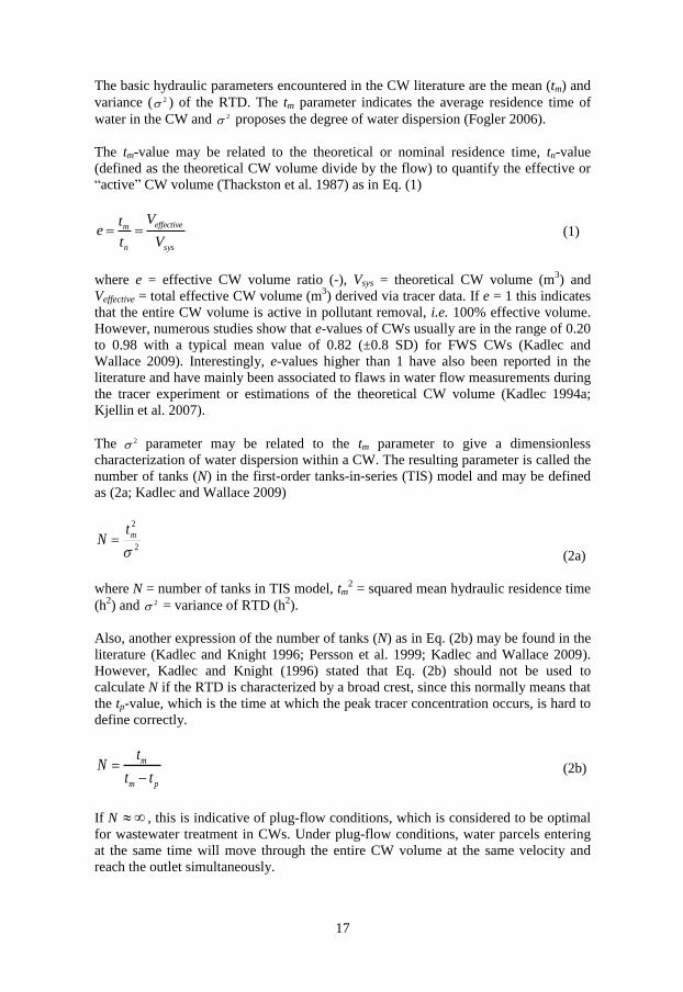
The 2 parameter may be related to the tm parameter to give a dimensionless

characterization of water dispersion within a CW. The resulting parameter is called the

number of tanks (N) in the first-order tanks-in-series (TIS) model and may be defined

as (2a; Kadlec and Wallace 2009)

2

2

mtN (2a)

where N = number of tanks in TIS model, tm2 = squared mean hydraulic residence time

(h2) and 2 = variance of RTD (h

2).

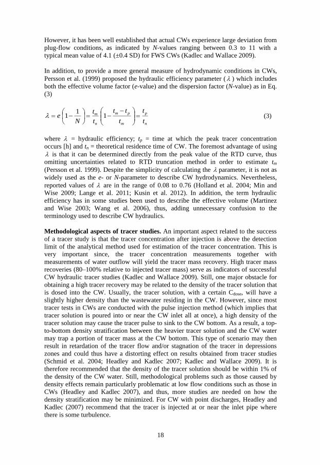
Also, another expression of the number of tanks (N) as in Eq. (2b) may be found in the

literature (Kadlec and Knight 1996; Persson et al. 1999; Kadlec and Wallace 2009).

However, Kadlec and Knight (1996) stated that Eq. (2b) should not be used to

calculate N if the RTD is characterized by a broad crest, since this normally means that

the tp-value, which is the time at which the peak tracer concentration occurs, is hard to

define correctly.

pm

m

tt

tN

(2b)

If N , this is indicative of plug-flow conditions, which is considered to be optimal

for wastewater treatment in CWs. Under plug-flow conditions, water parcels entering

at the same time will move through the entire CW volume at the same velocity and

reach the outlet simultaneously.

18

However, it has been well established that actual CWs experience large deviation from

plug-flow conditions, as indicated by N-values ranging between 0.3 to 11 with a

typical mean value of 4.1 (±0.4 SD) for FWS CWs (Kadlec and Wallace 2009).

In addition, to provide a more general measure of hydrodynamic conditions in CWs,

Persson et al. (1999) proposed the hydraulic efficiency parameter ( ) which includes

both the effective volume factor (e-value) and the dispersion factor (N-value) as in Eq.

(3)

n

p

m

pm

n

m

t

t

t

tt

t

t

Ne

1

11 (3)

where = hydraulic efficiency; tp = time at which the peak tracer concentration

occurs [h] and tn = theoretical residence time of CW. The foremost advantage of using

is that it can be determined directly from the peak value of the RTD curve, thus

omitting uncertainties related to RTD truncation method in order to estimate tm

(Persson et al. 1999). Despite the simplicity of calculating the parameter, it is not as

widely used as the e- or N-parameter to describe CW hydrodynamics. Nevertheless,

reported values of are in the range of 0.08 to 0.76 (Holland et al. 2004; Min and

Wise 2009; Lange et al. 2011; Kusin et al. 2012). In addition, the term hydraulic

efficiency has in some studies been used to describe the effective volume (Martinez

and Wise 2003; Wang et al. 2006), thus, adding unnecessary confusion to the

terminology used to describe CW hydraulics.

Methodological aspects of tracer studies. An important aspect related to the success

of a tracer study is that the tracer concentration after injection is above the detection

limit of the analytical method used for estimation of the tracer concentration. This is

very important since, the tracer concentration measurements together with

measurements of water outflow will yield the tracer mass recovery. High tracer mass

recoveries (80–100% relative to injected tracer mass) serve as indicators of successful

CW hydraulic tracer studies (Kadlec and Wallace 2009). Still, one major obstacle for

obtaining a high tracer recovery may be related to the density of the tracer solution that

is dosed into the CW. Usually, the tracer solution, with a certain Cdose, will have a

slightly higher density than the wastewater residing in the CW. However, since most

tracer tests in CWs are conducted with the pulse injection method (which implies that

tracer solution is poured into or near the CW inlet all at once), a high density of the

tracer solution may cause the tracer pulse to sink to the CW bottom. As a result, a top-

to-bottom density stratification between the heavier tracer solution and the CW water

may trap a portion of tracer mass at the CW bottom. This type of scenario may then

result in retardation of the tracer flow and/or stagnation of the tracer in depressions

zones and could thus have a distorting effect on results obtained from tracer studies

(Schmid et al. 2004; Headley and Kadlec 2007; Kadlec and Wallace 2009). It is

therefore recommended that the density of the tracer solution should be within 1% of

the density of the CW water. Still, methodological problems such as those caused by

density effects remain particularly problematic at low flow conditions such as those in

CWs (Headley and Kadlec 2007), and thus, more studies are needed on how the

density stratification may be minimized. For CW with point discharges, Headley and

Kadlec (2007) recommend that the tracer is injected at or near the inlet pipe where

there is some turbulence.

19

Therefore, especially in CWs which normally experience little turbulence at the inlet, it

may be crucial to ensure that the tracer injection method is properly performed. Also,

the injection time should not exceed more than a few per cent of the CW´s tn-value.

Thus, by proper preparations and planning, low tracer mass recoveries and thus

uncertain hydraulic results may be avoided.

Therefore, considering the potential importance of the injection method, it is

unfortunate that many published CW salt tracer studies give insufficient details about

the injection methods used (Dal Cin and Bendoricchio 2002; Persson 2005; Dierberg

and DeBusk 2005; Ronkanen and Kløve 2007; Speer et al. 2009). There is very little

research related to effects of salt tracer injection methods on tracer behaviour and

subsequent tracer mass recovery. Especially for FWS CWs, interaction effects of tracer

injection technique and different types of vegetation on tracer recoveries and

subsequent hydraulic results have received very little attention. Given the general

agreement among researchers about the impact of vegetation for CW hydraulics, it is

surprising that such interaction effects are left essentially unstudied.

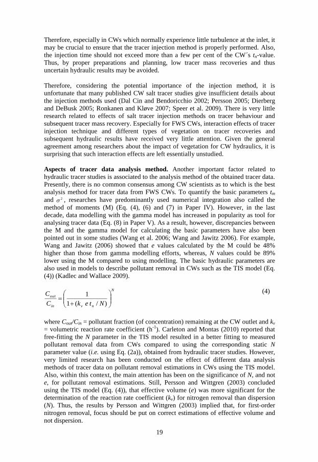
Aspects of tracer data analysis method. Another important factor related to

hydraulic tracer studies is associated to the analysis method of the obtained tracer data.

Presently, there is no common consensus among CW scientists as to which is the best

analysis method for tracer data from FWS CWs. To quantify the basic parameters tm

and 2 , researches have predominantly used numerical integration also called the

method of moments (M) (Eq. (4), (6) and (7) in Paper IV). However, in the last

decade, data modelling with the gamma model has increased in popularity as tool for

analysing tracer data (Eq. (8) in Paper V). As a result, however, discrepancies between

the M and the gamma model for calculating the basic parameters have also been

pointed out in some studies (Wang et al. 2006; Wang and Jawitz 2006). For example,

Wang and Jawitz (2006) showed that e values calculated by the M could be 48%

higher than those from gamma modelling efforts, whereas, N values could be 89%

lower using the M compared to using modelling. The basic hydraulic parameters are

also used in models to describe pollutant removal in CWs such as the TIS model (Eq.

(4)) (Kadlec and Wallace 2009).

(4)

where Cout/Cin = pollutant fraction (of concentration) remaining at the CW outlet and kv

= volumetric reaction rate coefficient (h-1

). Carleton and Montas (2010) reported that

free-fitting the N parameter in the TIS model resulted in a better fitting to measured

pollutant removal data from CWs compared to using the corresponding static N

parameter value (i.e. using Eq. (2a)), obtained from hydraulic tracer studies. However,

very limited research has been conducted on the effect of different data analysis

methods of tracer data on pollutant removal estimations in CWs using the TIS model.

Also, within this context, the main attention has been on the significance of N, and not

e, for pollutant removal estimations. Still, Persson and Wittgren (2003) concluded

using the TIS model (Eq. (4)), that effective volume (e) was more significant for the

determination of the reaction rate coefficient (kv) for nitrogen removal than dispersion

(N). Thus, the results by Persson and Wittgren (2003) implied that, for first-order

nitrogen removal, focus should be put on correct estimations of effective volume and

not dispersion.

N

nvin

out

NtekC

C

)/(1

1

20

Factors affecting wetland hydraulics. Effect on CW hydraulics has mainly been

studied by varying the vegetation layout (Persson et al. 1999; Jenkins and Greenway

2005; Kjellin et al. 2007; Keefe et al. 2010), the location of inlet and outlet (Persson et

al. 1999), the CW bottom topography (Kjellin et al. 2007; Lightbody et al. 2007), the

CW shape (Persson 2000; Wörman and Kronnäs 2005) and the water depth (Holland et

al. 2004). However, there is a lack of studies comparing the effect of different types or

species of CW macrophytes and/or inlet water flow rates on CW hydraulics. Therefore,

in the present thesis, these two factors were chosen as methods to learn more about

CW hydraulics.

Vegetation. Vegetation in CWs may affect water flow patterns and velocities both on a

large scale and on a small scale The large scale effects have to do with the heterogenic

distribution and density of vegetation stands, which may produce short-circuiting paths

and dead zones i.e. zones that are not part of the main flowing CW volume (Persson et

al. 1999; Dal Cin and Persson 2000; Jenkins and Greenway 2005), whereas the small

scale effects are the results of shear dispersion against individual vegetation stems and

eddies formed around immersed stems (Kutija and Hong 1996; Nepf 1999). Kjellin et

al. (2007) showed that vegetation was the factor that most dominated the shape of

RTDs obtained from tracer experiments. The cited authors could thus show that

vegetation patterns controlled most of the water flow paths and argued that the

construction of wetlands should prioritize vegetation establishment more than the

design of bottom topography. Also, Keefe et al. (2010) reported better hydraulic

performance at the start of the vegetation growing season but observed short-circuiting

at the end of the growing season related to senescing vegetation. Also, studies have

shown that an increase in fringing emergent vegetation may result in decreased

effective volume and increased dispersion in CWs (Persson et al. 1999; Dal Cin and

Persson 2000).

Inlet flow rate. Changes in inlet flow rate may affect CW hydraulics by changing the

water velocities and promoting more or less dispersion. Holland et al. (2004) found a

decrease in dispersion and increase in hydraulic efficiency when the inlet flow rate in a

250 m2 FWS CW was raised by a factor of 2.7. Wanko et al (2010) also found that the

dispersion decreased when the flow rate into small (7.1 m2) CWs was increased by a

factor of 1.9. None of these two studies, however, provided statistically significant

results but nevertheless indicated that flow rate may play a greater role under naturally

pulsed conditions in CWs where there is a larger difference between the flow rates

(larger than a factor of 2.7). Nevertheless, Boutilier et al. (2011) reported that high

flow conditions caused flow channeling or short circuiting within a 100 m2 outdoor

situated wastewater treatment FWS CW. However, studies on the effect of flow rate on

FWS CW hydraulics are still scarce. Thus, more tracer experiments are needed,

especially in CW systems experiencing natural flow events, such as those in tropical

regions.

Can hydraulics affect pollutant removal in CWs? So far, there is a lack of empirical

studies that have simultaneously investigated both FWS CW hydraulics and

wastewater treatment performance. Still, those few studies that exist have reported that

hydraulics can affect in pollutant removal (Dierberg et al. 2005; Wang et al. 2006;

Boutilier et al. 2008; Boutilier et la. 2011).

21

Dierberg et al. (2005) studied the impact of short-circuiting paths characterized by

sparse populations of submerged aquatic vegetation (SAV) on P removal in a 147 ha

large FWS CW in Florida. The cited study found that relative removal of TP were

generally lower within short-circuited and deeper flow paths with sparse SAV

compared to flow paths with more dense SAV and shallower depth. However,

Dierberg et al. (2005) stated that it was not known how much of the low P removal

was caused by the shorter HRT and how much could be related to decrease in

biological activity as a result of the sparse SAV.

Boutilier et al. (2008) suggested that dispersion highly impacted the mass transport

processes within a 7 m2 FWS CW and that long-term operation of FWS CWs may

cause reduced HRTs and pollutant removal efficiency due to channeling (short-

circuiting). Boutilier et al. (2011) also suggested that channelling within a 100 m2

FWS CW could affect bacteria removal due to reduced HRTs and that the channelling

may have been caused by a combination of high flow conditions and dense cattail

population.

22

3. OBJECTIVES

The overall objective of the present thesis was to study critical factors affecting

wastewater treatment in FWS CWs receiving point-source wastewater. Research

findings were aimed to increase knowledge about proper guidelines for CW design,

operation and maintenance. Selected critical factors were CW vegetation and

hydraulics, but also hydraulic-and pollutant mass load. The factors were all generally

studied on the wetland scale (Fig. 3). However, season also became a factor, since

some of the studies were performed in tropical CWs, which are influenced by

pronounced periods of rain and drought. Moreover, data analysis method as a factor

for interpreting CW hydraulics and pollutant removal was investigated (a factor not

considered in Fig. 3). Studies were performed in Kenya and Sweden, in small (around

40-60 m2) FWS CWs and were of both empirical and simulated character. The doctoral

project resulted in five manuscripts (Table 2).

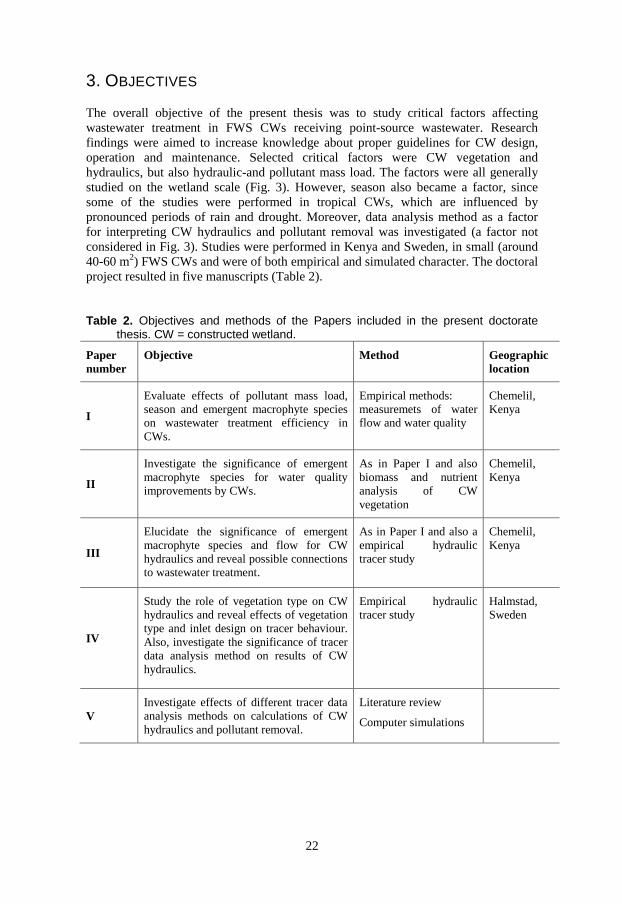
Table 2. Objectives and methods of the Papers included in the present doctorate thesis. CW = constructed wetland.

Paper

number

Objective Method Geographic

location

I

Evaluate effects of pollutant mass load,

season and emergent macrophyte species

on wastewater treatment efficiency in

CWs.

Empirical methods:

measuremets of water

flow and water quality

Chemelil,

Kenya

II

Investigate the significance of emergent

macrophyte species for water quality

improvements by CWs.

As in Paper I and also

biomass and nutrient

analysis of CW

vegetation

Chemelil,

Kenya

III

Elucidate the significance of emergent

macrophyte species and flow for CW

hydraulics and reveal possible connections

to wastewater treatment.

As in Paper I and also a

empirical hydraulic

tracer study

Chemelil,

Kenya

IV

Study the role of vegetation type on CW

hydraulics and reveal effects of vegetation

type and inlet design on tracer behaviour.

Also, investigate the significance of tracer

data analysis method on results of CW

hydraulics.

Empirical hydraulic

tracer study

Halmstad,

Sweden

V

Investigate effects of different tracer data

analysis methods on calculations of CW

hydraulics and pollutant removal.

Literature review

Computer simulations

23

4. METHODS

4.1 STUDY SITES AND EXPERIMENTAL DESIGNS

Studies in Paper I–III were performed in a FWS CW system in western Kenya,

receiving pre-treated sugar factory wastewater. The CW system consisted of eight

wetlands, each approximately 3 m x 20 m (Fig. 1 in Paper I). Four of the CWs were

planted with C. papyrus and four with Echinochloa pyramidalis (Lam.) Hitche and

Chase, both rooted emergent macrophytes. After treatment in the CW system, the

water was discharged into the Mbogo River which discharges to Lake Victoria. From

April 2004 to April 2005, the HLR was approximately 75 mm day-1

(HRT = 5.3 days)

in CWs 1–4 and 225 mm day-1

in CWs 5–8 (HRT = 1.8 days). From January to March

2006 the load was reduced to 45 mm day-1

(HRT = 8.2 days) in CWs 1–4 and 110 mm

day-1

in CWs 5–8 (HRT = 3.4 days). The mean water depth and mean volume during

April 2004 to April 2005 were 0.40 m (± 0.03 S.D.) and 24.5 m3 (± 3.2 S.D.), whereas,

during January to March 2006 the mean depth and mean volume were 0.33 m (± 0.03

S.D.) and 18.5 m3 (± 2.0 S.D.) for all eight CWs. Due to the possible impact of the

rainy and dry seasons, collected data was summarized and analyzed per season: period

1, short rains (19 November to 31 December 2004); period 2, dry season (1 January to

9 March 2005); period 3, long rains (10 March to 4 April 2005); and period 4, dry

season (19 January to 7 March 2006). Above-ground parts of the macrophytes were

harvested on three occasions: September 2004 (macrophytes had been growing for 21

months), April 2005 and December 2005. The macrophytes shoots were thus between

2–4 months old in period 1, 4–6 months in period 2, 7 months in period 3 and 1–2

months in period 4.

The study of Paper IV was performed in an experimental FWS CW system (Fig. 1a in

Paper IV), near Halmstad, Sweden. This system consisted of 18 rectangular pilot-scale

CW cells each with a ground surface area of 40 m2 and flat bottom area of 12 m

2 (Fig.

1b in Paper IV). The experimental design in Paper IV involved six CWs with free

vegetation development (FDW), six with emergent vegetation (EVW) and six with

submerged vegetation (SVW). In nine CWs (three from each vegetation type), a board

with a width of approximately 0.24 m was placed at a distance of 0.1 m in front of the

inlet pipe (Fig. 1a,c in Paper IV). The main purpose of the different inlet design was to

investigate effects on tracer mass recovery.

4.2 SAMPLING PROGRAMME FOR WATER FLOW AND QUALITY

In Paper I–III, water flow measurements in the Chemelil system started in April 2004

and ended in the middle of March 2006. Approximately daily flow measurements were

made 19 November 2004 to 7 March 2006. Every CW inlet pipe was fitted with a gate

valve that made manual alterations of the flow possible. Every morning, the inlet and

outlet water flow from all CWs was measured using a plastic container (2 L), a

measuring cylinder (1 L) and a stopwatch. Three measurements were made at each

inlet and the values were adjusted to the desired HLR. Adjustment was done only if the

measured flow deviated more than ±10% from the desired flow. The daily inflows to

each CW were calculated as the mean value of the adjusted flow and the measured

flow at the next measurement occasion, usually the next day (24 hours).

24

The outflow from each CW was measured three times and the mean was used to

represent the outflow for the whole day (24 hour period).

In Paper I–III, inlet and outlet water samples for TP, TDP (total dissolved phosphorus),

TSS and NH4+-N were taken approximately twice a week from 19 November 2004 to 4

April 2005 (no sampling during the period 16 December 2004 to 28 January 2005) and

from 19 January to 7 March 2006. The water samples for TDP were filtered in situ

(mesh size filter 0.45 μm), directly frozen and analyzed within two days. The water

samples for TP were preserved with concentrated sulfuric acid (0.5 mL/100 mL), kept

cool and analyzed the next day, whereas samples were analyzed for TSS and NH4+-N

on the same day. The differences between TP and TDP data were considered to

represent total particulate P (TPP).

4.3 METHODS FOR HYDRAULIC TRACER STUDIES

Paper III and IV describe empirical hydraulic tracer studies performed in FWS CWs

using lithium chloride (LiCl). This substance was chosen since it has been used as a

hydraulic tracer in numerous studies (Kadlec 1994a; Persson 2005; Gray and Sedlak

2005; Wang et al. 2006; Boutilier et al. 2008) and generally is regarded as more inert

than other tracers (Dierberg and DeBusk 2005). In Paper III, the obtained tracer data

were analyzed using the method of moments (M), whereas in Paper IV both the former

method and the Gauss model were used. In all cases the RTD was truncated at 3 times

the tn-value (i.e. at 3tn) of the CW in question by extending the RTD curve using an

exponential decay function based on some of the last measured tracer concentration

data points. The Gauss model was fitted to the measured RTD data using MathCad

14.0 and a curve-fitting function genfit based on the Levenberg-Marquardt

optimization algorithm.

Paper V was a theoretical study designed to investigate the effects of different tracer

data analysis methods for results of CW hydraulics and pollutant removal. First, a

literature review was performed to obtain information about how data from FWS CWs

hydraulic tracer studies have been analysed in the time period 1986–2010. Second,

based on results from the literature review, RTD tracer data were simulated from a

gamma model and subsequently analyzed using the M and the gamma model.

Moreover, the analysis of tracer data involved different truncations of RTD when the

M method was used. Tracer data was simulated using Excel macros and Visual Basic

programming.

4.4 ABOVE-GROUND MACROPHYTE HARVEST AND NUTRIENT ANALYSES

In Paper II, the P found in harvested biomass in the FWS CWs was related to the total

P removed by the systems in Chemelil. To quantify this, three 1 m2 plots (one close to

the inlet, one in the middle and one close to the outlet) in every CW were harvested for

both green and dead above-ground biomass in September 2004, April 2005 and

December 2005. The stems were cut approximately 10 cm above the CW water level.

After harvest of the plots, the remaining part of each CW was also harvested and the

entire above-ground biomass removed. Macrophytes harvested in September 2004 had

been growing for about 21 months.

25

The harvested biomass from each plot was split in different plant parts and weighed in

situ. C. papyrus was separated in (i) green and (ii) dead culms, and (iii) umbels,

whereas E. pyramidalis was divided in (i) green and (ii) dead leaves, and (iii) stems.

Dry weight biomass of the macrophyte parts were then summarized to give the total

above-ground biomass in each CW. From each green macrophyte part in each

harvested plot, one dried sub sample was analyzed for P and N content. The final

standing stock of P in the green biomass in each CW was calculated as the sum of P

standing stock in green culms and umbels for C. papyrus and in green leaves and stems

for E. pyramidalis.

4.5 WATER BALANCE ESTIMATIONS

Quantifying the water balance of FWS CWs is essential for making correct

conclusions about their pollutant removal capacities, particularly in warm and dry

regions where both rainfall and evapotranspiration can constitute significant

components of the water balance. In Paper I and II, during periods 1 and 2, no

apparent water leakages were observed from the banks of the FWS CWs.

Consequently, water losses during these periods were estimated using Eq. (5), and

were thus assumed to mainly occur via ET, although some losses via water seepage

could not be excluded.

WL = HLRin + P – HLRout (5)

where WL = water loss, HLRin = measured inlet hydraulic loading rate, HLRout the

measured outlet hydraulic loading rate and P = precipitation (all in mm day-1

).

Precipitation data were collected from the meteorological station near the Chemelil

Sugar Company Ltd. However, for period 3, with water leakages visible along the

outside of the inlet pipes, ET was estimated using data from a “Class A” evaporation

pan situated a few kilometers from the CW site, at the meteorological station near the

Chemelil Sugar Company Ltd. In Paper I and II, an empirical pan coefficient (k) of 0.8

was used to convert pan evaporation (EPAN) to potential evapotranspiration (ETo) as in

Eq. (6) (Kadlec and Wallace 2009). Since CWs are usually wet 100% of the time, it

was assumed that ET = ETo (Kadlec and Knight 1996). Later, the precision of using k

= 0.8 for estimating ET in Paper I and II was questioned in this thesis, which is

discussed in the “Results and Discussion” section. Therefore, in Paper III, k = 1.4 was

used for estimating ET using Eq. (6) (Peacock and Hess 2004).

ET = ETo = k EPAN. (6)

Using Eq. (6) and k = 0.8, in period 3 (Paper I and II) new HLRin values were

calculated using Eq. (7). Moreover, in Paper I, results of WL and ET (Eq. (5) and (6))

were compared to evaluate if all of the water loss from the CW system could be

explained by ET. In period 4 (Paper III), Eq. (6) and k = 1.4 were used to calculate

new HLRout values using Eq. (7).

ET = HLRin + P – HLRout (7)

26

In Paper IV, measurements of inflows and outflows from the CW system in southern

Sweden indicated no significant water losses other than through ET.

4.6 CALCULATION OF POLLUTANT MASS BALANCES

In Paper I–III, water balance data were used together with data of nutrient or TSS

concentrations to estimate the mass of each substances entering and leaving the CWs.

Daily mass transports of pollutants to and from the CWs were calculated as the daily

HLR values multiplied by the daily concentration values. Absent values were assessed

by linear interpolation between the measured values. Daily mass removal rates were

calculated as the differences between the mass loads in and out of each individual CW.

The role of macrophyte P storage in relation to P mass load and overall mass removal

in the studied CW system was assessed by comparing daily mass load and mass

removal, respectively, of P by the CW systems with the P standing stock in the

macrophyte biomass divided by the length of the growing period.

4.7 SCIENTIFIC WORK IN DEVELOPING COUNTRIES

Conducting empirical scientific work in a developing country as Kenya is considerably

different from working in a laboratory in Sweden. Electricity and distilled water that

are taken for granted when working elsewhere are not always available in Kenya.

Thus, quality assurance of laboratory analyses and gathering long data series without

interruption is much more difficult compared to working in a laboratory with routine

experience within this field. Diemont (2006) also reported on the need to establish

adequate laboratory conditions in connection to wetland construction and research in

developing countries. Additional problems were associated to installation and

maintenance of field equipment. Even though the Chemelil CWs were located close to

the sugar factory area, theft was a constant problem. For instance, the inlet channel

(Fig. 1 in Paper I) was equipped with metal grids at the point of entry to each CW in

order to protect from possible blockages by twigs and other hard material present in

the wastewater. Still, on several occasion the grids were stolen, resulting in blockages

of several inlets to the CWs and interruptions in the sampling programme. Also, we

were unable to use an automatic flow meter due to the risk of theft and lack of reliable

electricity supply. Moreover, in the end of period 4 (after the sampling period was

finished), heavy rainfall caused the long concrete inlet channel (Fig. 1 in Paper I) at the

Chemelil wetlands to collapse, which made possible of large volumes of unwanted

rainwater to enter the CWs.

27

5. MAIN RESULTS AND DISCUSSION

5.1 THE CHEMELIL CONSTRUCTED WETLAND SYSTEM

5.1.1 WATER BALANCE

During periods 1–3, the mean ET from the Chemelil CWs was estimated to 4.7 mm

day-1

(±1.1 S.D.) when using Eq. (6) and k = 0.8 (Paper I). However, other studies

performed on small tropical CWs or those in a hot arid climate have reported ET rates

in the order of 7–25 mm day-1

(Abira et al. 2003; Kyambadde et al. 2005; Kadlec

2006). Therefore, Paper III and Bojcevska (2007) discussed that the ET from the

Chemelil CW system likely was much higher than 4.7 mm day-1

, and stated the need to

use a higher value than k = 0.8 in Eq. (6). If k = 1.4, as recommended by Peacock and

Hess (2004) was used, a mean ET of 8.3 mm day-1

for period 1 and 2 was obtained,

which is close to the ET reported by Abira et al. (2003) and Kadlec (2006). If instead k

= 3.3 was used, as recommended by Towler et al. (2004), the resulting mean ET would

be around 19 mm day-1

, which is close to the ET found by Kyambadde et al. (2005).

Still, in order not to underestimate or overestimate the ET from the Chemelil CW

system, k = 1.4 was used in Eq. (6) in the following sections of this thesis, if not

otherwise stated. This ET estimation method gave a mean ET of 8.3 mm day-1

(±2

S.D.) from the Chemelil CW system during periods 1–3.

Based on these assumptions, it can be assumed that the mean water loss in Paper I

(WL, Eq. (5)) of 39 mm day-1

(±70.5 S.D.) in periods 1–2 also included other water

losses than ET, possibly in the order of 30 mm day-1

. Hence, these findings suggest

that the ET estimations used in Paper I should be revised. To illustrate the significance

of accurate estimations of ET for mass removal rates in tropical CWs, the water

balance during period 3 was calculated using two different methods (Fig. 5 in Paper I).

Area-specific mass removal rates of TP for period 3 were 50–80% higher when WL

(Eq. (5)) from period 1 and 2 represented mean ET (39 mm day-1

) as opposed to when

k = 0.8 (Eq. (6)) was used to estimate ET (4.7 mm day-1

). If instead k = 1.4 was used,

which gave ET = 8.3 mm day-1

, the TP mass removal rates during period 3 were 4–

10% higher compared to using k = 0.8. However, if k = 3.3 was used the TP mass

removal rates during period 3 would have been 22–35% higher compared to if k = 0.8

was used to estimate ET.

5.1.2 WASTEWATER TREATMENT IN THE CHEMELIL CW

Treatment effects on pollutant mass. The Chemelil experiment was designed to

study the effect of two different macrophyte species (C. papyrus and E. pyramidalis)

on CW treatment performance. However, since the actual mass loads varied during the

study, multiple linear regression was used to evaluate effects of the treatments (Paper

I). Within this context, mass removal rates were averaged over approximately 3tn and

constituted the response variable and the equivalent mass loadings represented the

predictor. The two macrophyte species and the three seasonal periods were separated

by dummy variables. p < 0.05 was chosen as the level of significance. Paper I reported

significantly increasing area-specific mass removal of TP, NH4+-N and TSS with

increasing corresponding mass load (Fig. 6a, c, d in Paper I).

28

This mode of CW treatment behaviour has also been reported by other researchers

(Greenway and Woolley 1999; Lin et al. 2002; Jing et al. 2002; Abira et al. 2003;

Kadlec 2005a; Diemont 2006). In addition, season (period) had a significant effect on

the area-specific mass removal of TDP, TSS and NH4+-N, with an increasing removal

trend from period 1 to 3 for the two former parameters and a decreasing removal trend

for the latter parameter (Fig. 4b–d in Paper I). Results in Paper I were calculated using

measured HLR data for period 1 and 2 and new HLRin data for period 3 using k = 0.8

in Eq. (6). However, using k = 1.4 in Eq. (6) and calculating new HLRout for period 1

and 2 and new HLRin for period 3, the multiple linear regression also showed that

season (period) had a significant effect on area-specific mass removal of TP (p <

0.001), with an increasing removal trend as the study progressed, i.e. from periods 1–

3. These results demonstrate that water balance estimations are important for

conclusions about the treatment performance of CWs.

After Paper I was published the author conducted another study period in the Chemelil

CW system in period 4, which was characterized by young macrophytes (1–2 months

old shoots) and altered HLR rates to 45 or 110 mm day-1

for CWs 1–4 and 5–8,

respectively. The new data analysis revealed, with few exceptions, generally higher

relative mass removal (% of mass load) for CWs receiving low mass loads, whereas

those having high load had higher absolute mass removal (g m-2

day-1

) (Appendix A).

Among the studied parameters, the strongest relationship between mass removal and

load was found for TSS (R2 = 0.70; Fig. B.1e in Appendix B) and total particulate

phosphorus (TPP; R2 = 0.86; Fig. B.1c in Appendix B). These results pointed out that

area-specific mass removal of particles and associated P was predominantly influenced

by sedimentation and abiotic trapping of particles (Kadlec 2003). Still, with the final

data set (i.e. using k = 1.4 to estimate ET and the addition of period 4) significances

between area-specific mass removal and load became weaker than reported in Paper I

for TSS and TP and insignificant for NH4+-N (compare Fig. 6a, c and d in Paper I with

Fig. B.1a, d, e in Appendix B). These results were likely caused by differences in area-

specific mass removal observed in period 4 compared to removal data in the other

periods.

Phosphorus. Despite half as high mass loads of TP and TDP in period 4 (dry season

and macrophyte age 1–2 months) as those in period 2 (also dry season but macrophyte

age 4–6 months), absolute mass removal was similar for TP and more than double for

TDP in period 4 (Fig. B.1a, b in Appendix B). Also, relative mass removal of TP were

on average double in period 4 compared to period 2, whereas for TDP they were 9

times higher (Appendix A). These results indicated possible high P uptake by newly

harvested and thus young growing macrophytes in period 4.

In period 2–4, fractions of TPP and TDP in mass inflow of TP to the Chemelil CWs

were 25% and 75%, respectively (Appendix A). However, mean relative mass removal

of the two P fractions varied, seemingly depending on the age of the macrophyte

communities and thus harvest occasion. When macrophyte shoots were between 1 to 2

months old (period 4) higher TDP fractions were removed compared to when the

shoots were between 4 to 6 months (period 2; Fig. 5). These results also reveal more

details concerning possible effects of macrophyte age on CW treatment performance.

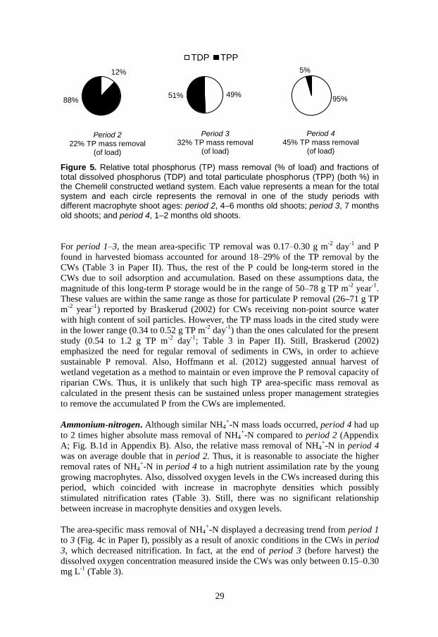
29

Figure 5. Relative total phosphorus (TP) mass removal (% of load) and fractions of total dissolved phosphorus (TDP) and total particulate phosphorus (TPP) (both %) in the Chemelil constructed wetland system. Each value represents a mean for the total system and each circle represents the removal in one of the study periods with different macrophyte shoot ages: period 2, 4–6 months old shoots; period 3, 7 months old shoots; and period 4, 1–2 months old shoots.

For period 1–3, the mean area-specific TP removal was 0.17–0.30 g m-2

day-1

and P

found in harvested biomass accounted for around 18–29% of the TP removal by the

CWs (Table 3 in Paper II). Thus, the rest of the P could be long-term stored in the

CWs due to soil adsorption and accumulation. Based on these assumptions data, the

magnitude of this long-term P storage would be in the range of 50–78 g TP m-2

year-1

.

These values are within the same range as those for particulate P removal (26–71 g TP

m-2

year-1

) reported by Braskerud (2002) for CWs receiving non-point source water

with high content of soil particles. However, the TP mass loads in the cited study were

in the lower range (0.34 to 0.52 g TP m-2

day-1

) than the ones calculated for the present

study (0.54 to 1.2 g TP m-2

day-1

; Table 3 in Paper II). Still, Braskerud (2002)

emphasized the need for regular removal of sediments in CWs, in order to achieve

sustainable P removal. Also, Hoffmann et al. (2012) suggested annual harvest of

wetland vegetation as a method to maintain or even improve the P removal capacity of

riparian CWs. Thus, it is unlikely that such high TP area-specific mass removal as

calculated in the present thesis can be sustained unless proper management strategies

to remove the accumulated P from the CWs are implemented.

Ammonium-nitrogen. Although similar NH4+-N mass loads occurred, period 4 had up

to 2 times higher absolute mass removal of NH4+-N compared to period 2 (Appendix

A; Fig. B.1d in Appendix B). Also, the relative mass removal of NH4+-N in period 4

was on average double that in period 2. Thus, it is reasonable to associate the higher

removal rates of NH4+-N in period 4 to a high nutrient assimilation rate by the young

growing macrophytes. Also, dissolved oxygen levels in the CWs increased during this

period, which coincided with increase in macrophyte densities which possibly

stimulated nitrification rates (Table 3). Still, there was no significant relationship

between increase in macrophyte densities and oxygen levels.

The area-specific mass removal of NH4+-N displayed a decreasing trend from period 1

to 3 (Fig. 4c in Paper I), possibly as a result of anoxic conditions in the CWs in period

3, which decreased nitrification. In fact, at the end of period 3 (before harvest) the

dissolved oxygen concentration measured inside the CWs was only between 0.15–0.30

mg L-1

(Table 3).

12%

88%

Period 2 22% TP mass removal

(of load)

49% 51%

Period 3 32% TP mass removal

(of load)

TDP TPP

95%

5%

Period 4 45% TP mass removal

(of load)

30

Okurut et al. (1999) reported decreased NH4+-N removal, in CWs dominated by C.

papyrus and another species, and linked the low rates to low residual oxygen concentrations (< 2 mg L-1) in the CWs. Evidence of anoxic conditions in the Chemelil CWs was supported by observations of white precipitate and smell of sulfides at the outlets of all CWs in periods 2 and 3. Since turnover rates in tropical areas are rapid (1 to 3 months intervals; Reddy et al. 1999; Kadlec 2005a), above-ground biomass and subsequent decomposition of the litter likely created anaerobic conditions at the end of period 3, when the macrophytes had been growing for more than 6 months. Also, a net release of NH4

+-N from fragmentation of macrophyte litter in period 3 could have decreased removal of NH4

+-N (Reddy and Patrick 1984; Howard-Williams 1985).

TSS. In period 4, both relative and absolute mass removal of TSS were generally half

of those observed during the periods 2–3, despite similar mass loads This result,

demonstrated that the absence of mature and dense vegetation in the CWs in period 4

was negative for TSS removal (Appendix A; Fig. B.1e in Appendix B). In the early part of period 1, macrophyte shoots were around 3 months old and the mean relative mass removal of TSS was only 46% (Appendix A). However, as the macrophytes shoots grew and became older (periods 2 and 3) the relative mass removal of TSS increased to around 80%. Yet, in period 4, when the shoots were only 1–2 months old, the TSS mass removal again decreased to only 40%. Not surprisingly, fractions of TPP followed a similar trend (Fig. 5). Possible explanations for the low TSS removal were that resuspension of sediment particles became significant when the vegetation cover in the CWs was small and that some organic remains from the harvest were prevalent in the sediment. Instead, resuspension became more insignificant as the vegetation cover increased with macrophyte age. These results suggest that frequent harvesting of emergent macrophytes in CWs could improve TDP and NH4

+-N removal, however, at expense of lower TSS removal. However, this type of assumption should be confirmed in actual studies.

Treatment effects on pollutant concentrations. With the final data set (i.e. using k =

1.4 to estimate ET and the addition of period 4), significantly higher outflow

concentrations of TDP and NH4+-N, respectively, with increasing mass load were

observed (R2 = 0.46; p < 0.001 for TDP and R

2 = 0.38; p < 0.001 for NH4

+-N; Fig.

B.2b, d in Appendix B), which is representative treatment behaviour for CWs (Kadlec

and Wallace 2009). However, for TPP significantly lower outflow concentrations were

observed with increasing mass load (p < 0.001; Fig. B.2c in Appendix B). Also, a

multiple linear regression, showed that season had a significant effect on outflow

concentrations of TP, TDP and TSS, with a decreasing trend from period 1–4 for the

two former, but increasing for the latter (Fig. B.2a, b, e in Appendix B). This type of

CW treatment behaviour was likely connected to the inability of the CWs to retain

particles especially in period 4, yet a higher capacity to assimilate TDP.

Phosphorus. Paper I reported that the Chemelil CW system significantly reduced

inflow concentrations of all water quality parameters (Fig. 3a–d in Paper I). Still,

reviewing these results within current effluent guideline values of 2 mg TP L-1

(World

Bank Group 2007; NEMA 2006) all TP outflow concentrations did not meet these

requirements (Appendix A). The P outflow concentration from a CW is a function of

both mass load and the inflow concentration (Kadlec and Wallace 2009).

31

At the present mass loads (200–440 g TP m-2

year-1

) and inflow concentrations (5–6

mg TP L-1

) that the Chemelil CWs received, the literature suggests that outflow

concentrations of below 3 mg TP L-1

would be hard to achieve (Kadlec and Wallace

2009). Nevertheless, comparing outflow concentration of TP and TDP in period 4 with

those from period 2 points to the significance of P uptake by young growing

macrophyte shoots for achieving low effluent concentration of P from tropical CWs

(Fig. B.2a, b in Appendix B). Katsenovich et al. (2009) noted higher outflow

concentrations of TDP from FWS CWs dominated by C. papyrus during the dry

season compared to the rainy. This was also observed in the present study when

comparing results from periods 2 and 3 (Fig. B.2b in Appendix B.2). Still, adding

results from period 4 highlighted that, despite the lack of precipitation in dry periods,

young growing emergent macrophytes could assist in reducing outflow P

concentrations. For the Chemelil CW, since the inflow TP comprised of 75% TDP, this

study demonstrated that young growing macrophyte could play a significant role for

the achievement of effluent standard requirements.

Ammonium-nitrogen. All outflow concentrations of NH4+-N were of concern from a

discharge point of view (Appendix A), as nearly all values were above effluent standards set by the Kenyan National Environment Management Authority of 0.5 mg NH4

+-N L-1 for effluent discharge into the environment (NEMA 2006). Similarly to P results, generally higher outflow concentrations of NH4

+-N in period 2 compared to period 4, indicated that harvests, and thus young growing macrophytes, were important

for maintaining proper outflow concentrations of this parameter in tropical CWs (Fig.

B.2d in Appendix B.2).

Total suspended solids. Omitting results from period 4, removal of TSS was close to

the rule of thumb proposed by Kadlec and Knight (1996) that about 75% of incoming

TSS is removed if inflow concentrations of TSS are above 20 mg L-1

(Appendix A).

Also, during periods 1–3 the effluent guideline value of 50 mg TSS L-1

set up by the

World Bank Group (2007) and the standard 30 mg TSS L-1

set by NEMA (2006) was

achieved (Appendix A). However, in period 4, when the macrophytes had recently

been harvested, most CWs had an effluent of TSS that was 80–103% above the

standard set by NEMA (2006). Thus, comparing results from period 1–3 with those

from period 4 suggested that mature and dense vegetation may prevent problems to

meet regulatory requirements. Thus, well established vegetation may decrease

resuspension of particles and contribute to increased sedimentation of incoming

particles (Braskerud 2001) and effective filtering of solids (Kadlec 1994b).

5.1.3 EFFECTS OF MACROPHYTES

Paper I reported that the Chemelil CWs dominated by C. papyrus had significantly higher area-specific mass removal of NH4

+-N compared to those with E. pyramidalis.

The high efficiency of C. papyrus for treatment of NH4+-N in wastewater has

previously been noted by Okurut et al. (1999) and Kyambadde et al. (2005). Possibly, C. papyrus, allowed higher nitrification by having high root surface areas and thus

more nitrifying bacteria (Kyambadde et al. 2004). In the present study, roots of both species extended into the lower water column which could influence the redox status of the water close to the sediments.

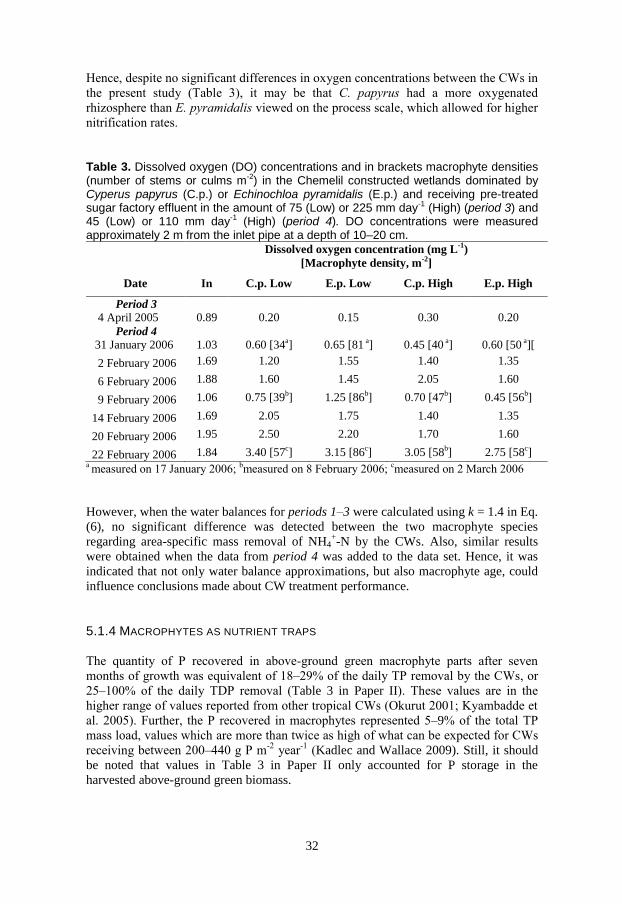
32

Hence, despite no significant differences in oxygen concentrations between the CWs in the present study (Table 3), it may be that C. papyrus had a more oxygenated rhizosphere than E. pyramidalis viewed on the process scale, which allowed for higher nitrification rates.

Table 3. Dissolved oxygen (DO) concentrations and in brackets macrophyte densities (number of stems or culms m-2) in the Chemelil constructed wetlands dominated by Cyperus papyrus (C.p.) or Echinochloa pyramidalis (E.p.) and receiving pre-treated sugar factory effluent in the amount of 75 (Low) or 225 mm day-1 (High) (period 3) and 45 (Low) or 110 mm day-1 (High) (period 4). DO concentrations were measured approximately 2 m from the inlet pipe at a depth of 10–20 cm.

Dissolved oxygen concentration (mg L-1

)

[Macrophyte density, m-2

]

Date In C.p. Low E.p. Low C.p. High E.p. High

Period 3

4 April 2005 0.89 0.20 0.15 0.30 0.20

Period 4

31 January 2006 1.03 0.60 [34a] 0.65 [81

a] 0.45 [40

a] 0.60 [50

a][

2 February 2006 1.69 1.20 1.55 1.40 1.35

6 February 2006 1.88 1.60 1.45 2.05 1.60

9 February 2006 1.06 0.75 [39b] 1.25 [86

b] 0.70 [47

b] 0.45 [56

b]

14 February 2006 1.69 2.05 1.75 1.40 1.35

20 February 2006 1.95 2.50 2.20 1.70 1.60

22 February 2006 1.84 3.40 [57c] 3.15 [86

c] 3.05 [58

b] 2.75 [58

c]

a measured on 17 January 2006; bmeasured on 8 February 2006; cmeasured on 2 March 2006

However, when the water balances for periods 1–3 were calculated using k = 1.4 in Eq.

(6), no significant difference was detected between the two macrophyte species

regarding area-specific mass removal of NH4+-N by the CWs. Also, similar results

were obtained when the data from period 4 was added to the data set. Hence, it was

indicated that not only water balance approximations, but also macrophyte age, could

influence conclusions made about CW treatment performance.

5.1.4 MACROPHYTES AS NUTRIENT TRAPS

The quantity of P recovered in above-ground green macrophyte parts after seven months of growth was equivalent of 18–29% of the daily TP removal by the CWs, or 25–100% of the daily TDP removal (Table 3 in Paper II). These values are in the higher range of values reported from other tropical CWs (Okurut 2001; Kyambadde et al. 2005). Further, the P recovered in macrophytes represented 5–9% of the total TP mass load, values which are more than twice as high of what can be expected for CWs receiving between 200–440 g P m-2 year-1 (Kadlec and Wallace 2009). Still, it should

be noted that values in Table 3 in Paper II only accounted for P storage in the

harvested above-ground green biomass.

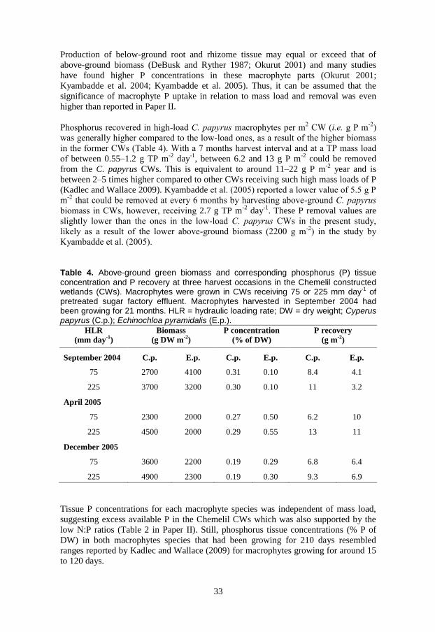
33

Production of below-ground root and rhizome tissue may equal or exceed that of

above-ground biomass (DeBusk and Ryther 1987; Okurut 2001) and many studies

have found higher P concentrations in these macrophyte parts (Okurut 2001;

Kyambadde et al. 2004; Kyambadde et al. 2005). Thus, it can be assumed that the

significance of macrophyte P uptake in relation to mass load and removal was even

higher than reported in Paper II.

Phosphorus recovered in high-load C. papyrus macrophytes per m2 CW (i.e. g P m-2) was generally higher compared to the low-load ones, as a result of the higher biomass in the former CWs (Table 4). With a 7 months harvest interval and at a TP mass load of between 0.55–1.2 g TP m

-2 day

-1, between 6.2 and 13 g P m

-2 could be removed

from the C. papyrus CWs. This is equivalent to around 11–22 g P m-2

year and is

between 2–5 times higher compared to other CWs receiving such high mass loads of P

(Kadlec and Wallace 2009). Kyambadde et al. (2005) reported a lower value of 5.5 g P m-2 that could be removed at every 6 months by harvesting above-ground C. papyrus biomass in CWs, however, receiving 2.7 g TP m

-2 day

-1. These P removal values are

slightly lower than the ones in the low-load C. papyrus CWs in the present study, likely as a result of the lower above-ground biomass (2200 g m-2) in the study by Kyambadde et al. (2005).

Table 4. Above-ground green biomass and corresponding phosphorus (P) tissue concentration and P recovery at three harvest occasions in the Chemelil constructed wetlands (CWs). Macrophytes were grown in CWs receiving 75 or 225 mm day-1 of pretreated sugar factory effluent. Macrophytes harvested in September 2004 had been growing for 21 months. HLR = hydraulic loading rate; DW = dry weight; Cyperus papyrus (C.p.); Echinochloa pyramidalis (E.p.).

HLR

(mm day-1

)

Biomass

(g DW m-2

)

P concentration

(% of DW)

P recovery

(g m-2

)

September 2004 C.p. E.p. C.p. E.p. C.p. E.p.

75 2700 4100 0.31 0.10 8.4 4.1

225 3700 3200 0.30 0.10 11 3.2

April 2005

75 2300 2000 0.27 0.50 6.2 10

225 4500 2000 0.29 0.55 13 11

December 2005

75 3600 2200 0.19 0.29 6.8 6.4

225 4900 2300 0.19 0.30 9.3 6.9

Tissue P concentrations for each macrophyte species was independent of mass load,

suggesting excess available P in the Chemelil CWs which was also supported by the

low N:P ratios (Table 2 in Paper II). Still, phosphorus tissue concentrations (% P of

DW) in both macrophytes species that had been growing for 210 days resembled

ranges reported by Kadlec and Wallace (2009) for macrophytes growing for around 15

to 120 days.

34

This result indicated a higher ability to sustain high P tissue concentrations for a longer

growing period, possibly due to the tropical conditions which stimulated year-round

nutrient uptake by the macrophytes. Also, these high tissue P concentrations in the

macrophyte biomass may possibly explain the higher significance of P removal via

harvesting compared to values found in Kadlec and Wallace (2009).

Nevertheless, the studied species seemed to have different growth strategies and P

uptake capacities. After 21 months of growth, harvested E. pyramidalis (September

2004) displayed significantly lower P tissue concentrations, and thus P recoveries, than

after the 7 months growth period (Table 4). Phosphorus tissue concentrations in C.

papyrus growing for 21 months were not markedly lower than from the shorter

growing periods. Also, biomass, and thus P recovery of C. papyrus, responded

positively to an increase in nutrient load which was not seen for E. pyramidalis (Table

4). These differences suggest that species-specific harvest strategies should be used,

where E. pyramidalis needs to be harvested more frequently than C. papyrus, in order

to maintain high area-specific P removal via macrophyte harvesting in the CWs.

Paper II and additional results presented in this thesis show that both biomass and

nutrient yields from macrophytes can be affected by harvest frequency, confirming

previous studies by Smith et al. (1991) and Koottatep and Polprasert (1997). The cited

studies indicate the possibility to harvest macrophytes for nutrients with much shorter

intervals than the 7 months intervals applied in Paper II. Okurut (2001) reported

maximum biomass (11 kg dwt m-2

) for C. papyrus after just 4 months of growth and

that the nutrient concentrations in tissues became stable at around 6 months growth.

This suggests that it is possible to maintain relatively high biomass (as g biomass m-2

CW), high P recovery (as g P m-2

CW) and good wastewater treatment results with

harvest intervals of less than 4 months. Moreover, harvesting with less than 4 months

intervals appears motivated, since turnover rates of above-ground biomass in tropical

areas are reported to occur at 1 to 3 months intervals (Reddy et al. 1999; Kadlec

2005a). Also, leaving part of CW intact at each harvest occasion might help in

preventing undesirable increases in outflows of TSS and associated TPP due to

resuspension of particles after the harvest. At the same time, as results in the present

thesis have suggested (Fig. 5), the harvested regions should stimulate nutrient

assimilation by young growing macrophytes and thus improve overall P and N

removal. Moreover, for high hydraulic efficiency, these unharvested vegetation

segments should be left as banded sections perpendicular to the inlet flow of the CW

(Jenkins and Greenway 2005). However, effects of these types of harvesting regimes

on water quality should be tested in actual studies.

5.2 THE HYDRAULIC TRACER STUDIES

Chemelil. The hydraulic tracer study described in Paper III was performed during period 4 in the Chemelil CWs in Kenya. The experiment was designed to study effects of macrophyte species and HLR, and also possible interaction effects of both factors on the hydraulic parameters e, N and (Eq. (1)–(3)). Also, simultaneously with the

tracer experiment samples for water quality were taken to investigate possible effects

of the hydraulic parameters on pollutant removal. The tracer data in Paper III was

analyzed using the method of moments (M).

35

Paper III reported no significant effect of either HLR (varied with a factor 2.4) or macrophyte species. Holland et al. (2004) and Wanko et al. (2010) both varied the inlet flow with a similar factor (1.9–2.4) as in Paper III (2.4) and found no effects of flow

on CW hydraulics. Macrophytes stems occupied between 0.2 and 3.8% of the CW

volume whereas water occupied 96.2–99.8% (Table 2 in Paper III). These relatively

low macrophyte volumes (compared to water volume) made detecting effects of

vegetation on CW hydraulics difficult. Thus, a condition with higher macrophyte

volumes and with more pronounced species characteristics could be a more proper

starting point to investigate effect of macrophyte species on CW hydraulics.

Analyzing the tracer data in Paper III using the gamma model revealed that outflow concentrations of NH4

+-N were significantly positively related to increasing e-values (p < 0.05; R2 = 0.58), i.e. that high outflow concentrations of NH4

+-N occurred at high effective volumes. Paper III reported decreasing e-values with increasing macrophyte densities in the CWs (Fig. 3 in Paper III). Hence, it was possible that low outflow concentrations of NH4

+-N were a result of higher macrophyte densities (i.e. lower e-values), pointing out that a dense macrophyte community is important for NH4

+-N removal in CWs (Kadlec and Wallace 2009). However, no significant relationship was found between outflow concentrations of NH4

+-N and macrophyte densities in the Chemelil CWs. Also, the gamma data analysis showed a significant decrease TDP outflow concentrations with increasing N-values (p < 0.05; R2 = 0.72) which confirm results by Dierberg et al. (2005), i.e. that there is a connection between hydraulic parameters and P removal in CWs. Also, the empirical results in the present thesis suggested that P removal in the CWs was more affected by the level of dispersion than of the amount of effective volume.

Halmstad. Paper IV describes the tracer study performed in the FWS CW system in Halmstad, Sweden in September–October 2008. The tracer experiment was designed to study effects of vegetation type (free development (FDW), emergent (EVW) or submerged (SVW)) and inlet design (barrier or no barrier), and their interaction effect on hydraulics. Tracer data was analyzed using the M and the Gauss model. Statistical

analysis with a two-way ANOVA revealed that there was a significant interaction

between barrier and vegetation on effective volume ratio (Table 3 in Paper IV). Further

separate one-way ANOVA analysis showed that EVWs without barrier had

significantly lower tracer mass recoveries compared to the others CWs with the same

inlet design (Paper IV), whereas no significant differences in tracer mass recoveries

were found for CWs with barrier. Thus, the lower tracer mass recoveries in the EVWs

without barrier were connected to an interaction between emergent vegetation and no

inlet barrier. These result demonstrated that the methodology of tracer studies

performed in CWs with dense emergent vegetation could be improved by promoting

distribution of point-incoming tracer solution using a narrow barrier near the inlet.

Hence, in Paper IV, only results from CWs with barrier were considered to represent

the best data for further discussions. Also, in the present thesis, tracer data in Paper IV

were analyzed with the gamma model, which revealed that CWs with barrier had

significantly lower N-values i.e. higher dispersion (p < 0.01). Thus, it is possible that

the barrier aided the mixing of tracer into the CWs. Moreover, a two-way ANOVA

analysis with the gamma data showed that tracer mass recoveries were significantly

higher from CWs with barrier compared to those without barrier (p < 0.05).

36

This new result supports the decision to use data from CWs with barrier in the

discussion in Paper IV. Nevertheless, results in Paper IV showed significantly lower e-

values from EVWs compared to SVWs and FDWs, and thus conferred that the lower

e-values in EVWs were related to dense living macrophyte and accumulated dead

macrophyte parts. Hence, both Paper III and IV support that emergent vegetation does

significantly affect the effective volume in CWs and highlights the need for regulating

dense emergent vegetation in CWs to secure efficient volume for treatment.

5.2.1 EFFECTS OF TRACER DATA ANALYSIS METHOD

In Paper IV significantly different hydraulic parameter values were obtained as a result

using different data analysis methods (Table 5 in Paper IV). Also, analyzing the tracer

data in Paper IV with the gamma model resulted in yet another set of e-and N-values

that were generally significantly different from those presented in Paper IV. The

gamma model consistently resulted in on average 45% lower e-values than those from

the other two methods used in Paper IV (Appendix D). The N-values produced by the

gamma model were on average 380% higher than those reported in Paper IV.

Moreover, using the gamma model to analyze the tracer data in Paper III revealed that

both e-and N-values were significantly different than those from the M (Appendix C).

The gamma model produced e-values that were on average 25% lower whereas the N-

values were on average 100% higher compared to the M. Thus, both analyzing data

from Paper III and IV with the gamma model showed that this model generally

produced lower e-values but higher N-values compared to others methods used in

Paper III and IV. Also, data from other studies confirm that that e-values from the M

are generally higher (5–48%) than those from the gamma model. Similarly, the N

values from the M may be 29–89% lower compared to those obtained from the gamma

model (Wang and Jawitz 2006; Kadlec and Wallace 2009). But what do these

discrepancies between data analysis methods mean for wastewater treatment results

from CWs?

Using data from Paper III, outflow concentrations (Cout) and e-values from the gamma

model and those obtained by the M, respectively, were calculated using the plug model

(Eq. (8)).

)(exp nxv tek

inout CC

(8)

where Cin is the inflow concentration (mg L-1

), exp is the natural logarithm; ex is the

effective volume ratio (obtained from either the gamma model or the method of

moments); kv is the volumetric reaction rate coefficient (day-1

) and tn is the theoretical

residence time of the CW (day). The kv-value in Eq. (8) was arbitrary set to 0.082 day-

1, the inflow concentration (Cin) to 5 mg L

-1 and the tn-value to 5 days.

The relative error of the two outflow concentrations (Eq. (8)) and also the relative error

of the effective volumes obtained by either the gamma model or the M, were

calculated separately using Eq. (9).

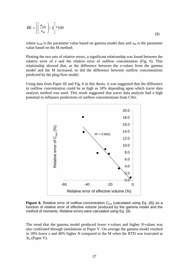
37

100*1

M

GM

x

xRE

(9)

where xGM is the parameter value based on gamma model data and xM is the parameter

value based on the M method.

Plotting the two sets of relative errors, a significant relationship was found between the

relative error of e and the relative error of outflow concentration (Fig. 6). This

relationship showed that, as the difference between the e-values from the gamma

model and the M increased, so did the difference between outflow concentrations

predicted by the plug-flow model.

Using data from Paper III and Fig. 6 in this thesis, it was suggested that the difference

in outflow concentration could be as high as 18% depending upon which tracer data

analysis method was used. This result suggested that tracer data analysis had a high

potential to influence predictions of outflow concentrations from CWs.

Figure 6. Relative error of outflow concentration Cout (calculated using Eq. (8)) as a function of relative error of effective volume produced by the gamma model and the method of moments. Relative errors were calculated using Eq. (9).

The trend that the gamma model produced lower e-values and higher N-values was

also confirmed through simulations in Paper V. On average the gamma model resulted

in 18% lower e and 40% higher N compared to the M when the RTD was truncated at

3tn (Paper V).

R² = 0.9061

0.0

2.0

4.0

6.0

8.0

10.0

12.0

14.0

16.0

18.0

20.0

-60 -40 -20 0

Re

lative

err

or

of C

out (%

)

Relative error of effective volume (%)

38

In Paper V, simulation results of e and N from the gamma model were also compared

to those obtained from the M when the RTD was truncated at tracer background

concentration. Truncating at background levels normally meant truncating before 3tn

(usually between 1.1 to 2.5tn). Results showed that e-values from the gamma model

were on average only 1% lower than those from the M truncated at tracer background

concentration. The corresponding values for N were 2% higher than those from the

gamma model. Thus, Paper V showed that differences between tracer data analysis

methods can be reduced if the M uses a suitable RTD truncation method, i.e. by

truncating at tracer background concentration. Thus, currently a cautionary principle is

justified when analysing tracer data from FWS CWs, where the use of two methods

and comparing their results could be advantageous as opposed to using only one

method. These types of comparisons could also possibly help future methodological

refinements and lead to more accurate hydraulic data and CW treatment results.

The literature review performed in Paper V revealed that the most common method for

RTD analysis was the M with RTD truncation at 3tn. Comparing parameter results

from the M with RTD truncation at 3tn with those from the gamma model and also the

M with tracer background concentrations, showed that the former method produced on

average 25% higher e- and 31% lower N-values (Paper V). Thus, both results from the

literature review and simulations in Paper V indicated that published articles may

contain overestimated e- and underestimated N-values. Consequently, pollutant

removal rates estimated by the TIS model may also be overestimated by as much as

13%, compared to using the M with RTD truncation at background levels or gamma

modelling (Paper V). Moreover, results in Paper V demonstrated that the frequent use

of the M with RTD truncations at 3tn or higher may result in unrealistic e-values

(higher than 100%). Formerly, e values higher than 100% have mainly been ascribed

to errors in water flow measurements or estimations of the theoretical CW volume

(Kadlec 1994a; Kjellin et al 2007) or simply viewed as unproblematic (Keefe et al.

2004; Dierberg et al. 2005; Kusin et al. 2012). However, results from this thesis

suggest that the occurrence of unrealistic e-values found in the literature could to some

degree be explained by the choice of tracer data analysis method. Therefore, to obtain

more reliable hydraulic data and treatment results from FWS CWs more attention

should be focused on tracer data analysis methods.

39

6. CONCLUSIONS

This thesis provides some answers as to how factors such as vegetation, hydraulics and

data analysis methods may affect results of wastewater treatment in free water surface

(FWS) constructed wetlands (CWs). Overall, results showed that meeting effluent

concentration standards simultaneously for all water quality parameters in one CW

was difficult. Low outflow concentrations of P and NH4+-N from the studied CWs

were observed when the macrophyte shoots were young (1–2 months). In contrast, the

TSS effluent standard was met when the macrophytes had been growing for at least 3–

4 months. This indicated that one possible way to connect the different requirements

for effective treatment of each substance is to leave banded vegetation sections

(perpendicular to the inflow direction) in the CWs intact at each harvest occasion. This

could reduce the risk of undesirable increased outflows of TSS, due to resuspension of

particles after the harvest, but at the same time, stimulate nutrient assimilation by

young growing macrophytes, and thus improve overall removal of P and N. Also,

especially, in tropical CWs, macrophyte harvesting during the dry season could be a

technique to keep both outflow concentrations of nutrients low and area-specific mass

removal high.

Paper I demonstrated that increases in mass load resulted in higher area-specific

removal, however, generally at the expense of higher outflow concentrations. Also, C.

papyrus dominated CWs had significantly higher area-specific mass removal of NH4+-

N compared to E. pyramidalis dominated ones. However, the significance of this effect

was dependent of how the evapotranspiration (ET) of the CWs was calculated, which

demonstrated that conclusions about treatment performance of tropical CWs were

strongly influenced by ET estimates.

Paper II demonstrated that the P uptake by emergent macrophytes could represent

nearly one-third the overall removal of total P by tropical CWs. Still, in order to

optimize nutrient removal through macrophytes and reach optimal wastewater

treatment, harvest should occur at least every 4 months and be species-specific.

Paper III and IV reported that mature and high densities of emergent vegetation may

lead to significantly reduced effective volumes (e-values) in CWs. Thus, these papers

pointed out the significance of regulating of dense emergent vegetation in CWs to

secure efficient volumes for wastewater treatment. Paper IV also showed that tracer

studies with lithium chloride performed in CWs with dense emergent vegetation could

display problems related to poor tracer recoveries, increasing uncertainties in obtained

hydraulic parameters. However, this problem could be diminished by promoting the

distribution of incoming tracer solution using a narrow barrier near the CW inlet.

Paper V demonstrated that the method of moments (M) with RTD truncation at 3 times

the hydraulic residence time (tn) on average resulted in higher e- (25%) and lower (-

31%) N-values compared to the M with RTD truncation at background concentration

or gamma modelling. Nevertheless, discrepancies between the two mentioned data

analysis methods could be minimized, by truncating the RTD at tracer background

concentrations when the M was used. Thus, at present a cautionary principle is

justified, where more than one type of tracer data analysis method is used. Also, these

types of comparisons could also possibly help future methodological refinements

within the field of tracer data analysis methods.

40

Paper V revealed that the most common method in the published literature in the last

25 years for tracer data analysis from FWS CWs was the M with RTD truncation at

3tn. This indicated that overestimated e- and underestimated N-values may be common

in published articles. As a result, pollutant removal rates by CWs may also be

overvalued by 13% compared to using other RDT truncation methods or modelling of

the tracer data. Also, Paper V demonstrated that the common use of the M with RTD

truncations at 3tn or above could result in unrealistic e-values (above 100%). Thus,

results in the present thesis indicated that occurrences of e-values above 100% found

in the literature could to some degree be explained by the choice of tracer data analysis

method. Therefore, to obtain more reliable hydraulic data and treatment results from

FWS CWs, more attention should be focused on the tracer data analysis methodology.

7. FUTURE STUDIES

To further improve and better control the wastewater treatment performance in

constructed wetlands (CWs), more controlled studies involving effects of important

factors such as vegetation and hydraulics are necessary. The knowledge surrounding

hydraulics and how it affects wastewater treatment in CWs is still very limited.

Specifically, there is still very little knowledge about effects of vegetation types or

species on CW hydraulics and possible connections to treatment. Thus, interesting

studies would be those involving simultaneous water quality monitoring and hydraulic

tracer studies in CWs with different vegetation types and/or species. Also, the effect on

wastewater treatment due to different macrophyte harvest techniques in both time and

space should be studied. Possible studies could involve harvesting CWs in banded

sections perpendicular to the inflow direction (thus leaving part of the CW

unharvested) and include tracer experiments and water quality monitoring in order to

investigate how the water flow and treatment performance changes over time as a

result of the specific harvest technique used. Preferably, these types of studies should

first be done in pilot-scale CWs and then followed up in full-scale ones. Moreover,

another area warranting further research is to empirically explore if hydraulic

parameter values derived from tracer studies are affected by the type of tracer used in

combination with a certain data analysis method. More specifically, the question raised

could be: is there an interaction between type of tracer and type of data analysis

method which significantly affects the hydraulic parameter values?

To better understand and predict the behaviour of wastewater treating CWs in tropical

regions, studies in pilot-scale CWs are vital. These types of studies need to focus on

collecting long-term water quality data under different types of conditions, i.e. dry and

wet season and/or different macrophyte harvest regimes. Interesting studies would be

to investigate effects of macrophytes harvests executed at different seasons (wet and

dry) on water quality.

Overall, long term monitoring water quality together with surveys of fauna and flora

species are needed are to gain more knowledge and to optimize the diverse functions

that wetlands offer. In developing countries, CWs could offer other values than “just”

wastewater treatment such as macrophyte biomass recoveries and possibly eco-tourism

attracted by interesting wildlife that inhabit the wetland areas.

41

8. ACKNOWLEDGEMENTS

The present doctoral thesis was funded by the Department for Research Cooperation

(SAREC) of the Swedish International Development Agency (Sida) through Karin

Tonderski, the Ångpanneföreningens Research Foundation, and the Wala and Folke

Danielsson fund.

I want to thank the Chemelil Sugar Company Ltd. for enthusiastic support during my

experiments at their constructed wetland site. I am above all indebted to the Agronomy

Laboratory and Mr J. Odenge, Mr B. Odhiambo Owour, and Mr B. C. Nyamosi, not

only for help with field measurements, sampling, and laboratory issues but also for

making my work in Kenya a pleasant experience. I also want to thank Dr P. O. Raburu

for being the local coordinator of the larger project that included the present doctoral

project. Also, I wish to thank Charlotte Billgren for valuable company and support

during our common stays in Kenya.

I want to particularly thank my supervisor Karin Tonderski for giving me the

opportunity to start as a PhD student and for valuable help during the first part of my

project time and for the continued financial support throughout the project.

Also, I want to thank my supervisor Jesper Persson for being supportive of my ideas,

yet, giving me valuable training related to critical scientific thinking. Also, I am

thankful for the patience that Jesper has shown over the years and the opportunities he

has given me to evolve within the field of wetland hydraulics. A special gratitude is

directed to my co-supervisor Stefan Weisner for giving me the confidence to conduct

the work related to Paper IV and for the assistance during the writing process and

discussions related to statistical data analysis. I am also very thankful towards Anna

Mietto who conducted the fieldwork related to the tracer experiment and Per Magnus

Ehde for the Li+ analyses related to Paper IV. Also, I wish to thank my co-supervisor

Per Milberg for invaluable help and support related to Paper V and for the finalization

of my PhD thesis.

I want to thank my mother Vera and my father Rade for caring for my dog Inuita

during my long stays in Kenya or Linköping. In addition, I am thankful for all the

baby-sitting that both my parents and in-laws Eva and Kenneth Bodin have done in the

last 5 years. Also, I wish to thank Magnus Bodin for several discussions related to

mathematical issues during the writing of this doctorate thesis and the papers therein.

Further acknowledgments may be found in each separate Paper.

When I started my PhD project I had no children, however, now I have two children.

Thank you Elin and Anton for being a source of daily happiness for me and always

“taking me down to earth” whenever I got too wrapped up in work.

42

REFERENCES

Abila, R. (1998) Utilisation and economic valuation of the Yala swamp wetland,

Kenya. In: Strategies for wise use of wetlands: best practices in participatory

Management. Proceedings of Workshop held at the 2nd

International

Conference on Wetlands and Development (Dakar, Senegal), Gawler, M. (ed.),

IUCN, The World Conservation Union/Wetlands International/World Wide

Fund of Nature, pp. 89–95.

Abira, M.A., Ngirigacha, H.W. & van Bruggen, J.J.A. (2003) Preliminary

investigation of the potential of four tropical emergent macrophytes for

treatment of pre-treated pulp and papermill wastewater in Kenya. Water Sci.

Technol. 48, 223–231.

Bastviken, K.S., Eriksson, P.G., Martins, I., Neto, J., Leonardsson, L. & Tonderski, K.

(2003) Potential nitrification and denitrification on different surfaces in a

constructed treatment wetland. J. Environ. Qual. 32, 2414–2420.

Beeton, A.M. (2002) Large freshwater lakes: present state, trends, and future. Environ.

Conser. 29, 21–38.

Blahnik, T. & Day, J.J. (2000) The effects of varied hydraulic and nutrient loading

rates on water quality and hydrologic distributions in a natural forested

treatment wetland. Wetlands 20, 48–61.

Boesch, D.F., Brinsfield, R.B. & Magnien, R.E. (2001) Chesapeake Bay

Eutrophication: Scientific Understanding, Ecosystem Restoration, and

Challenges for Agriculture J. Environ. Qual. 30, 303–320.

Bojcevska, H. (2007) Treatment wetlands in a tropical climate. Licentiate thesis.

Institute of Technology, Linköping University, Linköping.

Borin, M. & Salvato, M. (2012) Effects of five macrophytes on nitrogen remediation

and mass balance in wetland mesocosms. Ecol. Eng. 46, 34–42.

Boutilier, L., Jamieson, R., Gordon, R. & Lake, C. (2008) Transport of Lithium Tracer

and E. coli in Agricultural Wastewater Treatment Wetlands. Water Qual. Res.

J. Can. 43, 110–117.

Boutilier, L., Jamieson, R., Gordon, R. & Lake, C. (2011) Modeling E. coli fate and

transport in treatment wetlands using the water quality analysis and simulation

program. J. Environ. Sci. Heal. A 46, 680–691.

Braskerud, B.C. (2001) The influence of vegetation on sedimentation and resuspension

of soil particles in small constructed wetlands. J. Environ. Qual. 30, 1447–

1457.

Braskerud B.C. (2002) Factors affecting phosphorus retention in small constructed

wetlands treating agricultural non-point source pollution. Ecol. Eng. 19, 41–61.

Brisson, J. & Chazarenc, F. (2009) Maximizing pollutant removal in constructed

wetlands: Should we pay more attention to macrophyte species selection? Sci.

Total Environ. 407, 3923–3930.

Brix, H. (1997) Do macrophytes play a role in constructed treatment wetlands? Water

Sci. Technol. 35, 11–17.

Brix, H. (1999) How 'green' are aquaculture, constructed wetlands and conventional

wastewater treatment systems? Water Sci. Technol. 40, 45–50.

Brix, H., Koottatep, T., Fryd, O. & Laugesen, C.H. (2011) The flower and the butterfly

constructed wetland system at Koh Phi Phi–System design and lessons learned

during implementation and operation. Ecol. Eng. 37, 729–735

Carleton, J.N. & Montas, H.J. (2010) An analysis of performance models for free

water surface wetlands. Water Res. 44, 3595–3606.

43

da Motta Marques, D.M.L., Leite, G.R. & Giovannini, S.G.T. (2000) Performance of

two macrophyte species in experimental wetlands receiving variable loads of

anaerobically treated municipal wastewater. Water Sci. Technol. 44, 311–316.

Dal Cin, L. & Persson, J. (2000) The influence of vegetation on hydraulic performance

in a surface flow wetland. In: Reddy KR & Kadlec RH (eds.), 7th International

Conference on Wetland Systems for Water Pollution Control. pp. 539–546.

IWA, Lake Buena Vista, Florida.

Dal Cin, L. & Bendoricchio, G. (2002) Influence of vegetation on the hydraulic

behaviour of a reconstructed wetland. Ecohydrology & Hydrobiology 2, 283–

288.

DeBusk, T.A. & Ryther, J.H. (1987) Biomass production and yields of aquatic

macrophytes. In: Aquatic macrophytes for water treatment and resource

recovery (eds. Reddy, K. R. & Smith, W. H.), pp. 579–598. Magnolia

Publishing Inc, Orlando, Florida.

Díaz, F.J., Chow, A.T., O’Geen, A.T., Dahlgren, R.A. & Po-Keung Wong, P.-K.

(2009) Effect of constructed wetlands receiving agricultural return flows on

disinfection byproduct precursors. Water Res. 43, 2750–2760.

Diemont, S.A.W. (2006) Mosquito larvae density and pollutant removal in tropical

wetland treatment systems in Honduras. Environ. Int. 32: 332–341.

Dierberg, F.E. & DeBusk, T.A. (2005) An evaluation of two tracers in surface-flow

wetlands: Rhodamine-WT and Lithium. Wetlands 25, 8–25.

Dierberg, F.E., Juston, J.J., DeBusk, T.A., Pietro, K. & Gu, B. (2005) Relationship

between hydraulic efficiency and phosphorus removal in a submerged aquatic

vegetation-dominated treatement wetland. Ecol. Eng. 25, 9–23.

Dudgeon, D., Arthington, A.H., Gessner, M.O., Kawabata, Z.-I., Knowler, D.J.,

Leverque, C., Naiman, R.J., Prieur-Richard, A.-H., Soto, D., Stiassny, M.L.J. &

Sullivan, C.A. (2006). Freshwater biodiversity: importance, threats, status and

conservation challenges. Biol. Rev. 81, 163–182.

Elser, J.J., Bracken, M.E.S., Cleland, E.E., Gruner, D.S., Harpole, W.S., Hillebrand,

H., Ngai, J.T., Seabloom, E.W., Shurin, J.B. & Smith, J.E. (2007) Global

analysis of nitrogen and phosphorus limitation of primary producers in

freshwater, marine and terrestrial ecosystems. Ecol. Lett. 10, 1135–1142.

Elser, J.J. (2012) Phosphorus: a limiting nutrient for humanity? Curr. Opin. Biotech.

23, 833–838.

Entrekin, S., Evans-White, M., Johnson, B. & Hagenbuch, E. (2011) Rapid expansion

of natural gas development poses a threat to surface waters. Front. Ecol.

Environ. 9, 503–511.

Eriksson, P.G. & Weisner, S.E.B. (1996) Functional differences in epiphytic microbial

communities in nutrient-rich freshwater ecosystems: An assay of denitrifying

capacity. Freshwater Biol. 36, 555–562.

Eriksson, P.G. & Andersson, J.L. (1999) Potential nitrification and cation exchange on

litter of emergent, freshwater macrophytes. Freshwater Biol. 42, 479–486.

Erler, D.V., Tait, D., Eyre, B.D. & Bingham, M. (2011) Observations of nitrogen and

phosphorus biogeochemistry in a surface flow constructed wetland. Sci. Total

Environ. 409, 5359–5367.

European Environment Agency (1995) In Stanners, D. & Bourdeau P. (eds), Europe’s

Environment: The Dobris Assessment. European Environment Agency,

Copenhagen.

44

Falkowski, P., Scholes, R.J., Boyle, E., Canadell, J., Canfield, D., Elser, J., Gruber, N.,

Hibbard, K., Hogberg, P., Linder, S., Mackenzie, F.T., Moore III, B., Pedersen,

T., Rosenthal, Y., Seitzinger, S., Smetacek, V. & Steffen, W. (2000) The global

carbon cycle: a test of our knowledge of Earth as a system. Science 290, 291–

296.

Fogler, H.S. (2006) Elements of Chemical Reactor Engineering. 4th

edition. Pearson

Education Inc., NJ: Prentice-Hall.

Forbes, E.G.A., Foy, R.H., Mulholland, M.V. & Brettell, J.L. (2011) Performance of a

constructed wetland for treating farm-yard dirty water. Water Sci. Technol. 64,

22–28.

Gagnon, V., Chazarenc, F., Kõiv, M. & Brisson, J. (2012) Effect of plant species on

water quality at the outlet of a sludge treatment wetland. Water Res. 46, 5305–

5315.

Gale P.M., Reddy K.R. & Graetz D.A. (1994) Phosphorus retention by wetland soils

used for treated wastewater disposal. J. Environ. Qual. 23, 370–377.

García-Lledóa, A., Ruiz-Ruedaa, O., Vilar-Sanza, A., Salab, L. & Bañeras, L. (2011)

Nitrogen removal efficiencies in a free water surface constructed wetland in

relation to plant coverage. Ecol. Eng. 37, 678–684.

Gearheart, R.A. (1992) Use of constructed wetlands to treat domestic wastewater, city

of Arcata, California. Water Sci. Technol. 26, 1625–1637.

Gerbens-Leenes, W. & Hoekstra, A.Y. (2012) The water footprint of sweeteners and

bio-ethanol. Environ. Int. 40, 202–211.

Gichuki, J., Guebas, F.D., Mugo, J., Rabour, C., Triest, L. & Dehairs, F. (2001)

Species inventory and the local uses of the plants and fishes of the Lower

Sondu Miriu wetland of Lake Victoria, Kenya. Hydrobiologia 458, 99–106.

Glasgow, H.B. Jr. & Burkholder, J.M. (2000) Water quality trends and management

implications from a five-year study of a eutrophic estuary. Ecol. Appl. 10,

1024–1046.

Gottschall, N., Boutin, C., Crolla, A., Kinsley, C. & Champagne, P. (2007) The role of

plants in the removal of nutrients at a constructed wetland treating agricultural

(dairy) wastewater, Ontario, Canada. Ecol. Eng. 29, 154–163.

Goulden C.E. (2011) The need for capacity building for biomonitoring of lakes and

streams in Asia. Lakes & Reservoirs: Research and Management 16, 159–163.

Goulet, R.R., Pick, F.R. & Droste, R.L. (2001) Test of the first-order removal model

for metal retention in a young constructed wetland. Ecol. Eng. 17, 357–371.

Government Bill 1997/98:145 (1997) Swedish Environmental Quality Objectives – An

Environmental policy for a sustainable Sweden.

Government Bill 2000/01:130 (2000) The Swedish Environmental Objectives – Interim

Targets and Action Strategies.

Gray, J.L. & Sedlak, D.L. (2005) The fate of estrogenic hormones in an engineered

treatment wetland with dense macrophytes. Water Environ. Res. 77, 24–31.

Greenway, M. & Woolley, A. (1999) Constructed wetlands in Queensland:

Performance efficiency and nutrient bioaccumulation. Ecol. Eng. 12, 39–55.

Groffman, P.M., Tiedje, J.M., Robertson, G.P. & Christensen, S. (1988)

Denitrification at different temporal and geographical scales: proximal and

distal controls. In: Wilson, J. R. (ed.), Advances in Nitrogen Cycling in

Agricultural Ecosystems. CAB International, Wallingford, UK, pp. 174–192.

Hammer, D.A. & Knight, R.L. (1994) Designing constructed wetlands for nitrogen

removal. Water Sci. Technol. 29, 15–27.

45

Hansson, L.-A. & Wilhelm Granéli, W. (1984) Effects of winter harvest on water and

sediment chemistry in a stand of reed (Phragmites australis). Hydrobiologia

112, 131–136.

Headley, T.R. & Kadlec, R.H. (2007) Conducting hydraulic tracer studies of

constructed wetlands: a practical guide. Ecohydrology & Hydrobiology 7, 269–

282.

Hoffmann C.C., Heiberg L., Audet J., Schønfeldt B., Fuglsang A., Kronvang B.,

Ovesen N.B., Kjaergaard C., Hansen H.C.B. & Jensen H.S. (2012) Low

phosphorus release but high nitrogen removal in two restored riparian wetlands

inundated with agricultural drainage water. Ecol. Eng. 46, 75–87.

Holland, J.F., Martin, J.F., Granata, T., Bouchard, V., Quigley, M. & Brown, L. (2004)

Effects of wetland depth and flow rate on residence time distribution

characteristics. Ecol. Eng. 23, 189–203.

Hopkinson, C.S. Jr. & Vallino, J.J. (1995) The Relationships among Man's Activities

in Watersheds and Estuaries: am of runoff effects on patterns of erstuarine

community metabolism. Estuaries 18, 598–621.

Howard-Williams, C. (1985) Cycling and Retention of Nitrogen and Phosphorous in

Wetlands: A Theoretical and Applied Perspective. Freshwater Biol. 15, 391–

431.

Ippolito, J.A., Barbarick, K.A. & Redente, E.F. (2002) Combinations of water

treatment residuals and biosolids affect two range grasses. Commun. Soil Sci.

Plan. 33, 831–844.

Isosaari, P., Hermanowicz, S.W. & Rubin, Y. (2010) Sustainable Natural Systems for

treatment and disposal of food processing wastewater. Crit. Rev. Env. Sci. Tec.

40, 662–697.

Jenkins, G.A. & Greenway, M. (2005) Hydraulic efficiency of fringing versus banded

vegetation in constructed wetlands. Ecol. Eng. 25, 61–72.

Jing, S.-R., Lin, Y.-F., Wang, T.-W. & Lee, D.-Y. (2002) Microcosm wetlands for

wastewater treatment with different hydraulic loading rates and macrophytes. J.

Environ. Qual. 31, 690–696.

Juwarkar, A.S., Oke, B., Juwarkar, A. & Patnaik, S.M. (1995) Domestic wastewater

treatment through constructed wetland in India. Water Sci. Technol. 40, 291–

294.

Kadlec, R.H. (1984). Aging phenomena in wastewater wetlands. In: Ecological

Considerations in Wetlands Treatment of Municipal Wastewaters, Godfrey, P.

J., Kaynor, E. R., Pelczarski, S. and Benforado, J. (eds.). van Nostrand

Reinhold Company, New York. pp. 338–350.

Kadlec, R.H. (1994a) Detention and mixing in free water wetlands. Ecol. Eng. 3, 345–

380.

Kadlec, R.H. (1994b) Wetlands for water polishing: free water surface wetlands. In:

Global Wetlands: Old World and New. Mitsch, W. J. (ed), pp. 335–349.

Elsevier, Columbus, Ohio.

Kadlec, R.H. (2003) Pond and wetland treatment. Water Sci. Technol. 48, 1–8.

Kadlec, R.H. (2005a) Phosphorus removal in emergent free surface wetlands. J.

Environ. Sci. Heal. 40, 1293–1306.

Kadlec, R.H. (2005b) Nitrogen farming for pollution control. J. Environ. Sci. Heal. 40,

1307–1330.

Kadlec, R.H. (2006) Water temperature and evapotranspiration in surface flow

wetlands in hot and arid climate. Ecol. Eng. 26, 328–340.

Kadlec, R.H. (2009). Wastewater treatment at the Houghton Lake wetland: hydrology

and water quality. Ecol. Eng. 35, 1287–1311.

46

Kadlec, R.H. & Knight, R.L. (1996) Treatment wetlands. CRC Press Inc., Boca Raton,

Florida.

Kadlec, R.H. & Wallace, S.D. (2009) Treatment wetlands. 2nd

edition. CRC Press,

Boca Raton, Florida.

Kadlec, R.H., Cuvellier, C. & Stober, T. (2010). Performance of the Columbia,

Missouri, treatment wetland. Ecol. Eng. 36, 672–684.

Kantawanichkul, S. & Duangjaisak, W. (2011) Domestic wastewater treatment by a

constructed wetland system planted with rice. Water Sci. Technol. 64, 2376–

2380.

Kaseva M.E. (2004) Performance of a subsurface flow constructed wetland in

polishing pre-treated wastewater - a tropical case study. Water Res. 38, 681–

687.

Katsenovich, Y.P., Hummel-Batista, A., Ravinet, A.J. & Miller, J.F. (2009)

Performance evaluation of constructed wetlands in a tropical region. Ecol. Eng.

35, 1529–1537.

Keefe, S.H., Barber, L.B., Runkel, R.L., Ryan, J.N., McKnight, D.M. & Wass, R.

(2004) Conservative and reactive solute transport in constructed wetlands.

Water Resour. Res. 40, W012011–W0120112.

Keefe, S.H., Daniels (Thullen), J.S., Runkel, R.L. & Wass, R.D. (2010) Influence of

hummocks and emergent vegetation on hydraulic performance in a surface flow

wastewater treatment wetland. Water Resour. Res. 46, 1–13.

Kim, S.-Y. & Geary, P.M. (2001) The impact of biomass harvesting on phosphorus

uptake by wetland plants. Water Sci. Technol. 44, 61–67

Kingsford, R.T. & Thomas, R.F. (2004) Destruction of wetlands and waterbird

populations by dams and irrigation on the Murrumbidgee river in arid

Australia. Environ. Manage. 34, 383–396.

Kivaisi, A.M. (2001) The potential for constructed wetlands for wastewater treatment

and reuse in developing countries: a review. Ecol. Eng. 16, 545–560.

Kjellin, J., Wörman, A., Johansson, H. & Lindahl, A. (2007). Controlling factors for

water residence time and flow patterns in Ekeby treatment wetland, Sweden.

Adv. Water Resour. 30, 838–850.

Klomjek, P. & Nitisoravut, S. (2005). Constructed treatment wetland: a study of eight

plant species under saline conditions. Chemosphere 58, 585–593.

Knight, R.L., Ruble R.W., Kadlec, R.H. & Reed, S. (1993). Wetlands for Wastewater

Treatment: Performance Database. In: Constructed wetlands for water quality

improvement, Moshiri, G.A. (eds.). CRC Press Inc, Boca Raton, Florida. pp.

35–58.

Ko, J.-Y., Day, J. W., Lane, R.L., Hunter, R., Sabins, D., Pintado, K.L. & Franklin, J.

(2012) Policy adoption of ecosystem services for a sustainable community: A

case study of wetland assimilation using natural wetlands in Breaux Bridge,

Louisiana. Ecol. Eng. 38, 114–118.

Koottatep, T. & Polprasert, C. (1997) Role of plant uptake on nitrogen removal in

constructed wetlands located in the tropics. Water Sci. Technol. 36, 1-8.

Krogstad, T., Sogn, T.A., Asdal, Å. & Sæbø, A. (2005) Influence of chemically and

biologically stabilized sewage sludge on plant-available phosphorous in soil.

Ecol. Eng. 25, 51–60

Kusin, F.M., Jarvis, A.P. & Gandy, C.J. (2010) Hydraulic residence time and iron

removal in a wetland receiving ferruginous mine water over a 4 year period.

Water Sci. Technol. 62, 1937–1194.

Kusin, F.M., Jarvis, A.P. & Gandy, C.J. (2012) Hydraulic performance assessment of

passive coal mine water treatment systems in the UK. Ecol. Eng. 49, 233-243.

47

Kutija, V. & Hong, H. (1996) A numerical model for assessing the additional

resistance to flow introduced by flexible vegetation. J. Hydraul. Res. 34, 99–

114.

Kyambadde, J., Kansiime, F., Gumaelius, L. & Dalhammar, G. (2004) A comparative

study of Cyperus papyrus and Miscanthidium violaceum-based constructed

wetlands for wastewater treatment in a tropical country. Water Res. 38, 475–

485.

Kyambadde, J., Kansiime, F. & Dalhammar, G. (2005). Nitrogen and phosphorus

removal in substrate-free pilot constructed wetlands with horizontal surface

flow in Uganda. Water, Air, and Soil Poll. 165, 37–59.

Lange J., Schuetz T., Gregoire C., Elsässer D., Schulz R., Passeport E. & Tournebize J.

(2011) Multi-tracer experiments to characterise contaminant mitigation

capacities for different types of artificial wetlands. Intern. J. Environ. Anal.

Chem. 91, 768–785.

Li, L., Li, Y., Biswas, D.K., Nian, Y. & Jiang, G. (2008) Potential of constructed

wetlands in treating the eutrophic water: Evidence from Taihu Lake of China.

Bioresource Technol. 99, 1656–1663.

Lightbody, A.F., Nepf, H.M. & Bays, J.S. (2007) Mixing in deep zones within

constructed treatment wetlands. Ecol. Eng. 29, 209–220.

Lim, P.E., Wong, T.F. & Lim, D.V. (2001) Oxygen demand, nitrogen and copper

removal by free-water surface and subsurface-flow constructed wetlands under

tropical conditions. Environ. Int. 26, 425-431.

Lindstrom, S.M. & White, J.R. (2011) Reducing phosphorus flux from organic soils in

surface flow treatment wetlands. Chemosphere 85, 625–629.

Lin, Y.-F., Jing, S.-R., Lee, D.-Y. & Wang, T.-W. (2002) Nutrient removal from

aquaculture wastewater using a constructed wetlands system. Aquaculture 209,

169–184.

Lung’ayia, H., Sitoki, L. & Kenyanya, M. (2001) The nutrient enrichment of Lake

Victoria (Kenyan waters). Hydrobiologia 458, 75–82.

Lü G., He H., Yang D., Cai X. & Jing Y. (2012) Cutting effects on growth and

wastewater purification of Cyperus alternifolius in constructed wetland.

Shengtai Xuebao/ Acta Ecologica Sinica, 32, 4932–4939.

Martin, J.F. & Reddy, K.R. (1997) Interaction and spatial distribution of wetland

nitrogen processes. Ecol. Model. 105, 1–21.

Martin, C.D., Johnson, K.D. & Moshiri, G.A. (1999) Performance of a constructed

wetland leachate treatment system at the Chunchula landfill, Mobile County,

Alabama. Water Sci. Technol. 40, 67–74.

Martín, M., Oliver, N., Hernández-Crespo, C., Gargallo, S. & Regidor, M.C. (2013)

The use of free water surface constructed wetland to treat the eutrophicated

waters of lake L'Albufera de Valencia (Spain). Ecol. Eng. 50, 52–61.

Martinez, C.J. & Wise, W.R. (2003) Hydraulic Analysis of Orlando Easterly Wetland.

J. Environ. Eng.-ASCE. 129, 553–560.

Matson, P.A., Parton, W.J., Power, A.G. & Swift, M.J. (1997) Agricultural

intensification and ecosystem properties. Science 277, 504–509.

Mashauri, D.A., Mulungu, D.M.M. & Abdulhussein, B.S. (2000) Constructed wetland

at the University of Dar es Salaam. Water Res. 34, 1135–1144.

Meutia, A.A. (2001) Treatment of laboratory wastewater in a tropical constructed

wetland comparing surface and subsurface flow. Water Sci. Technol. 44, 499–

506.

48

Min, J.-H. & Wise, W.R. (2009) Simulating short-circuiting flow in a constructed

wetland: The implications of bathymetry and vegetation effects. Hydrol.

Process. 23, 830–841.

Mitsch, W.J., Zhang, L., Christopher J. Anderson, C.J., Altor, A.E. & Hernández, M.E.

(2005) Creating riverine wetlands: ecological succession, nutrient retention,

and pulsing effects. Ecol. Eng. 25, 510–527.

Mitsch, W.J. & Gosselink, J.G. (2000) Wetlands. 3rd

edition. John Wiley and Sons,

New York.

Muyodi, F.J., Bugenyi, F.W.B. & Hecky, R.E. (2010) Experiences and lessons learned

from interventions in the Lake Victoria Basin: The Lake Victoria

Environmental Management Project. Lakes & Reservoirs: Research and

Management 15, 77–88.

NEMA (National Environment Management Authority). (2006) Environmental

management and co-ordination (water quality) regulations, 2006. Arrangement

of regulations. Kenya gazette supplement No. 68, Legal notice No.120.

(<http://www.nema.go.ke/index.php?option=com_content&view=article&id=1

36&Itemid=489> (accessed February 6, 2013).

Nepf, H.M. (1999) Drag, turbulence, and diffusion in flow through emergent

vegetation. Water Resour. Res. 35, 479–489.

Newman, J.M. & Clausen, J.C. (1997) Seasonal effectiveness of a constructed wetland

for processing milkhouse wastewater. Wetlands 17, 375–382.

Nichols, D.S. (1983). Capacity of natural wetlands to remove nutrients. J. Water

Pollut. Control Fed. 55, 495–503.

Okurut, T.O., Rijs, G.B.J., & van Bruggen, J.J.A. (1999) Design and performance of

experimental constructed wetlands in Uganda, planted with Cyperus papyrus

and Phragmites mauritianus. Water Sci. Technol. 40, 265–271.

Okurut, T.O. (2001) Plant growth and nutrient uptake in a tropical constructed

wetland. In: Transformations of nutrients in natural and constructed wetlands,

Vymazal, J. (eds.). Backhuys Publishers, Leiden, Netherlands. pp. 451–462.

Peacock, C.E. & Hess, T.M. (2004) Estimating evapotranspiration from a reed bed

using the Bowen ratio energy balance method. Hydrol. Process. 18, 247–260.

Perfler, R., Laber, J., Langergraber, G. & Haberl, R. (1999) Constructed wetlands for

rehabilitation and reuse of surface waters in tropical and subtropical areas - first

results from small-scale plots using vertical flow beds. Water Sci. Technol. 40,

155–162.

Persson, J. (2000) The Hydraulic Performance of Ponds of Various Layouts. Urban

Water 2, 243–250.

Persson J. (2005) The use of design elements in wetlands. Nord. Hydrol. 36, 113–120.

Persson, J., Somes, N.L.G. & Wong, T.H.F. (1999) Hydraulic efficiency of constructed

wetlands and ponds. Water Sci. Technol. 40, 291–300.

Persson J. & Wittgren H.B. (2003) How hydrological and hydraulic conditions affect

performance of ponds. Ecol. Eng. 21, 259–269.

Postel, S.L. & Carpenter, S.R. (1997) Freshwater ecosystem services. In: Nature's

services, Daily, G. E. (eds.). Island Press, Washington, DC, USA. pp. 195–214.

Richardson, C.J. (1985) Mechanisms Controlling Phosphorus Retention Capacity in

Freshwater Wetlands. Science 228, 1424–1426.

Richardson, C.J. & Marshall, P.E. (1986) Processes controlling movement, storage,

and export of phosphorus in a fen peatland. Ecol. Monogr. 56, 279–302.

Reddy, K.R. & Patrick, W.H. (1984) Nitrogen transformations and loss in flooded soils

and sediments. Crit. Rev. Env. Contr. 13, 273–309.

49

Reddy, K.R., Patrick, W.H. & Lindau, C.W. (1989) Nitrification-denitrification at the

plant root-sediment interface in wetlands. Limnol. Oceanogr. 34, 1004-1013.

Reddy K.R. & D´Angelo E.M. (1994) Soil processes regulating water quality in

wetlands. In: Global Wetlands: Old World and New (ed. Mitsch W.J.), pp. 309-

324. Elsevier, Columbus, Ohio.

Reddy, K.R., Kadlec, R.H., Flaig, E. & Gale, P.M. (1999) Phosphorus retention in

streams and wetlands: a review. Crit. Rev. Env. Sci. Tec. 29, 83–146.

Rodriguez, R. & Lougheed, V.L. (2010) The potential to improve water quality in the

middle Rio Grande through effective wetland restoration. Water Sci. Technol.

62, 501–509.

Ronkanen, A.-K. & Kløve, B. (2007) Use of stable isotopes and tracers to detect

preferential flow patterns in a peatland treating municipal wastewater. J.

Hydrol. 347, 418–429.

Rossmann, M., Teixeira de Matos, A., Carneiro Abreu, E., Fonseca e Silva, F. &

Carraro Borges, A. (2012) Performance of constructed wetlands in the

treatment of aerated coffee processing wastewater: Removal of nutrients and

phenolic compounds. Ecol. Eng. 49, 264–269.

Schmid, B.H., Hengl, M.A. & Stephan, U. (2004) Salt tracer experiments in

constructed wetland ponds with emergent vegetation: laboratory study on the

formation of density layers and its influence on breakthrough curve analysis.

Water Res. 38, 2095–2102.

Scholz, M., Harrington, R., Carroll, P. & Mustafa, A. (2010). Monitoring of nutrient

removal within integrated constructed wetlands (ICW). Desalination 250, 356–

360.

Smith, J., Seaton, J., Osuji, P., D´Aguiar, P., Chesney, P., McBean, M., Haynes, A.,

Harding, C. & Cumberbatch, N. (1991) Dry matter and crude protein yields of

Echinochloa pyramidalis on coastal clay soil of Guyana. Turrialba 41, 69–75

Smith, V.H. (2003) Eutrophication of freshwater and coastal marine ecosystems: A

global problem. Environ. Sci. Pollut. Res. 10, 126–139.

Sophocleous, M. (2004) Global and regional water availability and demand: prospects

for the future. Natural Resources Research 13, 61–75.

Sorrell, B.K. & Armstrong, W. (1994) On the difficulties of measuring oxygen release

by root systems of wetland plants. J. Ecol. 82, 177–183.

Soto-Jimenez, M.F., Paez-Osuna, F. & Bojorquez-Leyva, H. (2003) Nutrient cycling at

the sediment–water interface and in sediments at Chiricahueto marsh: a

subtropical ecosystem associated with agricultural land uses. Water Res. 37,

719–728.

Speer, S., Champagne, P., Crolla, A. & Kinsley, C. (2009) Hydraulic performance of a

mature wetland treating milkhouse wastewater and agricultural runoff. Water

Sci. Technol. 59, 2455–2462.

Stowell, R., Ludwig, R., Colt., J. & Tchobanoglous, G. (1981) Concepts in Aquatic

Treatment System Design. J. Environ. Eng. Div. ASCE. 107(EE5), 919–940.

Strand, J.A. & Weisner, S.E.B. (2013) Effects of wetland construction on nitrogen

transport and species richness in the agricultural landscape-Experiences from

Sweden (Article in press). Ecol. Eng.

Thackston E.L., Shields F.D.J. & Schroeder P.R. (1987) Residence time distributions

of shallow basins. J. Environ. Eng-ASCE 113, 1319–1332

Thullen, J.S., Sartoris, J.J. & Nelson, S. M. (2005) Managing vegetation in surface-

flow wastewater-treatment wetlands for optimal treatment performance. Ecol.

Eng. 25, 583–593.

50

Toet, S., Bouwman, M., Cevaal, A. & Verhoeven, J.T.A. (2005) Nutrient Removal

Through Autumn Harvest of Phragmites australis and Thypha latifolia Shoots

in Relation to Nutrient Loading in a Wetland System Used for Polishing

Sewage Treatment Plant Effluent. J. Environ. Sci. Heal. A. 40, 1133–1156.

Towler, B.W., Cahoon, J.E. & Stein, O.R. (2004) Evaporation crop coefficients for

cattail and bulrush. J. Hydrol. Eng. 9, 235–239.

Trepel, M. & Palmeri, L. (2002) Quantifying nitrogen retention in surface flow

wetlands for environmental planning at the landscape-scale. Ecol. Eng. 19,

127–140.

Vymazal, J. (2001) Transformations of nutrients in natural and constructed wetlands.

Backhuys Publishers, Leiden.

Vymazal, J. (2007) Removal of nutrients in various types of constructed wetlands. Sci.

Total Environ. 380, 48–65.

Vymazal, J. (2011) Constructed wetlands for wastewater treatment: five decades of

experience. Environ. Sci. Technol. 45, 61–69.

Wallace, S.D. & Knight, R.L. (2006). Small-scale constructed wetland treatment

systems: feasibility, design criteria, and O & M requirements. Final Report,

Project 01-CTS-56. Water Environment Research Foundation (WERF),

Alexandria, Virginia.

Walsh, J. (1991a) The greening of the Green Revolution. Science, New Series 252, 26.

Walsh, J.J. (1991b) Importance of continental margins in the marine biogeochemical

cycling of carbon and nitrogen. Nature 350, 53–55.

Wang, H. & Jawitz, J.W. (2006) Hydraulic analysis of cell-network treatment

wetlands. J. Hydrol. 330, 721–734.

Wang, H., Jawitz, J.W., White, J.R., Martinez, C.J. & Sees, M.D. (2006) Rejuvenating

the largest municipal treatment wetland in Florida. Ecol. Eng. 26, 132–146.

Wanko, A., Zhang, J.B., Mosé, R., Gregoire, C. & Sadowski, A. (2010) Hydraulic

parameters and statistical residence time distribution moments correlations - a

lysimeter study for pesticides mitigation. Int. J. Environ. An. Ch. 90, 299–310.

Wetzel, R.G. (2001) Limnology: Lake and River Ecosystems. Third Ed. Academic

Press, San Diego, CA.

Wittgren, H.B. & Mæhlum, T. (1997) Wastewater treatment wetlands in cold

climates. Water Sci. Technol. 35, 45–53.

World Bank Group. (2007) Environmental, Health and Safety (EHS) Guidelines for

Sugar Manufacturing. International Finance Corporation.

World Bank. (2010) Sustaining water for all in a changing climate. World Bank Group

Implementation Progress Report of the Water Resources Sector Strategy. The

International Bank for Reconstruction and Development / The World Bank.

Report no. 57125. Washington, DC.

Wörman, A. & Kronnäs, V. (2005) Effect of pond shape and vegetation heterogeneity

on flow and treatment performance of constructed wetlands. J. Hydrol. 301,

123–138.

Yang, Q., Chen, Z.-H., Zhao, J.-G. & Gu, B.-H. (2007) Contaminant Removal of

Domestic Wastewater by Constructed Wetlands: Effects of Plant Species. J.

Integr. Plant Biol. 4, 437–446.

APPENDICES

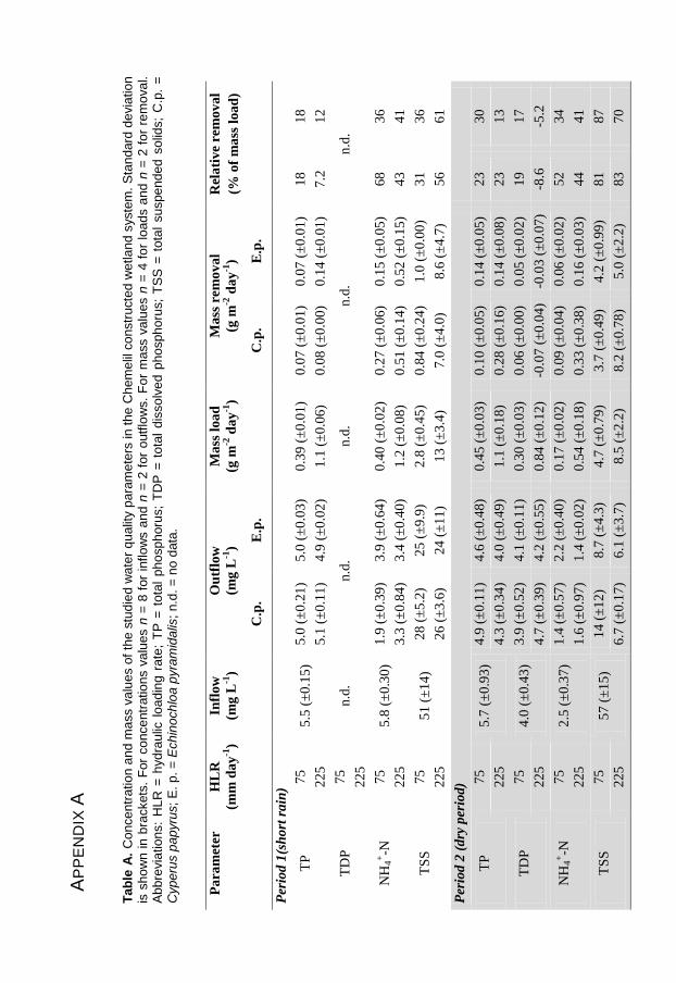
Tab

le A

. C

oncentr

ation a

nd m

ass v

alu

es o

f th

e s

tudie

d w

ate

r q

ualit

y p

ara

mete

rs in t

he C

hem

elil

constr

ucte

d w

etland s

yste

m.

Sta

ndard

devia

tion

is s

how

n in b

rackets

. F

or

concentr

ations v

alu

es n

= 8

for

inflow

s a

nd n

= 2

for

outf

low

s.

For

mass v

alu

es n

= 4

for

loads a

nd

n =

2 f

or

rem

oval.

Abbre

via

tions:

HLR

= h

ydra

ulic

loadin

g r

ate

; T

P =

tota

l phosphoru

s;

TD

P =

tota

l dis

solv

ed p

hosphoru

s;

TS

S =

to

tal

suspended s

olid

s;

C.p

. =

C

yperu

s p

apyru

s;

E. p. =

Echin

ochlo

a p

yra

mid

alis

; n.d

. =

no d

ata

.

Pa

ram

eter

HL

R

(mm

day

-1)

Infl

ow

(mg L

-1)

Ou

tflo

w

(mg L

-1)

Mass

load

(g m

-2 d

ay

-1)

Mass

rem

oval

(g m

-2 d

ay

-1)

(g m

-2 d

ay

-1)

Rel

ati

ve

rem

oval

(% o

f m

ass

load

)

C.p

. E

.p.

C.p

. E

.p.

Per

iod 1

(sh

ort

ra

in)

TP

7

5

5.5

(±

0.1

5)

5.0

(±

0.2

1)

5.0

(±

0.0

3)

0.3

9 (

±0.0

1)

0.0

7 (

±0.0

1)

0.0

7 (

±0

.01)

18

18

225

5.1

(±

0.1

1)

4.9

(±

0.0

2)

1.1

(±

0.0

6)

0.0

8 (

±0.0

0)

0.1

4 (

±0

.01)

7.2

12

TD

P

75

n.d

. n.d

. n.d

. n.d

. n.d

. 2

25

NH

4+-N

7

5

5.8

(±

0.3

0)

1.9

(±

0.3

9)

3.9

(±

0.6

4)

0.4

0 (

±0.0

2)

0.2

7 (

±0.0

6)

0.1

5 (

±0

.05)

68

36

225

3.3

(±

0.8

4)

3.4

(±

0.4

0)

1.2

(±

0.0

8)

0.5

1 (

±0.1

4)

0.5

2 (

±0

.15)

43

41

TS

S

75

51

(±

14

) 2

8 (

±5.2

) 25 (

±9.9

) 2.8

(±

0.4

5)

0.8

4 (

±0.2

4)

1.0

(±

0.0

0)

31

36

225

2

6 (

±3.6

) 24 (

±11)

13 (

±3.4

) 7.0

(±

4.0

) 8.6

(±

4.7

) 56

61

Per

iod 2

(d

ry p

erio

d)

TP

7

5

5.7

(±

0.9

3)

4.9

(±

0.1

1)

4.6

(±

0.4

8)

0.4

5 (

±0.0

3)

0.1

0 (

±0.0

5)

0.1

4 (

±0

.05)

23

30

225

4.3

(±

0.3

4)

4.0

(±

0.4

9)

1.1

(±

0.1

8)

0.2

8 (

±0.1

6)

0.1

4 (

±0

.08)

23

13

TD

P

75

4.0

(±

0.4

3)

3.9

(±

0.5

2)

4.1

(±

0.1

1)

0.3

0 (

±0.0

3)

0.0

6 (

±0.0

0)

0.0

5 (

±0

.02)

19

17

225

4.7

(±

0.3

9)

4.2

(±

0.5

5)

0.8

4 (

±0.1

2)

-0.0

7 (

±0.0

4)

-0.0

3 (

±0

.07)

-8.6

-5

.2

NH

4+-N

7

5

2.5

(±

0.3

7)

1.4

(±

0.5

7)

2.2

(±

0.4

0)

0.1

7 (

±0.0

2)

0.0

9 (

±0.0

4)

0.0

6 (

±0

.02)

52

34

225

1.6

(±

0.9

7)

1.4

(±

0.0

2)

0.5

4 (

±0.1

8)

0.3

3 (

±0.3

8)

0.1

6 (

±0

.03)

44

41

TS

S

75

57

(±

15

) 1

4 (

±12)

8.7

(±

4.3

) 4.7

(±

0.7

9)

3.7

(±

0.4

9)

4.2

(±

0.9

9)

81

87

225

6.7

(±

0.1

7)

6.1

(±

3.7

) 8.5

(±

2.2

) 8.2

(±

0.7

8)

5.0

(±

2.2

) 83

70

AP

PE

ND

IX A

Pa

ram

eter

HL

R

(mm

day

-1)

(mm

day

-1)

Infl

ow

(mg

L-1

)

Ou

tflo

w

(mg L

-1)

Mass

load

(g m

-2 d

ay

-1)

Mass

rem

oval

(g m

-2 d

ay

-1)

Rel

ati

ve

rem

oval

(% o

f m

ass

load

)

C

.p.

E.p

.

C.p

. E

.p.

Per

iod 3

(lo

ng

rain

)

TP

7

5

5.9

(±

0.5

7)

4.1

(±

0.0

9)

3.8

(±

0.2

8)

0.8

4 (

±0.1

9)

0.3

2 (

±0.0

8)

0.3

0 (

±0

.03)

37

39

225

4.3

(±

0.0

3)

3.7

(±

0.5

1)

1.2

2 (

±0.1

7)

0.2

5 (

±0.0

5)

0.3

9 (

±0

.02)

23

30

TD

P

75

4.9

(±

0.7

1)

3.8

(±

0.0

4)

3.8

(±

0.3

0)

0.6

9 (

±0.1

9)

0.2

1 (

±0.0

8)

0.2

1 (

±0

.04)

29

31

225

4.1

(±

0.0

3)

3.6

(±

0.4

7)

0.9

6 (

±0.1

7)

0.0

9 (

±0.0

3)

0.1

2 (

±0

.09)

10

11

NH

4+-N

7

5

4.6

(±

0.1

1)

4.5

(±

0.0

1)

4.8

(±

0.2

0)

0.6

1 (

±0.1

7)

0.0

4 (

±0.0

5)

0.0

0 (

±0

.02)

5.9

-0

.7

225

4.1

(±

0.4

6)

4.3

(±

0.1

6)

1.1

(±

0.1

2)

0.2

0 (

±0.1

0)

0.0

6 (

±0

.02)

19

5.5

TS

S

75

38

(±

5.4

) 12

(±

1.5

) 3.9

(±

1.3

) 5.5

(±

0.9

5)

4.3

(±

0.3

0)

4.1

(±

1.0

) 70

86

225

9

.7 (

±1.5

) 3.6

(±

1.8

) 8.6

(±

1.8

) 4.8

(±

0.3

2)

8.5

(±

0.1

9)

68

84

Per

iod 4

(d

ry p

erio

d)

TP

4

5

5.1

(±

0.2

4)

2.7

(±

0.0

6)

2.6

(±

0.1

7)

0.2

1 (

±0.0

0)

0.1

2 (

±0.0

1)

0.1

2 (

±0

.00)

56

58

110

3.5

(±

0.5

3)

3.6

(±

0.2

7)

0.5

1 (

±0.0

3)

0.1

7 (

±0.0

6)

0.1

5 (

±0

.01)

33

30

TD

P

45

4.0

(±

0.2

4)

1.7

1 (

±0.2

6)

1.1

2 (

±0.1

1)

0.1

6 (

±0.0

1)

0.1

0 (

±0.0

2)

0.1

3 (

±0

.02)

63

77

110

2.4

(±

0.1

1)

2.6

(±

0.0

3)

0.3

9 (

±0.0

4)

0.1

6 (

±0.0

0)

0.1

4 (

±0

.04)

40

35

NH

4+-N

4

5

3.5

(±

0.2

4)

1.3

(±

1.2

) 0.4

4 (

±0.2

8)

0.1

5 (

±0.0

2)

0.1

1 (

±0.0

2)

0.1

3 (

±0

.04)

70

87

110

0.9

1 (

±0.3

2)

1.1

(±

0.3

4)

0.3

4 (

±0.0

1)

0.2

5 (

±0.0

4)

0.2

4 (

±0

.05)

73

73

TS

S

45

85

(±

6.9

) 5

8(±

14)

61 (

±1.1

) 3.6

(±

0.2

8)

1.6

(±

0.6

3)

1.5

(±

0.2

2)

46

41

110

54

(±

5.0

) 60 (

±17)

8.7

(±

0.4

1)

3.5

(±

0.7

6)

2.0

(±

1.8

) 39

24

CO

NT. A

PP

EN

DIX

A

2

Figu

re B

.1. L

inea

r re

gres

sion

bet

wee

n m

ass

rem

oval

and

load

(bo

th g

m-2 d

ay-1)

for

(a)

TP, (

b) T

DP,

(c)

TPP

, (d)

NH

4+ -N a

nd (

e) T

SS in

the

Che

mel

il co

nstru

cted

wet

land

sys

tem

. Eac

h va

lue

repr

esen

ts o

ne w

etla

nd c

ell a

nd th

e m

ean

from

one

of f

our s

tudy

per

iods

. Abb

revi

atio

ns: T

P =

tota

l ph

osph

orus

; TD

P =

tota

l di

ssol

ved

phos

phor

us;

TPP

= to

tal

parti

cula

te

phos

phor

us;

TSS

= to

tal

susp

ende

d so

lids.

R² =

0.3

542

0.00

0.10

0.20

0.30

0.40

0.50

0.00

1.00

2.00

a) T

P

R² =

0.0

034

-0.2

0-0

.10

0.00

0.10

0.20

0.30

0.40

0.50

0.00

1.00

2.00

b) T

DP

R² =

0.8

592

-0.1

00.

000.

100.

200.

300.

400.

50

0.00

0.20

0.40

c) T

PP

R² =

0.2

595

-0.2

0

0.00

0.20

0.40

0.60

0.80

0.00

1.00

2.00

d) N

H4+ -

N

R² =

0.7

005

0.0

2.0

4.0

6.0

8.0

10.0

12.0

14.0

0.0

10.0

20.0

e) T

SS

0.00

0.10

Removal rate (g m-2

day-1

) A

PP

EN

DIX

B

Per

iod

1 P

erio

d 2

Per

iod

3 P

erio

d 4

Line

ar (a

ll pe

riods

)

Load

ing

rate

(g m

-2 d

ay-1

)

Load

ing

rate

(g m

-2 d

ay-1

)

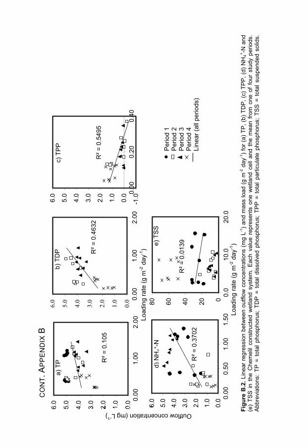
Figu

re B

.2. L

inea

r reg

ress

ion

betw

een

outfl

ow c

once

ntra

tions

(mg

L-1) a

nd m

ass

load

(g m

-2 d

ay-1

) for

(a) T

P, (b

) TD

P, (c

) TPP

, (d)

NH

4+ -N a

nd

(e)

TSS

in t

he C

hem

elil

cons

truct

ed w

etla

nd s

yste

m.

Each

val

ue r

epre

sent

s on

e w

etla

nd c

ell a

nd t

he m

ean

from

one

of

four

stu

dy p

erio

ds.

Abbr

evia

tions

: TP

= t

otal

pho

spho

rus;

TD

P =

tota

l dis

solv

ed p

hosp

horu

s; T

PP =

tot

al p

artic

ulat

e ph

osph

orus

; TS

S =

tota

l sus

pend

ed s

olid

s.

R² =

0.1

05

0.0

1.0

2.0

3.0

4.0

5.0

6.0 0.

001.

002.

00

a) T

P

R² =

0.4

632

0.0

1.0

2.0

3.0

4.0

5.0

6.0 0.

001.

002.

00

b) T

DP

R² =

0.5

495

-1.00.0

1.0

2.0

3.0

4.0

5.0

6.0 0.

000.

200.

40

c) T

PP

R² =

0.3

702

0.0

1.0

2.0

3.0

4.0

5.0

6.0 0.

000.

501.

001.

50

d) N

H4+ -

N

R² =

0.0

139

020406080

0.0

10.0

20.0

e) T

SS

CO

NT.

AP

PE

ND

IX B

Load

ing

rate

(g m

-2 d

ay-1

)

Load

ing

rate

(g m

-2 d

ay-1

)

0.0

1.0

2.0

3.0 2.0

3.0

4.0

5.0

6.0

Outflow concentration (mg L-1

)

Per

iod

1 P

erio

d 2

Per

iod

3 P

erio

d 4

Line

ar (a

ll pe

riods

)

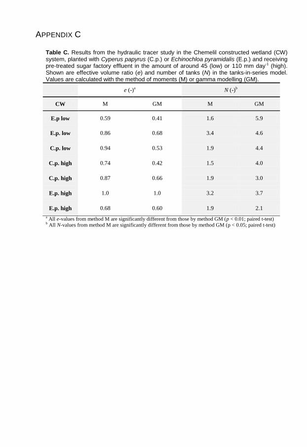
Table C. Results from the hydraulic tracer study in the Chemelil constructed wetland (CW) system, planted with Cyperus papyrus (C.p.) or Echinochloa pyramidalis (E.p.) and receiving pre-treated sugar factory effluent in the amount of around 45 (low) or 110 mm day-1 (high). Shown are effective volume ratio (e) and number of tanks (N) in the tanks-in-series model. Values are calculated with the method of moments (M) or gamma modelling (GM).

e (-)a N (-)

b

CW M GM M GM

E.p low 0.59 0.41 1.6 5.9

E.p. low 0.86 0.68 3.4 4.6

C.p. low 0.94 0.53 1.9 4.4

C.p. high 0.74 0.42 1.5 4.0

C.p. high 0.87 0.66 1.9 3.0

E.p. high 1.0 1.0 3.2 3.7

E.p. high 0.68 0.60 1.9 2.1

a All e-values from method M are significantly different from those by method GM (p < 0.01; paired t-test)

b All N-values from method M are significantly different from those by method GM (p < 0.05; paired t-test)

APPENDIX C

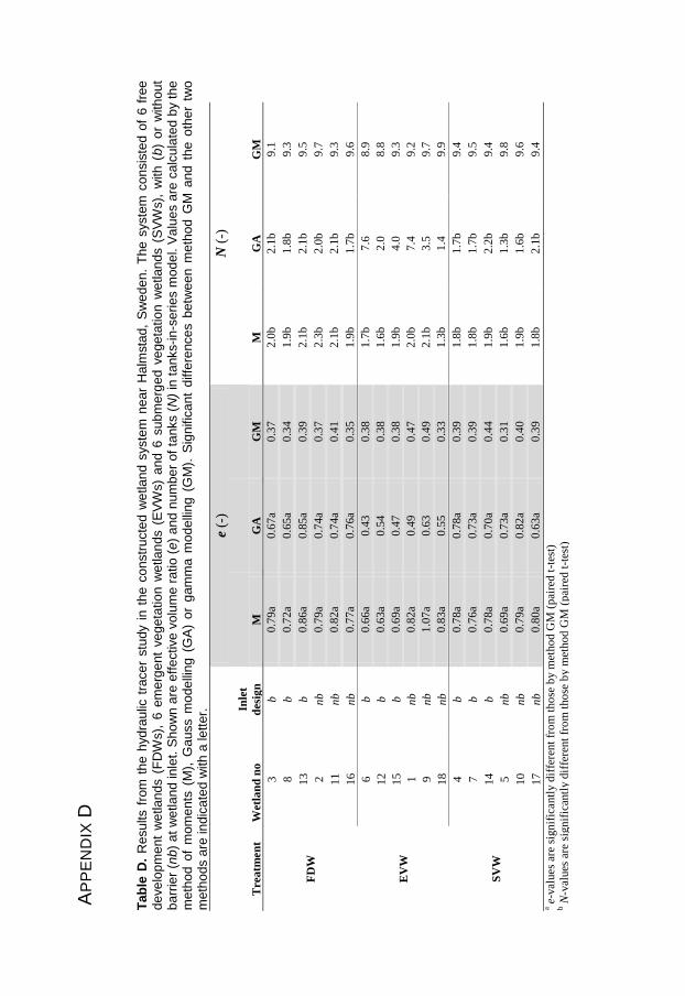
Ta

ble

D.

Re

sults f

rom

th

e h

yd

rau

lic t

racer

stu

dy i

n t

he c

onstr

ucte

d w

etlan

d s

yste

m n

ea

r H

alm

sta

d,

Sw

ede

n.

Th

e s

yste

m c

onsis

ted o

f 6

fre

e

deve

lopm

ent

we

tlan

ds (

FD

Ws),

6 e

me

rge

nt

ve

ge

tatio

n w

etlan

ds (

EV

Ws)

and

6 s

ubm

erg

ed v

ege

tatio

n w

etlan

ds (

SV

Ws),

with

(b)

or

with

ou

t b

arr

ier

(nb)

at

we

tlan

d in

let.

Sh

ow

n a

re e

ffe

ctive

vo

lum

e r

atio (

e)

and

num

ber

of

tanks (

N)

in t

anks-in-s

eries m

ode

l. V

alu

es a

re c

alc

ula

ted

by t

he

m

eth

od

of

mom

ents

(M

), G

auss m

ode

llin

g (

GA

) o

r g

am

ma

mo

de

llin

g (

GM

). S

ign

ific

ant

diffe

rence

s b

etw

een

me

tho

d G

M a

nd

th

e o

the

r tw

o

me

tho

ds a

re in

dic

ate

d w

ith

a le

tter.

e

(-)

N (

-)

Tre

atm

en

t W

etla

nd

no

Inle

t

des

ign

M

G

A

GM

M

G

A

GM

FD

W

3

b

0.7

9a

0.6

7a

0.3

7

2.0

b

2.1

b

9.1

8

b

0.7

2a

0.6

5a

0.3

4

1.9

b

1.8

b

9.3

13

b

0.8

6a

0.8

5a

0.3

9

2.1

b

2.1

b

9.5

2

nb

0.7

9a

0.7

4a

0.3

7

2.3

b

2.0

b

9.7

11

nb

0.8

2a

0.7

4a

0.4

1

2.1

b

2.1

b

9.3

16

nb

0.7

7a

0.7

6a

0.3

5

1.9

b

1.7

b

9.6

EV

W

6

b

0.6

6a

0.4

3

0.3

8

1.7

b

7.6

8

.9

12

b

0.6

3a

0.5

4

0.3

8

1.6

b

2.0

8

.8

15

b

0.6

9a

0.4

7

0.3

8

1.9

b

4.0

9

.3

1

nb

0.8

2a

0.4

9

0.4

7

2.0

b

7.4

9

.2

9

nb

1.0

7a

0.6

3

0.4

9

2.1

b

3.5

9

.7

18

nb

0.8

3a

0.5

5

0.3

3

1.3

b

1.4

9

.9

SV

W

4

b

0.7

8a

0.7

8a

0.3

9

1.8

b

1.7

b

9.4

7

b

0.7

6a

0.7

3a

0.3

9

1.8

b

1.7

b

9.5

14

b

0.7

8a

0.7

0a

0.4

4

1.9

b

2.2

b

9.4

5

nb

0.6

9a

0.7

3a

0.3

1

1.6

b

1.3

b

9.8

10

nb

0.7

9a

0.8

2a

0.4

0

1.9

b

1.6

b

9.6

17

nb

0.8

0a

0.6

3a

0.3

9

1.8

b

2.1

b

9.4

a e-v

alues

are

sig

nif

icantl

y d

iffe

rent

fro

m t

ho

se b

y m

etho

d G

M (

pai

red

t-t

est)

b N

-val

ues

are

sig

nif

ican

tly d

iffe

rent

fro

m t

ho

se b

y m

etho

d G

M (

pai

red

t-t

est)

AP

PE

ND

IX D