The Cryosphere, 9, 647–661, 2015

www.the-cryosphere.net/9/647/2015/

doi:10.5194/tc-9-647-2015

© Author(s) 2015. CC Attribution 3.0 License.

Warming permafrost and active layer variability

at Cime Bianche, Western European Alps

P. Pogliotti1, M. Guglielmin2, E. Cremonese1, U. Morra di Cella1, G. Filippa1, C. Pellet3, and C. Hauck3

1Environmental Protection Agency of Valle d’Aosta, Saint Christophe, Italy2Department of Theoretical and Applied Sciences, Insubria University, Varese, Italy3Department of Geosciences, University of Fribourg, Fribourg, Switzerland

Correspondence to: P. Pogliotti (paolo.pogliotti@gmail.com)

Received: 17 June 2014 – Published in The Cryosphere Discuss.: 21 July 2014

Revised: 21 February 2015 – Accepted: 10 March 2015 – Published: 8 April 2015

Abstract. The objective of this paper is to provide a first syn-

thesis on the state and recent evolution of permafrost at the

monitoring site of Cime Bianche (3100 m a.s.l.) on the Italian

side of the Western Alps. The analysis is based on 7 years of

ground temperature observations in two boreholes and seven

surface points. The analysis aims to quantify the spatial and

temporal variability of ground surface temperature in rela-

tion to snow cover, the small-scale spatial variability of the

active layer thickness and current temperature trends in deep

permafrost.

Results show that the heterogeneity of snow cover thick-

ness, both in space and time, is the main factor controlling

ground surface temperatures and leads to a mean range of

spatial variability (2.5± 0.1 ◦C) which far exceeds the mean

range of observed inter-annual variability (1.6± 0.1 ◦C). The

active layer thickness measured in two boreholes at a dis-

tance of 30 m shows a mean difference of 2.0± 0.1 m with

the active layer of one borehole consistently deeper. As re-

vealed by temperature analysis and geophysical soundings,

such a difference is mainly driven by the ice/water content in

the sub-surface and not by the snow cover regimes. The anal-

ysis of deep temperature time series reveals that permafrost

is warming. The detected trends are statistically significant

starting from a depth below 8 m with warming rates between

0.1 and 0.01 ◦C yr−1.

1 Introduction

The study of permafrost in mountain regions has become

relevant in view of ongoing climate changes (Stoffel et al.,

2014; Allen and Huggel, 2013; Etzelmüller, 2013; Fischer

et al., 2013; Haeberli, 2013; Harris et al., 2009; Gruber and

Haeberli, 2007; Gruber, 2004). Although permafrost warm-

ing and increasing active layer thickness (ALT) has been

observed worldwide (Harris, 2003; Smith et al., 2010; Ro-

manovsky et al., 2010; Wu and Zhang, 2008; Christiansen

et al., 2010; Guglielmin and Cannone, 2012; Guglielmin

et al., 2014a), in mountain areas the complexity of topog-

raphy, ground surface type, snow cover distribution, subsur-

face hydrology and geology strongly influence the thermal

regime of mountain permafrost (Gruber and Haeberli, 2009),

altering the response to changing environmental conditions.

For monitoring the huge spatial variability of mountain

permafrost, a number of monitoring sites has been estab-

lished through the Alps during the last years (e.g., Cremonese

et al., 2011). At present the collection of temperatures in

boreholes provides the best direct evidence of permafrost

state and evolution. Nevertheless, the combination of geo-

physical methods and thermal monitoring is particularly suit-

able for long-term monitoring of mountain permafrost be-

cause it provides crucial information on ground ice/water

content and structure (e.g., Hilbich et al., 2008; Haeberli

et al., 2010; PERMOS, 2013). The site of Cime Bianche

has been designed with the main objective of monitoring the

spatial variability of mountain permafrost. Moreover Cime

Bianche site is a permanent observatory in the southern side

of the European Alps, a region where permafrost observa-

Published by Copernicus Publications on behalf of the European Geosciences Union.

648 P. Pogliotti et al.: Warming permafrost and active layer variability

tions are more sparse and younger compared to the north-

ern side (e.g., Cremonese et al., 2011), and where significant

climatological differences occur (e.g., Frei and Schär, 1998;

Evans and Cox, 2005).

At Cime Bianche, the spatial variability of ground sur-

face temperature (GST) is measured because it has crucial

implications on the initialization, calibration and validation

of numerical models (e.g., Guglielmin et al., 2003; Noetzli

and Gruber, 2009; Hipp et al., 2014), and it is often used

as an indicator of permafrost occurrence. One of the main

challenges in the study of GST variability is the quantifi-

cation of the thermal effect of snow cover given the influ-

ence that it can have on thermal regime trough different pro-

cesses (Zhang, 2005; Luetschg et al., 2008; Guglielmin et al.,

2014b). On gentle slopes, snow cover mostly causes a net

increase of mean annual ground temperature due to the in-

sulating effect during winter, but timing of onset and melt-

out, duration, thickness and interaction with ground surface

characteristics strongly control the local magnitude of this ef-

fect (Hoelzle et al., 2003; Brenning et al., 2005; Gruber and

Hoelzle, 2008; Pogliotti, 2010; Gubler et al., 2011; Rödder

and Kneisel, 2012). Although a number of studies focused

on snow–GST interaction exists (e.g., Zhang, 2005, for a re-

view), little is known on its spatial and temporal variability

especially over complex alpine terrains.

Beside the GST, the active layer thickness is also mea-

sured at Cime Bianche. The World Meteorological Organi-

zation recognizes permafrost and active layer as one of the

essential climate variables selected for quantifying the im-

pacts of climate change (e.g., Harris and Haeberli, 2001). In

the Alps, the active layer is of particular interest because it di-

rectly affects slope processes (e.g., Fischer et al., 2012) and

infrastructures stability (e.g., Bommer et al., 2010; Spring-

man and Arenson, 2008). The active layer dynamics are con-

trolled by a number of variables such as air temperature, solar

radiation, topography, ground surface characteristics, ground

ice/water content and the timing, distribution and physical

characteristics of the snow cover (Zhang, 2005; Luetschg

et al., 2008; Scherler et al., 2010; Wollschläger et al., 2010;

Zenklusen Mutter and Phillips, 2012). As a consequence, the

active layer thickness has an high spatial and temporal vari-

ability (Anisimov et al., 2002; Wright et al., 2009) which in

the Alps may occur at very small scale.

Compared to the active layer which responds more to

short-term variations like seasonal snow and air tempera-

ture conditions, the deep (10 to 200 m) thermal regime of

permafrost reacts to long-term changes in climate (Beltrami,

2002). The deep permafrost temperature regime is a sensitive

indicator of the long-term climate variability and changes of

the surface energy balance (Romanovsky et al., 2002). The

trend analysis of deep temperature time series allows the de-

tection of signals of past and ongoing changes of permafrost

(e.g., Isaksen et al., 2001).

The overall objective of this paper is to provide a first syn-

thesis on the state and recent evolution of permafrost at Cime

Figure 1. Overview of the Cime Bianche monitoring site.

Bianche. In particular we present (i) the spatial and temporal

variability of GST and its relation with snow cover (ii) the

small-scale (30 m) ALT differences and (iii) the warming

trend of deep permafrost temperature.

2 Data and methods

2.1 Site description

The Cime Bianche monitoring site is located in the Western

Alps at the head of the Valtournenche valley (Valle d’Aosta,

Italy, 45◦55′ N–7◦41′ E) on the Italian side of the Matter-

horn, at 3100 m a.s.l. (Fig. 1). The site is located on a small

plateau slightly westward, with degrading characterized by

terracettes, convexities and depressions that result in a high

spatial variability of snow cover thickness during winter.

The bedrock lithology is homogeneous, mainly consisting

of garnetiferous micaschists and calcschists belonging to the

upper part of the Zermatt–Saas ophiolite complex (Dal Piaz,

1992). The bedrock surface is highly weathered and frac-

tured, locally resulting in a cover of coarse-debris deposits

with a thickness ranging from few centimeters to a couple

of meters. The presence of small landforms like gelifluc-

tion lobes (between 0.6 and almost 5 m in length) and sorted

polygons of fine material (with diameters ranging between

0.6 and 3.4 m) suggests the presence of permafrost.

The climate of the area is slightly continental. The long-

term mean annual precipitation is reported to be about

1000 mm yr−1 for the period 1931–1996 (Mercalli and Cat

Berro, 2003) while the in situ records show a mean of

1200 mm yr−1 for the period 2010–2013. The mean annual

air temperature (MAAT) is about −3.2 ◦C (mean 1951–

2011). Mean monthly air temperatures are positive from June

to September, while February and July are, respectively, the

coldest and the warmest months. The site is very windy and

mainly influenced by NE–NW air masses. The wind action

The Cryosphere, 9, 647–661, 2015 www.the-cryosphere.net/9/647/2015/

P. Pogliotti et al.: Warming permafrost and active layer variability 649

strongly contributes to the high spatial variability of snow

cover thickness.

Permafrost research in the area started in the late 1990s

(Guglielmin and Vannuzzo, 1995) with repeated campaigns

of measurements of the bottom temperature of snow (BTS)

and glaciological observations showing that the monitoring

site was probably ice covered during the climax of the Little

Ice Age. In 2003, as a preliminary investigations for site se-

lection, the potential permafrost occurrence in the area was

assessed using results from BTS, vertical electrical sound-

ings and ERT (electrical resistivity tomography) and the ap-

plication of numerical models like Permakart (Keller, 1992)

and Permaclim (Guglielmin et al., 2003).

2.2 Instrumentation

The site instrumentation started in 2005 and has been pro-

gressively upgraded during the following years. The current

setting is nearly unchanged since August 2008 and consists

of two boreholes, a spatial grid of ground surface tempera-

tures measures and an automatic weather station (AWS).

2.2.1 Boreholes

A deep (DP) and a shallow (SH) borehole, reaching a depth

of 41 and 6 m, respectively, located at a distance of about

30 m (Fig. 1), have been drilled in 2004 with core-destruction

method. Both boreholes are 127 mm in diameter with a

60 mm sealed PVC pipe for sensor housing. The boreholes

are equipped with thermistor chains based on resistors type

YSI 44031 (resolution 0.01 ◦C, absolute accuracy ±0.1 ◦C).

The entire setup (thermistor chains attached to the data log-

ger) have been calibrated by the manufacturer before the in-

stallation. Sensors depths in meters from the surface are 0.02,

0.3, 0.6, 1, 1.6, 2, 2.3, 2.6, 3, 3.3, 3.6, 4, 4.6, 5.9 for SH

and 0.02, 0.3, 0.6, 1, 1.6, 2, 2.6, 3, 3.6, 4, 6, 8, 10, 12, 14, 15,

16, 17, 18, 20, 25, 30, 35, 40, 41 for DP. In each borehole,

the shallower sensors (0.02 and 0.3 m) are cabled on two in-

dependent chains and are used to measure the ground sur-

face temperature outside the PVC tube in order to avoid the

thermal disturbance of the casing. Temperatures are sampled

every 10 min and recorded by a Campbell Scientific CR800

data logger. The system is equipped with a GPRS module for

daily remote data transmission.

2.2.2 Ground surface temperature grid (GSTgrid)

A small grid (40 m× 10 m) is used for monitoring the spatial

variability of GST. The grid consists of five nodes: four at the

corners and one in the center (Fig. 1). Each node is equipped

with two platinum resistors, PT1000 (resolution 0.01 ◦C, ac-

curacy ±0.1 ◦C), buried in the ground at depths of 0.02 and

0.3 m (according to Guglielmin, 2006). Ground temperatures

are recorded hourly by a Geoprecision D-Log12 data logger.

For the analysis, GST measured at the two boreholes is

also included; thus data from seven nodes are used for the

analysis. Ground surface at each node is mainly character-

ized by coarse debris with a fine matrix of coarse sand and

fine gravel. At each node, the sensors are placed in the ma-

trix thus local ground conditions are nearly homogeneous

between all nodes. In contrast, snow cover depth and du-

ration sharply differ across the grid nodes. For this reason,

based on field observations and temperature time series anal-

ysis (Schmid et al., 2012) the data set is divided in snow-

free and snow-covered nodes. The first group includes three

nodes characterized by shallow or intermittent winter snow

cover, while the latter group includes four nodes that clearly

show a long lasting deep snow cover damping temperature

oscillations during winter (Fig. 1).

2.2.3 Automatic weather station

An AWS has been installed just above the borehole SH since

2006. Air temperature and relative humidity, atmospheric

pressure, wind speed and direction, incoming and outgo-

ing short- and long-wave solar radiation and snow depth are

recorded every 10 min by a Campbell Scientific CR3000 data

logger. The system is equipped with a GPRS module for the

daily remote data transmission. In September 2011 a second

snow depth sensor was installed in the surroundings of the

DP borehole. Finally, solid and liquid precipitation has been

measured since January 2009 by an OTT Pluvio2 system.

2.3 Data analysis

This section reports a short description of the methods used

for the calculations of synthesis parameters considered in this

study.

MAGT is the mean annual ground temperature at a specific

depth (m) (e.g., MAGT10).

MAGST is the mean annual ground surface temperature.

ALT is the active layer thickness defined as the maximum

depth (m) reached by the 0 ◦C isotherm at the end of the

warm season. It is calculated considering the maximum daily

temperature at each sensor depth and interpolating between

the deepest sensor with positive value and the sensor beneath.

The maximum of the resulting vector and the corresponding

day are named ALT and ALTday, respectively. This proce-

dure is applied on the warmest period of the year, here fixed

from 1 August to 30 November. The uncertainty of ALT es-

timation is evaluated considering the amplitude of thermis-

tors noise (inferred from calibration of the manufacturer) and

the interpolation distance between the sensors. Considering

these factors, the uncertainty of ALT estimation is ±0.15 m

in borehole SH and ±0.2 m in borehole DP.

TTOP is the MAGT at the top of the permafrost table

(Smith and Riseborough, 1996). It is calculated by interpola-

tion of the MAGT at depth of the ALT that is considering the

first sensors above and below the ALT.

THO is the thermal offset within the active layer and is

computed as TTOP-MAGST (Burn and Smith, 1988).

www.the-cryosphere.net/9/647/2015/ The Cryosphere, 9, 647–661, 2015

650 P. Pogliotti et al.: Warming permafrost and active layer variability

Figure 2. Example of detection of snow cover duration from GST

time series with the method of Schmid et al. (2012). OD is the on-

set date of snow; MD is the melting date of snow. The periods used

for the calculation of MAGST, SD and MAATsf are represented by

the scheme on top.

Zero annual amplitude oscillation (ZAA) is the depth

beneath which there is almost no annual fluctuation (AF)

in ground temperature, nominally smaller than 0.1 ◦C (van

Everdingen, 2005). The AF is calculated at each sensor depth

as the difference between annual maximum and annual mini-

mum of the mean daily temperatures. The ZAA is calculated

by interpolation between the deepest sensor with AF greater

than 0.1 ◦C and the sensor beneath. When necessary, a mov-

ing average, with a window of 360 days, is applied on deep

nodes data (below 8 m) before daily aggregation to remove

electrical noise (±0.01 ◦C).

All the parameters listed above, with the exception of ALT,

are computed considering the hydrological year (beginning

1 October) as a reference period. All the analyses are per-

formed with the free statistical software R (R Core Team,

2014). When appropriate, the variability of the results is ex-

pressed in terms of standard error (se= sd/√

n, where se is

standard error, sd is standard deviation and n is the sample

size).

2.4 Snow cover duration and snow-free days

In order to investigate the effect of snow cover duration and

air temperature on MAGST, the method of Schmid et al.

(2012) is applied on snow-covered nodes using the sensors at

0.02 m. This method allows us to infer the date of snow onset

(OD) and the date of snow melt (MD) from the amplitude of

ground temperature oscillation. Subsequently, starting from

OD and MD, it is possible to calculate (i) the duration of

snow cover (SD, Fig. 2) as the number of days between OD

and MD and (ii) the number of snow-free days as the sum of

remaining days of autumn and summer. The latter period is

used as reference for calculating the mean annual air temper-

ature of snow-free days (MAATsf, Fig. 2).

Figure 3. Methodological steps of trend analysis. Step 1: monthly

aggregation (thin black line with circles). Step 2: seasonal detrend-

ing (thick black line). Step 3: trend fitting (dashed red line). Vertical

dashed lines represents 1 October, materializing the limits of the

hydrological years.

2.5 Trend analysis

In order to look for linear trends that might reflect warming,

two non-parametric methods are applied to borehole tem-

peratures: Mann–Kendall test (MK) (Mann, 1945; Kendall,

1948) and Sen’s slope estimator (SS) (Sen, 1968). These

methods are commonly used to assess trends and related

significance levels in hydro-meteorological time series such

as water quality, stream flow, temperature and precipitation

(e.g., Gocic and Trajkovic, 2013; Kousari et al., 2013). The

reason for using non-parametric statistical tests is that they

are more suitable for non-normally distributed data and are

not sensitive to outliers or abrupt changes.

The procedure chosen includes (i) the pre-whitening of

the data to remove the lag-1 autocorrelation components as

recommended by von Storch and Navarra (1999) (see also

Hamed, 2009 and Bence, 1995), (ii) the fitting of the trend’s

slope with SS and (iii) the testing of trend significance level

(p value) with MK. Such a procedure is implemented in the

R package zyp (Bronaugh et al., 2013).

Given the short climatological time span of the borehole

observations, a seasonal detrending is recommended, as sug-

gested by Helsel and Hirsch (1992), for better discerning the

long-term linear trend over time. Thus, a seasonal decompo-

sition based on loess smoother (Cleveland, 1979; Cleveland

et al., 1990) is applied to the monthly aggregated time se-

ries of each borehole before applying SS and MK (Fig. 3).

Such a seasonal detrending method is implemented by the R

function stl (R Core Team, 2014).

2.6 Geophysics

At the end of summer 2013, two geophysical surveys have

been realized with the objective to assess the composition of

The Cryosphere, 9, 647–661, 2015 www.the-cryosphere.net/9/647/2015/

P. Pogliotti et al.: Warming permafrost and active layer variability 651

the subsurface. A first, explorative geoelectric (ERT) profile

was performed on 16 August 2013 and repeated on 9 Oc-

tober 2013 in combination with one refraction seismic to-

mography (RST) along the same line (see Fig. 1). Combining

refraction seismic and ERT measurements enables us to un-

ambiguously identify the subsurface materials in the ground.

Due to very different specific resistivities, ERT is best suited

to differentiate between ice and water, whereas the distinc-

tion between air and ice can more easily be accomplished

by RST because of large contrasts between their respective

p wave velocities.

2.6.1 Electrical Resistivity Tomography

A 94 m long electrode array composed of 48 electrodes with

2 m spacing was installed along a straight line less than 2 m

away from the two boreholes (Fig. 1). Current was injected

using varying electrode pairs, and the resulting potential dif-

ferences were automatically measured by a Syscal (Iris In-

struments) for each quadrupole possible with the Wenner–

Schlumberger configuration (529 measurements, 23 depth

levels). The electrode locations were marked with spray paint

and a number of electrodes were left on site to facilitate fur-

ther measurements.

The measured apparent resistivity data sets were then in-

verted using the RES2DINV software (Geotomosoft, 2014)

with the following setup. A robust inversion constraint was

applied to avoid unrealistic smoothing of the calculated spe-

cific resistivities. Additionally, the depth of the model layers

was increased by a factor 1.5 and an extended model was

used to match the model grid of the corresponding seismic

inversion. Note that for geometric reasons, the two lower cor-

ners of the resulting tomograms have very low sensitivity to

the obtained data and should not be over-interpreted. Finally,

a time-lapse inversion scheme was applied to the two ERT

data sets, yielding the percentage of resistivity change from

the first measurements to the second. Here, an unconstraint

inversion was chosen, meaning that the ERT measurements

were inverted independently.

2.6.2 Refraction seismic tomography

The measurements were conducted using a Geode seis-

mometer (Geometrics) and 24 geophones placed with 4 m

spacing. A seismic signal was generated in-between every

second geophone pair by repeatedly hitting a steel plate with

a sledge hammer. To improve the signal-to-noise ratio, the

signal was stacked at least 15 times at each location. Two ad-

ditional offset shot points were measured (3 m before the first

geophone and 6 m beyond the last one) in order to maximize

the spatial resolution and match the ERT profile length and

depth of investigation.

The first arrivals of the seismic p wave were manually

picked for each seismogram using the software REFLEXW

(Sandmeier, 2014). A simultaneous iterative reconstruction

Figure 4. Mean annual ground surface temperatures at depths of

0.02 m (red) and 0.3 m (blue). Star symbols indicate snow-covered

nodes, while bullets indicate snow-free nodes. The horizontal lines

indicate the mean MAGST for each year and each depth. Black rect-

angles are used to highlight the min–max envelope to facilitate the

inter-annual comparison.

technique algorithm was then used to reconstruct a 2-D to-

mogram of p wave velocity distribution based on the ob-

tained travel times. Starting from a synthetic model, the

travel times are calculated and compared to the measured

ones. The model is then updated iteratively by minimizing

the residuals between measured and calculated travel times.

3 Results

3.1 Ground surface temperatures

Figure 4 shows MAGST at 0.02 and 0.3 m on the seven

GST nodes. Some years (e.g., 2009, 2011, 2013) show

a MAGST spatial variability, evaluated as the range of

MAGST measured in all nodes and greater than 3 ◦C, that

clearly exceeds the inter-annual variability. In general, con-

sidering all 7 years, we observed that mean spatial variabil-

ity (2.5± 0.1 ◦C) is greater than mean inter-annual variabil-

ity (1.6± 0.1 ◦C). The results are similar at both depth. The

difference between MAGST measured at 0.02 and 0.3 m is,

on average, 0.4± 0.1 ◦C, with deeper sensors usually warmer

than the shallower ones. On average, the thermal offset due

to snow cover is about 1.5± 0.2 ◦C with snow-covered nodes

being warmer than snow-free nodes. These observations con-

firm that the warming and cooling effects of, respectively, a

thick and thin snow cover (Zhang, 2005; Pogliotti, 2010) can

coexist over short distances (< 50 m) and lead to high spatial

variability of the GST.

www.the-cryosphere.net/9/647/2015/ The Cryosphere, 9, 647–661, 2015

652 P. Pogliotti et al.: Warming permafrost and active layer variability

Figure 5. Scatterplots of SD (a) and MAATsf (b) against MAGST. The solid line represents the linear fit while the dotted lines are the

confidence intervals. The metrics of the fitting are also reported.

The duration of snow (SD) on snow-covered nodes is on

average 270± 6 days with a mean range of spatial variabil-

ity of 28 days and a mean range of inter-annual variability of

48 days. To disentangle the influence of snow and air tem-

perature on surface temperature in snow-covered nodes, we

tested the relationship between MAGST and MAAT and be-

tween MAATsf and SD. We found no significant correlation

between MAGST and MAAT. Figure 5 shows the scatterplot

comparing SD (A), MAATsf (B) and MAGST: MAGST is

significantly correlated to both SD (p < 0.05) and MAATsf

(p < 0.001), with the latter explaining the higher portion of

variance (R2= 0.39). Being computed on snow-free days,

MAATsf is mainly controlled by air temperature but partially

also by the duration of snow cover, therefore integrating the

relative contribution of both components (snow duration and

air temperature) on MAGST.

3.2 Active layer

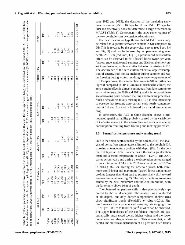
Table 1 summarizes the active layer parameters observed in

the two boreholes. Since August 2008 data are available at

both SH and DP boreholes, results of ALT can be compared

over 6 years while MAGST, TTOP and THO over 5 years

(shaded rows in Table 1). Missing values (column % NA) in

both boreholes are lower than 4 % in all years.

ALT is the parameter showing the greater difference be-

tween the two boreholes with a mean of 2.7± 0.3 m in SH

and 4.7± 0.2 m in DP. The mean inter-annual difference of

ALT between the two boreholes is 2.0± 0.1 m, while the

mean absolute inter-annual variability of ALT at borehole

level is 1.0± 0.1 m. In both boreholes the maximum ALT

has been recorded in 2012 and the minimum in 2010. ALT

(date) is normally anticipated in DP (except 2013) with dif-

ferences ranging from a few days (e.g., 2009) to more than

3 weeks (e.g., 2012). The MAGST is on average slightly

lower in SH, which normally shows a thinner winter snow

Figure 6. Fluctuations of snow cover thickness (Hs) and ground

temperatures (daily mean) at selected depths in the active layers

of Cime Bianche from 1 October 2010 to 30 September 2013 de-

termined from borehole temperature data. Lines type: dashed is

for SH, solid is for DP. Colors: red is for shallower temperatures

(1.6 m), blu is for deeper temperature (3 m), grey is for snow.

cover compared to DP (Fig. 6). The TTOP values are very

similar, around −0.9 ◦C. The THO is negative in both bore-

holes (except 2013) with a mean value of about −0.5 ◦C in

DP and −0.3 ◦C in SH.

The values of Table 1 show that all the active layer pa-

rameters are very similar between the two boreholes with the

only exception of ALT, which in DP is nearly double than

in SH. To better understand the causes of this difference,

the daily mean temperatures at selected depths within the

active layer of both boreholes and the corresponding snow

cover thickness are compared in Fig. 6. Although a consis-

tently thinner snow depth is recorded on SH compared to

DP (mean difference ∼ 41± 14 cm during the winter sea-

The Cryosphere, 9, 647–661, 2015 www.the-cryosphere.net/9/647/2015/

P. Pogliotti et al.: Warming permafrost and active layer variability 653

Tab

le1.

Sy

nth

esis

par

amet

ers

of

acti

ve

lay

ers

reco

rded

inth

etw

ob

ore

ho

les

of

Cim

eB

ian

che.

Th

eav

erag

eval

ues

(Av

g.)

are

calc

ula

ted

over

the

per

iod

20

09

–2

01

3w

her

ed

ata

fro

m

bo

thb

ore

ho

les

are

avai

lab

le.

Acr

ony

ms:

hy

dro

log

ical

yea

r(H

.Y

.),

acti

ve

lay

erth

ick

nes

s(A

LT

),m

ean

ann

ual

gro

un

dsu

rfac

ete

mp

erat

ure

(MA

GS

T),

mea

nan

nu

alte

mp

erat

ure

atth

e

top

of

per

maf

rost

(MA

PT

),th

erm

alo

ffse

t(T

HO

FF

),m

issi

ng

dat

a(N

A),

shal

low

bo

reh

ole

(SH

),d

eep

bo

reh

ole

(DP

).

H.Y

.A

LT

(m)

AL

T(d

ate)

MA

GS

T(◦

C)

MA

PT

(◦C

)T

HO

FF

(◦C

)%

NA

SH

DP

SH

DP

SH

DP

SH

DP

SH

DP

SH

DP

2006

3.1

–11

Oct

––

––

––

––

–

2007

2.4

–14

Oct

–−

0.3

–−

0.8

–−

0.4

–0

–

2008

1.9

3.9

27

Sep

25

Sep

−2.1

–−

1.8

–0.3

–4.3

8–

2009

3.0

4.9

24

Oct

20

Oct

−0

0−

0.7

−0.8

−0.6

−0.9

3.2

83.2

8

2010

1.9

3.8

18

Oct

8O

ct−

1.1

−1.2

−1.2

−1.3

−0.1

−0.1

1.3

71.3

7

2011

3.3

5.1

8N

ov

23

Oct

−0.5

0.1

−1.1

−1

−0.6

−1.1

0.2

70

2012

3.6

5.4

30

Oct

4O

ct−

0.4

−0.3

−0.8

−0.7

−0.4

−0.5

2.7

43.0

1

2013

2.0

4.6

13

Oct

13

Oct

−1.3

−0.7

−1

−0.6

0.3

0.1

3.6

3.5

9

Avg.

2.7±

0.3

4.7±

0.2

24

Oct

13

Oct

−0.7±

0.2−

0.4±

0.2

−1±

0.1−

0.9±

0.1

2−

0.3±

0.2−

0.5±

0.2

2.2

5±

0.6

22.2

5±

0.6

8

sons 2012 and 2013), the duration of the insulating snow

cover is similar (250± 16 days for SH vs. 254± 17 days for

DP) and effectively does not determine a large difference in

MAGST (Table 1). Consequently, the snow cover regimes of

the two boreholes can be considered equivalent.

For these reasons we hypothesize that ALT difference may

be related to a greater ice/water content in SH compared to

DP. This is revealed by the geophysical survey (see Sect. 3.4

and Fig. 9) and can be inferred by temperatures at greater

depth. At 1.6 m (red lines, Fig. 6) a pronounced zero-curtain

effect can be observed in SH (dashed lines) twice per year,

(i) from snow melt to mid-summer and (ii) from the snow on-

set to mid-winter, while a similar behavior is missing in DP.

The occurrence of the zero-curtain reflects a large consump-

tion of energy, both for ice melting during summer and wa-

ter freezing during winter, resulting in lower temperatures of

SH. Deeper down, the summer heat wave in SH is further de-

layed if compared to DP: at 3 m in SH (dashed blue lines) the

zero-curtain effect is almost continuous from late summer to

early winter (e.g., in 2010 and 2011), and it is not possible to

see a breaking point between melting and freezing processes.

Such a behavior is totally missing in DP. It is also interesting

to observe that freezing zero-curtain ends nearly contempo-

rary at 1.6 and 3 m and is followed by a rapid temperature

drop.

In conclusion, the ALT at Cime Bianche shows a pro-

nounced spatial variability probably caused by the variability

of ice/water content in the sub-surface and associated energy

consumption resulting from freezing and melting processes.

3.3 Permafrost temperature and warming trend

Due to the small depth reached by the borehole SH, the anal-

ysis of permafrost temperature is limited to the borehole DP.

Looking at temperature profiles with depth (Fig. 7), the per-

mafrost layer at Cime Bianche has a thickness greater than

40 m and a mean temperature of about −1.2 ◦C. The ZAA

varies across years and during the observation period ranged

from a minimum of 14.2 m in 2011 to a maximum of 16.2 m

in 2013 (Table 2). During the observed years, both mini-

mum (solid lines) and maximum (dashed lines) temperature

profiles (deeper than 6 m) tend to progressively shift toward

warmer temperatures (Fig. 7). The only exceptions are repre-

sented by the 2011 maximum and the 2009 minimum, with

the latter only above 10 m of depth.

The observed temperature shift is also quantitatively sup-

ported by the trend analysis. The analysis was conducted

at all depths, but only deeper temperatures (below 8 m)

show significant trends (Kendall’s p value < 0.01). Fig-

ure 8 reveals that a pronounced warming rate ranging from

0.1 ◦C yr−1 at 8 m to 0.007 ◦C yr−1 at 41 m can be observed.

The upper boundaries of the confidence intervals are sys-

tematically unbalanced toward higher values and the lower

boundaries are always above zero. This means that, at all

depths, the statistical distribution of all possible fitted trends

www.the-cryosphere.net/9/647/2015/ The Cryosphere, 9, 647–661, 2015

654 P. Pogliotti et al.: Warming permafrost and active layer variability

Figure 7. Minimum (solid lines) and maximum (dashed lines) tem-

perature profiles in the borehole DP below 6 m of depth for the pe-

riod 2009–2013.

is positively skewed. Based on this analysis, it is concluded

that permafrost at Cime Bianche is warming because signifi-

cant positive warming rates are reported below 8 m.

3.4 Geophysics

Figure 9 shows the final distribution of specific resistivity for

the two ERT measurements, the percentage of change in the

model resistivity between the two time steps and the p wave

velocity distribution over the same subsection. Additionally,

the surface characteristics and a detailed analysis of the geo-

physical properties at the two borehole locations (SH and DP,

Fig. 10) are included in the analysis.

The overall characteristics of both ERT profiles are very

similar (Fig. 9a and b) and can be divided into three main

zones: a low resistive layer directly below the surface, vary-

ing between 2.5 m thickness at the top of the slope and 7 m

thickness at the bottom; two high resistive areas with val-

ues exceeding 20 000 �m, located below the superficial layer

(from the start of the subsection to the superficial borehole:

0–34 m and 40–52 m); and a less-high resistive area on the

lower part of the profile below 5 m depth.

Comparing the two ERT data sets (cf. also the time-lapse

image in Fig. 9c), one can observe a clear increase of the

uppermost low resistive layer between August and October

which is coherent with a thickening of the active layer ob-

served in the borehole temperature during this period. An-

other main difference between the two measurements is the

apparition of two low resistive zones at 34 and 60 m, visi-

ble down to 10 and 15 m depth, respectively. These areas can

also be seen in the ERT tomogram from August but much

Table 2. Interpolated depth of zero annual amplitude oscillation

(ZAA) and corresponding mean temperatures in the borehole DP.

H. Y. ZAA (1T = 0.1 ◦C)

Depth (m) Temp. (◦C)

2009 15.5 −1.3

2010 15.2 −1.2

2011 14.2 −1.3

2012 15.3 −1.2

2013 16.2 −1.2

Avg. 15.3 −1.2

Figure 8. Warming rate calculated over the period 2009–2013 be-

low 8 m of depth in the borehole DP as a function of depth. Black

dots represent linear trends as ◦C yr−1. The uncertainty of trend

values is represented by the dashed bars, which indicate the lower

and upper boundaries of the 95 % confidence interval of the fitting

model (see Sect. 2.5 for details).

less developed and limited to a few meters. In addition, the

very high resistive area located in the upper part of the pro-

file is much smaller and displaced by about 5 m towards the

lower part of the profile in the second measurement.

These changes are clearly visible in blue (increase) and

red (decrease) colors in Fig. 9c. As stated before, the two

data sets were inverted independently within the time-lapse

scheme. A constrained inversion (results not shown here)

would yield very similar overall distribution of resistivity

changes; the only difference is a much smaller range of val-

ues. The large area of resistivity increase, located just above

the superficial borehole location and reaching down to the

The Cryosphere, 9, 647–661, 2015 www.the-cryosphere.net/9/647/2015/

P. Pogliotti et al.: Warming permafrost and active layer variability 655

Figure 9. Tomograms of the specific resistivities for both ERT measurements: (a) 16 August 2013, (b) 9 October 2013, (c) percentage

change in model resistivity between the two dates and (d) seismic velocities. The location of SH and DP is figured with vertical black lines

of respective length. A rough description of the surface aspect along the profile is also shown (e).

bottom of the profile, corresponds to the displacement of the

high resistive area observed in the ERT tomograms.

The RST tomogram exhibits much less lateral variations

than the ERT results (see Fig. 9d), pointing to the influence

of liquid water in the ERT results. One can clearly see a rela-

tively slow layer with velocities between 300 and 1500 m s−1

(red and dark red colors) just below the surface, with vary-

ing thickness between 3 and 5 m. This layer is thickest in

the vicinity of SH and thinnest at DP (64 m). Below this first

layer the velocities increase steadily until reaching the max-

imum (around 6400 m s−1). The rate of velocity increase is

strongest around 40 m and there is a clear distinction between

the upper part of the profile (until 45 m) and the lower one. At

depth the high velocity zone is present in the upper part and

not in the lower part of the profile. Conversely, the velocities

at the surface are much higher in the lower part (especially

around DP) than in the upper part.

Both geophysical profiles show clear differences in the

subsurface properties as well as surface composition at the

borehole locations (Fig. 9e). The upper part of the profile (un-

til 50 m) is more or less homogeneously covered by medium

size blocks and has the deepest layer of coarse-debris de-

posits, whereas the granulometry in the lower part is much

more variable at the surface and the debris layer is thinner.

The boreholes are located in very different conditions: DP is

located in-between two zones composed of big blocks (from

pluridecimetric to metric), whereas SH is located at the junc-

tion between medium size blocks (from pluricentimetric to

decimetric), mixed and non-mixed with soil. To relate in de-

tail the results yielded by the geophysics and the measured

temperature, the vertical distribution of specific resistivity,

seismic velocity and ground temperature at SH and DP are

shown in Fig. 10.

4 Discussion

4.1 Ground surface temperatures

In this study both the inter-annual and the spatial vari-

ability of MAGST within a restricted area has been ana-

lyzed and compared: the results show that at Cime Bianche,

the mean range of spatial variability (2.5± 0.1 ◦C) far ex-

ceeds the mean range of observed inter-annual variability

(1.6± 0.1 ◦C). Given the comparatively homogeneous char-

acteristics of the ground surface at the sensors locations, such

a variability is essentially caused by the heterogeneity of the

snow cover thickness both in space (effect of wind redis-

tribution and micro-morphology) and time (effect of vari-

able weather conditions and precipitations). In particular,

the combination of snow cover duration and air temperature

during the snow-free period is the main factor controlling

MAGST values. This is true not only for snow-free nodes

but also for nodes experiencing long-lasting (270 days) yet

highly variable (28 days) snow cover.

The thermal effect of snow cover on ground surface

temperature has been extensively analyzed (e.g., Goodrich,

1982; Keller and Gubler, 1993; Zhang, 2005; Luetschg et al.,

2008; Langer et al., 2013). In recent years, with the advances

of minilogger technology, the number of field experiments

aimed at the characterization of the spatial variability of GST

has grown. Recently Gubler et al. (2011) observed a spatial

variability of more than 2.5 ◦C within a number of square

www.the-cryosphere.net/9/647/2015/ The Cryosphere, 9, 647–661, 2015

656 P. Pogliotti et al.: Warming permafrost and active layer variability

Figure 10. Vertical distribution of specific resistivity and P wave velocity at the borehole locations, extracted from the tomograms shown

in Fig. 9, as well as borehole temperatures for the dates of the ERT and RST measurements. The horizontal lines represent the active layer

thickness at the respective time periods.

homogeneous areas of 10× 10 m. In Norway, Isaksen et al.

(2011) report that MAGST varied by 1.5–3.0 ◦C over dis-

tances of 30–100 m in a region characterized by mountain

permafrost. Rödder and Kneisel (2012) observed ranges ex-

ceeding 4.3 ◦C between adjacent loggers (< 50 m), although

this value includes inhomogeneities of surface characteris-

tics. Similar results were obtained by Gisnås et al. (2014),

who observed a variability of the MAGST of up to 6 ◦C

within heterogeneous areas of 0.5 km2.

The inter-annual variability of MAGST caused by snow

is also well known and documented by a number of studies

(Romanovsky et al., 2003; Hoelzle et al., 2003; Karunaratne

and Burn, 2004; Brenning et al., 2005; Etzelmüller, 2007;

Ødegård and Isaksen, 2008; Schneider et al., 2012) but has

rarely been explicitly analyzed and quantified. An exception

in the Alps is represented by Hoelzle et al. (2003), who re-

ported an inter-annual variability of ±2.7 ◦C measured dur-

ing two seasons on eight mini-loggers with different surface

characteristics in the Murtèl–Corvatsch area. Our results thus

report a more robust quantification of the mean inter-annual

GST variability (1.6± 0.12 ◦C), based on a longer time series

(7 years).

The obtained results are very similar at both measurement

depths. Given such a small difference and the agreement of

temperature fluctuations between 2 and 30 cm, it is arguable

that to describe the spatial variability of GST and run long-

term GST observations, measurements at two or more depths

are not needed.

4.2 Active layer

In this study, both ALT and temperature fluctuations within

the active layer of two adjacent boreholes have been com-

pared. Such experimental design provides direct evidence of

the small-scale spatial variability of the ALT and allows to

evaluate the effect of ice/water content on sub-surface tem-

perature.

From 2009 to 2013 the ALT at Cime Bianche varied

within 2.0 and 5.5 m with a mean inter-annual variability

of 1.0± 0.1 m. These ranges and the observed inter-annual

variability of ALT are comparable to those recorded in

other alpine sites (Anisimov et al., 2002; Christiansen, 2004;

Schneider et al., 2012; Smith et al., 2010; PERMOS, 2013)

In the Swiss Alps, the thickness of the active layer typi-

cally varies between 0.5 and 8 m depth (Gruber and Haeberli,

2009; PERMOS, 2009, 2013).

ALT in the borehole SH is systematically lower than in

DP (mean difference 2.0± 0.1 m) even though all the ac-

tive layer parameters (MAGST, TTOP, THO see Table 1)

are very similar between the two boreholes. On one hand,

such a similarity suggests that snow cover regimes above

the two boreholes are nearly equivalent; thus snow proba-

bly plays a major role only on the inter-annual variability

of ALT. On the other hand, the pronounced spatial variabil-

ity of ALT is probably caused by the variability of ice/water

content in the sub-surface and associated variation of energy

consumption resulting from freezing and melting processes.

Langer et al. (2013) confirms this hypothesis by observing,

in a tundra lowland landscape, that ALT is related mainly

to ground properties (ice content), whereas snow physical

The Cryosphere, 9, 647–661, 2015 www.the-cryosphere.net/9/647/2015/

P. Pogliotti et al.: Warming permafrost and active layer variability 657

properties have greatest influence on the ground surface tem-

peratures. Probably the different ice/water content between

SH and DP is caused by snowmelt and meltwater infiltration

along preferential discontinuities (a borehole acts a discon-

tinuity itself). Hilbich et al. (2008) observed at Schilthorn

(Swiss Alps) a similar situation between two boreholes 15 m

apart, ascribing the lower ALT of one borehole to the higher

moisture contents (and related freezing) caused by preferen-

tial water flow paths from the surrounding slopes. Schneider

et al. (2012) analyzed the thermal regime of four adjacent

boreholes drilled on differing material (coarse debris, fine

debris and bedrock) at Murtèl–Corvatsch (Swiss Alps) and

recognized meltwater and ice content as mainly responsible

for the observed ALT spatial variability.

The different amount of available water in the active layer

of the two boreholes is also reflected by the occurrence of

the zero-curtain in the borehole SH and its absence in the

borehole DP. In the upper part of the active layer, a pro-

nounced zero-curtain can be observed two times per year:

(i) from snow melt to mid-summer (spring zero-curtain) and

(ii) from the snow onset to mid-winter (autumn zero-curtain).

Recently, Zenklusen Mutter and Phillips (2012) deeply an-

alyzed similar behaviors on a sample of 10 boreholes in

Switzerland, observing that, on average, the duration of the

spring zero-curtain is usually shorter than the autumn one

and is strongly dependent on snow depth at the end of the

winter. At Cime Bianche, such a distinction between spring

and autumn zero-curtain is not always possible in the deeper

part of the active layer. As also observed by Rist and Phillips

(2005), it may happen that, below a certain depth, the ground

temperature does not become positive because the energy

from the summer heat wave is not sufficient to melt all ice

before the onset of the subsequent winter season. This con-

tinuous zero-curtain is more probable when a higher amount

of meltwater is available (Scherler et al., 2010; Kane et al.,

2001) and can occur at a different depth from year to year,

strongly influencing the resulting ALT.

4.3 Permafrost temperature and warming trend

In order to look for trends that might reflect warming, two

non-parametric methods were applied to borehole tempera-

ture time series. The detected linear trends are statistically

significant (Kendall’s p value < 0.01) only at depth below

8 m. Probably, in the first meters, the seasonal and inter-

annual variability of temperatures is so strong that signifi-

cant trends are not detectable, although a seasonal detrend-

ing being applied to remove such high-frequency oscillations

(see also Sect. 2.5). The detected trends span the range 0.1–

0.01 ◦C yr−1, suggesting that at Cime Bianche permafrost is

warming.

As also discussed by Zenklusen Mutter et al. (2010), the

detection of trends on time series covering a short time span

requires caution and adoption of specific criteria. Moreover,

the estimation of uncertainties and significance levels is also

fundamental for facilitating the comparisons of trends be-

tween differing sites and for reproducing trend detection

methods on others data sets.

Permafrost warming trends have been observed world-

wide, both at high latitude (Harris, 2003; Osterkamp, 2005;

Smith et al., 2005; Osterkamp, 2007; Isaksen et al., 2007;

Farbrot et al., 2013; Jonsell et al., 2013) and at lower latitude

in high mountains (Vonder Mühll, 2001; Harris, 2003; Gru-

ber, 2004; Wu and Zhang, 2008; Phillips and Mutter, 2009;

Zenklusen Mutter et al., 2010; PERMOS, 2013; Haeberli,

2013).

Recently in the Alps, Zenklusen Mutter et al. (2010)

detected trends on daily temperature time series of two

boreholes in the Muot da Barba Peider ridge (Eastern

Swiss Alps). For the deep frozen bedrock between 8 and

17.5 m, a general warming trend was found with significant

(p value < 0.05) values ranging from 0.042 to 0.025 ◦C yr−1.

At Cime Bianche a similar range of warming rate was found

between 16 and 20 m. The substantial difference between the

two sites is that the Swiss boreholes are drilled at the top of

a NW-oriented ridge with a mean slope of 38◦ and thus have

a strong 3-D thermal effect induced by topography (Noet-

zli et al., 2007). In the mountains of Scandinavia, Isaksen

et al. (2007) reported warming trends between 20 and 60 m

of depth ranging from about 0.05 to 0.005 ◦C yr−1 over three

sites, while Isaksen et al. (2011) found an increase in mean

ground temperature between 6 and 9 m of depth at two sites,

with rates ranging from about 0.015 to 0.095 ◦C yr−1. Re-

cently at Tarfala mountain station (Sweden), Jonsell et al.

(2013) found trends over 11 years (2001–2011) ranging from

0.047 to 0.002 ◦C yr−1 between 20 and 100 m of depth.

The absolute values of warming rates are difficult to com-

pare because of different site characteristics, geographical

regions and methods used for trend detection. Nevertheless,

some similitudes exist between our and the above-mentioned

case studies: (i) trends are difficult to detect at shallower

depth because of the higher seasonal variability of temper-

atures; (ii) warming trends are mainly significant below 8–

10 m of depth; (iii) warming trends exponentially decrease

with depth; (iv) there is no evidence of negative (cooling)

trends at any depth in recent literature.

4.4 Geophysics

Given the relatively high resistivity and p wave velocities

along the profiles, the presence of permafrost observed in

the borehole data is confirmed by the geophysics over the

whole profile length (Fig. 9). Moreover, a clear discrepancy

between the upper part of the profile where SH is located and

the lower one with borehole DP can be seen in both the ERT

and the RST data.

At DP, the comparatively high p wave velocities indi-

cate the presence of weathered bedrock close to the surface,

whereas at SH a layer of coarse-debris deposits in the up-

permost 5 m is confirmed by very low p wave velocities.

www.the-cryosphere.net/9/647/2015/ The Cryosphere, 9, 647–661, 2015

658 P. Pogliotti et al.: Warming permafrost and active layer variability

Conversely, p wave velocities at depth are higher for SH

(around ∼ 6000 m s−1) than for DP (around ∼ 5000 m s−1,

see also Fig. 10). This difference, also seen in the resistiv-

ity data (around 17 000 � m at SH and 13 000 � m at DP),

would indicate that a larger ice content is present in the ups-

lope part of the profile than in the lower part. This is in good

agreement with the spatial variation of ALT highlighted in

Sect. 3.2 and the zero-curtain phase observed only at SH (see

Fig. 6).

The low-resistivity and low-velocity layer near the surface,

the thickness of which increases visibly between August and

October in the ERT data, is considered to be the active layer.

Figure 10 compares the vertical distribution of specific elec-

trical resistivity, p wave velocity and temperature for both

boreholes and dates. At first glance, there seems to be a mis-

match between resistivity and temperature regarding ALT for

SH. However, borehole temperatures at SH in August show

constant values at the freezing point between 1 and 3 m depth

(between 2 and 4 m in October), the deeper level being the

depth of the sharply increasing resistivity values. As resis-

tivity is sensitive to the liquid water content, its values will

not increase significantly before most of this liquid water has

been frozen, coinciding with a temperature increase to val-

ues below the freezing point (e.g., Hauck, 2002). Due to the

higher water/ice content in SH, this phenomenon (∼ vertical

zero-curtain) is only seen in SH and not in DP.

The two low resistive areas (34–40 and 53–60 m), already

visible in August and more pronounced on the second ERT

profile in October, are interpreted as the preferential water

flow path. Since the melt water cannot infiltrate through the

two ice-rich (high resistive) bodies close by (at 20–33 and

40–52 m horizontal distances), it is forced to follow a prefer-

ential path in-between. The lower infiltration area (53–60 m)

is constrained in the upper part by the ice-rich zone and in

the lower part by the presence of bedrock near the surface.

Finally, the displacement of the high resistive area ob-

served near SH (blue zone at depth on the time-lapse tomo-

gram) is most likely an inversion artefact (overcompensation)

due to the appearance of the low resistive area in the second

ERT profile (cf. Hilbich et al., 2009).

5 Conclusions

This paper presents a first synthesis on the thermal state

and recent evolution of permafrost in the monitoring site of

Cime Bianche, one of the few permanent observatories on the

southern side of the European Alps. The analysis focused on

(i) the spatial and temporal variability of MAGST in relation

to snow cover, (ii) the small-scale (30 m) spatial variability

of ALT and (iii) the warming rate of deep permafrost tem-

peratures. The results of analysis show the following:

1. Spatial variability of MAGST is greater than its inter-

annual variability and is controlled by a combination of

air temperature during the snow-free period and snow

duration.

2. The ALT at Cime Bianche has a pronounced spatial

variability caused mainly by a different ice/water con-

tent due to very different surface and subsurface condi-

tions in terms of weathering and fracturing of bedrock.

3. Permafrost at Cime Bianche is warming at significant

rates below 8 m of depth.

The Supplement related to this article is available online

at doi:10.5194/tc-9-647-2015-supplement.

Acknowledgements. This work has been co-funded by a grant from

Ev-K2-CNR.

The authors are grateful to the lift company Cervino S.p.a for the

continuous logistical support to the research activities at the moni-

toring site of Cime Bianche.

C. Pellet and C. Hauck gratefully acknowledge a grant from

the Swiss National Science Foundation (project SOMOMOUNT

No. 200021_143325).

Edited by: J. Boike

References

Allen, S. K. and Huggel, C.: Extremely warm temperatures as a

potential cause of recent high mountain rockfall, Global Planet.

Change, 107, 59–69, doi:10.1016/j.gloplacha.2013.04.007,

2013.

Anisimov, O., Shiklomanov, N., and Nelson, F.: Variability of sea-

sonal thaw depth in permafrost regions: a stochastic model-

ing approach, Ecol. Model., 153, 217–227, doi:10.1016/S0304-

3800(02)00016-9, 2002.

Beltrami, H.: Climate from borehole data: Energy fluxes and

temperatures since 1500, Geophys. Res. Lett., 29, 2111,

doi:10.1029/2002GL015702, 2002.

Bence, J. R.: Analysis of short time series: correcting for autocorre-

lation, Ecology, 76, 628–639, 1995.

Bommer, C., Phillips, M., and Arenson, L. U.: Practical recommen-

dations for planning, constructing and maintaining infrastruc-

ture in mountain Permafrost, Permafrost Periglac., 21, 97–104,

doi:10.1002/ppp.679, 2010.

Brenning, A., Gruber, S., and Hoelzle, M.: Sampling and statistical

analyses of BTS measurements, Permafrost Periglac., 16, 383–

393, doi:10.1002/ppp.541, 2005.

Bronaugh, D., Werner, A., and For the Pacific Climate Impacts

Consortium: zyp: Zhang+Yue-Pilon trends package, available

at: http://cran.r-project.org/package=zyp (last access: July 2014),

2013.

Burn, C. and Smith, C.: Observations of the “Thermal Offset”

in near-surface mean annual ground temperatures at several

sites near Mayo, Yukon Territory, Canada, Arctic, 41, 99–104,

doi:10.14430/arctic1700, 1988.

The Cryosphere, 9, 647–661, 2015 www.the-cryosphere.net/9/647/2015/

P. Pogliotti et al.: Warming permafrost and active layer variability 659

Christiansen, H. H.: Meteorological control on interannual spa-

tial and temporal variations in snow cover and ground thaw-

ing in two northeast Greenlandic Circumpolar-Active-Layer-

Monitoring(CALM) sites, Permafrost Periglac., 15, 155–169,

doi:10.1002/ppp.489, 2004.

Christiansen, H. H., Etzelmüller, B., Isaksen, K., Juliussen, H.,

Farbrot, H., Humlum, O., Johansson, M., Ingeman-Nielsen, T.,

Kristensen, L., Hjort, J., and Others, A.: The thermal state

of permafrost in the nordic area during the international

polar year 2007–2009, Permafrost Periglac., 21, 156–181,

doi:10.1002/ppp.687, 2010.

Cleveland, R., Cleveland, W., McRae, J. E., and Terpenning, I.:

STL: A seasonal-trend decomposition procedure based on loess,

J. Official Stat., 6, 3–73, 1990.

Cleveland, W.: Robust locally weighted regression and

smoothing scatterplots, J. Am. Stat. Assoc., 74, 829–836,

doi:10.1080/01621459.1979.10481038, 1979.

Cremonese, E., Gruber, S., Phillips, M., Pogliotti, P., Boeckli, L.,

Noetzli, J., Suter, C., Bodin, X., Crepaz, A., Kellerer-Pirklbauer,

A., Lang, K., Letey, S., Mair, V., Morra di Cella, U., Ravanel, L.,

Scapozza, C., Seppi, R., and Zischg, A.: Brief Communication:

“An inventory of permafrost evidence for the European Alps”,

The Cryosphere, 5, 651–657, doi:10.5194/tc-5-651-2011, 2011.

Dal Piaz, G. V.: Le Alpi dal M. Bianco al Lago Maggiore:

13 Itinerari Automobilistici e 97 Escursioni a Piedi, Vol. 1, Seven

Hills Books, Padova, Italy, 1992.

Etzelmüller, B.: The regional distribution of mountain per-

mafrost in Iceland, Permafrost Periglac., 199, 185–199,

doi:10.1002/ppp.583, 2007.

Etzelmüller, B.: Recent advances in mountain permafrost research,

Permafrost Periglac., 24, 99–107, doi:10.1002/ppp.1772, 2013.

Evans, I. S. and Cox, N. J.: Global variations of local asymmetry in

glacier altitude: separation of north–south and east–west compo-

nents, J. Glaciol., 51, 469–482, 2005.

Farbrot, H., Isaksen, K., Etzelmüller, B., and Gisnås, K.: Ground

thermal regime and permafrost distribution under a changing

climate in Northern Norway, Permafrost Periglac., 24, 20–38,

doi:10.1002/ppp.1763, 2013.

Fischer, L., Purves, R. S., Huggel, C., Noetzli, J., and Haeberli, W.:

On the influence of topographic, geological and cryospheric fac-

tors on rock avalanches and rockfalls in high-mountain areas,

Nat. Hazards Earth Syst. Sci., 12, 241–254, doi:10.5194/nhess-

12-241-2012, 2012.

Fischer, L., Huggel, C., Kääb, A., and Haeberli, W.: Slope fail-

ures and erosion rates on a glacierized high-mountain face un-

der climatic changes, Earth Surf. Proc. Land., 38, 836–846,

doi:10.1002/esp.3355, 2013.

Frei, C. and Schär, C.: A precipitation climatology of the alps

from high-resolution rain-gauge observations, Int. J. Climatol.,

18, 873–900, 1998.

Geotomosoft: Res2dinv software Tutorial: 2-D and 3-D electrical

imaging surveys, available at: www.geotomosoft.com, last ac-

cess: July 2014.

Gisnås, K., Westermann, S., Schuler, T. V., Litherland, T., Isaksen,

K., Boike, J., and Etzelmüller, B.: A statistical approach to rep-

resent small-scale variability of permafrost temperatures due to

snow cover, The Cryosphere, 8, 2063–2074, doi:10.5194/tc-8-

2063-2014, 2014.

Gocic, M. and Trajkovic, S.: Analysis of changes in meteorologi-

cal variables using Mann–Kendall and Sen’s slope estimator sta-

tistical tests in Serbia, Global Planet. Change, 100, 172–182,

doi:10.1016/j.gloplacha.2012.10.014, 2013.

Goodrich, L. E.: The influence of snow cover on the ground ther-

mal regime, Can. Geotech. J., 19, 421–432, doi:10.1139/t82-047,

1982.

Gruber, S.: Permafrost thaw and destabilization of Alpine rock walls

in the hot summer of 2003, Geophys. Res. Lett., 31, L13504,

doi:10.1029/2004GL020051, 2004.

Gruber, S. and Haeberli, W.: Permafrost in steep bedrock

slopes and its temperature related destabilization follow-

ing climate change, J. Geophys. Res.-Earth, 112, F02S18,

doi:10.1029/2006JF000547, 2007.

Gruber, S. and Haeberli, W.: Mountain permafrost, in: Permafrost

Soils, Springer, Innsbruck, Austria, 33–44, doi:10.1007/978-3-

540-69371-0, 2009.

Gruber, S. and Hoelzle, M.: The cooling effect of coarse blocks re-

visited: a modeling study of a purely conductive mechanism, in:

Proceedings of the 9th International Conference on Permafrost,

29 June–3 July 2008, Fairbanks, Alaska, USA, 557–561, 2008.

Gubler, S., Fiddes, J., Keller, M., and Gruber, S.: Scale-

dependent measurement and analysis of ground surface temper-

ature variability in alpine terrain, The Cryosphere, 5, 431–443,

doi:10.5194/tc-5-431-2011, 2011.

Guglielmin, M.: Ground surface temperature (GST), active layer

and permafrost monitoring in continental Antarctica, Permafrost

Periglac., 17, 133–143, doi:10.1002/ppp.553, 2006.

Guglielmin, M. and Cannone, N.: A permafrost warming

in a cooling Antarctica?, Climatic Change, 111, 177–195,

doi:10.1007/s10584-011-0137-2, 2012.

Guglielmin, M. and Vannuzzo, C.: Studio della distribuzione del

permafrost e delle relazioni con i ghiacciai della piccola età

glaciale nell’alta valtournenche (Valle d’Aosta, Italia), Atti Tici-

nesi di Scienze della Terra, 38, 119–127, 1995.

Guglielmin, M., Aldighieri, B., and Testa, B.: PERMACLIM:

a model for the distribution of mountain permafrost, based

on climatic observations, Geomorphology, 51, 245–257,

doi:10.1016/S0169-555X(02)00221-0, 2003.

Guglielmin, M., Dalle Fratte, M., and Cannone, N.: Permafrost

warming and vegetation changes in continental Antarctica, Env-

iron. Res. Lett., 9, 045001, doi:10.1088/1748-9326/9/4/045001,

2014a.

Guglielmin, M., Worland, M. R., Baio, F., and Convey, P.:

Permafrost and snow monitoring at Rothera Point (Adelaide

Island, Maritime Antarctica): implications for rock weath-

ering in cryotic conditions, Geomorphology, 225, 47–56,

doi:10.1016/j.geomorph.2014.03.051, 2014b.

Haeberli, W.: Mountain permafrost research frontiers and a spe-

cial long-term challenge, Cold Reg. Sci. Technol., 96, 71–76,

doi:10.1016/j.coldregions.2013.02.004, 2013.

Haeberli, W., Noetzli, J., Arenson, L. U., Delaloye, R., Gärtner-

Roer, I., Gruber, S., Isaksen, K., Kneisel, C., Krautblatter, M.,

and Phillips, M.: Mountain permafrost: development and chal-

lenges of a young research field, J. Glaciol., 56, 1043–1058,

doi:10.3189/002214311796406121, 2010.

Hamed, K.: Enhancing the effectiveness of prewhitening in

trend analysis of hydrologic data, J. Hydrol., 368, 143–155,

doi:10.1016/j.jhydrol.2009.01.040, 2009.

www.the-cryosphere.net/9/647/2015/ The Cryosphere, 9, 647–661, 2015

660 P. Pogliotti et al.: Warming permafrost and active layer variability

Harris, C.: Warming permafrost in European moun-

tains, Global Planet. Change, 39, 215–225,

doi:10.1016/j.gloplacha.2003.04.001, 2003.

Harris, C. and Haeberli, W.: Permafrost monitoring in the high

mountains of Europe: the PACE project in its global context, Per-

mafrost Periglac., 11, 3–11, doi:10.1002/ppp.377, 2001.

Harris, C., Arenson, L. U., Christiansen, H. H., Etzelmüller, B.,

Frauenfelder, R., Gruber, S., Haeberli, W., Hauck, C., Höl-

zle, M., Humlum, O., Isaksen, K., Kääb, A., Kern-Lütschg, M.,

Lehning, M., Matsuoka, N., Murton, J., Nötzli, J., Phillips, M.,

Ross, N., Seppälä, M., Springman, S., and Vonder Mühll, D.: Per-

mafrost and climate in Europe: monitoring and modelling ther-

mal, geomorphological and geotechnical responses, Earth-Sci.

Rev., 92, 117–171, doi:10.1016/j.earscirev.2008.12.002, 2009.

Hauck, C.: Frozen ground monitoring using DC resis-

tivity tomography, Geophys. Res. Lett., 29, 12-1–12-4,

doi:10.1029/2002GL014995, 2002.

Helsel, D. R. and Hirsch, R. M.: Trend analysis, in: Statistical Meth-

ods in Water Resources, chap. 12, Elsevier, Amsterdam, Holland,

1992.

Hilbich, C., Hauck, C., Hoelzle, M., Scherler, M., Schudel, L.,

Völksch, I., Vonder Mühll, D., and Mäusbacher, R.: Monitoring

mountain permafrost evolution using electrical resistivity tomog-

raphy: a 7-year study of seasonal, annual, and long-term varia-

tions at Schilthorn, Swiss Alps, J. Geophys. Res., 113, F01S90,

doi:10.1029/2007JF000799, 2008.

Hilbich, C., Marescot, L., Hauck, C., Loke, M.H. and Mäus-

bacher, R.: Applicability of Electrical Resistivity Tomography

Monitoring to coarse blocky and ice-rich permafrost landforms,

Permafrost Periglac., 20, 269–284, 2009.

Hipp, T., Etzelmüller, B., and Westermann, S.: Permafrost in

Alpine Rock faces from Jotunheimen and Hurrungane, Southern

Norway, Permafrost Periglac., 25, 1–13, doi:10.1002/ppp.1799,

2014.

Hoelzle, M., Haeberli, W., and Stocker-Mittaz, C.: Miniature

ground temperature data logger measurements 2000–2002 in

the Murtèl-Corvatsch area, Eastern Swiss Alps, in: Proceed-

ings of the 8th International Conference on Permafrost, 1, 7–12,

available at: http://www.geo.uzh.ch/~hoelzle/hoelzleetal2003b.

pdf (last access: July 2014), 2003.

Isaksen K., Holmlund, P., Sollid, J. L., and Harris, C.: Three deep

alpine-permafrost boreholes in svalbard and scandinavia, Per-

mafrost Periglac., 12, 13–25, 2001.

Isaksen, K., Sollid, J. L., Holmlund, P., and Harris, C.: Recent

warming of mountain permafrost in Svalbard and Scandinavia, J.

Geophys. Res., 112, F02S04, doi:10.1029/2006JF000522, 2007.

Isaksen, K., Ødegård, R. S., Etzelmüller, B., Hilbich, C., Hauck, C.,

Farbrot, H., Eiken, T., Hygen, H. O., and Hipp, T. F.: Degrading

mountain permafrost in Southern Norway: spatial and temporal

variability of mean ground temperatures, 1999–2009, Permafrost

Periglac., 22, 361–377, doi:10.1002/ppp.728, 2011.

Jonsell, U., Hock, R., and Duguay, M.: Recent air and ground tem-

perature increases at Tarfala Research Station, Sweden, Polar

Res., 1, 1–11, available at: http://www.polarresearch.net/index.

php/polar/article/view/19807 (last access: July 2014), 2013.

Kane, D. L., Hinkel, K. M., Goering, D. J., Hinzman, L. D.,

and Outcalt, S. I.: Non-conductive heat transfer associ-

ated with frozen soils, Global Planet. Change, 29, 275–292,

doi:10.1016/S0921-8181(01)00095-9, 2001.

Karunaratne, K. C. and Burn, C. R.: Relations between air and

surface temperature in discontinuous permafrost terrain near

Mayo, Yukon Territory, Can. J. Earth Sci., 1451, 1437–1451,

doi:10.1139/E04-082, 2004.

Keller, F.: Automated mapping of mountain permafrost using

the program PERMAKART within the geographical infor-

mation system ARC/INFO, Permafrost Periglac., 3, 133–138,

doi:10.1002/ppp.3430030210, 1992.

Keller, F. and Gubler, H. U.: Interaction between snow cover and

high mountain permafrost, Murtel-Corvatsch, Swiss Alps, in:

vol. 1, Proceedings of the Sixth International Conference on

Permafrost, Beijing, 21–25 July, Zurich, Switzerland, 332–337,

1993.

Kendall, M. G.: Rank Correlation Methods, Griffin, Oxford, Eng-

land, 1948.

Kousari, M. R., Ahani, H., and Hendi-zadeh, R.: Temporal

and spatial trend detection of maximum air temperature in

Iran during 1960–2005, Global Planet. Change, 111, 97–110,

doi:10.1016/j.gloplacha.2013.08.011, 2013.

Langer, M., Westermann, S., Heikenfeld, M., Dorn, W., and

Boike, J.: Satellite-based modeling of permafrost temperatures

in a tundra lowland landscape, Remote Sens. Environ., 135, 12–

24, doi:10.1016/j.rse.2013.03.011, 2013.

Luetschg, M., Lehning, M., and Haeberli, W.: A sensitivity study

of factors influencing warm/thin permafrost in the Swiss Alps,

J. Glaciol., 54, 696–704, doi:10.3189/002214308786570881,

2008.

Mann, H. B.: Nonparametric tests against trend, Econometrics, 13,

245–259, 1945.

Mercalli, L. and Cat Berro, D.: Atlante Climatico Della Valle

d’Aosta, Vol. 2, SMS, Oxford, England, 2003.

Noetzli, J. and Gruber, S.: Transient thermal effects in Alpine per-

mafrost, The Cryosphere, 3, 85–99, doi:10.5194/tc-3-85-2009,

2009.

Noetzli, J., Gruber, S., Kohl, T., Salzmann, N., and Haeberli, W.:

Three-dimensional distribution and evolution of permafrost tem-

peratures in idealized high-mountain topography, J. Geophys.

Res., 112, F02S13, doi:10.1029/2006JF000545, 2007.

Ødegård, R. and Isaksen, K.: MAGST in mountain permafrost,

Dovrefjell, southern Norway, 2001–2006, in: Proceedings of

the 9th International Conference on Permafrost, 1311–1315,

available at: https://www.matnat.uio.no/geo/english/research/

projects/cryolink/publications/NICOPoedegaardetal.pdf (last ac-

cess: July 2014), 2008.

Osterkamp, T. E.: The recent warming of permafrost

in Alaska, Global Planet. Change, 49, 187–202,

doi:10.1016/j.gloplacha.2005.09.001, 2005.

Osterkamp, T. E.: Characteristics of the recent warming of

permafrost in Alaska, J. Geophys. Res., 112, F02S02,

doi:10.1029/2006JF000578, 2007.

PERMOS: Permafrost in Switzerland 2004/2005 and 2005/2006,

Glaciological Report Permafrost No. 6/7, Tech. Rep. 6,

Cryospheric Commission of the Swiss Academy of Sciences,

Zurich, Switzerland, 2009.

PERMOS: Permafrost in Switzerland 2008/2009 and 2009/2010,

Glaciological Report Permafrost No. 10/11, Tech. Rep. 10,

Cryospheric Commission of the Swiss Academy of Sciences,

Zurich, Switzerland, 2013.

The Cryosphere, 9, 647–661, 2015 www.the-cryosphere.net/9/647/2015/

P. Pogliotti et al.: Warming permafrost and active layer variability 661

Phillips, M. and Mutter, E.: Rapid degradation of ground ice in

a ventilated talus slope: flüela Pass, Swiss Alps, Permafrost

Periglac., 14, 1–14, doi:10.1002/ppp.638, 2009.

Pogliotti, P.: Influence of Snow Cover on MAGST over Complex

Morphologies in Mountain Permafrost Regions, PhD thesis, Uni-

versity of Turin, Turin, Italy, 2010.

R Core Team: R: A Language and Environment for Statistical Com-

puting, R Foundation for Statistical Computing, Vienna, Austria,

available at: http://www.r-project.org/, last access: July 2014.

Rist, A. and Phillips, M.: First results of investigations on hy-

drothermal processes within the active layer above alpine per-

mafrost in steep terrain, Norsk Geogr. Tidsskr., 59, 177–183,

doi:10.1080/00291950510020574, 2005.

Rödder, T. and Kneisel, C.: Influence of snow cover and grain

size on the ground thermal regime in the discontinuous per-

mafrost zone, Swiss Alps, Geomorphology, 175–176, 176–189,

doi:10.1016/j.geomorph.2012.07.008, 2012.

Romanovsky, V. E., Burgess, M., Smith, S., Yoshikawa, K.,

and Brown, J.: Permafrost temperature records: indicators

of climate change, EOS T. Am. Geophys. Un., 83, 589,

doi:10.1029/2002EO000402, 2002.

Romanovsky, V. E., Sergueev, D. O., and Osterkamp, T. E.: Tem-

poral variations in the active layer and near-surface permafrost

temperatures at the long-term observatories in northern Alaska,

Month, 8, Proceedings of the 8th International Conference on

Permafrost, 21–25 July, Zurich, Switzerland, 2003.

Romanovsky, V. E., Drozdov, D. S., Oberman, N. G.,

Malkova, G. V., Kholodov, A. L., Marchenko, S. S.,

Moskalenko, N. G., Sergeev, D. O., Ukraintseva, N. G.,

Abramov, A., Gilichinsky, D., and Vasiliev, A. A.: Thermal state

of permafrost in Russia, Permafrost Periglac., 21, 136–155,

doi:10.1002/ppp.683, 2010.

Sandmeier: ReflexW Scientific Software, Sandmeier geophysi-

cal research, available at: www.sandmeier-geo.de, last access:

2 April 2015, Karlsruhe, Germany, 2014.

Scherler, M., Hauck, C., Hoelzle, M., Stähli, M., and Völksch, I.:

Meltwater infiltration into the frozen active layer at an

alpine permafrost site, Permafrost Periglac., 21, 325–334,

doi:10.1002/ppp.694, 2010.

Schmid, M.-O., Gubler, S., Fiddes, J., and Gruber, S.: Inferring

snowpack ripening and melt-out from distributed measurements

of near-surface ground temperatures, The Cryosphere, 6, 1127–

1139, doi:10.5194/tc-6-1127-2012, 2012.

Schneider, S., Hoelzle, M., and Hauck, C.: Influence of surface and

subsurface heterogeneity on observed borehole temperatures at

a mountain permafrost site in the Upper Engadine, Swiss Alps,

The Cryosphere, 6, 517–531, doi:10.5194/tc-6-517-2012, 2012.

Sen, P. K.: Estimates of the regression coefficient based

on Kendall’s tau, J. Am. Stat. Assoc., 63, 1379–1389,

doi:10.1080/01621459.1968.10480934, 1968.

Smith, M. and Riseborough, D.: Permafrost monitoring and detec-

tion of climate change, Permafrost Periglac., 7, 301–309, 1996.

Smith, S. L., Burgess, M., Riseborough, D., and Mark Nixon, F.:

Recent trends from Canadian permafrost thermal mon-

itoring network sites, Permafrost Periglac., 16, 19–30,

doi:10.1002/ppp.511, 2005.

Smith, S. L., Romanovsky, V. E., Lewkowicz, A. G., Burn, C. R.,

Allard, M., Clow, G., Yoshikawa, K., and Throop, J.: Ther-

mal state of permafrost in North America: a contribution to

the international polar year, Permafrost Periglac., 21, 117–135,

doi:10.1002/ppp.690, 2010.

Springman, S. and Arenson, L. U.: Recent advances in permafrost

geotechnics, in: Proceedings of the 9th International Conference

on Permafrost, 29 June–3 July 2008, Fairbanks, Alaska, USA,

1685–1694, 2008.

Stoffel, M., Tiranti, D., and Huggel, C.: Climate change

impacts on mass movements – case studies from the

European Alps, Sci. Total Environ., 493, 1255–1266,

doi:10.1016/j.scitotenv.2014.02.102, 2014.

van Everdingen, R. O.: Multi-language glossary of permafrost and

related ground-ice terms, Tech. rep., International Permafrost As-

sociation, Boulder, Colorado, available at: https://nsidc.org/fgdc/

glossary/ (last access: July 2014), 2005.

von Storch, H. and Navarra, A.: Analysis of climate variability: ap-

plications of statistical techniques, Springer, Berlin, Germany,

1999.

Vonder Mühll, D.: Thermal variations of mountain permafrost: an

example of measurements since 1987 in the Swiss Alps, in:

Global Change and Protected Areas, Springer Netherlands, 83–

95, 2001.

Wollschläger, U., Gerhards, H., Yu, Q., and Roth, K.: Multi-channel

ground-penetrating radar to explore spatial variations in thaw

depth and moisture content in the active layer of a permafrost

site, The Cryosphere, 4, 269–283, doi:10.5194/tc-4-269-2010,

2010.

Wright, N., Hayashi, M., and Quinton, W. L.: Spatial and tempo-

ral variations in active layer thawing and their implication on

runoff generation in peat-covered permafrost terrain, Water Re-

sour. Res., 45, W05414, doi:10.1029/2008WR006880, 2009.

Wu, Q. and Zhang, T.: Recent permafrost warming on

the Qinghai-Tibetan Plateau, J. Geophys. Res., 113,

D13108,doi:10.1029/2007JD009539, 2008.

Zenklusen Mutter, E. and Phillips, M.: Active layer characteristics

at ten borehole sites in Alpine permafrost terrain, Switzerland,

Permafrost Periglac., 23, 138–151, doi:10.1002/ppp.1738, 2012.

Zenklusen Mutter, E., Blanchet, J., and Phillips, M.: Analy-

sis of ground temperature trends in Alpine permafrost us-

ing generalized least squares, J. Geophys. Res., 115, F04009,

doi:10.1029/2009JF001648, 2010.

Zhang, T.: Influence of the seasonal snow cover on the ground

thermal regime: an overview, Rev. Geophys., 43, RG4002,

doi:10.1029/2004RG000157, 2005.

www.the-cryosphere.net/9/647/2015/ The Cryosphere, 9, 647–661, 2015