HAL Id: hal-01576516https://hal.archives-ouvertes.fr/hal-01576516

Submitted on 23 Aug 2017

HAL is a multi-disciplinary open accessarchive for the deposit and dissemination of sci-entific research documents, whether they are pub-lished or not. The documents may come fromteaching and research institutions in France orabroad, or from public or private research centers.

L’archive ouverte pluridisciplinaire HAL, estdestinée au dépôt et à la diffusion de documentsscientifiques de niveau recherche, publiés ou non,émanant des établissements d’enseignement et derecherche français ou étrangers, des laboratoirespublics ou privés.

Walking on Gravel with Soft Soles using Linear InvertedPendulum Tracking and Reaction Force DistributionAdrien Pajon, Stéphane Caron, Giovanni de Magistris, Sylvain Miossec,

Abderrahmane Kheddar

To cite this version:Adrien Pajon, Stéphane Caron, Giovanni de Magistris, Sylvain Miossec, Abderrahmane Kheddar.Walking on Gravel with Soft Soles using Linear Inverted Pendulum Tracking and Reaction ForceDistribution. Humanoids, Nov 2017, Birmingham, United Kingdom. pp.432-437, �10.1109/HU-MANOIDS.2017.8246909�. �hal-01576516�

Walking on Gravel with Soft Soles using Linear Inverted PendulumTracking and Reaction Force Distribution

Adrien Pajon1, Stephane Caron1, Giovanni De Magistris2, Sylvain Miossec3 and Abderrahmane Kheddar1,4

Abstract— Soft soles absorb impacts and cast ground un-evenness during locomotion on rough terrains. However, theyintroduce passive degrees of freedom (deformations under thefeet) that complexify the tasks of state estimation and overallrobot stabilization. We address this problem by developing acontrol loop that stabilizes humanoid robots when walking withsoft soles on flat and uneven terrain. Our closed-loop controllerminimizes the errors on the center of mass (COM) and the zeromoment point (ZMP) with an admittance control of the feetbased on a simple deformation estimator. We demonstrate itseffectiveness in real experiments on the HRP-4 humanoid.

I. INTRODUCTION

Walking with rigid limbs and feet forces contact transitionsto be planned with nearly zero velocity to avoid shocks. Thisis a very conservative strategy that goes against dynamicmotion. In order to absorb shocks at impacts and lowertheir propagation along the mechanical structure, humanoidrobots integrate compliant mechanisms. A common solutionis to add flexible mechanisms at the robot ankles [1], [2]that also protect the force sensor at each foot. However,such compliant mechanisms act like passive joints whosedeformations [3] are not directly measurable. This makesthe control of robot attitude difficult notably in complexmaneuvers [4].

Rather than using compliant shock absorbers at the ankle,we investigate the use of thick soft soles under each foot,see early work in [5]. These soles absorb landing impactsand cast out ground unevenness, implying an increase ofthe contact surface. In order to generate a simulator of thedeformable soles, we developed a deformation estimator [6]coupled with a corresponding Walking Pattern Generator(WPG) [7]. This simulator has been experimentally vali-dated by successfully walking in open-loop with HRP-4performing different experiments [8]. However, its time-consuming computations prevented its application to onlinemotion generation.

In this paper we develop a closed-loop controller for bipedrobots walking with soft soles. The goal of this controlleris to minimize the tracking error in terms of COM velocity,COM and ZMP position by taking into account the deforma-tion properties of materials under the feet. This results intoan admittance control at the ankles whose gains are basedon the sole stiffness in a nominal state from the deformation

1 CNRS-UM2 LIRMM, IDH group, UMR5506, Montpellier, France.2 IBM Research - Tokyo, IBM Japan3 Univ. Orleans, INSA-CVL, PRISME, EA 4229, F45072, France4 CNRS-AIST Joint Robotics Laboratory (JRL), UMI3218/RL, Japan.Corresponding author: adrien.pajon@gmail.com

Fig. 1: Different views of HRP-4 walking on gravel with softsoles.

estimator. We tested our approach on a humanoid robot HRP-4 walking on gravel, as depicted in Figure 1.

II. CONTROL FRAMEWORK STRUCTURE

Our control pipeline is illustrated in Figure 2. Superscriptsd are used to denote desired references, c control referencesand i ∈ {R,L} right or left foot references. This pipelinegoes as follows:• A walking pattern generator (WPG) [7], [6], [8] out-

comes desired COM P dCOM and ZMP P d

ZMP trajectories,along with the desired COM velocity P

d

COM and thestiffness matrix of the soft sole J i.

• A ZMP-COM tracking controller (Section III) generatesa control whole-body ZMP P c

ZMP that compensates bothCOM and ZMP errors between measurements and theirrespective WPG references.

• A ZMP-force distribution layer (Section IV) converts itinto centers of pressure (CoP) under each foot in contactP c

CoPi, while the net reaction forces F c is similarly

distributed into contact forces F ci .

• A reaction-force control layer (Section V) updates footpositions P d

i and orientations Θdi to achieve the desired

P cCoPi

and F ci using admittance control [9].

Finally, a quadratic-programming (QP) whole-body con-troller finally produces joint motions that track the CoM andfoot reference trajectories [10] from the force control layerand the COM trajectory.

III. ZMP-COM CONTROL LAYER

Our ZMP-COM control layer is based on [11], [12],[13]. We define a feedback controller on the state x =[xCOM xCOM xZMP]

T of COM position, COM velocity and ZMP

Walking PatternGenerator

ZMP/COMcontrollerSection III

ZMP/forcedistributorSection IV

Floor reactionforce controllerSection V

QP Controllertask targets Robot Hardware

PdCOM, P

dCOM

P dZMP

J i

P COM

P COM

P ZMP

P COM

F i , P CoPi, zΓ CoPiP i ,Θ i

P cZMP F c

i

P cCoPi

P ci

Θ ci

q

ZMP/COMcontrol layer

ZMP/forcedistributor layer

Floor reaction forcecontrol layer

Fig. 2: Overview of the control loop. Superscripts d and c denote desired and control references, respectively, while robotmeasurements have none. i ∈ {R,L} stands for right or left foot. P refers to positions, F to forces and Θ to orientations.

position. We then proceed by pole placement in order to ob-tain the best COM-ZMP regulator [11], which is equivalentto a capture-point tracking controller [13].

A. Linear inverted pendulum model

The trajectories output by our WPG are based on the cart-table model [14], that is:

P dCOM(t) =

xdCOM(t)ydCOM(t)zC

,P dZMP(t) =

xdZMP(t)ydZMP(t)

0

(1)

where zC is the COM height above the ground. As theCOM and ZMP are bound by a holonomic constraint tostay inside horizontal planes, all computations on the x-axiscan be readily reproduced for the y-axis. In this model, therelationship between ZMP position and COM acceleration isgiven by:

xCOM(t) =g

zC

(xCOM(t)−xZMP(t)) = ω2c (xCOM(t)−xZMP(t)) (2)

with g = 9.81 m.s−2 is the gravity constant.To account for joint flexibilities and sole compliance, we

assume that the real ZMP of the robot (P ZMP) lags behind thecontrol ZMP (P c

ZMP). As in [12], [13], we model this delayas a low-pass filter whose transfer function is:

P ZMP(s) =1

1 + sTpP c

ZMP(s) (3)

where Tp is the low-pass time constant.Let x =

[xCOM xCOM xZMP

]Tdenote the state vector for

the x-axis. Combining (3) and (2) yields the linear time-invariant system:

x(t) = Ax(t) +BxcZMP(t) (4)

with A =

0 1 0ω2c 0 −ω2

c

0 0 −1/Tp

and B =

00

1/Tp

.

B. Pole placement for ZMP-COM tracking control

The following controller tracks the robot state x followingdesired state xd given by the WPG. It eliminates the residualCOM-state error:

xcZMP(t) = Klxd(t)−Krx(t)− ki

∫ t

0

(xdCOM(t)− xCOM(t))dt

with Kl =[kl1 kl2 kl3

], Kr =

[kr1 kr2 kr3

]and

ki the state feedback gains. Figure 3 represents the blockdiagram of the controller. The system enhanced by theintegrator is: x(t) = Ax(t) +BxcZMP(t)

xCOM(t) = Cx(t)v(t) = xCOM(t)−Cxd(t)

(5)

with C =[1 0 0

]. Taking x(t) =

[x(t) v(t)

]T,

Equation (5) with the controller writes:{x(t) = Ax(t) +BxcZMP(t) +Cxd(t)

xcZMP(t) = −Kx(t) +Klxd(t)

(6)

withA =

[A (0)−C (0)

]B =

[B(0)

]C =

[(0)C

]K =

[Kr

ki

] (7)

The extended Equation (6) can then be rewritten:

x(t) = (A−BK)x(t) + (BKl +C)xd(t) (8)

In static mode, we have:

limt→+∞

x(t) = x∞ =[x∞COM x∞COM x∞ZMP z∞(= 0)

]Tlim

t→+∞xd(t) = xd =

[xdCOM xdCOM xdZMP

]T0 = (A−BK)x∞ + (BKl +C)xd

This implies the gain relationships kl1 = kr1, kl2 = kr2 andkl3 = 1 + kr3. Meanwhile, in a dynamic mode, we definethe error as: ε(t) = x(t)− x∞, so that:

ε(t) = (A−BK)ε(t) (9)

In order to have a stable dynamic error that goes to zeroin a limited amount of time, we need to choose the gainsK so that the matrix (A − BK) is stable. The choice ofthe gains K are based on the eigenvalues (λ1, λ2, λ3, λ4) ofthis matrix. From square matrices properties:

Tr(A−BK) = −1 + kr3Tp

=4∑

j=1

λj

det(A−BK) = −ω2ckiTp

=4∏

j=1

λj

(10)

Next, the eigenvalues of a square matrix being the roots ofits characteristic polynomial det(A−BK − λI), we have:

−ω2c −

kr2ω2c

Tp= (λ1λ2 + · · ·+ λ3λ4)

−ω2c

Tp− (kr1 + kr3)

ω2c

Tp= (λ1λ2λ3 + · · ·+ λ2λ3λ4)

The relation between eigenvalues and feedback gains isfinally:

kr1 = −kr3 − Tp(

1

Tp− λ1λ2λ3 + · · ·+ λ2λ3λ4

ω2c

)kr2 = −Tp

(1 +

λ1λ2 + · · ·+ λ3λ4w2

c

)kr3 = −Tp

4∑j=1

λj − 1

ki = −Tpω2c

4∏j=1

λj

We conclude by noting that these eigenvalues are equal tothe poles of the transfer function.

x (t) = A x (t) + B xcZMP(t)xCOM(t) = C x (t)

ki

K l

1s

K r

xdCOM(t)+

x (t)

−

xCOM(t)

−

− ki v(t) + xcZMP(t)− v(t)

x d(t)

+

Fig. 3: ZMP-COM tracking controller: the state reference xd

of COM velocity, COM and ZMP position is compared tothe measured state x in order to control the system (in red)with a ZMP control xcZMP

IV. ZMP-FORCE DISTRIBUTION LAYER

The ZMP-COM controller issues control through a singlewhole-body ZMP, regardless of contact-stability constraints,that is to say, without enforcing the conditions thanks towhich contacts neither slip nor tilt during locomotion. Thegoal of the ZMP-force distribution layer is two-fold: (1) dis-tribute whole-body ZMP and resultant force at each contact,so as to (2) enforce contact-stability conditions on a per-contact basis.

A. Optimal force distribution and CoP placement

From (2), the whole-body ZMP commands both the resul-tant moment and resultant force applied onto the robot. Thelatter is written as follows:

F = M(P COM −−→g ) = M

ω2c (xCOM − xZMP)ω2c (yCOM − yZMP)

g

(11)

where M is the robot mass. We split this resultant forceinto forces F c

i at each contact, and similarly the whole-bodyZMP P c

ZMP into CoPs P ZMPi at each contact. This ZMP-force distribution problem being underdetermined from an

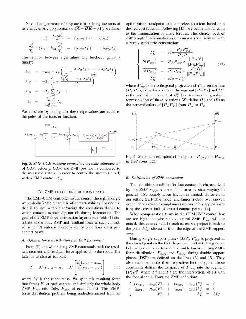
optimization standpoint, one can select solutions based on adesired cost function. Following [15], we define this functionas the minimization of ankle torques. This choice togetherwith simple approximations yields an analytical solution witha purely geometric construction:

F czL = Mg

‖PRPoZMP‖

‖PRPL‖−−−−−→NP ZMPL =

−−−−−→PRP ZMP ×

‖PRN‖‖PRP

oZMP‖

−−−−−→NP ZMPR =

−−−−−→PLP ZMP ×

‖PLN‖‖PRP

oZMP‖

F czR = Mg − F cz

L

(12)

where P oZMP is the orthogonal projection of P ZMP on the line

(PRPL), N is the middle of the segment [PRPL] and F czi

is the vertical component of F ci . Fig. 4 shows the graphical

representation of these equations. We define (L) and (R) asthe perpendiculars of [PLPR] from PL to PR.

P L P RN

P ZMP

(L ) (R)

P oZMP

P ZMPL

P ZMPR

Fig. 4: Graphical description of the optimal P ZMPL and P ZMPR

in DSP from (12).

B. Satisfaction of ZMP constraints

The non-tilting condition for foot contacts is characterizedby the ZMP support area. This area is state-varying ingeneral [16], notably when friction is limited. However, inour setting (cart-table model and larger friction over unevenground thanks to sole compliance) we can safely approximateit by the convex hull of ground contact points [14].

When compensation terms in the COM-ZMP control laware too high, the whole-body control ZMP P c

ZMP will lieoutside this convex hull. In such cases, we project it back tothe point P s

ZMP closest to it on the edge of the ZMP supportarea.

During single support phases (SSP), P cZMP is projected at

the closest point on the foot shape in contact with the ground.Following our choice to minimize ankle torques during ZMP-force distribution, P ZMPL and P ZMPR during double supportphases (DSP) are defined on the lines (L) and (R). Theyalso must be inside their respective foot polygon. Thoseconstraints delimit the existence of P ZMPi into the segment[P 1

iP2i ] where P 1

i and P 2i are the intersections of (i) with

the foot shape i. From the ZMP definition: (xZMPR − xZMP)FzR + (xZMPL − xZMP)F

zL = 0

(yZMPR − yZMP)FzR + (yZMPL − yZMP)F

zL = 0

F zR + F z

L = Mg

which constraint the alignment of P ZMP, P ZMPL and P ZMPR .Hence, a reduced convex hull can be defined during DSP toconstraint P c

ZMP. The latter is defined by the convex polygondelimited by (P 1

RP2RP

2LP

1L), as depicted in Figure 5.

In the event where P cZMP lies between (L) and (R), we

choose to project it at the closest point on the reduced convexhull to keep the maximum dynamic on the COM. For P c

ZMP

outside (L) and (R), we use the same projection as in a SSPcase.

P L

P R

N

P cZMP

(L )

(R)

P 1L

P 1R

P 2L

P 2R

P sZMP

P oZMP

Fig. 5: Convex hull of ground contact points (dashed red) andreduced ZMP support area (black) in double support phaseswhen ZMP-force distribution minimizes ankle torques. Thecontrol ZMP P c

ZMP is projected to P sZMP.

V. FLOOR REACTION FORCE CONTROL LAYER

For humanoid robots that are controlled in position, forcedistribution control at the feet is realized by admittancecontrol [9]. The output from an admittance controller consistsof foot orientations and relative positions, whereas its intputis given by the resultant forces and CoPs computed by theZMP-force distributor. Let us define:

δi =

[P i

Θi

], µi =

F i

xCoPi

yCoPi

ΓzCoPi

(13)

Our model of the sole stiffness is given by:

µi = J i(µi)δi (14)

where the stiffness matrix J(µi) is obtained by linearizatonof a finite element model (FEM) of the soft sole at µi, asdetailed in [8]. Equation (14) is a nonlinear model of thesole contact state that we approximate around a nominal µ0

i

state. However, we noticed in experiments that the rotationalstiffness highly depends on the vertical force F z

i . We thenchose to model this dependance with the follwing model:

J i(Fzi ) = J i(µ

0i )

[I (0)

(0) kf (F zi )I

](15)

with kf (F zi ) = F z

i /Fz0i and I the identity matrix. Feedback

control of such a system is equivalent to a damping:

δi = D−1i (µci − µi) (16)

We thus obtain the following closed-loop error transferfunction:

∆µi = −J(F zi )D−1i ∆µi (17)

We choose the poles as λaI , so that D−1i = λaJ i(Fzi )−1.

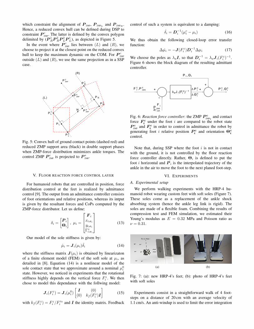
Figure 6 shows the block diagram of the resulting admittantcontroller.

λaJ i (F zi )− 1

F ci , P

cZMPi +

F iP ZMPizΓ CoPi

−

∆ P ci

∆ Θ ci

+

P i ,Θ i

+P ci ,Θ

ci

Fig. 6: Reaction force controller: the ZMP P cZMPi

and contactforce F c

i under the foot i are compared to the robot stateP c

ZMPand F c

i in order to control in admittance the robot bygenerating foot i relative position P c

i and orientation Θci

control.

Note that, during SSP where the foot i is not in contactwith the ground, it is not controlled by the floor reactionforce controller directly. Rather, Θi is defined to put thefoot i horizontal and P i is the interpolated trajectory of theankle in the air to move the foot to the next planed foot-step.

VI. EXPERIMENTS

A. Experimental setup

We perform walking experiments with the HRP-4 hu-manoid robot wearing custom feet with soft soles (Figure 7).These soles come as a replacement of the ankle shockabsorbing system (hence the ankle leg link is rigid). Thesoles are made of a flexible foam. Combining the results ofcompression test and FEM simulation, we estimated theirYoung’s modulus as E = 0.32 MPa and Poisson ratio asν = 0.31.

(a) (b)

Fig. 7: (a): new HRP-4’s feet; (b): photo of HRP-4’s feetwith soft soles

Experiments consist in a straightforward walk of 4 foot-steps on a distance of 20 cm with an average velocity of1.1 cm/s. An anti-windup is used to limit the error integration

by defining a sliding integration windows of 400 ms. The SSPand DSP durations given to the WPG are respectively set at1 s and 2 s. No ground information is given preliminary forwalking, i.e. the whole experiment is terrain-blind.

The poles of the ZMP-COM tracking controller are set to(−4,−4,−3,−ωc) while Tp = 0.11 s. In order to minimizerobot vibrations, kf is saturated between [0.5 − 1.5] duringDSP and at 0.9 during SSP. HRP-4’s low-level controlfrequency being 200 Hz, we choose λa = −200 Hz. The

nominal µ0i states are set to F 0

i = [0 0Mg

2]T , P 0

CoPi= P i

and Γz0CoPi = 0.

We used a simple COM state observer based on jointencoders, the assumption that contacts do not translate, andan estimate of the pelvis orientation frame provided bythe robot software. This simple observer results in littlemismatch between measures and actual COM location: instatic equilibrium, projected COM and ZMP locations differby roughly 2 cm. Nonetheless, our closed-loop controllerrecovers from this static error and achieves walking withsoft soles.

B. Walking on flat floor and gravel

Without a deformation estimator, HRP-4 was unable towalk on gravel without and with soft soles. With an offlinedeformation estimator, the robot manages to walk on flatground but not on gravel. Furthermore, it then deals with avery limited range of perturbations/uncertainties.

With our closed-loop controller, the robot succeeded inwalking on flat ground and on a bed of gravel with agranularity of 10/20 mm. Figure 8 shows measurements forwalking over gravel. These being similar to those observedover flat floor, to the exception of an increase in amplitudeon ZMP-COM oscillations, the discussion will now focus onthe earliest.

Figure 8a and 8b represent the ZMP and COM in thedirection of respectively x- and y-axes controlled by theZMP-COM control layer. The ZMP also remains withinthe support area. Some oscillations on the COM, and byextension the ZMP that controls it, are visible. They aremostly due to gravel irregularities and abrupt changes incontact surface during landing phases. The action of the ZMPcontrol P c

ZMP is clearly visible in the controlled movement ofZMP in order to keep the COM close to its reference.

Figure 8c represents the vertical ground reaction forces(GRF) controlled by the admittance of the reaction forcecontroller. The measure corresponds to the control withirregularities during transition between DSP and SSP whenone foot takes off and lands on the ground. Some impactsare visible at landing and are quickly absorbed by the soleand the admittance controller. These observations validate thedesign of our deformation estimator model and floor reactionforce controller.

Figures 8d, 8e and 8f represent the CoP under each foot,both controlled by the floor reaction control layer. Overall,measurements track well the references. As for the GRF,peaks of ZMP and CoP under the left foot appear due to

an early landing foot. Oscillations in CoP and ZMP controlsresult from a combination of (1) gravel irregularities and (2)significant noise in COM velocity estimation. This noise iswell distributed and with the mechanical lag, these vibrationsare absorbed and have low impact on the actual measuredZMP.

The accompanying video shows experiments on the realrobot: eight steps walking fully on gravel, as well as with atransition from wooden plank ground to gravel (Figure 1).

VII. CONCLUSION

In this paper, we designed a closed-loop controller basedon linear inverted pendulum tracking and an admittancecontrol of ground reaction forces combined with a simpledeformation estimator. We achieved walking with HRP-4 onflat and gravel grounds.

Robot stabilization depends on the identification of themechanical lag time constant Tp of ZMP response and theadaptation of the WPG to this time constant to choosethe phase duration. Up to now, the WPG used for ourexperiments generates motion trajectories offline. We thenplan to improve biped locomotion by using an adaptiveonline WPG (in terms of foot impact detection) coupled withan online estimation of the lags time constant and to changethe phase durations in order to better stabilize the robot whenthe ground properties are changing. We will also test walkingon other irregular terrains and larger steps.

In this paper, we added a thick squared soft sole undereach foot of a humanoid robot. In the near future, we willtest the developed controller on a robot with the optimizedsoles designed in [17].

REFERENCES

[1] K. Hirai, M. Hirose, Y. Haikawa, and T. Takenaka, “The developmentof honda humanoid robot,” in IEEE International Conference onRobotics and Automation, vol. 2. Leuven, Belgium: IEEE, May 1998,pp. 1321–1326.

[2] K. Kaneko, F. Kanehiro, S. Kajita, H. Hirukawa, T. Kawasaki, M. Hi-rata, K. Akachi, and T. Isozumi, “Humanoid robot hrp-2,” in IEEEInternational Conference on Robotics and Automation, New Orleans,USA, April 2004, pp. 1083–1090.

[3] O. Bruneau, F. B. Ouezdou, and J.-G. Fontaine, “Dynamic walkof a bipedal robot having flexible feet,” in IEEE/RSJ InternationalConference on Intelligent Robots and Systems, vol. 1. Maui, USA:IEEE, 29 October 2001, pp. 512–517.

[4] J. Vaillant, A. Kheddar, H. Audren, F. Keith, S. Brossette, A. Escande,K. Bouyarmane, K. Kaneko, M. Morisawa, P. Gergondet, E. Yoshida,S. Kajita, and F. Kanehiro, “Multi-contact vertical ladder climbing withan hrp-2 humanoid,” Autonomous Robots, vol. 40, no. 3, pp. 561–580,2016.

[5] J. Yamaguchi and A. Takanishi, “Multisensor foot mechanism withshock absorbing material for dynamic biped walking adapting tounknown uneven surfaces,” in IEEE International Conference on Mul-tisensor Fusion and Integration for Intelligent systems, WashingtonDC, USA, December 1996, pp. 233–240.

[6] G. De Magistris, A. Pajon, S. Miossec, and A. Kheddar, “Humanoidwalking with compliant soles using a deformation estimator,” in Inter-national Conference on Robotics and Automation (ICRA), Stockholm,Sweden, 2016.

[7] A. Pajon, G. De Magistris, S. Miossec, K. Kaneko, and A. Kheddar,“A humanoid walking pattern generator for sole design optimization,”in International Conference on Advanced Robotics (ICAR), Istanbul,Turkey, 2015.

0 5 10 15 20 25−0.1

−0.05

0

0.05

0.1

0.15

0.2

0.25

0.3

0.35x(t)iofiZMPiandiCOM

t[s]

x[m

]

ZMPirefCOMirefZMPicontrolZMPimesCOMimesanklesipositionfooticontactiarea

(a)

0 5 10 15 20 25−0.2

−0.15

−0.1

−0.05

0

0.05

0.1

0.15

0.2y(t) of ZMP and COM

t[s]

y[m

]

ZMP refCOM ref

ZMP control

ZMP mes

COM mes

ankles positionfoot contact area

(b)

0 5 10 15 20 25−100

0

100

200

300

400

500

600Vertical ground reaction force under each foot

t[s]

F[N

]

Right foot controlLeft foot controlRight foot mesLeft foot mes

(c)

0 5 10 15 20 25−0.1

−0.05

0

0.05

0.1

0.15

0.2

0.25

0.3

0.35x(t)loflCoPlunderlrightlfoot

t[s]

x[m

]

ZMPlrefCOMlrefCoPlrightlcontrolCoPlrightlmesankleslpositionfootlcontactlarea

(d)

0 5 10 15 20 25−0.1

−0.05

0

0.05

0.1

0.15

0.2

0.25

0.3

0.35x(t)pofpCoPpunderpleftpfoot

t[s]

x[m

]

ZMPprefCOMprefCoPpleftpcontrolCoPpleftpmesanklesppositionfootpcontactparea

(e)

0 5 10 15 20 25−0.2

−0.15

−0.1

−0.05

0

0.05

0.1

0.15

0.2y(t)loflCoPlunderleachlfoot

t[s]

y[m

]

ZMPlrefCOMlrefZMPlmesCoPlrightlcontrolCoPlleftlcontrolCoPlrightlmesCoPlleftlmesankleslpositionfootlcontactlarea

(f)

Fig. 8: Walking over gravel (granulometry: 10/20 mm): (a,b) ZMP and COM, (c) Vertical ground reaction forces and (d,e,f)CoP under each foot: measured compared with the references along x/y axes during a four steps and 20cm long.

[8] G. De Magistris, A. Pajon, S. Miossec, and A. Kheddar, “Optimizedhumanoid walking with soft soles,” Robotics and Autonomous Systems,vol. 95, pp. 52–63, 2017.

[9] J. De Schutter, H. Bruyninckx, W.-H. Zhu, and M. Spong, “Force con-trol: a bird’s eye view,” Control Problems in Robotics and Automation,pp. 1–17, 1998.

[10] K. Bouyarmane, J. Vaillant, F. Keith, and A. Kheddar, “Exploringhumanoid robots locomotion capabilities in virtual disaster responsescenarios,” in IEEE-RAS International Conference on HumanoidRobots, Osaka, 2012.

[11] T. Sugihara, “Standing stabilizability and stepping maneuver in planarbipedalism based on the best com-zmp regulator,” in Robotics and Au-tomation, 2009. ICRA’09. IEEE International Conference on. IEEE,2009, pp. 1966–1971.

[12] S. Kajita, M. Morisawa, K. Miura, S. Nakaoka, K. Harada, K. Kaneko,F. Kanehiro, and K. Yokoi, “Biped walking stabilization based onlinear inverted pendulum tracking,” in IEEE/RSJ International Con-ference on Intelligent Robots and Systems, Taipei, Taiwan, October 18- 22 2010, pp. 4489–4496.

[13] M. Morisawa, S. Kajita, F. Kanehiro, K. Kaneko, K. Miura, andK. Yokoi, “Balance control based on capture point error compensationfor biped walking on uneven terrain,” in Humanoid Robots (Hu-manoids), 2012 12th IEEE-RAS International Conference on. IEEE,2012, pp. 734–740.

[14] S. Kajita and B. Espiau, Handbook of Robotics. Springer-Verlag,2008, ch. Legged Robots, pp. 361–389.

[15] P. M. Wensing, G. Bin Hammam, B. Dariush, and D. E. Orin,“Optimizing foot centers of pressure through force distribution ina humanoid robot,” International Journal of Humanoid Robotics,vol. 10, no. 03, p. 1350027, 2013.

[16] S. Caron, Q.-C. Pham, and Y. Nakamura, “Zmp support areas formulticontact mobility under frictional constraints,” IEEE Transactionson Robotics, vol. 33, no. 1, pp. 67–80, 2017.

[17] G. De Magistris, S. Miossec, A. Escande, and A. Kheddar, “Design ofoptimized soft soles for humanoid robots,” Robotics and AutonomousSystems, vol. 95, pp. 129 – 142, 2017.