arX

iv:h

ep-t

h/96

0617

1 v4

16

Oct

199

7

On the Existence of Undistorted Progressive Waves(UPWs) of Arbitrary Speeds 0 ≤ v <∞ in Nature

Waldyr A. Rodrigues, Jr.(a) and Jian-Yu Lu(b)

(a) Instituto de Matematica, Estatıstica e Computacao CientıficaIMECC-UNICAMP; CP 6065, 13081-970, Campinas, SP, Brasile-mail: walrod@ime.unicamp.br

(b) Biodynamics Research Unit, Department of Physiology and BiophysicsMayo Clinic and Foundation, Rochester, MN55905, USAe-mail: jian@us0.mayo.edu

Abstract

We present the theory, the experimental evidence and fundamental phys-ical consequences concerning the existence of families of undistorted progres-sive waves (UPWs) of arbitrary speeds 0 ≤ v < ∞, which are solutions ofthe homogeneous wave equation, Maxwell equations, Dirac, Weyl and Klein-Gordon equations.

PACS numbers: 41.10.Hv; 03.30.+p; 03.40Kf

1. Introduction

In this paper we present the theory, the experimental evidence, and the fun-damental physical consequences concerning the existence of families of undistortedprogressive waves (UPWs)(∗) moving with arbitrary speeds(∗∗) 0 ≤ v <∞. We showthat the main equations of theoretical physics, namely: the scalar homogeneouswave equation (HWE); the Klein-Gordon equation (KGE); the Maxwell equations,the Dirac and Weyl equations have UPWs solutions in a homogeneous medium, in-cluding the vacuum. By UPW, following Courant and Hilbert[1] we mean that theUPW waves are distortion free, i.e. they are translationally invariant and thus donot spread, or they reconstruct their original form after a certain period of time.Explicit examples of how to construct the UPWs solutions for the HWE are found inAppendix A. The UPWs solutions to any field equations have infinite energy. How-ever, using the finite aperture approximation (FAA) for diffraction (Appendix A),

(∗)UPW is used for the singular, i.e., for undistorted progressive wave.(∗∗)We use units where c = 1, c being the so called velocity of light in vacuum.

1

we can project quasi undistorted progressive waves (QUPWs) for any field equationwhich have finite energy and can then in principle be launched in physical space.

In section 2 we show results of a recent experiment proposed and realized byus where the measurement of the speeds of a FAA to a subluminal(∗) Bessel pulse[eq.(2.1)] and of the FAA to a superluminal X-wave [eq.(2.5)] are done. The resultsare in excellent agreement with the theory.

In section 3 we discuss some examples of UPWs solutions of Maxwell equa-tions; (i) subluminal solutions which are interesting concerning some recent attemptsappearing in the literature[2,3,4] of construction of purely electromagnetic particles(PEP) and (ii) a superluminal UPW solution of Maxwell equations called the su-perluminal electromagnetic X-wave[5] (SEXW). We briefly discuss how to launch aFAA to SEXW. In view of the experimental results presented in section 2 we areconfident that such electromagnetic waves will be produced in the next few years. Insection 4 we discuss the important question concerning the speed of propagation ofthe energy carried by superluminal UPWs solutions of Maxwell equations, clearingsome misconceptions found in the literature. In section 5 we show that the experi-mental production of a superluminal electromagnetic wave implies in a breakdownof the Principle of Relativity. In section 6 we present our conclusions.

Appendix B presents a unified theory of how to construct UPWs of arbitraryspeeds 0 ≤ v < ∞ which are solutions of Maxwell, Dirac and Weyl equations. Ourunified theory is based on the Clifford bundle formalism[6,7,8,9,10] where all fieldsquoted above are represented by objects of the same mathematical nature. We takethe care of translating all results in the standard mathematical formalisms used byphysicists in order for our work to be usefull for a larger audience.

Before starting the technical discussions it is worth to briefly recall the history ofthe UPWs of arbitrary speeds 0 ≤ v <∞, which are solutions of the main equationsof theoretical physics.

To the best of our knowledge H. Bateman[11] in 1913 was the first person topresent a subluminal UPW solution of the HWE. This solution corresponds to whatwe called the subluminal spherical Bessel beam in Appendix A [see eq.(A.31)]. Ap-parently this solution has been rediscovered and used in diverse contexts manytimes in the literature. It appears, e.g., in the papers of Mackinnon[12] of 1978 and ofGueret and Vigier[13] and more recently in the papers of Barut and collaborators[14,15].In particular in[14] Barut also shows that the HWE has superluminal solutions. In

(∗)In this experiment the waves are sound waves in water and, of course, the meaning of thewords subluminal, luminal and superluminal in this case is that the waves travel with speed less,equal or greater than cs, the so called velocity of sound in water.

2

1987 Durnin and collaborators rediscovered a subluminal UPW solution of the HWEin cylindrical coordinates[16,17,18]. These are the Bessel beams of section A4 [seeeq.(A.41)]. We said rediscovered because these solutions are known at least since1941, as they are explicitly written down in Stratton’s book[19]. The important pointhere is that Durnin[16] and collaborators constructed an optical subluminal Besselbeam. At that time they didn’t have the idea of measuring the speed of the beams,since they were interested in the fact that the FAA to these beams were quasi UPWsand could be very usefull for optical devices. Indeed they used the term “diffraction-free beams” which has been adopted by some other authors later. Other authorsstill use for UPWs the term non-dispersive beams. We quote also that Hsu andcollaborators[20] realized a FAA to the J0 Bessel beam [eq.(A.41)] with a narrow bandPZT ultrasonic transducer of non-uniform poling. Lu and Greenleaf[21] produced thefirst J0 nondiffracting annular array transducers with PZT ceramic/polymer com-posite and applied it to medical acoustic imaging and tissue characterization[22,23].Also Campbell et al[24] used an annular array to realize a FAA to a J0 Bessel beamand compared the J0 beam to the so called axicon beam [25]. For more on this topicsee[26].

Luminal solutions of a new kind for the HWE and Maxwell equations, alsoknown as focus wave mode [FWM] (see Appendix A), have been discovered byBrittingham [27] (1983) and his work inspired many interesting and important studiesas, e.g.,[29−40].

To our knowledge the first person to write about the possibility of a superluminalUPW solution of HWE and, more important, of Maxwell equations was Band[41,42].He constructed a superluminal electromagnetic UPW from the modified Bessel beam[eq.(A.42)] which was used to generate in an appropriate way an electromagneticpotential in the Lorentz gauge. He suggested that his solution could be used toeventually launch a superluminal wave in the exterior of a conductor with cylin-drical symmetry with appropriate charge density. We discuss more some of Band’sstatements in section 4.

In 1992 Lu and Greenleaf[43] presented the first superluminal UPW solutionof the HWE for acoustic waves which could be launched by a physical device[44].They discovered the so called X-waves, a name due to their shape (see Fig. 3).In the same year Donnelly and Ziolkowski[45] presented a thoughtfull method forgenerating UPWs solutions of homogeneous partial equations. In particular theystudied also UPW solutions for the wave equation in a lossy infinite medium and tothe KGE. They clearly stated also how to use these solutions to obtain through theHertz potential method (see appendix B, section B3) UPWs solutions of Maxwell

3

equations.In 1993 Donnely and Ziolkowski[46] reinterpreted their study of[45] and obtained

subluminal, luminal and superluminal UPWs solutions of the HWE and of the KGE.In Appendix A we make use of the methods of this important paper in order to obtainsome UPWs solutions. Also in 1992 Barut and Chandola[47] found superluminalUPWs solutions of the HWE. In 1995 Rodrigues and Vaz[48] discovered in quitean independent way(∗) subluminal and superluminal UPWs solutions of Maxwellequations and the Weyl equation. At that time Lu and Greenleaf[5] proposed alsoto launch a superluminal electromagnetic X-wave.(∗∗)

In September 1995 Professor Ziolkowski took knowledge of[48] and informed oneof the authors [WAR] of his publications and also of Lu’s contributions. Soon acollaboration with Lu started which produced this paper. To end this introductionwe must call to the reader’s attention that in the last few years several important ex-periments concerning the superluminal tunneling of electromagnetic waves appearedin the literature[51,52]. Particularly interesting is Nimtz’s paper[53] announcing thathe transmitted Mozart’s Symphony # 40 at 4.7c through a retangular waveguide.The solutions of Maxwell equations in a waveguide lead to solutions of Maxwellequations that propagate with subluminal or superluminal speeds. These solutionscan be obtained with the methods discussed in this paper and will be discussed inanother publication.

2. Experimental Determination of the Speeds of AcousticFinite Aperture Bessel Pulses and X-Waves.

In appendix A we show the existence of several UPWs solutions to the HWE,in particular the subluminal UPWs Bessel beams [eq.(A.36)] and the superluminalUPWs X-waves [eq.(A.52)]. Theoretically the UPWs X-waves, both the broad-bandand band limited [see eq.(2.4)] travel with speed v = cs/ cos η > 1. Since only FAAto these X-waves can be launched with appropriate devices, the question arises ifthese FAA X-waves travel also with speed greater than cs, what can be answeredonly by experiment. Here we present the results of measurements of the speeds of a

(∗)Rodrigues and Vaz are interested in obtaining solutions of Maxwell equations characterizedby non-null field invariants, since solutions of this kind are[49,50] necessary in proving a surprisingrelationship between Maxwell and Dirac equations.

(∗∗)A version of [5] was submitted to IEEE Trans. Antennas Propag. in 1991. See reference40 of[43].

4

FAA to a broad band Bessel beam, called a Bessel pulse (see below) and of a FAAto a band limited X-wave, both moving in water. We write the formulas for thesebeams inserting into the HWE the parameter cs known as the speed of sound inwater. In this way the dispersion relation [eq.(A.37)] must read

ω2

c2s− k2 = α2 . (2.1)

Then we write for the Bessel beams

Φ<Jn

(t, ~x) = Jn(αρ)ei(kz−ωt+nθ), n = 0, 1, 2, . . . (2.2)

Bessel pulses are obtained from eq.(2.2) by weighting it with a transmitting transferfunction, T (ω) and then linearly superposing the result over angular frequency ω,i.e., we have

Φ<JBBn

(t, ~x) = 2πeinθJn(αρ)F−1[T (ω)eikz], (2.3)

where F−1 is the inverse Fourier transform. The FAA to Φ<JBBn

will be denoted byFAAΦ<

JBBn(or Φ<

FAJn).

We recall that the X-waves are given by eq.(A.52), i.e.,

Φ>Xn

(t, ~x) = einθ∫ ∞

0B(k)Jn(kρ sin η)e−k[a0−i(z cos η−cst)]dk , (2.4)

where k = k/ cos η, k = ω/cs. By choosing B(k) = a0 we have the infinite aperturebroad bandwidth X-wave [eq.(A.53)] given by

Φ>XBBn

(t, ~x) =a0(ρ sin η)neinθ

√M(τ +

√M)n

,

(2.5)

M = (ρ sin η)2 + τ 2, τ = [a0 − i(z cos η − cst)].

A FAA to Φ>XBBn

will be denoted by FAAΦ>XBBn

. When B(k) in eq.(2.4) is differentfrom a constant, e.g., if B(k) is the Blackman window function we denote the X-wave by Φ>

XBLn, where BL means band limited. A FAA to Φ>

XBLnwill be denoted

FAAΦXBLn. Also when T (ω) in eq.(2.3) is the Blackman window function we denote

the respective wave by ΦJBLn.

As discussed in Appendix A and detailed in[26,44] to produce a FAA to a givenbeam the aperture of the transducer used must be finite. In this case the beamsproduced, in our case FAAΦJBL0

and FAAΦXBB0, have a finite depth of field[26]

5

(DF)(∗) and can be approximately produced by truncating the infinite aperturebeams ΦJBL0

and ΦXBB0(or ΦXBL0

) at the transducer surface (z = 0). Broad bandpulses for z > 0 can be obtained by first calculating the fields at all frequencies witheq.(A.28), i.e.,

˜ΦFA(ω, ~x) =

1

iλ

∫ a

0

∫ π

−πρ′dρ′dθ′

˜Φ(ω, ~x′)

eikR

R2z

(2.6)

+1

2π

∫ a

0

∫ π

−πρ′dρ′dθ′

˜Φ(ω, ~x′)

eikR

R3z,

where the aperture weighting function˜Φ(ω, ~x′) is obtained from the temporal Fourier

transform of eqs.(2.3) and (2.4). If the aperture is circular of radius a [as in eq.(2.6)],the depth of field of the FAAΦJBL0

pulse, denoted BZmax and the depth of field ofthe FAAΦXBB0

or FAA ΦXBL0denoted by XZmax are given by[26]

BZmax = a

√(ω0

csα

)2

− 1 ; XZmax = a cot η. (2.7)

For the FAAΦJBL0pulse we choose T (ω) as the Blackman window function[54]

that is peaked at the central frequency f0 = 2.5MHz with a relative bandwidth ofabout 81% (−6 dB bandwidth divided by the central frequency). We have

B(k) =

a0

[0.42 − 0.5

πk

k0

+ 0.08 cos2πk

k0

], 0 ≤ k ≤ 2k0;

0 otherwise.

(2.8)

The “scaling factor” in the experiment is α = 1202.45m−1 and the weighting function˜ΦJBB0

(ω, ~x) in eq.(2.6) is approximated with stepwise functions. Practically this isdone with the 10-element annular array transfer built by Lu and Greenleaf[26,44].The diameter of the array is 50mm. Fig. 1(∗∗) shows the block diagram for theproduction of FAA Φ>

XBL0and FAAΦ<

JBL0. The measurement of the speed of the

FAA Bessel pulse has been done by comparing the speed with which the peak of theFAA Bessel pulse travels with the speed of the peak of a pulse produced by a small

(∗)DF is the distance where the field maximum drops to half the value at the surface of thetransducer.

(∗∗)Reprinted with permission from fig. 2 of[44].

6

circular element of the array (about 4mm or 6.67λ in diameter, where λ is 0.6mmin water). This pulse travels with speed cs = 1.5mm/µs. The distance betweenthe peaks and the surface of the transducer are 104.33(9)mm and 103.70(5)mm forthe single-element wave and the Bessel pulse, respectively, at the same instant t ofmeasurement. The results can be seen in the pictures taken from of the experimentin Fig. 2. As predicted by the theory developed in Appendix A the speed of theBessel pulse is 0.611(3)% slower than the speed cs of the usual sound wave producedby the single element.

The measurement of the speed of the central peak of the FAA Φ>XBL0

waveobtained from eq.(2.4) with a Blackman window function [eq.(2.8)] has been done inthe same way as for the Bessel pulse. The FAAΦXBL0

wave has been produced bythe 10-element array transducer of 50mm of diameter with the techniques developedby Lu and Greenleaf[26,44]. The distances traveled at the same instant t by the singleelement wave and the X-wave are respectively 173.48(9)mm and 173.77(3)mm. Fig.3 shows the pictures taken from the experiment. In this experiment the axicon angleis η = 40. The theoretical speed of the infinite aperture X-wave is predicted to be0.2242% greater then cs. We found that the FAAΦXBB0

wave traveled with speed0.267(6)% greater then cs !

These results, which we believe are the first experimental determination of thespeeds of subluminal and superluminal quasi-UPWs FAAΦ>

JBL0and FAAΦ<

JBB0solu-

tions of the HWE, together with the fact that, as already quoted, Durnin[16] producedsubluminal optical Bessel beams, give us confidence that electromagnetic subluminaland superluminal waves may be physically launched with appropriate devices. Inthe next section we study in particular the superluminal electromagnetic X-wave(SEXW).

It is important to observe here the following crucial points: (i) The FAA ΦXBBnis

produced by the source (transducer) in a short period of time ∆t. However, differentparts of the transducer are activated at different times, from 0 to ∆t, calculated fromeqs.(A.9) and (A.28). As a result the wave is born as an integral object for time∆t and propagates with the same speed as the peak. This is exactly what has beenseen in the experiments and is corroborated by the computer simulations we did forthe superluminal electromagnetic waves (see section 3). (ii) One can find in almostall textbooks that the velocity of transport of energy for waves obeying the scalarwave equation (

1

c2∂2

∂t2−∇2

)φ = 0 (2.9)

7

is given by

~vε =~S

u, (2.10)

where ~S is the flux of momentum and u is the energy density, given by

~S = ∇φ∂φ∂t

, u =1

2

(∇φ)2 +

1

c2

(∂φ

∂t

)2 , (2.11)

from which it follows that

vε =|~S|u

≤ cs . (2.12)

Our acoustic experiment shows that for the X-waves the speed of transport ofenergy is cs/ cos η, since it is the energy of the wave that activates the detector(hydro-phone). This shows explicitly that the definition of vε is meaningless. Thisfundamental experimental result must be kept in mind when we discuss the meaningof the velocity of transport of electromagnetic waves in section 4.

Figure 1: Block diagram of acoustic production of Bessel pulse and X-Waves.

8

Figure 2: Propagation speed of the peak of Bessel pulse and its comparison with thatof a pulse produced by a small circular element (about 4 mm or 6.67 λ in diameter,where λ is 0.6 mm in water). The Bessel pulse was produced by a 50 mm diametertransducer. The distances between the peaks and the surface of the transducerare 104.339 mm and 103.705 mm for the single-element wave and the Bessel pulse,respectively. The time used by these pulses is the same. Therefore, the speed of thepeak of the Bessel pulse is 0.611(3)% slower than that of the single-element wave.

9

Figure 3: Propagation speed of peak of X-wave and its comparison with that ofa pulse produced by small circular element (about 4 mm or 6.67 λ, where λ is0.6 mm in water). The X-wave was produced by a 50 mm diameter transducer.The distance between the peaks and the surface of the transducer are 173.489 mmand 173.773 mm for the single-element wave and the X-wave, respectively. The timeused by these pulses is the same. Therefore, the speed of the peak of the X-waveis 0.2441(8)% faster than that of the single-element wave. The theoretical ratio for

X-waves and the speed of sound is(cs/ cos η − cs)

cs= 0.2442% for η = 4o.

10

3. Subluminal and Superluminal UPWs Solutions of MaxwellEquations(ME)

In this section we make full use of the Clifford bundle formalism (CBF) resumedin Appendix B, but we give translation of all the main results in the standard vec-tor formalism used by physicists. We start by reanalyzing in section 3.1 the planewave solutions (PWS) of ME with the CBF. We clarify some misconceptions and ex-plain the fundamental role of the duality operator γ5 and the meaning of i =

√−1 in

standard formulations of electromagnetic theory. Next in section 3.2 we discuss sub-luminal UPWs solutions of ME and an unexpected relation between these solutionsand the possible existence of purely electromagnetic particles (PEPs) envisaged byEinstein[55], Poincare[56], Ehrenfest[57] and recently discussed by Waite, Barut andZeni[2,3]. In section 3.3 we discuss in detail the theory of superluminal electromag-netic X-waves (SEXWs) and how to produce these waves by appropriate physicaldevices.

3.1 Plane Wave Solutions of Maxwell Equations

We recall that Maxwell equations in vacuum can be written as [eq.(B.6)]

∂F = 0, (3.1)

where F sec∧2(M) ⊂ sec Cℓ(M). The well known PWS of eq.(3.1) are obtained

as follows. We write in a given Lorentzian chart 〈xµ〉 of the maximal atlas of M(section B2) a PWS moving in the z-direction

F = feγ5kx , (3.2)

k = kµγµ, k1 = k2 = 0, x = xµγµ, (3.3)

where k, x ∈ sec∧1(M) ⊂ sec Cℓ(M) and where f is a constant 2-form. From

eqs.(3.1) and (3.2) we obtainkF = 0 (3.4)

Multiplying eq.(3.4) by k we getk2F = 0 (3.5)

and since k ∈ sec∧1(M) ⊂ sec Cℓ(M) then

k2 = 0 ↔ k0 = ±|~k| = ±k3, (3.6)

11

i.e., the propagation vector is light-like. Also

F 2 = F. F + F ∧ F = 0 (3.7)

as can be easily seen by multiplying both members of eq.(3.4) by F and taking intoaccount that k 6= 0. Eq(3.7) says that the field invariants are null.

It is interesting to understand the fundamental role of the volume element γ5

(duality operator) in electromagnetic theory. In particular since eγ5kx = cos kx +

γ5 sin kx, γ5 ≡ i, writing F = ~E + i ~B (see eq.(B.17)), f = ~e1 + i~e2, we see that

~E + i ~B = ~e1 cos kx− ~e2 sin kx+ i(~e1 sin kx+ ~e2 cos kx) . (3.8)

From this equation, using ∂F = 0, it follows that ~e1.~e2 = 0, ~k.~e1 = ~k.~e2 = 0 andthen

~E. ~B = 0 . (3.9)

This equation is important because it shows that we must take care with the i =√−1 that appears in usual formulations of Maxwell Theory using complex electric

and magnetic fields. The i =√−1 in many cases unfolds a secret that can only be

known through eq.(3.8). It also follows that ~k. ~E = ~k. ~B = 0, i.e., PWS of ME aretransverse waves. We can rewrite eq.(3.4) as

kγ0γ0Fγ0 = 0 (3.10)

and since kγ0 = k0 + ~k, γ0Fγ0 = −~E + i ~B we have

~kf = k0f. (3.11)

Now, we recall that in Cℓ+(M) (where, as we say in Appendix B, the typicalfiber is isomorphic to the Pauli algebra Cℓ3,0) we can introduce the operator of space

conjugation denoted by ∗ such that writing f = ~e+ i~b we have

f ∗ = −~e+ i~b ; k∗0 = k0 ; ~k∗ = −~k. (3.12)

We can now interpret the two solutions of k2 = 0, i.e. k0 = |~k| and k0 = −|~k| as

corresponding to the solutions k0f = ~kf and k0f∗ = −~kf ∗; f and f ∗ correspond

in quantum theory to “photons” of positive or negative helicities. We can interpretk0 = |~k| as a particle and k0 = −|~k| as an antiparticle.

Summarizing we have the following important facts concerning PWS of ME: (i)the propagation vector is light-like, k2 = 0; (ii) the field invariants are null, F 2 = 0;

12

(iii) the PWS are transverse waves, i.e., ~k. ~E = ~k. ~B = 0.

3.2 Subluminal Solutions of Maxwell Equations and Purely Electromag-netic Particles.

We take Φ ∈ sec(∧0(M)⊕∧4(M)) ⊂ sec Cℓ(M) and consider the following Hertz

potential π ∈ sec∧2(M) ⊂ sec Cℓ(M) [eq.(B.25)]

π = Φγ1γ2. (3.13)

We now writeΦ(t, ~x) = φ(~x)eγ5Ωt. (3.14)

Since π satisfies the wave equation, we have

∇2φ(~x) + Ω2φ(~x) = 0 . (3.15)

Solutions of eq.(3.15) (the Helmholtz equation) are well known. Here we considerthe simplest solution in spherical coordinates,

φ(~x) = Csin Ωr

r, r =

√x2 + y2 + z2, (3.16)

where C is an arbitrary real constant. From the results of Appendix B we obtainthe following stationary electromagnetic field, which is at rest in the reference frameZ where 〈xµ〉 are naturally adapted coordinates (section B2):

F0 =C

r3[sin Ωt(αΩr sin θ sinϕ− β sin θ cos θ cosϕ)γ0γ1

− sin Ωt(αΩr sin θ cosϕ+ β sin θ cos θ sinϕ)γ0γ2

+ sin Ωt(β sin2 θ − 2α)γ0γ3 + cos Ωt(β sin2 θ − 2α)γ1γ2 (3.17)

+ cos Ωt(β sin θ cos θ sinϕ+ αΩr sin θ cosϕ)γ1γ3

+ cos Ωt(−β sin θ cos θ cosϕ+ αΩr sin θ sinϕ)γ2γ3]

with α = Ωr cos Ωr− sin Ωr and β = 3α+Ω2r2 sin Ωr. Observe that F0 is regular atthe origin and vanishes at infinity. Let us rewrite the solution using the Pauli-algebrain Cℓ+(M). Writing (i ≡ γ5)

F0 = ~E0 + i ~B0 (3.18)

we get

13

~E0 = ~W sin Ωt, ~B0 = ~W cos Ωt, (3.19)

with

~W = −C(αΩy

r3− βxz

r5,−αΩx

r3− βyz

r5,β(x2 + y2)

r5− 2α

r3

). (3.20)

We verify that div ~W = 0, div ~E0 = div ~B0 = 0, rot ~E0+∂ ~B0/∂t = 0, rot ~B0−∂ ~E0/∂t =0, and

rot ~W = Ω ~W. (3.21)

Now, from eq.(B.88) we know that T0 =1

2F γ0F is the 1-form representing the

energy density and the Poynting vector. It follows that ~E0× ~B0 = 0, i.e., the solutionhas zero angular momentum. The energy density u = S00 is given by

u =1

r6[sin2 θ(Ω2r2α2 + β2 cos2 θ) + (β sin2 θ − 2α)2] (3.22)

Then∫ ∫ ∫

IR3 u dv = ∞. As explained in section A.6 a finite energy solution can beconstructed by considering “wave packets” with a distribution of intrinsic frequenciesF (Ω) satisfying appropriate conditions. Many possibilities exist, but they will notbe discussed here. Instead, we prefer to direct our attention to eq.(3.21). As itis well known, this is a very important equation (called the force free equation[2])that appears e.g. in hydrodynamics and in several different situations in plasmaphysics[58]. The following considerations are more important.

Einstein[55] among others (see[3] for a review) studied the possibility of construct-ing purely electromagnetic particles (PEPs). He started from Maxwell equations fora PEP configuration described by an electromagnetic field Fp and a current densityJp, where

∂Fp = Jp (3.23)

and rightly concluded that the condition for existence of PEPs is

Jp.Fp = 0. (3.24)

This condition implies in vector notation

ρp~Ep = 0, ~jp. ~Ep = 0, ~jp × ~Bp = 0. (3.25)

14

From eq.(3.24) Einstein concluded that the only possible solution of eq.(3.22) withthe subsidiary condition given by eq.(3.23) is Jp = 0. However, this conclusion iscorrect, as pointed in[2,3], only if J2

p > 0, i.e., if Jp is a time-like current density.However, if we suppose that Jp can be spacelike, i.e., J2

p < 0, there exists a referenceframe where ρp = 0 and a possible solution of eq.(3.24) is

ρp = 0, ~Ep. ~Bp = 0, ~jp = KC ~Bp, (3.26)

where K = ±1 is called the chirality of the solution and C is a real constant. In[2,3]

static solutions of eqs.(3.22) and (3.23) are exhibited where ~Ep = 0. In this case we

can verify that ~Bp satisfies

∇× ~Bp = KC ~Bp. (3.27)

Now, if we choose F0 ∈ sec∧2(M) ⊂ sec Cℓ(M) such that

F0 = ~E0 + i ~B0,~E0 = ~Bp cos Ωt, ~B0 = ~Bp sin Ωt

(3.28)

and Ω = KC > 0, we immediately realize that

∂F0 = 0. (3.29)

This is an amazing result, since it means that the free Maxwell equations mayhave stationary solutions that may be used to model PEPs. In such solutions thestructure of the field F0 is such that we can write

F0 = F′

p + F = i ~W cos Ωt− ~W sin Ωt,∂F

′

p = −∂F = J′

p,(3.30)

i.e., ∂F0 = 0 is equivalent to a field plus a current. This fact opens several interestingpossibilities for modeling PEPs (see also[4]) and we discuss more this issue in anotherpublication.

We observe that moving subluminal solutions of ME can be easily obtainedchoosing as Hertz potential, e.g.,

π<(t, ~x) = Csin Ωξ<ξ<

exp[γ5(ω<t− k<z)]γ1γ2, (3.31)

ω2< − k2

< = Ω2<;

ξ< = [x2 + y2 + γ2<(z − v<t)

2], (3.32)

γ< =1

√1 − v2

<

, v< = dω</dk<.

15

We are not going to write explicitly the expression for F< corresponding to π<

because it is very long and will not be used in what follows.We end this section with the following observations: (i) In general for sublu-

minal solutions of ME (SSME) the propagation vector satisfies an equation likeeq.(3.30). (ii) As can be easily verified, for a SSME the field invariants are non-null. (iii) A SSME is not a transverse wave. This can be seen explicitly fromeq.(3.21). Conditions (i), (ii) and (iii) are in contrast with the case of the PWS ofME. In[49,50] Rodrigues and Vaz showed that for free electromagnetic fields (∂F = 0)such that F 2 6= 0, there exists a Dirac-Hestenes equation (see section A.8) forψ ∈ sec(

∧0(M) +∧2(M) +

∧4(M)) ⊂ sec Cℓ(M) where F = ψγ1γ2ψ. This was thereason why Rodrigues and Vaz discovered subluminal and superluminal solutions ofMaxwell equations (and also of Weyl equation)[48] which solve the Dirac-Hestenesequation [eq.(B.40)].

3.3 The Superluminal Electromagnetic X-Wave (SEXW)

To simplify the matter in what follows we now suppose that the functions ΦXn

[eq.(A.52)] and ΦXBBn[eq.(A.53)] which are superluminal solutions of the scalar

wave equation are 0-forms sections of the complexified Clifford bundle CℓC(M) =IC ⊗ Cℓ(M) (see section B4). We rewrite eqs.(A.52) and (A.53) as(∗)

ΦXn(t, ~x) = einθ

∫ ∞

0B(k)Jn(kρ sin η)e−k[a0−i(z cos η−t)]dk (3.33)

and choosing B(k) = a0, we have

ΦXBBn(t, ~x) =

a0(ρ sin η)neinθ

√M(τ +

√M)n

(3.34)

M = (ρ sin η)2 + τ 2; τ = [a0 − i(z cos η − t)]. (3.35)

As in section 2, when a finite broadband X-wave is obtained from eq.(3.31) withB(k) given by the Blackman spectral function [eq.(2.8)] we denote the resulting X-wave by ΦXBLn

(BL means band limited wave). The finite aperture approximation(FAA) obtained with eq.(A.28) to ΦXBLn

will be denoted FAAΦXBLnand the FAA

to ΦXBBnwill be denoted by FAAΦXBBn

. We use the same nomenclature for theelectromagnetic fields derived from these functions. Further, we suppose now that

(∗)In what follows n = 0, 1, 2, . . .

16

the Hertz potential π, the vector potential A and the corresponding electromagneticfield F are appropriate sections of CℓC(M). We take

π = Φγ1γ2 ∈ sec IC ⊗ ∧2(M) ⊂ sec CℓC(M), (3.36)

where Φ can be ΦXn,ΦXBBn

,ΦXBLn, FAA ΦXBBn

or FAAΦXBLn. Let us start by

giving the explicit form of the FXBBn, i.e., the SEXWs. In this case eq.(B.81) gives

π = ~πm and~πm = ΦXBBn

z (3.37)

where z is the versor of the z-axis. Also, let ρ, θ be respectively the versors of theρ and θ directions where (ρ, θ, z) are the usual cylindrical coordinates. Writing

FXBBn= ~EXBBn

+ γ5~BXBBn

(3.38)

we obtain from equations (A.53) and (B.25):

~EXBBn= −ρ

ρ

∂2

∂t∂θΦXBBn

+ θ∂2

∂t∂ρΦXBBn

; (3.39)

~BXBBn= ρ

∂2

∂ρ∂zΦXBBn

+ θ1

ρ

∂2

∂θ∂zΦXBBn

+ z

(∂2

∂z2ΦXBBn

− ∂2

∂t2ΦXBBn

); (3.40)

Explicitly we get for the components in cylindrical coordinates:

( ~EXBBn)ρ = −1

ρnM3√M

ΦXBBn; (3.41a)

( ~EXBBn)θ =

1

ρi

M6√MM2

ΦXBBn; (3.41b)

( ~BXBBn)ρ = cos η( ~EXBBn

)θ; (3.41c)

( ~BXBBn)θ = − cos η( ~EXBBn

)ρ; (3.41d)

( ~BXBBn)z = − sin2 η

M7√M

ΦXBBn. (3.41e)

The functions Mi, (i = 2, . . . , 7) in (3.41) are:

M2 = τ +√M ; (3.42a)

M3 = n+1√Mτ ; (3.42b)

M4 = 2n+3√Mτ ; (3.42c)

17

M5 = τ + n√M ; (3.42d)

M6 = (ρ2 sin2 ηM4

M− nM3)M2 + nρ2M5

Msin2 η; (3.42e)

M7 = (n2 − 1)1√M

+ 3n1

Mτ + 3

1√M3

τ 2. (3.42f)

We immediately see from eqs.(3.41) that the FXBBnare indeed superluminal

UPWs solutions of ME, propagating with speed 1/ cos η in the z-direction. ThatFXBBn

are UPWs is trivial and that they propagate with speed c1 = 1/ cos η followsbecause FXBBn

depends only on the combination of variables (z − c1t) and anyderivatives of ΦXBBn

will keep the (z − c1t) dependence structure.

Now, the Poynting vector ~PXBBnand the energy density uXBBn

for FXBBnare

obtained by considering the real parts of ~EXBBnand ~BXBBn

. We have

(~PXBBn)ρ = −Re( ~EXBBn

)θRe( ~BXBBn)z; (3.43a)

(~PXBBn)θ = Re( ~EXBBn

)ρRe( ~BXBBn)z; (3.43b)

(~PXBBn)z = cos η

[|Re( ~EXBBn

)ρ|2 + |Re( ~EXBBn)θ|2

]; (3.43c)

uXBBn= (1 + cos2 η)

[|Re( ~EXBBn

)ρ|2 + |Re( ~EXBBn)θ|2

]+ |Re( ~BXBBn

)z|2.(3.44)

The total energy of FXBBnis then

εXBBn=∫ π

−πdθ∫ +∞

−∞dz∫ ∞

0ρ dρ uXBBn

(3.45)

Since as z → ∞, ~EXBBndecreases as 1/|z − t cos η|1/2, what occurs for the X-

branches of FXBBn, εXBBn

may not be finite. Nevertheless, as in the case of theacoustic X-waves discussed in section 2, we are quite sure that a FAAFXBLn

canbe launched over a large distance. Obviously in this case the total energy of theFAAFXBLn

is finite.We now restrict our attention to FXBB0

. In this case from eq.(3.40) and eqs.(3.43)

we see that ( ~EXBB0)ρ = ( ~BXBB0

)θ = (~PXBB0)θ = 0. In Fig. 4(∗) we see the

amplitudes of ReΦXBB0 [4(1)], Re( ~EXBB0

)θ [4(2)], Re( ~BXBB0)ρ [4(3)] and

Re( ~BXBB0)z [4(4)]. Fig. 5 shows respectively (~PXBB0

)ρ [5(1)], (~PXBB0)z [5(2)]

and uXBB0[5(3)]. The size of each panel in Figures 4 and 5 is 4m (ρ-direction) ×

(∗)Figures 4, 5 and 6 were reprinted with permission from[5].

18

2mm (z-direction) and the maxima and minima of the images in Figures 4 and 5(before scaling) are shown in Table 1, in MKSA units(∗∗).

ReΦXBB0 Re( ~EXBB0

)θ Re( ~BXBB0)ρ Re( ~BXBB0

)zmax 1.0 9.5 × 106 2.5 × 104 6.1min 0.0 −9.5 × 106 −2.5 × 104 −1.5

(~PXBB0)ρ (~PXBB0

)z UXBB0

max 2.4 × 107 2.4 × 1011 1.6 × 103

min −2.4 × 107 0.0 0.0

Table 1: Maxima and Minima of the zeroth-order nondiffracting

electromagnetic X waves (units: MKSA).

Fig. 6 shows the beam plots of FXBB0in Fig. 4 along one of the X-branches

(from left to right). Fig. 6(1) represents the beam plots of ReΦXBB0 (full line),

Re( ~EXBB0)θ (dotted line), Re( ~BXBB0

)ρ (dashed line) and Re( ~BXBB0)z (long

dashed line). Fig. 6(2) represents the beam plots of (~PXBB0)ρ (full line), (~PXBB0

)z

(dotted line) and uXBB0(dashed line).

3.4 Finite Aperture Approximation to FXBB0and FXBL0

From eqs.(3.40), (3.43) and (3.44) we see that ~EXBB0, ~BXBB0

, ~PXBB0and uXBB0

are related to the scalar field ΦXBB0. It follows that the depth of the field[5] (or non

diffracting distance — see section 2) of the FAAFXBB0and of the FAAFXBL0

, whichof course are to be produced by a finite aperture radiator, are equal and given by

Zmax = D/2 cot η, (3.46)

where D is the diameter of the radiator and η is the axicon angle. It can be provedalso[5] that for ΦXBL0

(and more generally for ΦXBLn), that Zmax is independent of

the central frequency of the spectrum B(k) in eq.(3.1). Then if we want, e.g., thatFXBB0

or FXBL0travel 115 km with a 20 m diameter radiator, we need η = 0.005o.

Figure 7 shows the envelope of ReFAAΦXBB0 obtained with the finite aperture

approximation (FAA) given by eq.(A.28), with D = 20 m, a0 = 0.05 mm andη = 0.005o, for distances z = 10 km [6(1)] and z = 100 km [6(2)], respectively,

(∗∗)Reprinted with permission from Table I of[5].

19

from the radiator which is located at the plane z = 0. Figures 7(3) and 7(4) showthe envelope of ReFAAΦXBL0

for the same distances and the same parameters(D, a0 and η) where B(k) is the following Blackman window function, peaked at thefrequency f0 = 700 GHz with a 6 dB bandwidth about 576 GHz:

B(k) =

a0[0.42 − 0.5 cos πk

k0

+ 0.08 cos 2πkk0

], 0 ≤ k ≤ 2k0;

0 otherwise;(3.47)

where k0 = 2πf0/c (c = 300, 000km/s). From eq.(3.46) it follows that for the abovechoice of D, a0 and η

Zmax = 115 km (3.48)

Figs. 8(1) and 8(2) show the lateral beam plots and Figs. 8(3) and 8(4) show theaxial beam plots respectively for ReFAAΦXBB0

and for ReFAAΦXBL0 used to

calculate FXBB0and FXBL0

. The full and dotted lines represent X-waves at distancesz = 10 km and z = 100 km. Fig. 9 shows the peak values of ReFAAΦXBB0

(full line) and ReFAAΦXBL0

(dotted line) along the z-axis from z = 3.45 km toz = 230 km. The dashed line represents the result of the exact ΦXBB0

solution. The6 dB lateral and axial beam widths of ΦXBB0

, which can be measured in Fig 7(1)and 7(2), are about 1.96 m and 0.17 mm respectively, and those of the FAAΦXBL0

are about 2.5 m and 0.48 mm as can be measured from 7(3) and 7(4). For ΦXBB0

we can calculate[43,26] the theoretical values of the 6 dB lateral (BWL) and axial(BWA) beam widths, which are given by

BWL =2√

3a0

| sin η| ; BWA =2√

3a0

| cos η| . (3.49)

With the values of D, a0 and η given above, we have BWL = 1.98 m and BWA =0.17 mm. These are to be compared with the values of these quantities for theFAAΦXBL0

.We remark also that eq.(3.46) says that Zmax does not depend on a0. Then we

can choose an arbitrarily small a0 to increase the localization (reduced BWL andBWA) of the X-wave without altering Zmax. Smaller a0 requires that the FAAΦXBL0

be transmitted with broader bandwidth. The depths of field of ΦXBB0and of ΦXBL0

that we can measure in Fig. 9 are approximately 109 km and 110 km, very close tothe value given by eq.(3.46) which is 115 km.

We conclude this section with the following observations.

(i) In general both subluminal and superluminal UPWs solutions of ME have nonnull field invariants and are not transverse waves. In particular our solutions

20

have a longitudinal component along the z-axis. This result is importantbecause it shows that, contrary to the speculations of Evans[59], we do notneed an electromagnetic theory with a non zero photon-mass, i.e., with Fsatisfying Proca equation in order to have an electromagnetic wave with alongitudinal component. Since Evans presents evidence[59] of the existence onlongitudinal magnetic fields in many different physical situations, we concludethat the theoretical and experimental study of subluminal and superluminalUPW solutions of ME must be continued.

(ii) We recall that in microwave and optics, as it is well known, the electromag-netic intensity is approximately represented by the magnitude of a scalar fieldsolution of the HWE. We already quoted in the introduction that Durnin[16]

produced an optical J0-beam, which as seen from eq.(3.1) is related to ΦXBB0

(ΦXBL0). If we take into account this fact together with the results of the

acoustic experiments described in section 2, we arrive at the conclusion thatsubluminal electromagnetic pulses J0 and also superluminal X-waves can belaunched with appropriate antennas using present technology.

(iii) If we take a look at the structure of e.g. the FAAΦXBB0[eq.(3.40)] plus

eq.(A.28) we see that it is a “packet” of wavelets, each one traveling withspeed c. Nevertheless, the electromagnetic X-wave wave that is an interfer-ence pattern is such that its peak travels with speed c/ cos η > 1. (Thisindeed happens in the acoustic experiment with c 7→ cs, see section 2). Sinceas discussed above we can project an experiment to launch the peak of theFAAΦXBB0

from a point z1 to a point z2, the question arises: Is the existenceof superluminal electromagnetic waves in conflict with Einstein’s Special Rel-ativity? We give our answer to this fundamental issue in section 5, but firstwe discuss in section 4 the speed of propagation of the energy associated witha superluminal electromagnetic wave.

21

Figure 4: Real part of field components of the exact solution superluminal electro-magnetic X-wave at distance z = ct/ cos η (η = 0.005o, a0 = 0.05 mm, n = 0).

22

Figure 5: Poynting flux and energy density of the exact solution superluminal elec-tromagnetic X-wave at distance z = ct/ cos η, (η = 0.005o, a0 = 0.05 mm, n = 0).

23

Figure 6: (6.1) Beam plots along the X-branches of FXBB0for ReΦXBB0

or Hertz

potential, Re( ~EXBB0)θ, Re( ~BXBB0

)ρ, and Re( ~BXBB0)z. (6.2) Beam plots for

(~PXBB0)ρ (full line), (~PXBB0

)z (dotted line) and uXBB0(dashed line).

24

Figure 7: 7(1) and 7(2) show the real part of FAAΦXBB0at distances z = 10 km

and z = 100 km from the radiator located at the plane z = 0 with D = 20 m andη = 0.005o. 7(3) and 7(4) show the real parts of FAAΦXBL0

for the same distances.

25

Figure 8: Beam plots of scalar X-waves (finite aperture).

26

Figure 9: Peak magnitude of X-waves along the z axis.

27

4. The Velocity of Transport of Energy of the UPWs Solu-tions of Maxwell Equations

Motivated by the fact that the acoustic experiment of section 2 shows that theenergy of the FAA X-wave travels with speed greater than cs and since we foundin this paper UPWs solutions of Maxwell equations with speeds 0 ≤ v < ∞, thefollowing question arises naturally: Which is the velocity of transport of the energyof a superluminal UPW (or quasi UPW) solution of ME?

We can find in many physics textbooks (e.g.[10]) and in scientific papers[41] thefollowing argument. Consider an arbitrary solution of ME in vacuum, ∂F = 0. Thenif F = ~E + i ~B (see eq.(B.17)) it follows that the Poynting vector and the energydensity of the field are

~P = ~E × ~B, u =1

2( ~E2 + ~B2). (4.1)

It is obvious that the following inequality always holds:

vε =|~P |u

≤ 1. (4.2)

Now, the conservation of energy-momentum reads, in integral form over a finitevolume V with boundary S = ∂V

∂

∂t

∫ ∫ ∫

Vdv

1

2( ~E2 + ~B2)

=∮

Sd~S. ~P (4.3)

Eq.(4.3) is interpreted saying that∮S d

~S. ~P is the field energy flux across the surface

S = ∂V , so that ~P is the flux density — the amount of field energy passing through aunit area of the surface in unit time. For plane wave solutions of Maxwell equations,

vε = 1 (4.4)

and this result gives origin to the “dogma” that free electromagnetic fields transportenergy at speed vε = c = 1.

However vε ≤ 1 is true even for subluminal and superluminal solutions of ME,as the ones discussed in section 3. The same is true for the superluminal modifiedBessel beam found by Band[41] in 1987. There he claims that since vε ≤ 1 there isno conflict between superluminal solutions of ME and Relativity Theory since whatRelativity forbids is the propagation of energy with speed greater than c.

28

Here we challenge this conclusion. The fact is that as is well known ~P is notuniquely defined. Eq(4.3) continues to hold true if we substitute ~P 7→ ~P + ~P ′ with

∇. ~P ′ = 0. But of course we can easily find for subluminal, luminal or superluminalsolutions of Maxwell equations a ~P ′ such that

|~P + ~P ′|u

≥ 1. (4.5)

We come to the conclusion that the question of the transport of energy in superlu-minal UPWs solutions of ME is an experimental question. For the acoustic superlu-minal X-solution of the HWE (see section 2) the energy around the peak area flowstogether with the wave, i.e., with speed c1 = cs/ cos η (although the “canonical”formula [eq.(2.10)] predicts that the energy flows with vε < cs). Since we can see nopossibility for the field energy of the superluminal electromagnetic wave to traveloutside the wave we are confident to state that the velocity of energy transport ofsuperluminal electromagnetic waves is superluminal.

Before ending we give another example to illustrate that eq.(4.2) (as is thecase of eq.(2.10)) is devoid of physical meaning. Consider a spherical conductor inelectrostatic equilibrium with uniform superficial charge density (total charge Q)and with a dipole magnetic moment. Then, we have

~E = Qr

r2; ~B =

C

r3(2 cos θ r + sin θ θ) (4.6)

and

~P = ~E × ~B =CQ

r5sin θϕ , u =

1

2

(Q2

r4+C2

r6(3 cos2 θ + 1)

). (4.7)

Thus|~P |u

=2CQr sin θ

r2Q2 + C2(3 cos2 θ + 1)6= 0 for r 6= 0. (4.8)

Since the fields are static the conservation law eq.(4.3) continues to hold true, asthere is no motion of charges and for any closed surface containing the sphericalconductor we have ∮

Sd~S. ~P = 0. (4.9)

But nothing is in motion! In view of these results we must investigate whetherthe existence of superluminal UPWs solutions of ME is compatible or not with thePrinciple of Relativity. We analyze this question in detail in the next section.

29

To end this section we recall that in section 2.19 of his book Stratton[19] presentsa discussion of the Poynting vector and energy transfer which essentially agrees withthe view presented above. Indeed he finished that section with the words: “By thisstandard there is every reason to retain the Poyinting-Heaviside viewpoint until aclash with new experimental evidence shall call for its revision.”(∗)

5. Superluminal Solutions of Maxwell Equations and thePrinciple of Relativity

In section 3 we showed that it seems possible with present technology to launchin free space superluminal electromagnetic waves (SEXWs). We show in the follow-ing that the physical existence of SEXWs implies a breakdown of the Principle ofRelativity (PR). Since this is a fundamental issue, with implications for all branchesof theoretical physics, we will examine the problem with great care. In section 5.1we give a rigorous mathematical definition of the PR and in section 5.2 we presentthe proof of the above statement.

5.1 Mathematical Formulation of the Principle of Relativity and ItsPhysical Meaning

In Appendix B we define Minkowski spacetime as the triple 〈M, g,D〉, whereM ≃ IR4, g is a Lorentzian metric and D is the Levi-Civita connection of g.

Consider now GM , the group of all diffeomorphisms of M , called the manifoldmapping group. Let T be a geometrical object defined in A ⊆ M . The diffeomor-phism h ∈ GM induces a deforming mapping h∗ : T 7→ h∗T = T such that:

(i) If f : M ⊇ A→ IR, then h∗f = f h−1 : h(A) → IR

(ii) If T ∈ sec T (r,s)(A) ⊂ sec T (M), where T (r,s)(A) is the sub-bundle of tensors oftype (r, s) of the tensor bundle T (M), then

(h∗T)he(h∗ω1, . . . , h∗ωr, h∗X1, . . . , h∗Xs) = Te(ω1, . . . , ωr, X1, . . . , Xs)

∀Xi ∈ TeA, i = 1, . . . , s, ∀ωj ∈ T ∗eA, j = 1, . . . , r, ∀e ∈ A.

(iii) If D is the Levi-Civita connection and X, Y ∈ sec TM , then

(h∗Dh∗Xh∗Y )heh∗f = (DXY )ef ∀e ∈M. (5.1)

(∗)Thanks are due to the referee for calling our attention to this point.

30

If fµ = ∂/∂xµ is a coordinate basis for TA and θµ = dxµ is the correspondingdual basis for T ∗A and if

T = T µ1...µr

ν1...νsθν1 ⊗ . . .⊗ θνs ⊗ fµ1

⊗ . . .⊗ fµr, (5.2)

thenh∗T = [T µ1...µr

ν1...νs h−1]h∗θ

ν1 ⊗ . . .⊗ h∗θνs ⊗ h∗fµ1

⊗ . . .⊗ h∗fµr. (5.3)

Suppose now that A and h(A) can be covered by the local chart (U, η) of the maximalatlas of M , and A ⊆ U, h(A) ⊆ U . Let 〈xµ〉 be the coordinate functions associatedwith (U, η). The mapping

x′µ = xµ h−1 : h(U) → IR (5.4)

defines a coordinate transformation 〈xµ〉 7→ 〈x′µ〉 if h(U) ⊇ A ∪ h(A). Indeed 〈x′µ〉are the coordinate functions associated with the local chart (V, ϕ) where h(U) ⊆ Vand U ∩ V 6= φ. Now, since it is well known that under the above conditionsh∗∂/∂x

µ ≡ ∂/∂x′µ and h∗dx

µ ≡ dx′µ, eqs.(5.3) and (5.4) imply that

(h∗T)〈x′µ〉(he) = T〈xµ〉(e), (5.5)

where T〈xµ〉(e) means the components of T in the chart 〈xµ〉 at the event e ∈ M ,i.e., T〈xµ〉(e) = T µ1...µr

ν1...νs(xµ(e)) and where T

′µ1...µrν1...νs

(x′µ(he)) are the components of

T = h∗T in the basis h∗∂/∂xµ = ∂/∂x′µ, h∗dxµ = dx

′µ, at the point h(e).Then eq.(5.6) reads

T′µ1...µr

ν1...νs(x

′µ(he)) = T µ1...µr

ν1...νs(xµ(e)), (5.6)

or using eq.(5.5)

T′µ1...µr

ν1...νs(x

′µ(e)) = (Λ−1)µ1

α1. . .Λβs

νsT

′α1...αr

β1...βs(x

′µ(h−1e)), (5.7)

where Λµα = ∂x

′µ/∂xα, etc.In appendix B we introduce the concept of inertial reference frames I ∈ sec TU ,

U ⊆M byg(I, I) = 1 and DI = 0. (5.8)

A general frame Z satisfies g(Z,Z) = 1, with DZ 6= 0. If α = g(Z, ) ∈ sec T ∗U , itholds

(Dα)e = ae ⊗ αe + σe + ωe +1

3θehe, e ∈ U ⊆ M, (5.9)

31

where a = g(A, ), A = DZZ is the acceleration and where ωe is the rotation tensor,σe is the shear tensor, θe is the expansion and he = g|He

where

TeM = [Ze] ⊕ [He]. (5.10)

He is the rest space of an instantaneous observer at e, i.e. the pair (e, Ze). Alsohe(X, Y ) = ge(pX, pY ), ∀X, Y ∈ TeM and p : TeM → He. (For the explicit formof ω, σ, θ, see[60]). From eqs.(5.9) and (5.10) we see that an inertial reference framehas no acceleration, no rotation, no shear and no expansion.

We introduce also in Appendix B the concept of a (nacs/I). A (nacs/I) 〈xµ〉 issaid to be in the Lorentz gauge if xµ, µ = 0, 1, 2, 3 are the usual Lorentz coordinatesand I = ∂/∂x0 ∈ sec TM . We recall that it is a theorem that putting I = e0 =∂/∂x0, there exist three other fields ei ∈ sec TM such that g(ei, ei) = −1, i = 1, 2, 3,and ei = ∂/∂xi.

Now, let 〈xµ〉 be Lorentz coordinate functions as above. We say that ℓ ∈ GM isa Lorentz mapping if and only if

x′µ(e) = Λµ

νxµ(e), (5.11)

where Λµν ∈ L↑+ is a Lorentz transformation. For abuse of notation we denote the

subset ℓ of GM such that eq.(5.12) holds true also by L↑+ ⊂ GM .When 〈xµ〉 are Lorentz coordinate functions, 〈x′µ〉 are also Lorentz coordinate

functions. In this case we denote

eµ = ∂/∂xµ, e′µ = ∂/∂x′µ, γµ = dxµ, γ′µ = dx

′µ ; (5.12)

when ℓ ∈ L↑+ ⊂ GM we say that ℓ∗T is the Lorentz deformed version of T.Let h ∈ GM . If for a geometrical object T we have

h∗T = T, (5.13)

then h is said to be a symmetry of T and the set of all h ∈ GM such that eq.(5.13)holds is said to be the symmetry group of T. We can immediately verify that forℓ ∈ L↑+ ⊂ GM

ℓ∗g = g, ℓ∗D = D, (5.14)

i.e., the special restricted orthochronous Lorentz group L↑+ is a symmetry group ofg and D.

In[62] we maintain that a physical theory τ is characterized by:

32

(i) the theory of a certain “species of structure” in the sense of Boubarki[63];

(ii) its physical interpretation;

(iii) its present meaning and present applications.

We recall that in the mathematical exposition of a given physical theory τ , thepostulates or basic axioms are presented as definitions. Such definitions mean thatthe physical phenomena described by τ behave in a certain way. Then, the definitionsrequire more motivation than the pure mathematical definitions. We call coordina-tive definitions the physical definitions, a term introduced by Reichenbach[64]. It isnecessary also to make clear that completely convincing and genuine motivations forthe coordinative definitions cannot be given, since they refer to nature as a wholeand to the physical theory as a whole.

The theoretical approach to physics behind (i), (ii) and (iii) above is then toadmit the mathematical concepts of the “species of structure” defining τ as prim-itives, and define coordinatively the observation entities from them. Reichenbachassumes that “physical knowledge is characterized by the fact that concepts are notonly defined by other concepts, but are also coordinated to real objects”. However,in our approach, each physical theory, when characterized as a species of structure,contains some implicit geometric objects, like some of the reference frame fields de-fined above, that cannot in general be coordinated to real objects. Indeed it wouldbe an absurd to suppose that all the infinity of IRF that exist in M must have amaterial support.

We define a spacetime theory as a theory of a species of structure such that, ifMod τ is the class of models of τ , then each Υ ∈ Mod τ contains a substructurecalled spacetime (ST). More precisely, we have

Υ = (ST,T1 . . .Tm , (5.15)

where ST can be a very general structure[62]. For what follows we suppose thatST = M = (M, g,D), i.e. that ST is Minkowski spacetime. The Ti, i = 1, . . . , mare (explicit) geometrical objects defined in U ⊆M characterizing the physical fieldsand particle trajectories that cannot be geometrized in Υ. Here, to be geometrizablemeans to be a metric field or a connection on M or objects derived from theseconcepts as, e.g., the Riemann tensor or the torsion tensor.

The reference frame fields will be called the implicit geometrical objects of τ ,since they are mathematical objects that do not necessarily correspond to propertiesof a physical system described by τ .

33

Now, with the Clifford bundle formalism we can formulate in Cℓ(M) all modernphysical theories (see Appendix B) including Einstein’s gravitational theory[6]. Weintroduce now the Lorentz-Maxwell electrodynamics (LME) in Cℓ(M) as a theoryof a species of structure. We say that LME has as model

ΥLME = 〈M, g,D, F, J, ϕi, mi, ei〉, (5.16)

where (M, g,D) is Minkowski spacetime, ϕi, mi, ei, i = 1, 2, . . . , N is the set ofall charged particles, mi and ei being the masses and charges of the particles andϕi : IR ⊃ I →M being the world lines of the particles characterized by the fact thatif ϕi∗ ∈ sec TM is the velocity vector, then ϕi = g(ϕi∗, ) ∈ sec Λ1(M) ⊂ sec Cℓ(M)and ϕi.ϕi = 1. F ∈ sec Λ2(M) ⊂ sec Cℓ(M) is the electromagnetic field and J ∈sec Λ1(M) ⊂ sec Cℓ(M) is the current density. The proper axioms of the theory are

∂F = JmiDϕi∗

ϕi = eiϕi · F (5.17)

From a mathematical point of view it is a trivial result that τLME has thefollowing property: If h ∈ GM and if eqs.(5.16) have a solution 〈F, J, (ϕi, mi, ei)〉 inU ⊆ M then 〈h∗F, h∗J, (h∗ϕi, mi, ei)〉 is also a solution of eqs.(5.16) in h(U). Sincethe result is true for any h ∈ GM it is true for ℓ ∈ L↑+ ⊂ GM , i.e., for any Lorentzmapping.

We must now make it clear that 〈F, J, ϕi, mi, ei〉 which is a solution of eq.(5.16)in U can be obtained only by imposing mathematical boundary conditions which wedenote by BU . The solution will be realizable in nature if and only if the mathe-matical boundary conditions can be physically realizable. This is indeed a nontrivialpoint[62] for in particular it says to us that even if 〈h∗F, h∗J, h∗ϕi, mi, ei〉 can be asolution of eqs.(5.16) with mathematical boundary conditions Bh(U), it may hap-pen that Bh(U) cannot be physically realizable in nature. The following statement,denoted PR1, is usually presented[62] as the Principle of (Special) Relativity in activeform:

PR1:Let ℓ ∈ L↑+ ⊂ GM . If for a physical theory τ and Υ ∈ Mod τ , Υ =〈M, g,D,T1, . . . ,Tm〉 is a possible physical phenomenon, then ℓ∗Υ = 〈M, g,D,l∗T1, . . . , l∗Tm〉 is also a possible physical phenomenon.

It is clear that hidden in PR1 is the assumption that the boundary conditionsthat determine ℓ∗Υ are physically realizable. Before we continue we introduce thestatement denoted PR2, known as the Principle of (Special) Relativity in passiveform[62]

34

PR2:“All inertial reference frames are physically equivalent or indistinguishable”.

We now give a precise mathematical meaning to the above statement.Let τ be a spacetime theory and let ST = 〈M, g,D〉 be a substructure of Mod τ

representing spacetime. Let I ∈ secTU and I ′ ∈ sec TV , U, V ⊆M , be two inertialreference frames. Let (U, η) and (V, ϕ) be two Lorentz charts of the maximal atlasof M that are naturally adapted respectively to I and I ′. If 〈xµ〉 and 〈x′µ〉 are thecoordinate functions associated with (U, η) and (V, ϕ), we have I = ∂/∂x0, I ′ =∂/∂x

′0.

Definition: Two inertial reference frames I and I ′ as above are said to be phys-ically equivalent according to τ if and only if the following conditions are satisfied:

(i) GM ⊃ L↑+ ∋ ℓ : U → ℓ(U) ⊆ V, x′µ = xµ ℓ−1 ⇒ I ′ = ℓ∗I

When Υ ∈ Modτ , Υ = 〈M, g,D,T1, . . .Tm〉, is such that g and D are definedover all M and Ti ∈ sec Cℓ(U) ⊂ sec Cℓ(M), calling o = 〈g,D,T1, . . .Tm〉, o solvesa set of differential equations in η(U) ⊂ IR4 with a given set of boundary conditionsdenoted bo〈x

µ〉, which we write as

Dα〈xµ〉(o〈xµ〉)e = 0 ; bo〈x

µ〉 ; e ∈ U (5.18)

and we must have:(ii) If Υ ∈ Mod τ ⇔ ℓ∗Υ ∈ Mod τ , then necessarily

ℓ∗Υ = 〈M, g,D, ℓ∗T1, . . . ℓ∗Tm〉 (5.19)

is defined in ℓ(U) ⊆ V and calling ℓ∗o ≡ g,D, ℓ∗T1, . . . , ℓ∗Tm we must have

Dα〈x

′µ〉(ℓ∗o〈x′µ〉)|ℓe = 0 ; bℓ∗o〈x′µ〉 ℓe ∈ ℓ(U) ⊆ V. (5.20)

In eqs.(5.18) and (5.20) Dα〈xµ〉 and Dα

〈x′µ〉mean α = 1, 2, . . . , m sets of differential

equations in IR4. The system of differential equations (5.19) must have the same

functional form as the system of differential equations (5.17) and bℓ∗o〈x′µ〉 must be

relative to 〈x′µ〉 the same as bo〈xµ〉 is relative to 〈xµ〉 and if bo〈x

µ〉 is physically realiz-

able then bℓ∗o〈x′µ〉 must also be physically realizable. We say under these conditions

that I ∼ I ′ and that ℓ∗o is the Lorentz deformed version of the phenomena describedby o.

Since in the above definition ℓ∗Υ = 〈M, g,D, ℓ∗T1, . . . , ℓ∗Tm〉, it follows thatwhen I ∼ I ′, then ℓ∗g = g, ℓ∗D = D (as we already know) and this means that the

35

spacetime structure does not give a preferred status to I or I ′ according to τ .

5.2 Proof that the Existence of SEXWs Implies a Breakdown of PR1

and PR2

We are now able to prove the statement presented at the beginning of this sec-tion, that the existence of SEXWs implies a breakdown of the Principle of Relativityin both its active (PR1) and passive (PR2) versions.

Let ℓ ∈ L↑+ ⊂ GM and let F , F ∈ sec Λ2(M) ⊂ sec Cℓ(M), F = ℓ∗F . Let F =ℓ∗F = RFR−1, where Fe = (1/2)Fµν(x

δ(ℓ−1e))γµγν and where R ∈ sec Spin+(1, 3) ⊂sec Cℓ(M) is a Lorentz mapping, such that γ

′µ = RγµR−1 = Λµαγ

α,Λµα ∈ L↑+ and let

〈xµ〉 and 〈x′µ〉 be Lorentz coordinate functions as before such that γµ = dxµ, γ′µ =

dx′µ and x

′µ = xµ ℓ−1. We write

Fe =1

2Fµν(x

δ(e))γµγν ; (5.22a)

Fe =1

2F ′µν(x

′δ(e))γ′µγ

′ν ; (5.22b)

F e =1

2F µν(x

δ(e))γµγν ; (5.23a)

F e =1

2F′µν(x

′δ(e))γ′µγ

′ν . (5.23b)

From (5.22a) and (5.22b) we get that

F ′αβ(x′δ(e)) = (Λ−1)µ

α(Λ−1)νβFµν(x

δ(e)). (5.24)

From (5.22a) and (5.23b) we also get

F αβ(xδ(e)) = ΛµαΛν

βFµν(xδ(ℓ−1e)) (5.25)

Now, suppose that F is a superluminal solution of Maxwell equation, in par-ticular a SEXW as discussed in section 3. Suppose that F has been producedin the inertial frame I with 〈xµ〉 as (nacs/I), with the physical device describedin section 3. F is generated in the plane z = 0 and is traveling with speedc1 = 1/ cos η in the negative z-direction. It will then travel to the future inspacetime, according to the observers in I. Now, there exists ℓ ∈ L↑+ such that

36

ℓ∗F = F = RFR−1 will be a solution of Maxwell equations and such that if thevelocity 1-form of F is vF = (c21 − 1)−1/2(1, 0, 0,−c1), then the velocity 1-form ofF is vF = (c

′21 − 1)−1/2(−1, 0, 0,−c′1), with c′1 > 1, i.e., vF is pointing to the past.

As its is well known F carries negative energy according to the observers in the Iframe.

We then arrive at the conclusion that to assume the validity of PR1 is to assumethe physical possibility of sending to the past waves carrying negative energy. Thisseems to the authors an impossible task, and the reason is that there do no existphysically realizable boundary conditions that would allow the observers in I tolaunch F in spacetime and such that it traveled to its own past.

We now show that there is also a breakdown of PR2, i.e., that it is not true thatall inertial frames are physically equivalent. Suppose we have two inertial frames Iand I ′ as above, i.e., I = ∂/∂x0, I ′ = ∂/∂x

′0.Suppose that F is a SEXW which can be launched in I with velocity 1-form as

above and suppose F is a SEXW built in I ′ at the plane z′ = 0 and with velocity1-form relative to 〈x′µ〉 given by vF = v

′µγ′µ and

vF =(

1√c21 − 1

, 0, 0,− c1√c21 − 1

)(5.26)

If F and F are related as above we see (See Fig.10) that F , which has positiveenergy and is traveling to the future according to I ′, can be sent to the past of theobservers at rest in the I frame. Obviously this is impossible and we conclude thatF is not a physically realizable phenomenon in nature. It cannot be realized in I ′

but F can be realized in I. It follows that PR2 does not hold.If the elements of the set of inertial reference frames are not equivalent then there

must exist a fundamental reference frame. Let I ∈ secTM be that fundamentalframe. If I ′ is moving with speed V relative to I, i.e.,

I ′ =1√

1 − V 2

∂

∂t− V√

1 − V 2∂/∂z , (5.27)

then, if observers in I ′ are equipped with a generator of SEXWs and if they preparetheir apparatus in order to send SEXWs with different velocity 1-forms in all pos-sible directions in spacetime, they will find a particular velocity 1-form in a givenspacetime direction in which the device stops working. A simple calculation yieldsthen, for the observes in I ′, the value of V !

In [65] Recami argued that the Principle of Relativity continues to hold true eventhough superluminal phenomena exist in nature. In this theory of tachyons there

37

exists, of course, a situation completely analogous to the one described above (calledthe Tolman-Regge paradox), and according to Recami’s view PR2 is valid becauseI ′ must interpret F a being an anti-SEXW carrying positive energy and going intothe future according to him. In his theory of tachyons Recami was able to show thatthe dynamics of tachyons implies that no detector at rest in I can detect a tachyon(the same would be valid for a SEXW like F ) sent by I ′ with velocity 1-form givenby eq.(4.26). Thus he claimed that PR2 is true. At first sight the argument seemsgood, but it is at least incomplete. Indeed, a detector in I does not need to be atrest in I. We can imagine a detector in periodic motion in I which could absorbthe F wave generated by I ′ if this was indeed possible. It is enough for the detectorto have relative to I the speed V of the I ′ frame in the appropriate direction at themoment of absorption. This simple argument shows that there is no salvation forPR2 (and for PR1) if superluminal phenomena exist in nature.

The attentive reader at this point probably has the following question in his/hermind: How could the authors start with Minkowski spacetime, with equations car-rying the Lorentz symmetry and yet arrive at the conclusion that PR1 and PR2 donot hold?

The reason is that the Lorentzian structure of 〈M, g,D〉 can be seen to existdirectly from the Newtonian spacetime structure as proved in [66]. In that paperRodrigues and collaborators show that even if L↑+ is not a symmetry group of New-tonian dynamics it is a symmetry group of the only possible coherent formulation ofLorentz-Maxwell electrodynamic theory compatible with experimental results thatis possible to formulate in the Newtonian spacetime(∗).

We finish calling to the reader’s attention that there are some experimentsreported in the literature which suggest also a breakdown of PR2 for the roto-translational motion of solid bodies. A discussion and references can be found in[67].

6. Conclusions

In this paper we presented a unified theory showing that the homogeneous waveequation, the Klein-Gordon equation, Maxwell equations and the Dirac and Weylequations have solutions with the form of undistorted progressive waves (UPWs) ofarbitrary speeds 0 ≤ v <∞.

We present also the results of an experiment which confirms that finite apertureapproximations to a Bessel pulse and to an X-wave in water move as predicted by

(∗) We recall that Maxwell equations have, as is well known, many symmetry groups besides

L↑+.

38

Figure 10: F cannot be launched by I ′.

our theory, i.e., the Bessel pulse moves with speed less than cs and the X-wavemoves with speed greater than cs, cs being the sound velocity in water.

We exhibit also some subluminal and superluminal solutions of Maxwell equa-tions. We showed that subluminal solutions can in principle be used to modelpurely electromagnetic particles. A detailed discussion is given about the superlu-minal electromagnetic X-wave solution of Maxwell equations and we showed that itcan in principle be launched with available technology. Here a point must be clear,the X-waves, both acoustic and electromagnetic, are signals in the sense defined byNimtz[74]. It is a widespread misunderstanding that signals must have a front. Afront can be defined only mathematically because it implies an infinite frequencyspectrum. Every real signal does not have a well defined front.

The existence of superluminal electromagnetic waves implies in the breakdownof the Principle of Relativity.(∗) We observe that besides its fundamental theoreticalimplications, the practical implications of the existence of UPWs solutions of themain field equations of theoretical physics (and their finite aperture realizations) are

(∗)It is important to recall that there exists the possibility of propagation of superluminal sig-nals inside the hadronic matter. In this case the ingenious construction of Santilli’s isominkowskianspaces (see[68−73]) is useful.

39

very important. This practical importance ranges from applications in ultrasoundmedical imaging to the project of electromagnetic bullets and new communicationdevices[33]. Also we would like to conjecture that the existence of subluminal andsuperluminal solutions of the Weyl equation may be important to solve some of themysteries associated with neutrinos. Indeed, if neutrinos can be produced in sublu-minal or superluminal modes — see[75,76] for some experimental evidence concerningsuperluminal neutrinos — they can eventually escape detection on earth after leavingthe sun. Moreover, for neutrinos in a subluminal or superluminal mode it would bepossible to define a kind of “effective mass”. Recently some cosmological evidencesthat neutrinos have a non-vanishing mass have been discussed by e.g. Primack etal[77]. One such “effective mass” could be responsible for those cosmological evi-dences, and in such a way that we can still have a left-handed neutrino since itwould satisfy the Weyl equation. We discuss more this issue in another publication.

Acknowledgments

The authors are grateful to CNPq, FAPESP and FINEP for partial financial sup-port. We would like also to thank Professor V. Barashenkov, Professor G. Nimtz,Professor E. Recami, Dr. E. C. de Oliveira, Dr. Q. A. G. de Souza, Dr. J. Vaz Jr. andDr. W. Vieira for many valuable discussions, and J. E. Maiorino for collaborationand a critical reading of the manuscript. WAR recognizes specially the invaluablehelp of his wife Maria de Fatima and his sons, whom with love supported his varia-tions of mood during the very hot summer of 96 while he was preparing this paper.We are also grateful to the referees for many useful criticisms and suggestions andfor calling our attention to the excellent discussion concerning the Poynting vectorin the books by Stratton[19] and Whittaker[78].

Appendix A. Solutions of the (Scalar) Homogeneous WaveEquation and Their Finite Aperture Realizations

In this appendix we first recall briefly some well known results concerning thefundamental (Green’s functions) and the general solutions of the (scalar) homoge-neous wave equation (HWE) and the theory of their finite aperture approximation(FAA). FAA is based on the Rayleigh-Sommerfeld formulation of diffraction (RSFD)by a plane screen. We show that under certain conditions the RSFD is useful fordesigning physical devices to launch waves that travel with the characteristic veloc-ity in a homogeneous medium (i.e., the speed c that appears in the wave equation).More important, RSFD is also useful for projecting physical devices to launch some

40

of the subluminal and superluminal solutions of the HWE (i.e., waves that propa-gate in an homogeneous medium with speeds respectively less and greater than c)that we present in this appendix. We use units such that c = 1 and h = 1, wherec is the so called velocity of light in vacuum and h is Planck’s constant divided by 2π.

A1. Green’s Functions and the General Solution of the (Scalar) HWE

Let Φ in what follows be a complex function in Minkowski spacetime M :

Φ : M ∋ x 7→ Φ(x) ∈ IC . (A.1)

The inhomogeneous wave equation for Φ is

2Φ =

(∂2

∂t2−∇2

)Φ = 4πρ , (A.2)

where ρ is a complex function in Minkowski spacetime. We define a two-pointGreen’s function for the wave equation (A.2) as a solution of

2G(x− x′) = 4πδ(x− x′) . (A.3)

As it is well known, the fundamental solutions of (A.3) are:

Retarded Green’s function: GR(x− x′) = 2H(x− x′)δ[(x− x′)2]; (A.4a)Advanced Green’s function: GA(x− x′) = 2H [−(x− x′)]δ[(x− x′)2]; (A.4b)

where (x − x′)2 ≡ (x0 − x′0)2 − (~x − ~x′)2, H(x) = H(x0) is the step function and

x0 = t, x′0 = t′.

We can rewrite eqs.(A.4) as (R = |~x− ~x′|):

GR(x0 − x′0; ~x− ~x′) =

1

Rδ(x0 − x

′0 −R) ; (A.4c)

GA(x0 − x′0; ~x− ~x′) =

1

Rδ(x0 − x

′0 − R) . (A.4d)

We define the Schwinger function by

GS = GR −GA = 2ε(x)δ(x2); ε(x) = H(x) −H(−x) . (A.5)

41

It has the properties

2GS = 0; GS(x) = −GS(−x); GS(x) = 0 if x2 < 0 ; (A.6a)

GS(0, ~x) = 0;∂GS

∂xi

∣∣∣∣xi=0

= 0;∂Gs

∂x0

∣∣∣∣x0=0

= δ(~x) . (A.6b)

For the reader who is familiar with the material presented in Appendix B, weobserve that these equations can be rewritten in a very elegant way in CℓC(M). (Ifyou haven’t read Appendix B, go to eq.(A.8′).) We have

∫

σ⋆dGS(x− y) = −

∫

σdGS(x− y)γ5 = 1, if y ∈ σ, (A.7)

where σ is any spacelike surface. Then if f ∈ sec IC ⊗ ∧0(M) ⊂ sec CℓC(M) is anyfunction defined on a spacelike surface σ, we can write

∫

σ[⋆dGS(x− y)]f(x) = −

∫dGs(x− y)f(x)γ5 = f(y) . (A.8)

Eqs.(A.7) and (A.8) appear written in textbooks on field theory as

∫

σ∂µGS(x− y)dσµ(x) = 1 ;

∫

σf(x)∂µGS(x− y)dσµ(x) = f(y) . (A.8’)

We now express the general solution of eq.(A.2), including the initial conditions, ina bounded constant time spacelike hypersurface σ characterized by γ1 ∧ γ2 ∧ γ3 interms of GR. We write the solution in the standard vector notation. Let the constanttime hypersurface σ be the volume V ⊂ IR3 and ∂V = S its boundary. We have,

Φ(t, ~x) =∫ t+

0dt′∫ ∫ ∫

Vdv′GR(t− t′, ~x− ~x′)ρ(t′, ~x′)

+1

4π

∫ ∫ ∫

Vdv′

[GR|t′=0

∂Φ

∂t′(t′, ~x′)|t′=0 − Φ(t′, ~x′)|t′=0

∂

∂t′GR|t′=0

]

+1

4π

∫ t+

0dt′∫ ∫

Sd~S ′.(GRgrad′Φ − Φgrad′GR), (A.9)

where grad′ means that the gradient operator acts on ~x′, and where t+ means thatthe integral over t′ must end on t′ = t+ε in order to avoid ending the integral exactlyat the peak of the δ-function. The first term in eq.(A.9) represents the effects ofthe sources, the second term represents the effects of the initial conditions (Cauchyproblem) and the third term represents the effects of the boundary conditions on

42

the space boundaries ∂V = S.This term is essential for the theory of diffraction andin particular for the RSFD.

Cauchy problem: Suppose that Φ(0, ~x) and∂

∂tΦ(t, ~x)|t=0 are known at every point

in space, and assume that there are no sources present, i.e., ρ = 0. Then the solutionof the HWE becomes

Φ(t, ~x) =1

4π

∫ ∫ ∫dv′

[GR|t′=0

∂

∂tΦ(t′, ~x′)|t′=0 −

∂

∂tGR|t′=0Φ(0, ~x′)

]. (A.10)

The integration extends over all space and we explicitly assume that the third termin eq.(A.9) vanishes at infinity.

We can give an intrinsic formulation of eq.(A.10). Let x ∈ σ, where σ is aspacelike surface without boundary. Then the solution of the HWE can be written

Φ(x) =1

4π

∫

σGS(x− x′)[⋆dΦ(x′)] − [⋆dGS(x− x′)]Φ(x′)

(A.11)

=1

4π

∫

σdσµ(x)[GS(x− x′)∂µΦ(x′) − ∂µGS(x− x′)Φ(x′)]

where GS is the Schwinger function [see eqs.(A.7, A.8)]. Φ(x) given by eq.(A.11)corresponds to “causal propagation” in the usual Einstein sense, i.e., Φ(x) is in-fluenced only by points of σ which lie in the backward (forward) light cone of x′,depending on whether x is “later” (“earlier”) than σ.

A2. Huygen’s Principle; the Kirchhoff and Rayleigh-Sommerfeld Formu-lations of Diffraction by a Plane Screen[79]

Huygen’s principle is essential for understanding Kirchhoff’s formulation and theRayleigh-Sommerfeld formulation (RSF) of diffraction by a plane screen. Consideragain the general solution [eq.(A.9)] of the HWE which is non-null in the surface

S = ∂V and suppose also that Φ(0, ~x) and∂

∂tΦ(t, ~x)|t=0 are null for all ~x ∈ V . Then

eq.(A.9) gives

Φ(t, ~x) =1

4π

∫ ∫

Sd~S ′.

1

Rgrad′Φ(t′, ~x′) +

~R

R3Φ(t′, ~x′) −

~R

R2

∂

∂t′Φ(t′, ~x′)

t′=t−R

.

(A.12)

43

From eq.(A.12) we see that if S is along a wavefront and the rest of it is at infinityor where Φ is zero, we can say that the field value Φ at (t, ~x) is caused by the fieldΦ in the wave front at time (t−R) earlier. This is Huygen’s principle.

Kirchhoff’s theory: Now, consider a screen with a hole like in Fig.11.

Figure 11: Diffraction from a finite aperture.

Suppose that we have an exact solution of the HWE that can be written as

Φ(t, ~x) = F (~x)eiωt, (A.13)

where we define alsoω = k (A.14)

and k is not necessarily the propagation vector (see bellow). We want to find thefield at ~x ∈ V , with ∂V = S1 + S2 (Fig.11), with ρ = 0 ∀~x ∈ V . Kirchhoff proposedto use eq.(A.12) to give an approximate solution for the problem. Under the socalled Sommerfeld radiation condition,

limr→∞

r

(∂F

∂n− ikF

)= 0, (A.15)

where r = |~r| = ~x− ~x′, ~x′ being a point of S2, the integral in eq.(A.12) is null over

44

S2. Then, we get

F (~x) =1

4π

∫ ∫

S1

dS ′(∂F

∂nGK − F

∂GK

∂n

); (A.16)

GK =e−ikR

R, R = |~x− ~x′|, ~x′ ∈ S1 . (A.17)

Now, the “source” is opaque, except for the aperture which is denoted by Σ inFig.11. It is reasonable to suppose that the major contribution to the integral arisesfrom points of S1 in the aperture Σ ⊂ S1. Kirchhoff then proposed the conditions:

(i) Across Σ, the fields F and ∂F/∂n are exactly the same as they would be inthe absence of sources.

(ii) Over the portion of S1 that lies in the geometrical shadow of the screen thefield F and ∂F/∂n are null.

Conditions (i) plus (ii) are called Kirchhoff boundary conditions, and we endwith

FK(~x) =∫ ∫

ΣdS ′

(∂F

∂nGK − F

∂

∂nGK

), (A.18)

where FK(~x) is the Kirchhoff approximation to the problem. As is well known, FK

gives results that agree very well with experiments, if the dimensions of the apertureare large compared with the wave length. Nevertheless, Kirchhoff’s solution is in-consistent, since under the hypothesis given by eq.(A.13), F (~x) becomes a solutionof the Helmholtz equation

∇2F + ω2F = 0 , (A.19)

and as is well known it is illicit for this equation to impose simultaneously arbitraryboundary conditions for both F and ∂F/∂n.

A further shortcoming of FK is that it fails to reproduce the assumed bound-ary conditions when ~x ∈ Σ ⊂ S1. To avoid such inconsistencies Sommerfeld pro-posed to eliminate the necessity of imposing boundary conditions on both F and∂F/∂n simultaneously. This gives the so called Rayleigh-Sommerfeld formulation ofdiffraction by a plane screen (RSFD). RSFD is obtained as follows. Consider againa solution of eq.(A.18) under Sommerfeld radiation condition [eq.(A.15)]

F (~x) =1

4

∫ ∫

S1

(∂F

∂nGRS − F

∂GRS

∂n

)dS ′, (A.20)

45

where now GRS is a Green function for eq.(A.19) different from GK . GRS mustprovide an exact solution of eq.(A.19) but we want in addition that GRS or ∂GRS/∂nvanish over the entire surface S1, since as we already said we cannot impose thevalues of F and ∂F/∂n simultaneously.

A solution for this problem is to take GRS as a three-point function, i.e., as asolution of

(∇2 + ω2)G−RS(~x, ~x′, ~x′′) = 4πδ(~x− ~x′) − 4πδ(~x− ~x′′). (A.21)

We get

G−RS(~x, ~x′, ~x′′) =eikR

R− eikR′

R′, (A.22)

R = |~x− ~x′|; R′ = |~x− ~x′′|, (A.23)

where ~x ∈ S1 and ~x′ = −~x′′ are mirror image points relative to S1. This solution

gives G−RS

∣∣∣∣S1

= 0 and ∂G−RS/∂n

∣∣∣∣S1

6= 0.

Another solution for our problem such that G+RS

∣∣∣∣S1

6= 0 and ∂G+RS/∂n

∣∣∣∣S1

= 0 is

realized for G+RS satisfying

(∇2 + ω2)G+RS(~x, ~x′, ~x′′) = 4πδ(~x− ~x′) + 4πδ(~x− ~x′′). (A.24)

Then

G+RS(~x, ~x′, ~x′′) =

eikR

R+eikR′

R′, (A.25)

with R and R′ as in eq.(A.23).We now use G+

RS in eq.(A.25) and take S1 as being the z = 0 plane. In this case

~n = −k, k being the versor of the z direction, ~R = ~x− ~x′, ~R.~n = z′ − z cos(~n, ~R) =(z′ − z)/R and we get

F (~x) = − 1

2π

∫ ∫

S1

dS ′F (x′, y′, 0)

ikz

eikR

R2− eikR

R3z

. (A.26)

A3. Finite Aperture Approximation for Waves Satisfying Φ(t, ~x) = F (~x)e−iωt

The finite aperture approximation to eq.(A.26) consists in integrating only overΣ ⊂ S1, i.e., we suppose F (~x) = 0 ∀~x ∈ (S1\Σ). Taking into account that

k = 2π/λ, ω = k, (A.27)

46

we get

FFAA =1

λ

∫ ∫

ΣdS ′F (x′, y′, 0)

eikR

R2z +

1

2π

∫ ∫

ΣdS ′F (x′, y′, 0)

eikR

R3z. (A.28)

In section A4 we show some subluminal and superluminal solutions of the HWEand then discuss for which solutions the FAA is valid. We show that there are indeedsubluminal and superluminal solutions of the HWE for which (A.28) can be used.Even more important, we describe in section 2 the results of recent experiments,conducted by us, that confirm the predictions of the theory for acoustic waves inwater.

A4. Subluminal and Superluminal Solutions of the HWE

Consider the HWE (c = 1)

∂2

∂t2Φ −∇2Φ = 0 . (A.2′)

We now present some subluminal and superluminal solutions of eq.(A.2′).[80]

Subluminal and Superluminal Spherical Bessel Beams. To introduce these beams wedefine the variables

ξ< = [x2 + y2 + γ2<(z − v<t)

2]1/2 ; (A.29a)

γ< =1

√1 − v2

<

; ω2< − k2

< = Ω2< ; v< =

dω<

dk<

; (A.29b)

ξ> = [−x2 − y2 + γ2>(z − v>t)

2]1/2 ; (A.29c)

γ> =1

√v2

> − 1; ω2

> − k2> = −Ω2

> ; v> = dω>/dk> . (A.29d)

We can now easily verify that the functions Φℓm< and Φℓm

> below are respectivelysubluminal and superluminal solutions of the HWE (see example 3 below for howto obtain these solutions). We have

Φℓmp (t, ~x) = Cℓ jℓ(Ωpξp)P

ℓm(cos θ)eimθei(ωpt−kpz) (A.30)

where the index p =<, >, Cℓ are constants, jℓ are the spherical Bessel functions,P ℓ

m are the Legendre functions and (r, θ, ϕ) are the usual spherical coordinates.

47

Φℓm< [Φℓm

> ] has phase velocity (w</k<) < 1 [(w>/k>) > 1] and the modulationfunction jℓ(Ω<ξ<) [jℓ(Ω>ξ>)] moves with group velocity v< [v>], where 0 ≤ v< < 1[1 < v> < ∞]. Both Φℓm

< and Φℓm> are undistorted progressive waves (UPWs). This

term has been introduced by Courant and Hilbert[1]; however they didn’t suspect ofUPWs moving with speeds greater than c = 1. For use in the main text we writethe explicit form of Φ00

< and Φ00> , which we denote simply by Φ< and Φ>:

Φp(t, ~x) = Csin(Ωpξp)

ξpei(ωpt−kpz); p =< or > . (A.31)

When v< = 0, we have Φ< → Φ0,

Φ0(t, ~x) = Csin Ω<r

reiΩ<t, r = (x2 + y2 + z2)1/2 . (A.32)

When v> = ∞, ω> = 0 and Φ0> → Φ∞,

Φ∞(t, ~x) = C∞sinh ρ

ρeiΩ>z, ρ = (x2 + y2)1/2 . (A.33)

We observe that if our interpretation of phase and group velocities is correct,then there must be a Lorentz frame where Φ< is at rest. It is trivial to verify thatin the coordinate chart 〈x′µ〉 which is a (nacs/I ′), where I ′ = (1 − v2

<)−1/2∂/∂t +

(v</√

1 − v2<)∂/∂z is a Lorentz frame moving with speed v< in the z direction rel-

ative to I = ∂/∂t, Φp goes in Φ0(t′, ~x′) given by eq.(A.32) with t 7→ t′, ~x 7→ ~x′.

Subluminal and Superluminal Bessel Beams. The solutions of the HWE in cylindricalcoordinates are well known[19]. Here we recall how these solutions are obtained inorder to present new subluminal and superluminal solutions of the HWE. In whatfollows the cylindrical coordinate functions are denoted by (ρ, θ, z), ρ = (x2 +y2)1/2,x = ρ cos θ, y = ρ sin θ. We write for Φ:

Φ(t, ρ, θ, z) = f1(ρ)f2(θ)f3(t, z) . (A.34)

Inserting (A.34) in (A.2′) gives

ρ2 d2

dρ2f1 + ρ

d

dρf1 + (Bρ2 − ν2)f1 = 0; (A.35a)

(d2

dθ2+ ν2

)f2 = 0; (A.35b)

(d2

dt2− ∂2

∂z2+B

)f3 = 0. (A.35c)

48

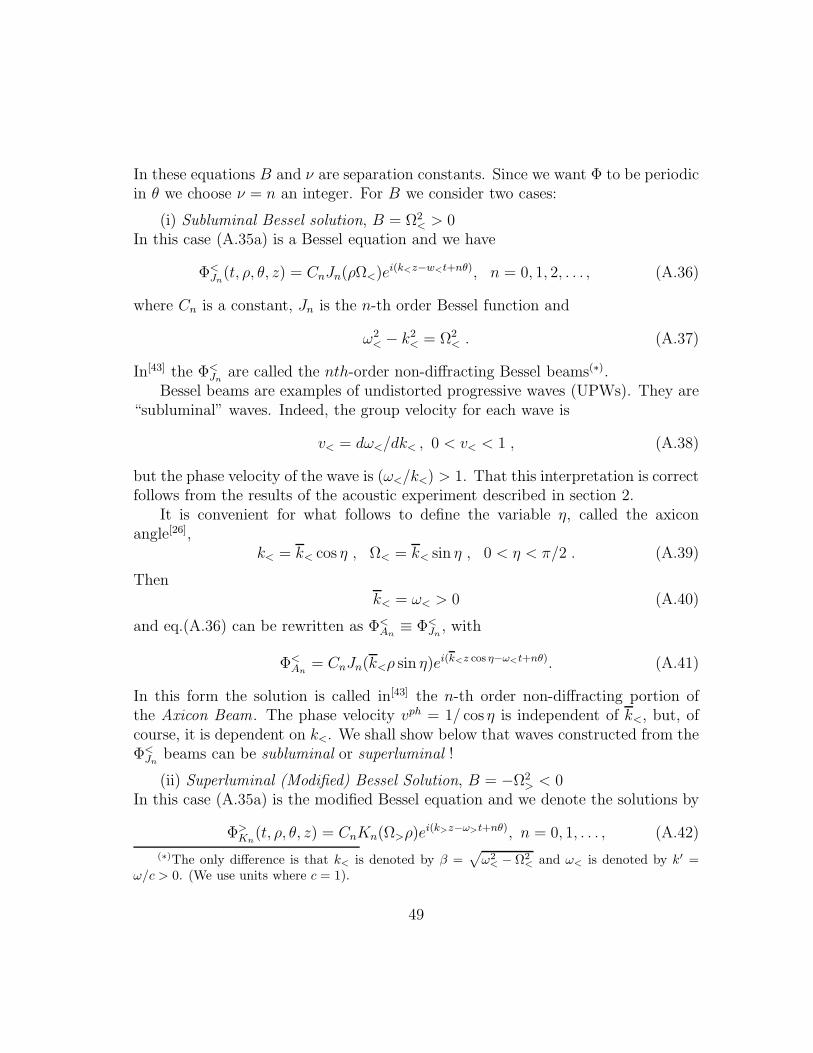
In these equations B and ν are separation constants. Since we want Φ to be periodicin θ we choose ν = n an integer. For B we consider two cases:

(i) Subluminal Bessel solution, B = Ω2< > 0

In this case (A.35a) is a Bessel equation and we have

Φ<Jn

(t, ρ, θ, z) = CnJn(ρΩ<)ei(k<z−w<t+nθ), n = 0, 1, 2, . . . , (A.36)

where Cn is a constant, Jn is the n-th order Bessel function and

ω2< − k2

< = Ω2< . (A.37)

In[43] the Φ<Jn

are called the nth-order non-diffracting Bessel beams(∗).Bessel beams are examples of undistorted progressive waves (UPWs). They are

“subluminal” waves. Indeed, the group velocity for each wave is

v< = dω</dk< , 0 < v< < 1 , (A.38)

but the phase velocity of the wave is (ω</k<) > 1. That this interpretation is correctfollows from the results of the acoustic experiment described in section 2.

It is convenient for what follows to define the variable η, called the axiconangle[26],

k< = k< cos η , Ω< = k< sin η , 0 < η < π/2 . (A.39)

Thenk< = ω< > 0 (A.40)

and eq.(A.36) can be rewritten as Φ<An

≡ Φ<Jn

, with

Φ<An

= CnJn(k<ρ sin η)ei(k<z cos η−ω<t+nθ). (A.41)

In this form the solution is called in[43] the n-th order non-diffracting portion ofthe Axicon Beam. The phase velocity vph = 1/ cos η is independent of k<, but, ofcourse, it is dependent on k<. We shall show below that waves constructed from theΦ<

Jnbeams can be subluminal or superluminal !

(ii) Superluminal (Modified) Bessel Solution, B = −Ω2> < 0

In this case (A.35a) is the modified Bessel equation and we denote the solutions by

Φ>Kn

(t, ρ, θ, z) = CnKn(Ω>ρ)ei(k>z−ω>t+nθ), n = 0, 1, . . . , (A.42)

(∗)The only difference is that k< is denoted by β =√

ω2< − Ω2

< and ω< is denoted by k′ =ω/c > 0. (We use units where c = 1).

49

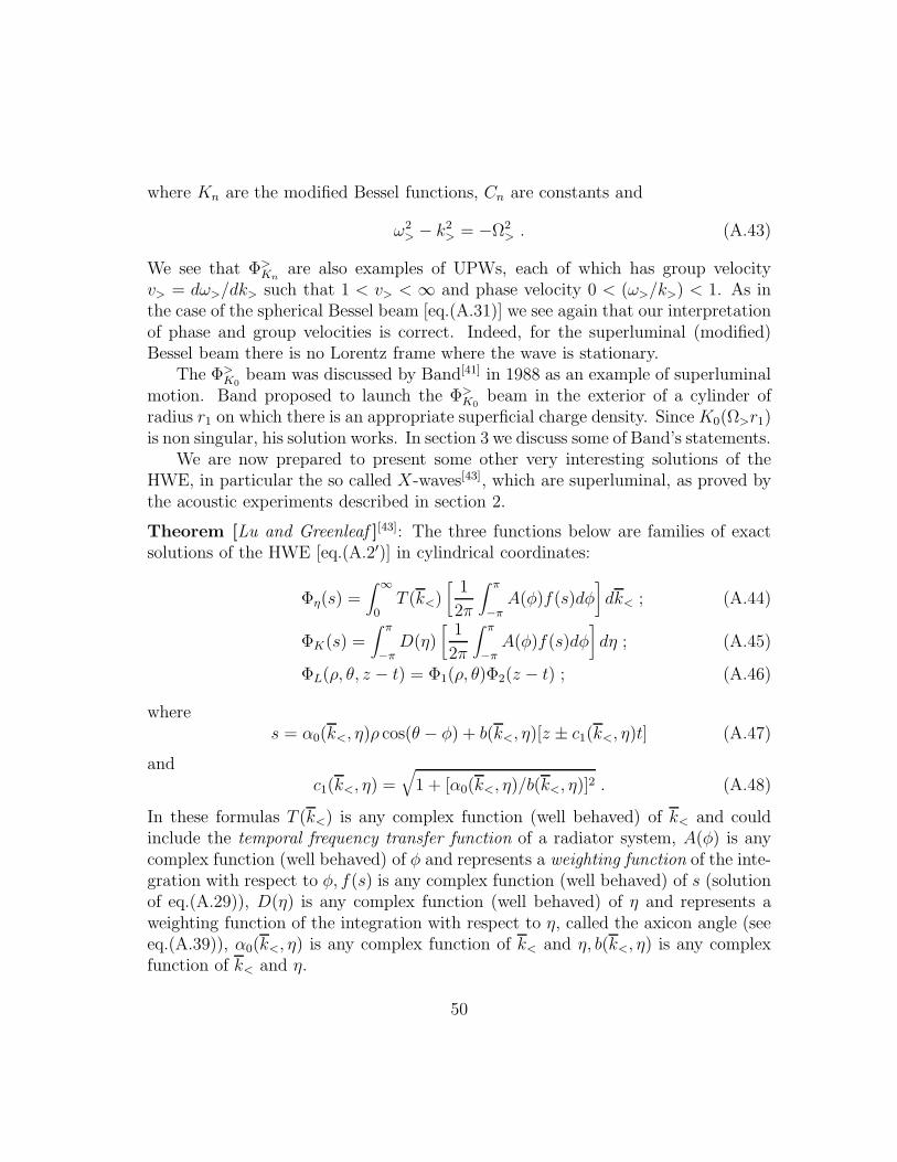
where Kn are the modified Bessel functions, Cn are constants and

ω2> − k2

> = −Ω2> . (A.43)

We see that Φ>Kn

are also examples of UPWs, each of which has group velocityv> = dω>/dk> such that 1 < v> < ∞ and phase velocity 0 < (ω>/k>) < 1. As inthe case of the spherical Bessel beam [eq.(A.31)] we see again that our interpretationof phase and group velocities is correct. Indeed, for the superluminal (modified)Bessel beam there is no Lorentz frame where the wave is stationary.

The Φ>K0

beam was discussed by Band[41] in 1988 as an example of superluminalmotion. Band proposed to launch the Φ>

K0beam in the exterior of a cylinder of

radius r1 on which there is an appropriate superficial charge density. Since K0(Ω>r1)is non singular, his solution works. In section 3 we discuss some of Band’s statements.

We are now prepared to present some other very interesting solutions of theHWE, in particular the so called X-waves[43], which are superluminal, as proved bythe acoustic experiments described in section 2.

Theorem [Lu and Greenleaf ][43]: The three functions below are families of exactsolutions of the HWE [eq.(A.2′)] in cylindrical coordinates:

Φη(s) =∫ ∞

0T (k<)

[1

2π

∫ π

−πA(φ)f(s)dφ

]dk< ; (A.44)

ΦK(s) =∫ π

−πD(η)

[1

2π

∫ π

−πA(φ)f(s)dφ

]dη ; (A.45)

ΦL(ρ, θ, z − t) = Φ1(ρ, θ)Φ2(z − t) ; (A.46)

wheres = α0(k<, η)ρ cos(θ − φ) + b(k<, η)[z ± c1(k<, η)t] (A.47)

andc1(k<, η) =

√1 + [α0(k<, η)/b(k<, η)]2 . (A.48)

In these formulas T (k<) is any complex function (well behaved) of k< and couldinclude the temporal frequency transfer function of a radiator system, A(φ) is anycomplex function (well behaved) of φ and represents a weighting function of the inte-gration with respect to φ, f(s) is any complex function (well behaved) of s (solutionof eq.(A.29)), D(η) is any complex function (well behaved) of η and represents aweighting function of the integration with respect to η, called the axicon angle (seeeq.(A.39)), α0(k<, η) is any complex function of k< and η, b(k<, η) is any complexfunction of k< and η.

50

As in the previous solutions, we take c = 1. Note that k<, η and the wave vectork< of the f(s) solution of eq.(A.29) are related by eq.(A.39). Also Φ2(z − t) is anycomplex function of (z − t) and Φ1(ρ, θ) is any solution of the transverse Laplaceequation, i.e., [

1

ρ

∂

∂ρ

(ρ∂

∂ρ

)+

1

ρ2

∂2

∂θ2

]Φ1(ρ, θ) = 0. (A.49)

The proof is obtained by direct substitution of Φη, ΦK and ΦL in the HWE. Ob-viously, the exact solution ΦL is an example of a luminal UPW, because if one“travels” with the speed c = 1, i.e., with z − t = const., both the lateral and axialcomponents Φ1(ρ, θ) and Φ2(z − t) will be the same for all time t and distance z.When c1(k, η) in eq.(A.47) is real, (±) represent respectively backward and forwardpropagating waves.

We recall that Φη(s) and ΦK(s) represent families of UPWs if c1(k<, η) is inde-pendent of k< and η respectively. These waves travel to infinity at speed c1. Φη(s)is a generalized function that contains some of the UPWs solutions of the HWEderived previously. In particular, if T (k<) = δ(k< − k

′

<), k′

< = ω > 0 is a constantand if f(s) = es, α0(k<, η) = −iΩ<, b(k<, η) = iβ = iω/c1, one obtains Durnin’sUPW beam[16]

ΦDurnin(s) =[

1

2π

∫ π

−πA(φ)e−iΩ<ρ cos(θ−φ)dφ

]ei(βz−ωt). (A.50)

If A(φ) = ineinφ we obtain the n-th order UPW Bessel beam Φ<Jn

given by eq.(A.36).Φ<

An(s) is obtained in the same way with the transformation k< = k< cos η; Ω< =

k< sin η.

The X-waves. We now present a superluminal UPW wave which, as discussedin section 2, is physically realizable in an approximate way (FAA) in the acousticcase and can be used to generate Hertz potentials for the electromagnetic field (seesection 3). We take in eq.(A.44):

T (k<) = B(k<)e−a0k<; A(φ) = ineinφ; α0(k<, η) = −ik< sin η;

b(k<, η) = ik cos η; f(s) = es. (A.51)

We then get

Φ>Xn

= einθ∫ ∞

0B(k<)Jn(k<ρ sin η)e−k<[a0−i(z cos η−t)]dk< . (A.52)

51

In eq.(A.52) B(k<) is any well behaved complex function of k< and represents atransfer function of practical radiator, k< = ω and a0 is a constant, and η is againcalled the axicon angle[26]. Eq.(A.52) shows that Φ>

Xnis represented by a Laplace

transform of the function B(k<)Jn(k<ρ sin η) and an azimuthal phase term einθ.The name X-waves for the Φ>

Xncomes from the fact that these waves have an X-

like shape in a plane containing the axis of symmetry of the waves (the z-axis, seeFig.4(1) in section 3).

The Φ>XBBn

waves. This wave is obtained from eq.(A.44) putting B(k<) = a0. Itis called the X-wave produced by an infinite aperture and broad bandwidth. We usein this case the notation Φ>

XBBn. Under these conditions we get

Φ>XBBn

=a0(ρ sin η)neinθ

√M(τ +

√M)n

, (n = 0, 1, 2, . . .) (A.53)

where the subscript denotes “broadband”. Also

M = (ρ sin η)2 + τ 2 ; (A.54)

τ = [a0 − i(z cos η − t)] (A.55)

For n = 0 we get Φ>XBB0

:

Φ>XBB0

=a0√

(ρ sin η)2 + [a0 − i(z cos η − t)]2. (A.56)

It is clear that all Φ>XBBn

are UPWs which propagate with speed c1 = 1/ cos η > 1in the z-direction. Our statement is justified for as can be easily seen (as in themodified superluminal Bessel beam) there is no Lorentz frame where Φ>

XBBnis at

rest. Observe that this is the real speed of the wave; phase and group velocityconcepts are not applicable here. Eq(A.56) does not give any dispersion relation.

The Φ>XBBn

waves cannot be produced in practice as they have infinite energy(see section A7), but as we shall show a good approximation for them can be realizedwith finite aperture radiators.

A5. Construction of Φ<Jn

and X-Waves with Finite Aperture Radiators

In section A3 we study the condition under which the Rayleigh-Sommerfeldsolution to HWE [eq.(A.24)] can be derived. The condition is just that the wave Φ

52

must be written as Φ(t, ~x) = F (~x)e−iωt; which is true for the Bessel beams Φ<Jn

. Insection 2 we show that a finite aperture approximation (FAA) to a broad band Besselbeam or Bessel pulse denoted FAAΦBBJn

or ΦFAJn[see eq.(2.3)] can be physically

realized and moves as predicted by the theory.At first sight it is not obvious that for the ΦXn

waves we can use eq.(A.26), butactually we can. This happens because we can write,

Φ>Xn

(t, ~x) =1

2π

∫ +∞

−∞

˜Φ

>

Xn(ω, ~x)e−iωtdω (A.57)

˜Φ

>

Xn(ω, ~x) = 2πeinθB(ω)Jn(ωρ sin η)H(ω)e−ω(a0−iz cos η), n = 0, 1, 2, . . .(A.58)

where H(ω) is the step function and each˜ΦXn

(ω, ~x) is a solution of the transverseHelmholtz equation. Then the Rayleigh-Sommerfeld approximation can be writtenand the FAA can be used. Denoting the FAA to Φ>

Xnby Φ>

FAXnand using eq.(A.28)

we get

Φ>FAXn

(k<, ~x) =1

iλ

∫ 2π

0dθ′

∫ D/2

0ρ′dρ′

˜ΦXn

(k<, ρ′, φ′)

eik<R

R2z

+1

2π

∫ 2π

0dθ′

∫ D/2

0ρ′dρ′

˜ΦXn

(k<, ρ′, θ′)

eik<R

R3z ; (A.59)

Φ>FAXn

(t, ~x) = F−1[Φ>FAXn

(ω, ~x)], n = 0, 1, 2, . . . , (A.60)

where λ is the wave length and R = |~x − ~x′|. F−1 represents the inverse Fouriertransform. The first and second terms in eq.(A.59) represent respectively the con-tributions from high and low frequency components. We attached the symbol > toΦ>

FAXnmeaning as before that the wave is superluminal. This is justified from the

results of the experiment described in section 2.

A6. The Donnelly-Ziolkowski Method (DZM) for Designing Subluminal,Luminal and Superluminal UPWs Solutions of the HWE and the Klein-Gordon Equation (KGE)

Consider first the HWE for Φ [eq.(A.2′)] in a homogeneous medium. Let Φ(ω,~k)be the Fourier transform of Φ(t, ~x), i.e.,

Φ(ω,~k) =∫

R3

d3x∫ +∞

−∞dtΦ(t, ~x)e−i(~k~x−ωt) , (A.61a)

53

Φ(t, ~x) =1

(2π)4

∫

R3

d3~k∫ +∞

−∞dω Φ(ω,~k)ei(~k~x−ωt). (A.61b)

Inserting (A.61a) in the HWE we get

(ω2 − ~k2)Φ(ω,~k) = 0 (A.62)

and we are going to look for solutions of the HWE and eq.(A.62) in the sense ofdistributions. We rewrite eq.(A.62) as

(ω2 − k2z − Ω2)Φ(ω,~k) = 0. (A.63)

It is then obvious that any Φ(ω,~k) of the form

Φ(ω,~k) = Ξ(Ω, β) δ[ω − (β + Ω2/4β)] δ[kz − (β − Ω2/4β)] , (A.64)

where Ξ(Ω, β) is an arbitrary weighting function, is a solution of eq.(A.63) since theδ-functions imply that

ω2 − k2z = Ω2 . (A.65)

In 1985[30] Ziolkowski found a luminal solution of the HWE called the FocusWave Mode. To obtain this solution we choose, e.g.,

ΞFWM(Ω, β) =π2

iβexp(−Ω2z0/4β), (A.66)

whence we get, assuming β > 0 and z0 > 0,

ΦFWM(t, ~x) = eiβ(z+t) exp−ρ2β/[z0 + i(z − t)]4πi[z0 + i(z − t)]

. (A.67)

Despite the velocities v1 = +1 and v2 = −1 appearing in the phase, the modulationfunction of ΦFWM has very interesting properties, as discussed in details in [46]. Itremains to observe that eq.(A.67) is a special case of Brittingham’s formula.[26]

Returning to eq.(A.64) we see that the δ-functions make any function of theFourier transform variables ω, kz and Ω to lie in a line on the surface ω2−k2

z −Ω2 = 0[eq.(A.63)]. Then, the support of the δ-functions is the line

ω = β + Ω2/4β; kz = β − Ω2/4β . (A.68)

The projection of this line in the (ω, kz) plane is a straight line of slope −1 endingat the point (β, β). When β = 0 we must have Ω = 0, and in this case the line

54

is ω = kz and Φ(t, ~x) is simply a superposition of plane waves, each one havingfrequency ω and traveling with speed c = 1 in the positive z direction.

Luminal UPWs solutions can be easily constructed by the ZM[46], but will notbe discussed here. Instead, we now show how to use ZM to construct subluminaland superluminal solutions of the HWE.

First Example: Reconstruction of the subluminal Bessel Beams Φ<J0

and the su-perluminal Φ>

XBB0(X-wave)

Starting from the “dispersion relation” ω2 − k2z − Ω2 = 0, we define

Φ(ω, k) = Ξ(k, η)δ(kz − k cos η)δ(ω − k). (A.69)

This implies that

kz = k cos η; cos η = kz/ω, ω > 0, −1 < cos η < 1 . (A.70)

We take moreoverΩ = k sin η; k > 0 . (A.71)

We recall that ~Ω = (kx, ky), ~ρ = (x, y) and we choose ~Ω.~ρ = Ωρ cos θ. Now,putting eq.(A.69) in eq.(A.61b) we get

Φ(t, ~x) =1

(2π)4

∫ ∞

0dk k sin2 η

[∫ 2π

0dθ Ξ(k, η) eikρ sin η cos θ

]ei(k cos ηz−kt). (A.72)

Choosing

Ξ(k, η) = (2π)3 z0e−kz0 sin η

k sin η, (A.73)

where z0 > 0 is a constant, we obtain

Φ(t, ~x) = z0 sin η∫ ∞

0dk e−kz0 sin η

[1

2π

∫ 2π

0dθ eikρ sin η cos θ

]eik(cos η z−t) .

Calling z0 sin η = a0 > 0, the last equation becomes

Φ>X0

(t, ~x) = a0

∫ ∞

0dk e−ka0J0(kρ sin η)eik(cos η z−t). (A.74)

Writing k = k< and taking into account eq.(A.41) we see that

J0(k<ρ sin η)eik<(z cos η−t) (A.75)

55

is a subluminal Bessel beam, a solution of the HWE moving in the positive z di-rection. Moreover, a comparison of eq.(A.74) with eq.(A.52) shows that (A.74) is

a particular superluminal X-wave, with B(k<) = e−a0k<. In fact it is the Φ>XBB0

UPW given by eq.(A.56).

Second Example: Choosing in (A.72)

Ξ(k, η) = (2π)3e−z0| cos η|k cot η (A.76)

gives

Φ>(t, ~x) = cos2 η∫ ∞

0dk ke−z0| cos η|kJ0(kρ sin η)e−ik(cos ηz−t) (A.77a)

=[z0 − isgn(cos η)(z − t/ cos η)]

[ρ2 tan2 η + [z0 + isgn(cos η)(z − t/ cos η)]2]3/2. (A.77b)

Comparing eq.(A.77a) with eq.(A.52) we discover that the ZM produced in this

example a more general Φ>X0

wave where B(k<) = e−z0| cos η|k< . Obviously Φ>(t, ~x)given by eq.(A.77b) moves with superluminal speed (1/cos η) in the positive ornegative z-direction depending on the sign of cos η, denoted sgn(cos η).

In both examples studied above we see that the projection of the supportingline of eq.(A.69) in the (ω, kz) plane is the straight line kz/ω = cos η, and cos η isits reciprocal slope. This line is inside the “light cone” in the (ω, kz) plane.

Third Example: Consider two arbitrary lines with the same reciprocal slope thatwe denote by v > 1, both running between the lines ω = ±kz in the upper half planeω > 0 and each one cutting the ω-axis at different values β1 and β2 (Fig.(12)). Thetwo lines are projections of members of a family of HWE solution lines and each onecan be represented as a portion of the straight lines (between the lines ω = ±kz)

kz = v(ω − β1), kz = v(ω − β2). (A.78)

It is clear that on the solution line of the HWE, Ω takes values from zero up to amaximum value that depends on v and β and then back to zero.

We see also that the maximum value of Ω, given by βv/√v2 − 1, on any HWE

solution line occurs for those values of ω and kz where the corresponding projectionlines cut the line ω = vkz. It is clear that there are two points on any HWE solutionline with the same value of Ω in the interval

0 < Ω < vβ/√v2 − 1 = Ω0. (A.79)

56

It follows that in this case the HWE solution line breaks into two segments, as is thecase of the projection lines. We can then associate two different weighting functions,one for each segment. We write

Φ(Ω, ω, kz) = Ξ1(Ω, v, β) δ

kz −

v[β +√β2v2 − Ω2(v2 − 1)]

(v2 − 1)

×

×δω −

[βv2 +√v2β2 − Ω2(v2 − 1)]

(v2 − 1)

+

+ Ξ2(Ω, v, β) δ

kz −

v[β −√β2v2 − Ω2(v2 − 1)]

(v2 − 1)

×

× δ

ω −[βv2 −

√v2β2 − Ω2(v2 − 1)]

(v2 − 1)

. (A.80)

Now, choosing

Ξ1(Ω, v, β) = Ξ2(Ω, v, β) = (2π)3/2√

Ω20 − Ω2

we get

Φv,β(t, ρ, z) = Ω0 exp

(iβv(z − vt)√

v2 − 1

) ∫ ∞

0dχ χJ0(Ω0ρχ) cos

Ω0v√v2 − 1

(z − t/v)√1 − χ2

.

Then

Φv,β(t, ρ, z) = exp

[iβv(z − vt)√v2 − 1

]sin

Ω0

√v2

(v2−1)(z − t/v)2 + ρ2

Ω0

√v2

(v2−1)(z − t/v)2 + ρ2

. (A.81)

If we call v< =1

v< 1 and taking into account the value of Ω0 given by eq.(A.79),

we can write eq.(A.81) as

Φv<(t, ρ, z) =

sin(Ω0ξ<)

ξ<eiΩ0(z−vt) ;

ξ< =

[x2 + y2 +

1

1 − v2<

(z − v<t)2

]1/2

; (A.82)

which we recognize as the subluminal spherical Bessel beam of section A4 [eq.(A.31)].

57

Figure 12: Projection of the support lines of the transforms of two members of afamily of subluminal solutions of the HWE.

Klein-Gordon Equation (KGE): We show here the existence of subluminal, lu-minal and superluminal UPW solutions of the KGE. We want to solve

(∂2

∂t2−∇2 +m2

)ΦKG(t, ~x) = 0, m > 0, (A.83)

with the Fourier transform method. We obtain for ΦKG(ω,~k) (a generalized func-tion) the equation

ω2 − k2z − (Ω2 +m2)ΦKG(ω,~k) = 0. (A.84)

As in the case of the HWE, any solution of the KGE will have a transformΦ(ω,~k) such that its support line lies on the surface

ω2 − k2z − (Ω2 +m2) = 0 . (A.85)

From eq.(A.85), calling Ω2 + m2 = K2, we see that we are in a situation identicalto the HWE for which we showed the existence of subluminal, superluminal andluminal solutions. We write down as examples one solution of each kind.

58

Subluminal UPW solution of the KGE. To obtain this solution it is enough to

change in eq.(A.81) Ω0 = vβ/√v2 − 1 → ΩKG

0 =

(

vβ√v2 − 1

)2

−m2

1/2

. We have

ΦKG< (t, ρ, z) = exp

iβv(z − vt)√

v2 − 1

sin(ΩKG

0 ξ<)

ξ<;

ξ< =

[x2 + y2 +

1

1 − v2<

(z − v<t)2

]1/2

, v< = 1/v. (A.86)

Luminal UPW solution of the KGE. To obtain a solution of this type it is enough,as in eq.(A.64), to write

ΦKG = Ξ(Ω, β)δ[kz − (Ω2 + (m2 − β2)/2β)]δ[ω − (Ω2 + (m2 + β2)/2β)] . (A.87)

Choosing

Ξ(Ω, β) =(2π)2

βexp(−z0Ω2/2β), z0 > 0, (A.88)

gives

ΦKGβ (t, ~x) =

= exp(iz(m2 − β2)/2β) exp(−it(m2 + β)/2β)exp−ρ2β/2[z0 − i(z − t)]

[z0 − i(z − t)]. (A.89)

Superluminal UPW solution of the KGE. To obtain a solution of this kind weintroduce a parameter v such that 0 < v < 1 and write for ΦKG in (A.84)

ΦKGv,β (ω,Ω, kz) = Ξ(Ω, v, β) δ

ω −

(−βv2 +

√(Ω2 +m2)(1 − v2) + v2β2

)

1 − v2

×

×δ

kz −

v(−β +

√(Ω2 +m2)(1 − v2) + v2β2

)

1 − v2

. (A.90)

Next we choose

Ξ(Ω, v, β) =(2π)3 exp(−z0

√Ω2

0 + Ω2)√

Ω20 + Ω2

, (A.91)

59

where z0 > 0 is an arbitrary parameter, and where

Ω20 =

β2v2

1 − v2+m2 . (A.92)

Then introducing v> = 1/v > 1 and γ> =1

√v2

> − 1, we get

ΦKG>

v,β (t, ~x) = exp

i(Ω2

0 −m2)(z − vt)

βv

exp−Ω0

√[z0 − iγ>(z − v>t)]2 + x2 + y2

√[z0 − iγ>(z − v>t)]2 + x2 + y2

,

(A.93)which is a superluminal UPW solution of the KGE moving with speed v> in the zdirection. From eq.(A.93) it is an easy task to reproduce the superluminal sphericalBessel beam which is solution of the HWE [eq.(A.30)].

A7. On the Energy of the UPWs Solutions of the HWE

Let Φr(t, ~x) be a real solution of the HWE. Then, as it is well known, the energyof the solution is given by

ε =∫ ∫ ∫

IR3

dv

(∂Φr

∂t

)2

− Φr∇2Φr

+ lim

R→∞

∫ ∫

S(R)dS Φr ~n.∇Φr , (A.94)

where S(R) is the 2-sphere of radius R .We can easily verify that the real or imaginary parts of all UPWs solutions of the

HWE presented above have infinite energy. The question arises of how to projectsuperluminal waves, solutions of the HWE, with finite energy. This can be done ifwe recall that all UPWs discussed above can be indexed by at least one parameterthat here we call α. Then, calling Φα(t, ~x) the real or imaginary parts of a givenUPW solution we may form “packets” of these solutions as

Φ(t, ~x) =∫dαF (α)Φα(t, ~x) (A.95)

We now may test for a given solution Φα and for a weighting function F (α) ifthe integral in eq.(A.94) is convergent. We can explicitly show for some (but notall) of the solutions showed above (subluminal, luminal and superluminal) that forweighting functions satisfying certain integrability conditions the energy ε results

60

finite. It is particularly important in this context to quote that the finite apertureapproximations for all UPWs have, of course, finite energy. For the case in which Φgiven by eq.(A.95) is used to generate solutions for, e.g., Maxwell or Dirac fields (seeAppendix B), the conditions for the energy of these fields to be finite will in generalbe different from the condition that gives for Φ a finite energy. This problem willbe discussed with more details in another paper.

Appendix B. A Unified Theory for Construction of UPWsSolutions of Maxwell, Dirac and Weyl Equations

In this appendix we briefly recall the main results concerning the theory of Clif-ford algebras (and bundles) and their relationship with the Grassmann algebras(and bundles). Also the concept of Dirac-Hestenes spinors and their relationshipwith the usual Dirac spinors used by physicists is clarified. We introduce moreoverthe concepts of the Clifford and Spin-Clifford bundles of spacetime and the Cliffordcalculus. As we shall see, this formalism provides a unified theory for the construc-tion of UPWs subluminal, luminal and superluminal solutions of Maxwell, Dirac andWeyl equations. More details on the topics of this appendix can be found in[6−9]

and[81].

B1. Mathematical PreliminariesLet M = (M, g,D) be Minkowski spacetime. (M, g) is a four-dimensional

time oriented and space oriented Lorentzian manifold, with M ≃ IR4 and g ∈

sec(T ∗M × T ∗M) being a Lorentzian metric of signature (1,3). T ∗M [TM ] isthe cotangent [tangent] bundle. T ∗M = ∪x∈MT

∗xM and TM = ∪x∈MTxM , and

TxM ≃ T ∗xM ≃ IR1,3, where IR

1,3 is the Minkowski vector space[60,61,62]. D is theLevi-Civita connection of g, i.e., Dg = 0, T (D) = 0. Also R(D) = 0, T and Rbeing respectively the torsion and curvature tensors. Now, the Clifford bundle ofdifferential forms Cℓ(M) is the bundle of algebras Cℓ(M) = ∪x∈MCℓ(T ∗xM), where∀x ∈M, Cℓ(T ∗xM) = Cℓ1,3, the so called spacetime algebra[9,81−85]. Locally as a linearspace over the real field IR, Cℓ(T ∗x (M)) is isomorphic to the Cartan algebra

∧(T ∗xM)

of the cotangent space and∧

(T ∗xM) =∑4

k=0

∧ k(T ∗xM), where∧k(T ∗xM) is the

(4k

)-

dimensional space of k-forms. The Cartan bundle∧

(M) = ∪x∈M∧

(T ∗xM) can thenbe thought as “embedded” in Cℓ(M). In this way sections of Cℓ(M) can be repre-sented as a sum of inhomogeneous differential forms. Let eµ = ∂

∂xµ ∈ sec TM ,(µ = 0, 1, 2, 3) be an orthonormal basis g(eµ, eν) = ηµν = diag(1,−1,−1,−1) and

61

let γν = dxν ∈ sec∧1(M) ⊂ sec Cℓ(M) be the dual basis. Then, the fundamental

Clifford product (denoted in what follows by juxtaposition of symbols) is generatedby γµγν + γνγµ = 2ηµν and if C ∈ secCℓ(M) we have

C = s+ vµγµ +

1

2!bµνγ

µγν +1

3!aµνργ

µγνγρ + pγ5 , (B.1)

where γ5 = γ0γ1γ2γ3 = dx0dx1dx2dx3 is the volume element and s, vµ, bµν , aµνρ,p ∈ sec

∧0(M) ⊂ sec Cℓ(M). For Ar ∈ sec∧r(M) ⊂ sec Cℓ(M), Bs ∈ sec

∧s(M)we define[9,82] Ar · Bs = 〈ArBs〉|r−s| and Ar ∧ Bs = 〈ArBs〉r+s, where 〈 〉k is thecomponent in

∧k(M) of the Clifford field.Besides the vector bundle Cℓ(M) we also need to introduce another vector bundle

CℓSpin+(1,3)(M) [Spin+(1, 3) ≃ SL(2, IC)] called the Spin-Clifford bundle[8,81,84]. Wecan show that CℓSpin+(1,3)(M) ≃ Cℓ(M)/R, i.e. it is a quotient bundle. This meansthat sections of CℓSpin+(1,3)(M) are equivalence classes of sections of the Cliffordbundle, i.e., they are equivalence sections of non-homogeneous differential forms(see eqs.(B.2,B.3) below).

Now, as is well known, an electromagnetic field is represented by F ∈ sec∧2(M) ⊂

sec Cℓ(M). How to represent the Dirac spinor fields in this formalism ? We can showthat the even sections of CℓSpin+(1,3)(M), called Dirac-Hestenes spinor fields, do the

job. If we fix two orthonormal basis Σ = γµ as before, and Σ = γµ = RγµR =Λµ

νγν with Λµ

ν ∈ SO+(1, 3) and R(x) ∈ Spin+(1, 3) ∀x ∈ M , RR = RR = 1, andwhere ˜ is the reversion operator in Cℓ1,3, then[8,81] the representatives of an evensection ψ ∈ sec CℓSpin+(1,3)(M) are the sections ψΣ and ψΣ of Cℓ(M) related by

ψΣ = ψΣR (B.2)

and

ψΣ = s+1

2!bµνγ

µγν + pγ5. (B.3)

Note that ψΣ has the correct number of degrees of freedom in order to represent aDirac spinor field, which is not the case with the so called Dirac-Kahler spinor field(see[8,81]).

Let ⋆ be the Hodge star operator ⋆ :∧k(M) → ∧4−k(M). We can show that

if Ap ∈ sec∧p(M) ⊂ sec Cℓ(M) we have ⋆A = Aγ5. Let d and δ be respectively

the differential and Hodge codifferential operators acting on sections of∧

(M). Ifωp ∈ sec

∧p(M) ⊂ sec Cℓ(M), then δωp = (−1)p ⋆−1 d ⋆ ωp, with ⋆−1⋆ = identity.The Dirac operator acting on sections of Cℓ(M) is the invariant first order dif-

ferential operator∂ = γµDeµ

, (B.4)

62

and we can show the very important result (see e.g.[6]):

∂ = ∂ ∧ +∂· = d− δ. (B.5)

With these preliminaries we can write Maxwell and Dirac equations as follows[82,85]:

∂F = 0, (B.6)

∂ψΣγ1γ2 +mψΣγ

0 = 0. (B.7)

We discuss more this last equation (Dirac-Hestenes equation) in section B.4. Ifm = 0 we have the massless Dirac equation

∂ψΣ = 0, (B.8)

which is Weyl’s equation when ψΣ is reduced to a Weyl spinor field (see eq.(B.12 be-low). Note that in this formalism Maxwell equations condensed in a single equation!Also, the specification of ψΣ depends on the frame Σ. When no confusion arises werepresent ψΣ simply by ψ.

When ψΣψΣ 6= 0, where ∼ is the reversion operator, we can show that ψΣ hasthe following canonical decomposition:

ψΣ =√ρ eβγ5/2R , (B.9)

where ρ, β ∈ sec∧0(M) ⊂ sec Cℓ(M) and R ∈ Spin+(1, 3) ⊂ Cℓ+1,3, ∀x ∈ M . β is

called the Takabayasi angle[8].If we want to work in terms of the usual spinor field formalism, we can translate

our results by choosing, for example, the standard matrix representation of γµ, andfor ψΣ given by eq.(B.3) we have the following (standard) matrix representation[8,49]:

Ψ =

(φ1 −φ∗2φ2 φ∗1

), (B.10)

where

φ1 =

(s− ib12 b13 − ib23

−b13 − ib23 s+ ib12

), φ2 =

(−b03 + ip −b01 + ib02−b01 − ib02 b03 + ip

), (B.11)

with s, b12, . . . real functions; ∗ denotes the complex conjugation. Right multiplica-tion by

1000

63

gives the usual Dirac spinor field.We need also the concept of Weyl spinors. By definition, ψ ∈ sec Cℓ+(M) is a

Weyl spinor if[83]

γ5ψ = ±ψγ21 . (B.12)

The positive [negative] “eigenstate” of γ5 will be denoted ψ+ [ψ−]. For a generalψ ∈ sec Cℓ+(M) we can verify that

ψ± =1

2[ψ ∓ γ5ψγ21] (B.13)

are Weyl spinors with eigenvalues ±1 of eq.(B.12).We recall that the even subbundle Cℓ+(M) of Cℓ(M) is such that its typical fiber

is the Pauli algebra Cℓ3,0 ≡ Cℓ+1,3 (which is isomorphic to IC(2), the algebra of 2 × 2complex matrices). The isomorphism Cℓ3,0 ≡ Cℓ+1,3 is exhibited by putting σi = γiγ0,

whence σiσj + σjσi = 2δij. We recall also[8,81] that the Dirac algebra is Cℓ4,1 ≡ IC(4)(see section B4) and Cℓ4,1 ≡ IC ⊗ Cℓ1,3

[86].

B2. Inertial Reference Frames (I), Observers and Naturally AdaptedCoordinate Systems

Let M = (M, g,D) be Minkowski spacetime. An inertial reference frame (irf)I is a timelike vector field I ∈ secTM pointing into the future such that g(I, I) = 1and DI = 0. Each integral line of I is called an inertial observer. The coordinatefunctions 〈xµ〉, µ = 0, 1, 2, 3 of the maximal atlas of M are said to be a naturallyadapted coordinate system to I (nacs/I) if I = ∂/∂x0 [61,62]. Putting I = e0 we canfind ei = ∂/∂xi, i = 1, 2, 3 such that g(eµ, eν) = ηµν and the coordinate functionsxµ are the usual Einstein-Lorentz ones and have a precise operational meaning:x0 = ct(∗), where t is measured by “ideal clocks” at rest on I and synchronized “a laEinstein”, xi, i = 1, 2, 3 are determined with ideal rules[61,62]. (We use units wherec = 1.)

B3. Maxwell Theory in Cℓ(M) and the Hertz Potential

Let eµ ∈ sec TM be an orthonormal basis, g(eµ, eν) = ηµν and eµ = ∂/∂xµ

(µ, ν = 0, 1, 2, 3), such that e0 determines an IRF. Let γµ ∈ sec∧2(M) ⊂ sec Cℓ(M)

(∗)c is the constant called velocity of light in vacuum. In view of the superluminal and sub-luminal solutions of Maxwell equations found in this paper we don’t think the terminology to bestill satisfactory.

64

be the dual basis and let γµ = ηµνγν be the reciprocal basis to γµ, i.e., γµ.γν = δµ

ν .We have γµ = dxµ.

As is well known the electromagnetic field is represented by a two-form F ∈sec

∧2(M) ⊂ sec Cℓ(M). We have

F =1

2F µνγµγν , F

µν =

0 −E1 −E2 −E3

E1 0 −B3 B2

E2 B3 0 −B1

E3 −B2 B1 0

, (B.14)

where (E1, E2, E3) and (B1, B2, B3) are respectively the Cartesian components ofthe electric and magnetic fields. Let J ∈ sec

∧1(M) ⊂ sec Cℓ(M) be such that

J = Jµγµ = ργ0 + J1γ1 + J2γ2 + J3γ3, (B.15)

where ρ and (J1, J2, J3) are respectively the Cartesian components of the chargeand of the three-dimensional current densities.

We now write Maxwell equation given by B.6 in Cℓ+(M), the even sub-algebraof Cℓ(M). The typical fiber of Cℓ+(M), which is a vector bundle, is isomorphic tothe Pauli algebra (see section B1). We put

~σi = γiγ0, i = ~σ1~σ2~σ3 = γ0γ1γ2γ3 = γ5. (B.16)

Recall that i commutes with bivectors and since i2 = −1 it acts like the imagi-nary unit i =

√−1 in Cℓ+(M). From eq.(B.14), we get

F = ~E + i ~B (B.17)

with ~E = Ei~σi, ~B = Bj~σj , i, j = 1, 2, 3. Now, since ∂ = γµ∂µ we get ∂γ0 =

∂/∂x0 + ~σi∂i = ∂/∂x0 −∇. Multiplying eq.(B.6) on the right by γ0 we have

∂γ0γ0Fγ0 = Jγ0,

(∂/∂x0 −∇)(−~E + i ~B) = ρ+ ~J, (B.18)

where we used γ0Fγ0 = −~E + i ~B and ~J = J i~σi. From eq.(B.18) we have

−∂0~E + i∂0

~B + ∇ ~E − i∇ ~B = ρ+ ~J (B.19)

−∂0~E + i∂0

~B + ∇. ~E + ∇∧ ~E − i∇. ~B − i∇ ∧ ~B = ρ+ ~J (B.20)

65

We have also− i∇ ∧ ~A ≡ ∇× ~A (B.21)

since the usual vector product between two vectors ~a = ai~σi, ~b = bi~σi can beidentified with the dual of the bivector ~a ∧~b through the formula ~a ×~b = −i(~a ∧~b). Observe that in this formalism ~a ×~b is a true vector and not the meaninglesspseudovector of the Gibbs vector calculus. Using eq.(B.21) and equating the termswith the same grade we obtain

∇. ~E = ρ ; ∇× ~B − ∂0~E = ~J ;

∇× ~E + ∂0~B = 0 ; ∇. ~B = 0 ;

(B.22)

which are Maxwell equations in the usual vector notation.We now introduce the concept of Hertz potential[19] which permits us to find

nontrivial solutions of the free “vacuum” Maxwell equation

∂F = 0 (B.23)

once we know nontrivial solutions of the scalar wave equation,

2Φ = (∂2/∂t2 −∇2)Φ = 0; Φ ∈ sec∧0(M) ⊂ sec Cℓ(M) . (B.24)

Let A ∈ sec∧1(M) ⊂ sec Cℓ(M) be the vector potential. We fix the Lorentz

gauge, i.e., ∂.A = −δA = 0 such that F = ∂A = (d − δ)A = dA. We have thefollowing important result:

Theorem: Let π ∈ sec∧2(M) ⊂ sec Cℓ(M) be the so called Hertz potential. If π

satisfies the wave equation, i.e., 2π = ∂2π = (d − δ)(d − δ)π = −(dδ + δd)π = 0and if we take A = −δπ, then F = ∂A satisfies the Maxwell equation ∂F = 0.

The proof is trivial. Indeed, A = −δπ, implies δA = −δ2π = 0 and F = ∂A =dA. Then ∂F = (d − δ)(d − δ)A = δd(δπ) = −δ2dπ = 0, since δdπ = −dδπ from∂2π = 0.

From this result we see that if Φ ∈ sec∧0(M) ⊂ sec Cℓ(M) satisfies ∂2Φ = 0,

then we can find non trivial solution of ∂F = 0, using a Hertz potential given, e.g.,by

π = Φγ1γ2 . (B.25)

In section 3 this equation is used to generate the superluminal electromagnetic X-wave.

66

We now express the Hertz potential and its relation with the ~E and ~B fields, inorder for our reader to see more familiar formulas. We write π as sum of electricand magnetic parts, i.e.,

π = ~πe + i~πm

~πe = −π0i~σi, ~πm = −π23~σ1 + π13~σ2 − π12~σ3

(B.26)

Then, since A = ∂π we have

A =1

2(∂π − π

←

∂ ) (B.27)

Aγ0 = −∂0~πe + ∇.~πe − (∇× ~πm) (B.28)

and since A = Aµγµ we also have

A0 = ∇.~πe ; ~A = Ai~σi = − ∂

∂x0~πe −∇× ~πm .

Since ~E = −∇A0 − ∂

∂x0~A and ~B = ∇× ~A, we obtain

~E = −∂0(∇× ~πm) + ∇×∇× ~πe ; (B.29)

~B = ∇× (−∂0~πe −∇× ~πm) = −∂0(∇× ~πe) −∇×∇× ~πm . (B.30)

We define ~Ee, ~Be, ~Em, ~Bm by

~Ee = ∇×∇× ~πe ; ~Be = −∂0(∇× ~πe) ;~Em = −∂0(∇× ~πm) ; ~Bm = −∇×∇× ~πm .

(B.31)

We now introduce the 1-forms of stress-energy. Since ∂F = 0 we have F ∂ = 0.Multiplying the first of these equation on the left by F and the second on the rightby F and summing we have:

(1/2)(F ∂F + F ∂F ) = ∂µ((1/2)F γµF ) = ∂µTµ = 0, (B.32)

where F ∂ ≡ −(∂µ12Fαβγ

αγβ)γµ. Now,

− 1

2(FγµF )γν = −1

2(FγµFγν) (B.33)

67

Since γµ.F =1

2(γµF − Fγµ) = F.γµ, we have

T µν = −〈(F.γµ)Fγν〉0 −1

2〈γµF 2γν〉0

= −(F.γµ).(F.γν) − 1

2(F. F )γµ.γν (B.34)

= F µαF λνηαλ +1

4ηµνFαβF

αβ,

which we recognize as the stress-energy momentum tensor of the electromagneticfield, and T µ = T µνγν .

By writing F = ~E + i ~B as before we can immediately verify that

T0 = −1

2Fγ0F

=[1

2( ~E2 + ~B2) + ( ~E × ~B)

]γ0. (B.35)

We have already shown that ∂µTµ = 0, and we can easily show that

∂.T µ = 0. (B.36)

We now define the density of angular momentum. Choose as before a Lorentzianchart 〈xµ〉 of the maximal atlas of M and consider the 1-form x = xµγµ = xµγ

µ.Define

Mµ = x ∧ Tµ =1

2(xαTµν − xνTαµ)γα ∧ γν .

It is trivial to verify that as Tµν = Tνµ and ∂µTµν = 0, it holds

∂µMµ = 0. (B.37)

The invariants of the electromagnetic field F are F. F and F ∧ F and

F 2 = F. F + F ∧ F ;

F. F = −1

2F µνFµν ; F ∧ F = −γ5F

µνF αβεµναβ . (B.38)

Writing as before F = ~E + i ~B we have

F 2 = ( ~E2 − ~B2) + 2i ~E. ~B = F. F + F ∧ F. (B.39)

68

B4. Dirac Theory in Cℓ(M)

Let Σ = γµ ∈ sec∧1(M) ⊂ sec Cℓ(M) be an orthonormal basis. Let ψΣ ∈

sec(∧0(M)+

∧2(M)+∧4(M)) ⊂ sec Cℓ(M) be the representative of a Dirac-Hestenes

Spinor field in the basis Σ. Then, the representative of Dirac equation in Cℓ(M) isthe following equation (h = c = 1):

∂ψΣγ1γ2 +mψΣγ0 = 0 . (B.40)

The proof is as follows:Consider the complexification CℓC(M) of Cℓ(M) called the complex Clifford bun-

dle. Then CℓC(M) = IC ⊗ Cℓ(M) and by the results of section B1 it is trivial to seethat the typical fiber of CℓC(M) is Cℓ4,1 = IC ⊗ Cℓ1,3, the Dirac algebra. Now letΓ0,Γ1,Γ2,Γ3,Γ4 ⊂ sec

∧1(M) ⊂ sec CℓC(M) be an orthonormal basis with

ΓaΓb + ΓbΓa = 2gab , (B.41)

gab = diag(+1,+1,+1,+1,−1) .

Let us identify γµ = ΓµΓ4 and call I = Γ0Γ1Γ2Γ3Γ4. Since I2 = −1 and Icommutes with all elements of Cℓ4,1 we identify I with i =

√−1 and γµ with the

fundamental set of Cℓ(M). Then if A ∈ sec CℓC(M) we have

A = Φs + AµCγµ +

1

2Bµν

C γµγν +1

3!τµνρC γµγνγν + Φpγ5, (B.42)

where Φs, Φp, AµC , Bµν

C , τµνρC ∈ sec IC ⊗ ∧0(M) ⊂ sec CℓC(M), i.e., ∀x ∈ M , Φs(x),

Φp(x), AµC(x), Bµν

C (x), τµνρC (x) are complex numbers.

Now,

f =1

2(1 + γ0)

1

2(1 + iγ1γ2) ; f 2 = f ,

is a primitive idempotent field of CℓC(M). We can show that if = γ2γ1f . From(B.40) we can write the following equation in CℓC(M):

∂ψΣγ1γ2f +mψΣγ0f = 0 (B.43)

∂ψΣif −mψΣf = 0 (B.44)

and we have the following equation for Ψ = ψΣf :

i∂Ψ −mΨ = 0. (B.45)

69

Using for γµ the standard matrix representation (denoted here by γµ) we get

that the matrix representation of eq.(B.45) is

iγµ∂µ|Ψ〉 −m|Ψ〉 = 0 (B.46)

where now |Φ〉 is a usual Dirac spinor field.We now define a potential for the Dirac-Hestenes field ψΣ. Since ψΣ ∈ sec Cℓ+(M)

it is clear that there exist A and B ∈ sec∧1(M) ⊂ sec Cℓ(M) such that

ψΣ = ∂(A + γ5B), (B.47)

since

∂(A + γ5B) = ∂.A + ∂ ∧ A− γ5∂.B − γ5∂ ∧B (B.48)

= S +B + γ5P ; (B.49)

S = ∂.A; B = ∂ ∧A− γ5∂ ∧ B; P = −∂.B.We see that when m = 0, ψΣ satisfies the Weyl equation

∂ψΣ = 0 . (B.50)

Using eq.(B.50) we see that∂2A = ∂2B = 0. (B.51)

This last equation allows us to find UPWs solutions for the Weyl equation oncewe know UPWs solutions of the scalar wave equation 2Φ = 0, Φ ∈ sec

∧0(M) ⊂sec Cℓ(M). Indeed it is enough to put A = (A + γ5B) = Φ(1 + γ5)v, where v is aconstant 1-form field. This result has been be used in[48] to present subluminal andsuperluminal solutions of the Weyl equation.

We know (see appendix A, section A5) that the Klein-Gordon equation havesuperluminal solutions. Let Φ> be a superluminal solution of 2Φ> + m2Φ> =0. Suppose Φ> is a section of CℓC(M). Then in CℓC(M) we have the followingfactorization:

(2 +m2)Φ = (∂ + im)(∂ − im)Φ = 0. (B.52)

NowΨ> = (∂ − im)Φ>f (B.53)

is a Dirac spinor field in CℓC(M), since

(∂ + im)Ψ> = 0 (B.54)

70

If we use for Φ in eq.(B.52) a subluminal or a luminal UPW solution and then useeq.(B.53) we see that Dirac equation also has UPWs solutions with arbitrary speed0 ≤ v <∞.

References

1. R. Courant and D. Hilbert, Methods of Mathematical Physics, vol. II, pp 760,John Wiley and Sons, New York, 1966.

2. T. Waite, “The Relativistic Helmholtz Theorem and Solitons,” Phys. Essays 8,60-70 (1995).

3. T. Waite, A. O.Barut and J. R. Zeni, “The Purely Electromagnetic ElectronRe-visited,” in publ. in J. Dowling (ed.) Electron Theory and Quantum Elec-trodynamics. Nato Asi Series Volume, Plenum Press, London (1995).

4. A. M. Shaarawi, “An Electromagnetic Charge-Current Basis for the de BroglieDouble Solution,” preprint Dep. Eng. Phys. and Math., Cairo Univ., Egypt(1995).

5. J.-Y. Lu and J. F. Greenleaf, “Limited Diffraction Solutions to Maxwell andSchrodinger Equations,” preprint Biodynamics Res. Unity, Mayo Clinic andFoundation, Rochester (1995); subm. for publication in J. de Physique.

6. W. A. Rodrigues Jr and Q. A.G. de Souza, “The Clifford Bundle and the Natureof the Gravitational Field,” Found. of Phys. 23, 1465-1490 (1993).

7. Q. A.G. de Souza and W. A. Rodrigues Jr., “The Dirac Operator and theStructure of Riemann-Cartan-Weyl Spaces,” in P. Letelier and W. A.RodriguesJr (eds.) Gravitation: The Spacetime Structure, pp. 179-212. World Sci. Publ.Co., Singapore (1994).

8. W. A. Rodrigues Jr., Q. A.G. de Souza, J. Vaz Jr and P. Lounesto, “DiracHestenes Spinor Fields in Riemann-Cartan Spacetime”, Int. J. of Theor. Phys.35, 1849-1900 (1996).

9. D. Hestenes and G. Sobczyk, Clifford Algebra to Geometric Calculus, D. ReidelPubl. Co., Dordrecht (1984).

71

10. B. Jancewicz, “Multivectors and Clifford Algebras in Electrodynamics”, WorldSci. Publ. Co., Singapore (1988).

11. H. Bateman, Electrical and Optical Motion, Cambridge Univ. Press, Cam-bridge (1915).

12. L. Mackinnon, “A Non-Dispersive De Broglie Wave Packet,” Found. Phys. 8,157–170 (1978).

13. Ph. Gueret and J. P. Vigier, “De Broglie Wave Particle Duality in the Stochas-tic Interpretation of Quantum Mechanics: A Testable Physical Assumption,”Found. Phys. 12, 1057–1083 (1982); 38, 125 (1983).

14. A. O. Barut, “E = hω”, Phys. Lett. A143, 349-352 (1990).

15. A. O. Barut and J. Bracken, “Particle-like Configurations of the Electromag-netic Field: An Extension of de Broglie’s Ideas,” Found. Phys. 22, 1267–1289(1992).

16. J. Durnin, “Exact Solutions for Non Diffracting Beams I. The Scalar Theory,”J. Opt. Soc. Am. 4, 651-654 (1987).

17. J. Durnin, J. J. Miceli Jr. and J. H. Eberly, “Diffraction-Free Beams,” Phys.Rev. Lett. 58, 1499-1501 (1987).

18. J. Durnin, J. J. Miceli Jr. and J. H. Eberly, “Experiments with Non DiffractingNeedle Beams,” Opt. Soc. Am., Washington, DC, available from IEEE ServiceCenter (list. no. 87CH2391-1), Piscataway, NJ., pp. 208 (1987).

19. J. A. Stratton, Electromagnetic Theory, Mc Graw-Hill Book Co., New Yorkand London, (1941).

20. D. K. Hsu, F. J. Margeton and D. O. Thompson, “Bessel Beam UltrasonicTransducers: Fabrication Method and Experimental Results,” Appl. Phys.Lett 55, 2066-2068 (1989).

21. J.-Y. Lu and J. F. Greenleaf, “Ultrasonic Nondiffracting transducer for MedicalImaging,” IEEE Trans. Ultrason. Ferroelec. Freq. Contr. 37, 438-477 (1990).

22. J.-Y. Lu and J. F. Greenleaf, “Pulse-echo Imaging Using a NondiffractingBeam Transducer,” Ultrasound Med. Biol. 17, 265-281 (1991).

72

23. J.-Y. Lu and J. F. Greenleaf, “Simulation of Imaging Contrast of Non Diffract-ing Beam Transducer,” J. Ultrasound Med. 10, 54 (1991) (Abstract).

24. J. A. Campbell and S. Soloway. “Generation of a Non Diffracting Beam withFrequency Independent Beam Width”, J. Acoust. Soc. Am. 88, 2467-2477(1990).

25. M. S. Patterson and F. S. Foster, “Acoustic Fields of Conical Radiators”, IEEETrans. Sonics Ultrason. SU-29 no. 2, 83-92 (1982).

26. J.-Y. Lu, Z. Hehong and J. F. Greenleaf, “Biomedical Ultrasound Beam Form-ing”, Ultrasound in Med. & Biol. 20, 403-428 (1994).

27. J. N. Brittingham, “Focus Waves Modes in Homogeneous Maxwell’s Equations:Transverse Electric Mode”, J. Appl. Phys. 54, 1179 (1983).

28. P. A. Belanger, “Packet-like Solutions of the Homogeneous Wave Equation” J.Opt. Soc. Am A1, 723-724 (1986).

29. A. Sezginer, “A General Formulation of Focused Wave Modes”, J. Opt. Soc.Am. A1, 723-724(1984).

30. R. W. Ziolkowski, “Exact Solutions of the Wave Equation with Complex SourceLocations”, J. Math. Phys. 26, 861-863 (1985).

31. A. M. Shaarawi, I. M. Besieris and R. Ziolkowski, “Localized Energy PulseTrains Launched from an Open, Semi-Infinite Circular Waveguide,” J. Appl.Phys. 62, 805 (1988).

32. I. M. Besieris, A. M Shaarawi and R. W. Ziolkowski, “A Bidirectional TravelingPlane Wave Representation of Exact Solutions of the Scalar Wave Equation,”J. Math. Phys. 30, 1254 (1989).

33. R. W. Ziolkowski, “Localized Transmission of Electromagnetic Energy”, Phys.Rev. A39, 2005-2033 (1989).

34. R. W. Ziolkowski, D. K. Lewis, and B. D. Cook, “Experimental Verification ofthe Localized Wave Transmission Effect”, Phys. Rev. Lett. 62, 147 (1989).

35. A. M. Shaarawi, I. M. Besieris and R. W. Ziolkowski, “A Novel Approach tothe Synthesis of Non-Dispersive Wave Packets Solutions to the Klein-Gordonand Dirac Equations”, J. Math. Phys. 31, 2511-2519 (1996).

73

36. P. Hillion, “More on Focus Wave Modes in Maxwell Equations”, J. Appl. Phys.60, 2981-2982 (1986).

37. P. Hillion, “Spinor Focus Wave Modes”, J. Math. Phys. 28, 1743-1748 (1987).

38. P. Hillion, “Nonhomogeneous Nondispersive Electromagnetic Waves”, Phys.Rev. A45, 2622-2627 (1992).

39. P. Hillion, “Relativistic Theory of Scalar and Vector Diffraction by PlanarAperture”, J. Opt. Soc. Am. A9, 1794-1880 (1992).

40. E. C. de Oliveira, “On the Solutions of the Homogeneous Generalized WaveEquation,” J. Math. Phys. 33, 3757-3758, (1992).

41. W. Band, “Can Information Be Transfered Faster Than Light? I. A GedankenDevice for Generating Electromagnetic Wave Packets with Superoptic GroupVelocity,” Found Phys. 18, 549-562 (1988).

42. W. Band, Can Information Be Transfered Faster than Light? II. The Rela-tivistic Doppler Effect on Electromagnetic Wave Packets with Suboptic andSuperoptic Group Velocities, Found Phys. 18, 625-638 (1988).

43. J.-Y. Lu and J. F. Greenleaf, “Nondiffracting X-Waves - Exact Solutions toFree-Space Scalar Wave Equation and Their Finite Aperture Realizations”,IEEE Transact. Ultrason. Ferroelec. Freq. Contr. 39, 19-31 (1992).

44. J.-Y. Lu and J. F. Greenleaf, “Experimental Verification of Nondiffracting X-Wave”, IEEE Trans. Ultrason. Ferroelec. Freq. Contr. 39, 441-446, (1992).

45. R. Donnelly and R. Ziolkowski, “A Method for Constructing Solutions ofHomogeneous Partial Differential Equations: Localized Waves,” Proc. R. Soc.London A437, 673-692 (1992).

46. R. Donnelly and R. Ziolkowski, “Designing Localized Waves”, Proc. R. Soc.London A460, 541-565 (1993).

47. A. O. Barut and H. C. Chandola “Localized Tachyonic Wavelet Solutions ofthe Wave Equation”, Phys. Lett. A180, 5-8 (1993).

48. W. A. Rodrigues Jr and J. Vaz Jr, “Subluminal and Superluminal Solutionsin Vacuum of the Maxwell Equations and the Massless Dirac Equation”, Ad-vances in Appl. Clifford Algebras 7 (S), 457-466 (1997).

74

49. J. Vaz Jr and W. A. Rodrigues Jr, “On the Equivalence of Maxwell and DiracEquations, and Quantum Mechanics”, Int. J. Theor. Phys. 32, 945-958(1993).

50. J. Vaz Jr. and W. A. Rodrigues Jr “Maxwell and Dirac Theories as an AlreadyUnified Theory”, Advances in Appl. Clifford Algebras 7 (S), 369-386 (1997).

51. A. M. Steinberg, P. G. Kwiat and R. Y. Chiao,“Measurement of the SinglePhoton Tunneling Time”, Phys. Rev. Lett. 71, 708-711 (1993).

52. A. Enders and G. Nimtz, “Photonic Tunneling Experiments,” Phys. Rev.B47, 9605-9609 (1993).

53. W. Heitman and G. Nimtz, “On Causality Proofs of Superluminal BarrierTraversal of Frequency Band Limited Wave Packets,” Phys. Lett. A196,154-158 (1994).

54. A. V. Oppenheim and R. W. Schafer, Digital Signal Processing, chap. 5,Englewood Cliffs, Prentice-Hall, Inc. N. J., (1975).

55. A. Einstein, Sitzungsberichte der Preussischen Akad. D. Wissenschaften(1919), as translated in H. A. Lorentz, A. Einstein, H. Minkowski and H.Weyl, The Principle of Relativity, p. 142, Dover, N. Y., 1952.

56. H. Poincare, “Sur la Dynamique de L’electron”. R. C. Circ. Mat. Palermo 21,129-175 (1906).

57. P. Ehrenfest, “Die Translation Deformierbarer Elektron und der Flachensatz,”Ann. Phys., Lpz 23, 204-205 (1907).

58. D. Reed, “Archetypal Vortex Topology in Nature”, Spec. Sci. and Tech. 17,205-224 (1994).

59. M. W. Evans, “Classical Relativistic Theory of the Longitudinal Ghost Fieldsin Electromagnetism”, Found. Phys. 24, 1671-1688 (1994).

60. R. K. Sachs and H. Wu, General Relativity for Mathematicians, Springer, NewYork (1977).

61 W. A. Rodrigues Jr and M. A.F. Rosa, “The Meaning of Time in Relativityand Einsteins’s Later View of the Twin Paradox”, Found. Phys. 19, 705-724(1989).

75

62. W. A. Rodrigues, M. E.F. Scanavini and L. P. de Alcantara, “Formal Struc-tures, The Concepts of Covariance, Invariance, Equivalent Reference Framesand the Principle of Relativity,” Found. Phys. Lett. 3, 59-79 (1990).

63. N. Bourbaki, Theorie des Ensembles, chap. 4, Hermann, Paris (1957).

64. H. Reichenbach, The Philosophy of Space and Time, Dover, New York, 1958.

65. E. Recami, Classical Tachyons and Applications, Rivista N. Cimento 9, 1-178(1986).

66. W. A. Rodrigues Jr., Q. A.G. de Souza and Y. Bozhkov, “The Mathemati-cal Structure of Newtonian Spacetime: Classical Dynamics and Gravitation”,Found. Phys. 25, 871-924 (1995).

67. W. A. Rodrigues and J. Tiomno, “On Experiments to Detect Possible Failuresof Relativity Theory”, Found. Phys. 15, 995-961 (1985).

68. R. M. Santilli, “Lie Isotopic Lifting of Special Relativity for Extended Parti-cles”, Lett. N. Cimento 37, 545-555 (1983).

69. R. M. Santilli, “Nonlinear, nonlocal and noncanonical isotopies of the Poincaresymmetry”, J. Moscow Phys. Soc. 3, 255-280 (1993).

70. R. M. Santilli, “Limitations of the Special and General Relativities and theirIsotopic Generalizations”, Chinese J. of Syst. Eng. & Electr. 6, 157-176(1995).

71. R. M. Santilli, in T. L. Giulli (ed.), New Frontiers in Hadronic Mechanics,Hadronic Press (1996) (in publication).

72. R. M. Santilli, Elements of Hadronic Mechanics, vols. I and II (second ed.),Naukora Dumka Publ., Ukraine Acad. Sci., Kiev (1995).

73. R. M. Santilli, “Isospecial Relativity with Applications to Quantum Gravity,Antigravity and Cosmology”, Balkan Geom. Press, Budapest (in press).

74 G. Nimtz, “New Knowledge of Tunneling from Photonic Experiments”, to ap-pear in Proc. of the Adriatico Research Conference: Tunneling and its Impli-cations , 07/30–08/02, 1996, Word Scientific.

76

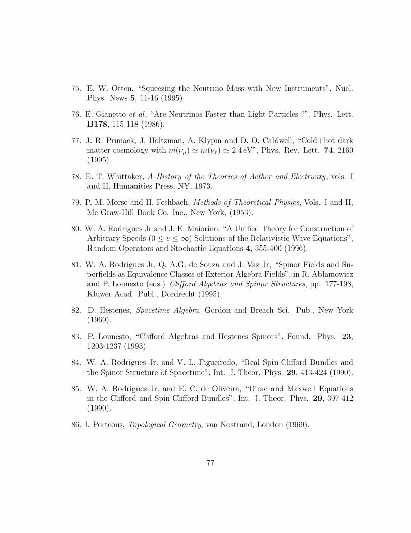
75. E. W. Otten, “Squeezing the Neutrino Mass with New Instruments”, Nucl.Phys. News 5, 11-16 (1995).

76. E. Gianetto et al , “Are Neutrinos Faster than Light Particles ?”, Phys. Lett.B178, 115-118 (1986).

77. J. R. Primack, J. Holtzman, A. Klypin and D. O. Caldwell, “Cold+hot darkmatter cosmology with m(νµ) ≃ m(ντ ) ≃ 2.4 eV”, Phys. Rev. Lett. 74, 2160(1995).

78. E. T. Whittaker, A History of the Theories of Aether and Electricity , vols. Iand II, Humanities Press, NY, 1973.

79. P. M. Morse and H. Feshbach, Methods of Theoretical Physics, Vols. I and II,Mc Graw-Hill Book Co. Inc., New York, (1953).

80. W. A. Rodrigues Jr and J. E. Maiorino, “A Unified Theory for Construction ofArbitrary Speeds (0 ≤ v ≤ ∞) Solutions of the Relativistic Wave Equations”,Random Operators and Stochastic Equations 4, 355-400 (1996).

81. W. A. Rodrigues Jr, Q. A.G. de Souza and J. Vaz Jr, “Spinor Fields and Su-perfields as Equivalence Classes of Exterior Algebra Fields”, in R. Ablamowiczand P. Lounesto (eds.) Clifford Algebras and Spinor Structures, pp. 177-198,Kluwer Acad. Publ., Dordrecht (1995).

82. D. Hestenes, Spacetime Algebra, Gordon and Breach Sci. Pub., New York(1969).

83. P. Lounesto, “Clifford Algebras and Hestenes Spinors”, Found. Phys. 23,1203-1237 (1993).

84. W. A. Rodrigues Jr. and V. L. Figueiredo, “Real Spin-Clifford Bundles andthe Spinor Structure of Spacetime”, Int. J. Theor. Phys. 29, 413-424 (1990).

85. W. A. Rodrigues Jr. and E. C. de Oliveira, “Dirac and Maxwell Equationsin the Clifford and Spin-Clifford Bundles”, Int. J. Theor. Phys. 29, 397-412(1990).

86. I. Porteous, Topological Geometry, van Nostrand, London (1969).

77

arX

iv:h

ep-t

h/96

0617

1 v4

16

Oct

199

7

Polynomial WaveformSynthesizer

(Model Data 2045)

A/DConverter

50 dB ENI rfPower Amplifier

(Model 240L)

Transducer

WaterWater Tank

Scan Hydrophone

Stepping Motor

LinearAmplifier

1 V DCOffsetBuffer

MC 68000Computer

Stepping MotorDriver

TapeDriver

HardDisk

DataMonitor

ConsoleTerminal

Transformer(Impedance: 16:1)

05/91/JYL

TRIG

arXiv:hep-th/9606171 v4 16 Oct 1997

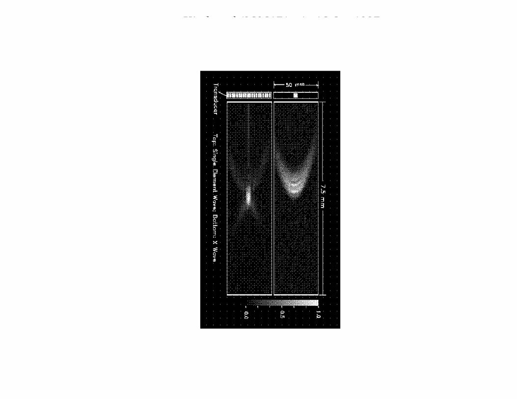
arXiv:hep-th/9606171 v4 16 Oct 1997

arXiv:hep-th/9606171 v4 16 Oct 1997

arXiv:hep-th/9606171 v4 16 Oct 1997

arXiv:hep-th/9606171 v4 16 Oct 1997

arXiv:hep-th/9606171 v4 16 Oct 1997

arXiv:hep-th/9606171 v4 16 Oct 1997

arXiv:hep-th/9606171 v4 16 Oct 1997