NBER WORKING PAPER SERIES

THE WAGE STRUCTURE AND THE SORTING OF WORKERSINTO THE PUBLIC SECTOR

George J. Borjas

Working Paper 9313http://www.nber.org/papers/w9313

NATIONAL BUREAU OF ECONOMIC RESEARCH1050 Massachusetts Avenue

Cambridge, MA 02138October 2002

The views expressed herein are those of the authors and not necessarily those of the National Bureau ofEconomic Research.

© 2002 by George J. Borjas. All rights reserved. Short sections of text, not to exceed two paragraphs, maybe quoted without explicit permission provided that full credit, including © notice, is given to the source.

The Wage Structure and the Sorting of Workers into the Public SectorNBER Working Paper No. 9313October 2002JEL No. J3, J4

ABSTRACTThis paper uses data from the U.S. Decennial Census and the Current Population Surveys to

document the differential shifts that occurred in the wage structures of the public and privatesectorsbetween 1960 and 2000. The wage gap between the typical public sector worker and a comparable privatesector worker was relatively constant for men during this period, but declined substantially for women.Equally important, wage dispersion in the public sector was increasing relative to wage dispersion in theprivate sector prior to 1970, at the time when public sector employment was rising rapidly. Since 1970,however, there has been a significant relative compression of the wage distribution in the public sector.The different evolutions of the wage structures in the two sectors are an important determinant of thesorting of workers across sectors. As a result of the relative wage compression, the public sector foundit increasingly more difficult to attract and retain high-skill workers.

George J. BorjasKennedy School of GovernmentHarvard University79 JFK StreetCambridge, MA 02138and NBERgborjas@harvard.edu

2

THE WAGE STRUCTURE AND THE SORTING OF WORKERS INTO THE PUBLIC SECTOR

George J. Borjas*

The public sector employs around 16 percent of the American workforce. Since the

1970s, there has been a flurry of research activity attempting to document and understand the pay

practices of that sector. Smith (1977), for instance, began a voluminous empirical literature that

examines if public sector workers receive “equal pay for equal work” when compared to their

private sector counterparts (see also Gyourko and Tracy, 1988; Moulton, 1990; and Katz and

Krueger, 1991).1

The last two decades have also witnessed a remarkable change in the U.S. wage structure.

In particular, there has been a substantial increase in wage inequality among salaried workers,

both between and within skill groups.2 There is little disagreement that such an increase

occurred. There is still a debate, however, over the factors that may have caused the widening of

the wage distribution.3 The “list of usual suspects” includes the de-unionization of the U.S. labor

market, the increased globalization of the economy, the resurgence of immigration, and skill-

biased technological change.

* Robert W. Scrivner Professor of Economics and Social Policy, John F. Kennedy School of Government,

Harvard University; and Research Associate, National Bureau of Economic Research.

1 There have also been many studies that analyze various aspects of the labor market in the public sector, such as the interplay between political factors and market forces in setting public sector pay (Borjas, 1980, 1984; Craig, 1995); employment discrimination and comparable worth remedies (Borjas, 1982; Hundley, 1993); the determination of job queues and quit rates (Black, Moffitt, and Warner, 1990; Ippolito, 1987; Krueger, 1988); and wage-setting in particular local governments or federal agencies (Moore and Newman, 1991; Perloff and Wachter, 1984). Ehrenberg and Schwarz (1986) and Gregory and Borland (1999) provide detailed surveys of this literature.

2 Juhn, Murphy, and Pierce (1993), Katz and Murphy (1992), and Murphy and Welch (1992) document these important trends.

3 Studies identifying some of the factors responsible for the changes in the wage structure include Bound and Johnson (1992), Freeman (1993), and Autor, Katz, and Krueger (1998). Katz and Autor (1999) present a detailed survey of the literature.

3

Although much of the focus in the debate over the public sector wage structure has

emphasized the size of the pay differential between the typical worker employed in the public

sector and a statistically comparable counterpart in the private sector, this emphasis is somewhat

myopic. Given the remarkable changes in the wage structure that occurred over the past 20 years,

it is unlikely that the wage structure evolved in similar ways in the private and public sectors. As

a result, there could be sizable differences in the trend of the public-private sector pay gap for

workers in different skill groups.

Differential changes in the wage structure between the public and private sectors can be

reasonably expected to alter the behavior of many economic agents. Suppose (as is actually the

case) that wage dispersion has been rising at a faster rate in private sector jobs than in public

sector jobs. The relative change in the wage structure would then suggest that private sector

workers who belong to highly skilled groups (such as college graduates), or private sector

workers who have relatively high earnings within a particular skill group, will have reduced

incentives to enter the public sector. Conversely, public sector workers who belong to highly

skilled groups, or public sector workers who have relatively high incomes within a particular

skill group, will have increased incentives to leave the public sector and enter private sector jobs.

In short, the relative changes in the wage structure should influence labor supply decisions, and

alter the sorting of workers between the two sectors.

This paper uses data drawn from the U.S. decennial Censuses and from the Current

Population Surveys (CPS) to document the changes in the wage structure that occurred in the

private and public sectors between 1960 and 2000.4 The evidence suggests that relative wage

4 The paper is closely related to the analysis of Katz and Krueger (1991), who also use CPS data between

1967 and 1987 to estimate both the size of the pay gap between public and private sector workers, as well as to provide some evidence on the different evolutions of the wage structure in the two sectors. The present paper updates many of the Katz-Krueger calculations through the year 2000, as well as extends the analysis by

4

inequality was actually rising in the public sector prior to 1970, but that there has been

substantial relative wage compression in that sector since the 1970s. The paper also examines if

the different evolution of the wage structure in the two sectors altered the behavioral decision of

how workers allocate themselves between the sectors. The empirical analysis suggests that as a

result of the relative compression of public-sector wages since 1970, high-skill private sector

workers became increasingly less likely to quit their jobs to enter the public sector, and high-skill

public sector workers became increasingly more likely to switch to the private sector.

Trends in Employment and Pay Levels

It is instructive to begin the discussion by describing some general trends in public sector

employment and pay over the past few decades. I will use two main sources of data throughout

much of the study: a 1 percent sample drawn from the Public Use Microdata Samples (PUMS) of

the U.S. Census for the years 1960 through 1990; and the Annual Demographic Supplement (i.e.,

the March Supplement) of the Current Population Surveys for the years 1977 through 2001.

I restrict the analysis to workers who are between 18 and 64 years old and are not self-

employed. A particular worker is classified as employed in the private or public sectors based on

the information provided in the “class of work” variable in these data sets. This variable indicates

if the worker is employed in the public or private sector. Beginning with the 1970 Census, the

class of work variable also indicates if a public sector worker is employed by the federal, state,

or local governments.

investigating the link between the skills of workers who move across sectors and the relative changes in the wage structures.

5

Employment

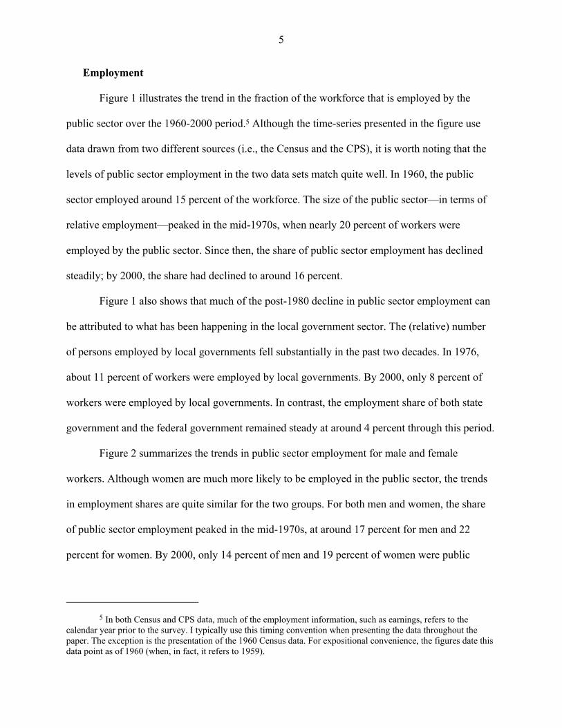
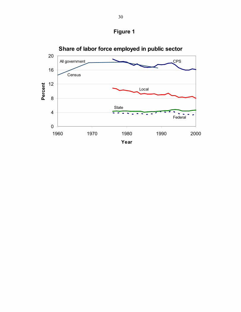
Figure 1 illustrates the trend in the fraction of the workforce that is employed by the

public sector over the 1960-2000 period.5 Although the time-series presented in the figure use

data drawn from two different sources (i.e., the Census and the CPS), it is worth noting that the

levels of public sector employment in the two data sets match quite well. In 1960, the public

sector employed around 15 percent of the workforce. The size of the public sector—in terms of

relative employment—peaked in the mid-1970s, when nearly 20 percent of workers were

employed by the public sector. Since then, the share of public sector employment has declined

steadily; by 2000, the share had declined to around 16 percent.

Figure 1 also shows that much of the post-1980 decline in public sector employment can

be attributed to what has been happening in the local government sector. The (relative) number

of persons employed by local governments fell substantially in the past two decades. In 1976,

about 11 percent of workers were employed by local governments. By 2000, only 8 percent of

workers were employed by local governments. In contrast, the employment share of both state

government and the federal government remained steady at around 4 percent through this period.

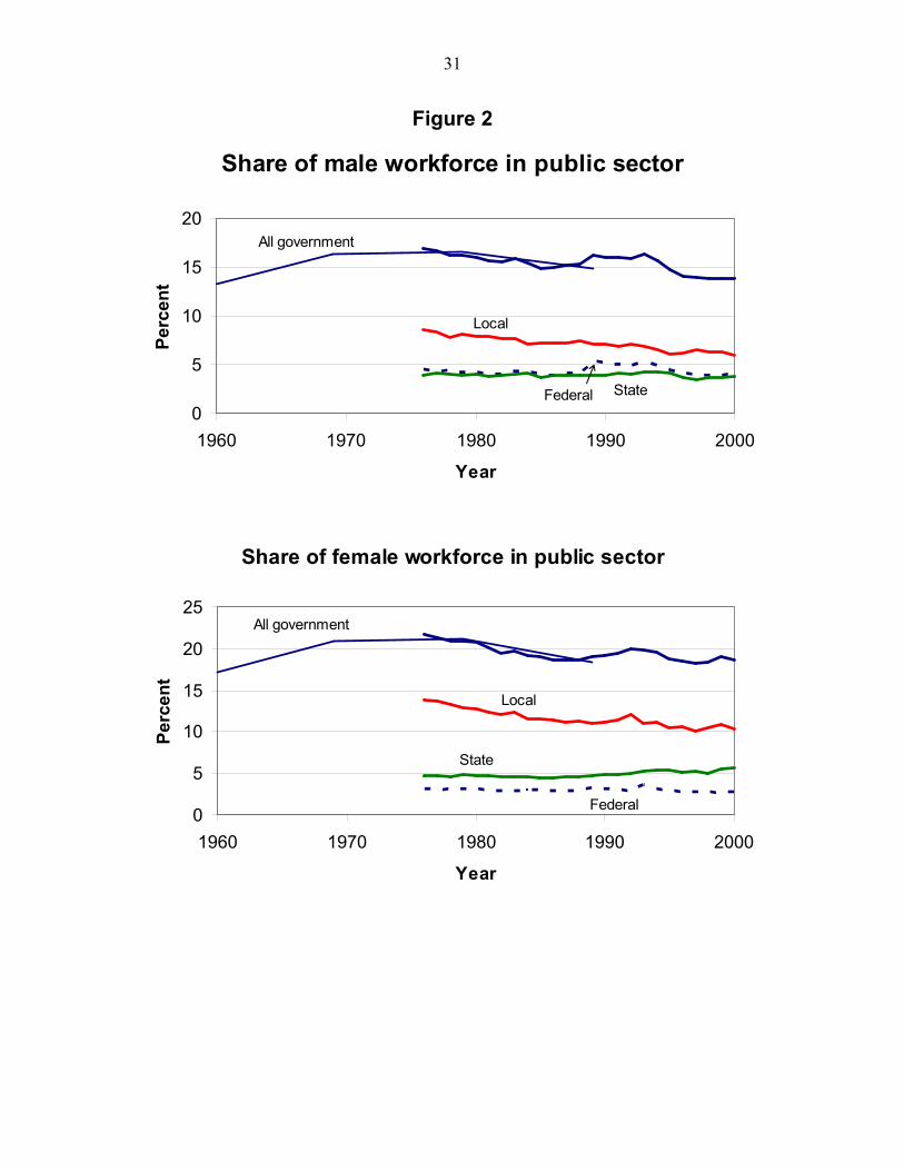
Figure 2 summarizes the trends in public sector employment for male and female

workers. Although women are much more likely to be employed in the public sector, the trends

in employment shares are quite similar for the two groups. For both men and women, the share

of public sector employment peaked in the mid-1970s, at around 17 percent for men and 22

percent for women. By 2000, only 14 percent of men and 19 percent of women were public

5 In both Census and CPS data, much of the employment information, such as earnings, refers to the

calendar year prior to the survey. I typically use this timing convention when presenting the data throughout the paper. The exception is the presentation of the 1960 Census data. For expositional convenience, the figures date this data point as of 1960 (when, in fact, it refers to 1959).

6

sector employees, and much of the decline in employment for both men and women can be

attributed to the contracting size of the local government sector.

The public sector pay gap

Many studies calculate the pay gap between comparable workers in the public and private

sectors, and examine variations in this pay gap over time and across the various levels of

government. In this section, I update this large literature by documenting the long-run trends in

the pay gap between 1960 and 2000.

To calculate the wage differential between public and private sector workers, I use the

sample restrictions typically used in the studies that document the evolution of the wage structure

in the wage-and-salary sector (Katz and Autor, 1999). In particular, I restrict the analysis to the

sample to full-time workers (persons who worked at least 40 weeks per year and 35 hours per

week in the calendar year prior to the survey). In addition, I restrict the sample to those full-time

workers who earned at least $67 per week in 1982 dollars (implying that their hourly income was

at least half of the 1982 real minimum wage). Throughout the analysis, I will use the log of

weekly wages as the dependent variable. Because there is a substantial wage differential between

men and women—both in the public and private sectors—I will estimate the public sector pay

gap separately for each gender. Initially, I focus on measuring the pay gap between the

(aggregate) public and private sectors. I will discuss the pay differences that exist among the

federal, state, and local government sectors below.

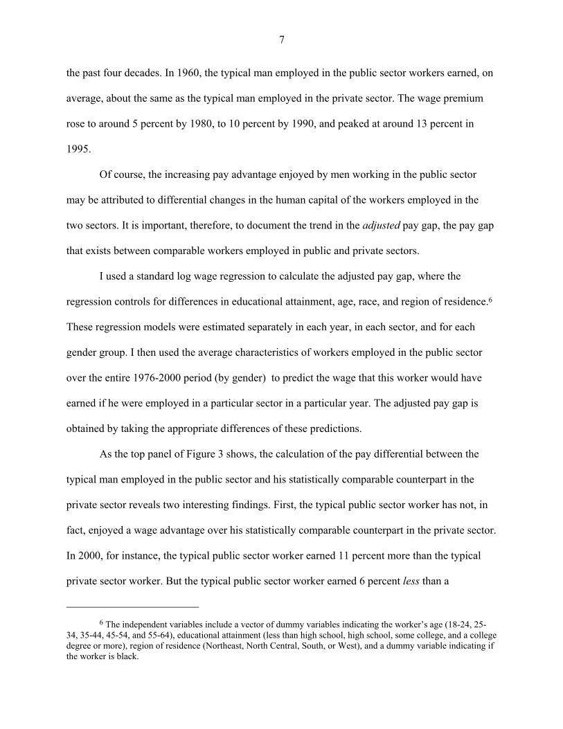
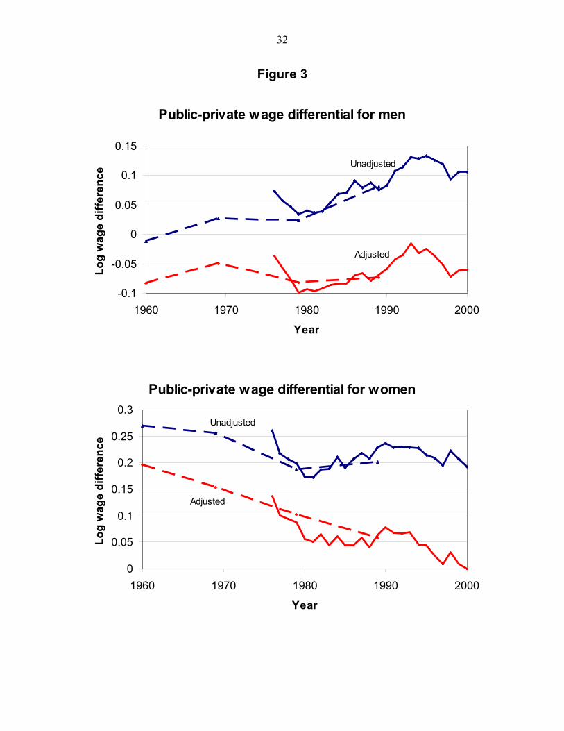
The top panel of Figure 3 illustrates the trend in the (unadjusted) log wage differential

between the typical male public sector worker and the typical male private sector worker. It is

evident that the wage advantage enjoyed by men employed in the public sector rose steadily over

7

the past four decades. In 1960, the typical man employed in the public sector workers earned, on

average, about the same as the typical man employed in the private sector. The wage premium

rose to around 5 percent by 1980, to 10 percent by 1990, and peaked at around 13 percent in

1995.

Of course, the increasing pay advantage enjoyed by men working in the public sector

may be attributed to differential changes in the human capital of the workers employed in the

two sectors. It is important, therefore, to document the trend in the adjusted pay gap, the pay gap

that exists between comparable workers employed in public and private sectors.

I used a standard log wage regression to calculate the adjusted pay gap, where the

regression controls for differences in educational attainment, age, race, and region of residence.6

These regression models were estimated separately in each year, in each sector, and for each

gender group. I then used the average characteristics of workers employed in the public sector

over the entire 1976-2000 period (by gender) to predict the wage that this worker would have

earned if he were employed in a particular sector in a particular year. The adjusted pay gap is

obtained by taking the appropriate differences of these predictions.

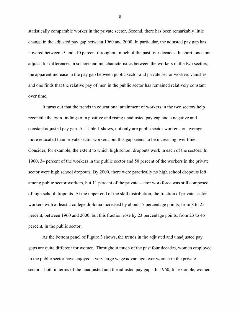
As the top panel of Figure 3 shows, the calculation of the pay differential between the

typical man employed in the public sector and his statistically comparable counterpart in the

private sector reveals two interesting findings. First, the typical public sector worker has not, in

fact, enjoyed a wage advantage over his statistically comparable counterpart in the private sector.

In 2000, for instance, the typical public sector worker earned 11 percent more than the typical

private sector worker. But the typical public sector worker earned 6 percent less than a

6 The independent variables include a vector of dummy variables indicating the worker’s age (18-24, 25-

34, 35-44, 45-54, and 55-64), educational attainment (less than high school, high school, some college, and a college degree or more), region of residence (Northeast, North Central, South, or West), and a dummy variable indicating if the worker is black.

8

statistically comparable worker in the private sector. Second, there has been remarkably little

change in the adjusted pay gap between 1960 and 2000. In particular, the adjusted pay gap has

hovered between -5 and -10 percent throughout much of the past four decades. In short, once one

adjusts for differences in socioeconomic characteristics between the workers in the two sectors,

the apparent increase in the pay gap between public sector and private sector workers vanishes,

and one finds that the relative pay of men in the public sector has remained relatively constant

over time.

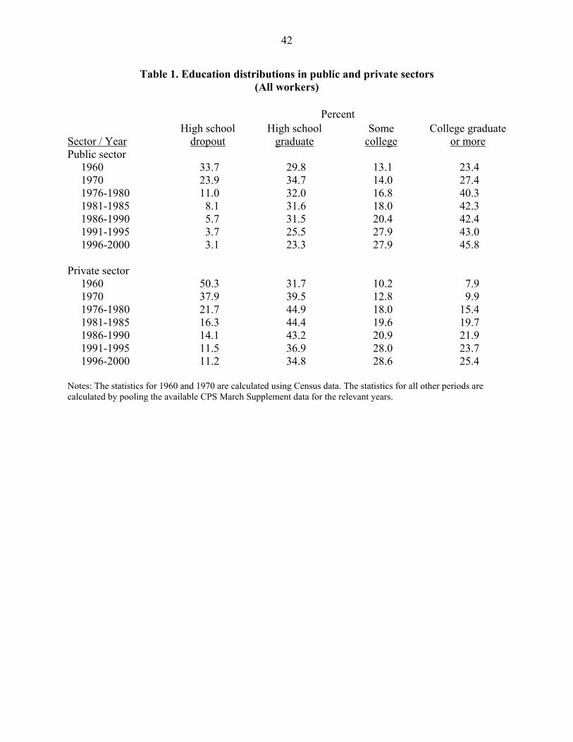
It turns out that the trends in educational attainment of workers in the two sectors help

reconcile the twin findings of a positive and rising unadjusted pay gap and a negative and

constant adjusted pay gap. As Table 1 shows, not only are public sector workers, on average,

more educated than private sector workers, but this gap seems to be increasing over time.

Consider, for example, the extent to which high school dropouts work in each of the sectors. In

1960, 34 percent of the workers in the public sector and 50 percent of the workers in the private

sector were high school dropouts. By 2000, there were practically no high school dropouts left

among public sector workers, but 11 percent of the private sector workforce was still composed

of high school dropouts. At the upper end of the skill distribution, the fraction of private sector

workers with at least a college diploma increased by about 17 percentage points, from 8 to 25

percent, between 1960 and 2000, but this fraction rose by 23 percentage points, from 23 to 46

percent, in the public sector.

As the bottom panel of Figure 3 shows, the trends in the adjusted and unadjusted pay

gaps are quite different for women. Throughout much of the past four decades, women employed

in the public sector have enjoyed a very large wage advantage over women in the private

sector—both in terms of the unadjusted and the adjusted pay gaps. In 1960, for example, women

9

in the public sector earned around 27 percent more than women in the private sector, and the pay

gap remained at 20 percent even after adjusting for differences in socioeconomic characteristics

between female workers in the two sectors. By 2000, the unadjusted pay gap had fallen slightly

to around 20 percent. However, the monetary advantage suggested by the adjusted pay gap had

completely disappeared, so that the typical woman employed in the public sector earned just as

much as her statistically comparable counterpart in the private sector. This decline in the pay

advantage of women employed in the public sector partly reflects the significant improvement in

economic opportunities that private sector female workers experienced over the past few

decades.

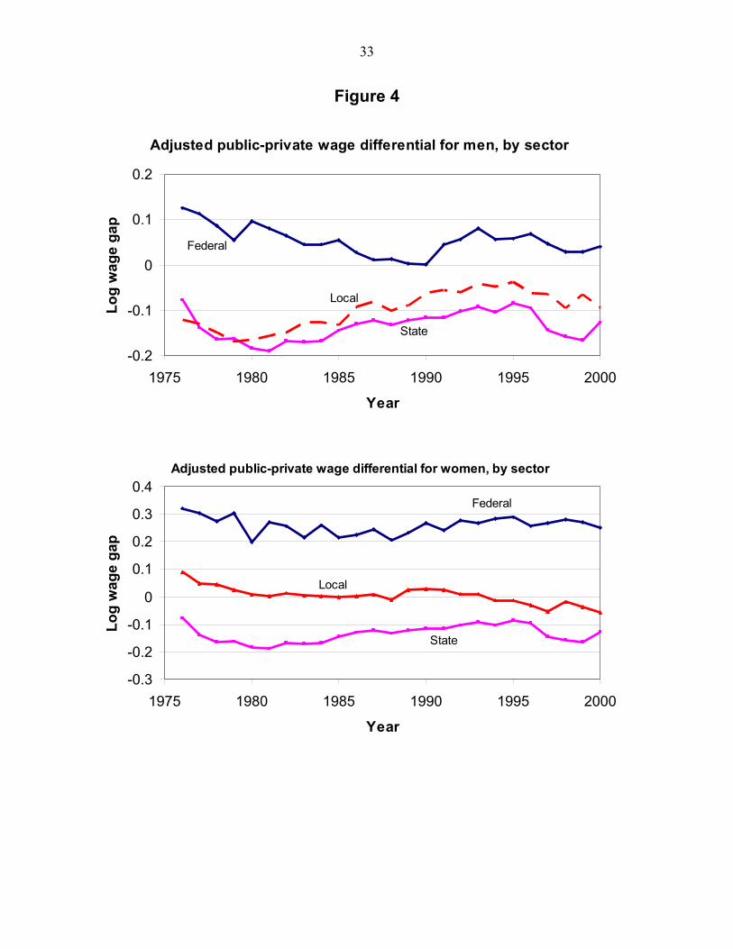
The two panels of Figure 4 show the different trends in the adjusted pay gap (between the

public and private sector) across the various government sectors. It turns out that the aggregate

trends illustrated in the previous figures mask a great deal of variation in pay levels among the

federal, state, and local government sectors. In particular, Figure 4 shows that, regardless of

gender, workers in the federal sector enjoy a significant pay premium over comparable workers

in the private sector, while workers employed by state governments suffer a significant wage

disadvantage.

For men, the adjusted pay gap between the federal and private sectors declined

somewhat, from over 10 percent in the mid-1970s to around 3 percent by 2000. At the same

time, however, men employed in state and local governments experienced some improvement in

their pay status. In 1980, these men had wage penalties of around 15 to 20 percent, but the size of

the penalty fell to around 10 percent by 2000.

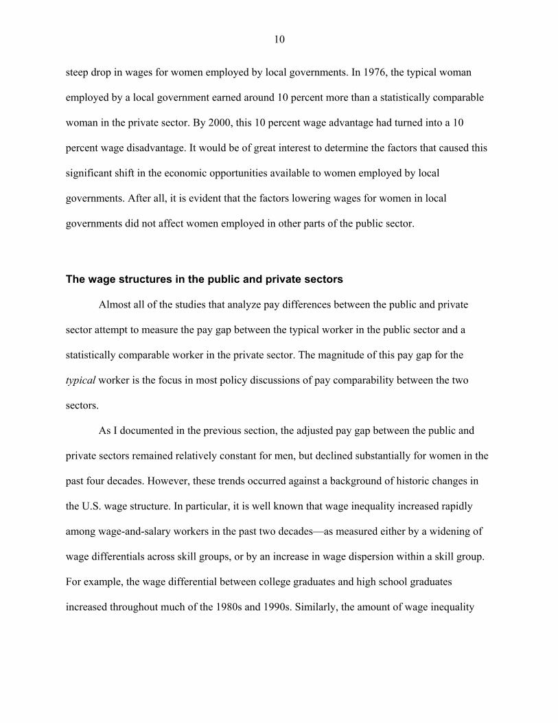
It turns out that the significant decline in the adjusted wage premium accruing to the

typical woman employed in the public sector (and documented in Figure 3) can be attributed to a

10

steep drop in wages for women employed by local governments. In 1976, the typical woman

employed by a local government earned around 10 percent more than a statistically comparable

woman in the private sector. By 2000, this 10 percent wage advantage had turned into a 10

percent wage disadvantage. It would be of great interest to determine the factors that caused this

significant shift in the economic opportunities available to women employed by local

governments. After all, it is evident that the factors lowering wages for women in local

governments did not affect women employed in other parts of the public sector.

The wage structures in the public and private sectors

Almost all of the studies that analyze pay differences between the public and private

sector attempt to measure the pay gap between the typical worker in the public sector and a

statistically comparable worker in the private sector. The magnitude of this pay gap for the

typical worker is the focus in most policy discussions of pay comparability between the two

sectors.

As I documented in the previous section, the adjusted pay gap between the public and

private sectors remained relatively constant for men, but declined substantially for women in the

past four decades. However, these trends occurred against a background of historic changes in

the U.S. wage structure. In particular, it is well known that wage inequality increased rapidly

among wage-and-salary workers in the past two decades—as measured either by a widening of

wage differentials across skill groups, or by an increase in wage dispersion within a skill group.

For example, the wage differential between college graduates and high school graduates

increased throughout much of the 1980s and 1990s. Similarly, the amount of wage inequality

11

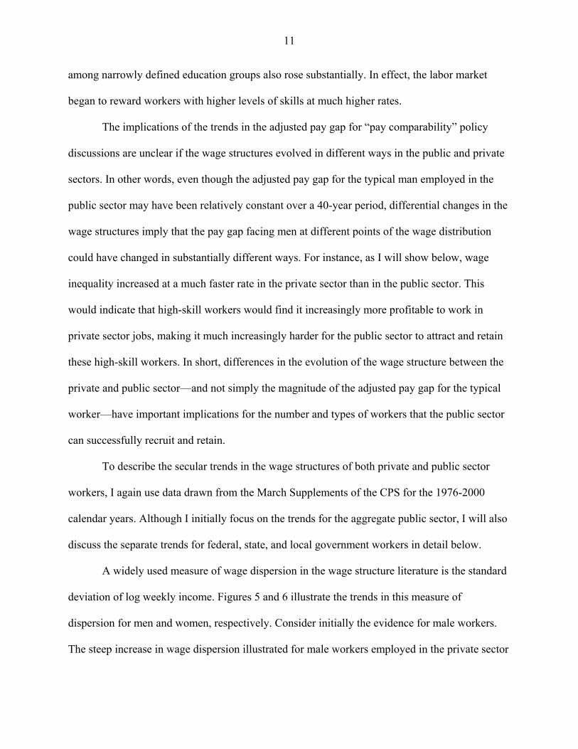
among narrowly defined education groups also rose substantially. In effect, the labor market

began to reward workers with higher levels of skills at much higher rates.

The implications of the trends in the adjusted pay gap for “pay comparability” policy

discussions are unclear if the wage structures evolved in different ways in the public and private

sectors. In other words, even though the adjusted pay gap for the typical man employed in the

public sector may have been relatively constant over a 40-year period, differential changes in the

wage structures imply that the pay gap facing men at different points of the wage distribution

could have changed in substantially different ways. For instance, as I will show below, wage

inequality increased at a much faster rate in the private sector than in the public sector. This

would indicate that high-skill workers would find it increasingly more profitable to work in

private sector jobs, making it much increasingly harder for the public sector to attract and retain

these high-skill workers. In short, differences in the evolution of the wage structure between the

private and public sector—and not simply the magnitude of the adjusted pay gap for the typical

worker—have important implications for the number and types of workers that the public sector

can successfully recruit and retain.

To describe the secular trends in the wage structures of both private and public sector

workers, I again use data drawn from the March Supplements of the CPS for the 1976-2000

calendar years. Although I initially focus on the trends for the aggregate public sector, I will also

discuss the separate trends for federal, state, and local government workers in detail below.

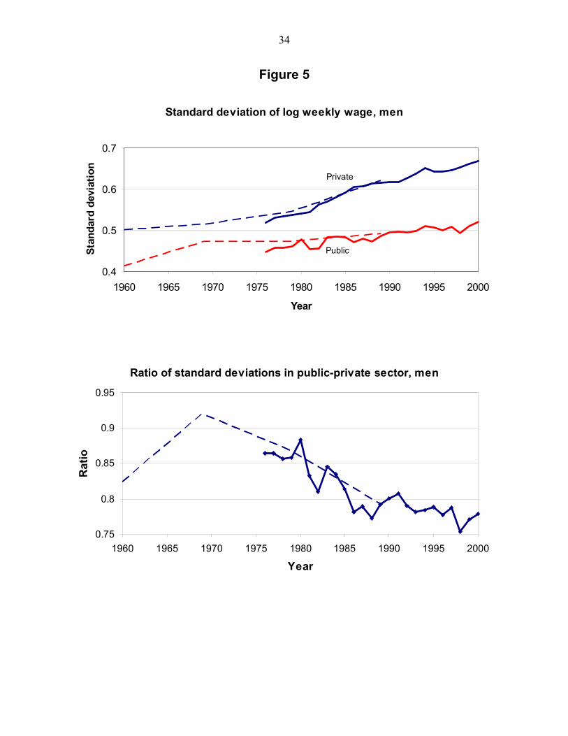
A widely used measure of wage dispersion in the wage structure literature is the standard

deviation of log weekly income. Figures 5 and 6 illustrate the trends in this measure of

dispersion for men and women, respectively. Consider initially the evidence for male workers.

The steep increase in wage dispersion illustrated for male workers employed in the private sector

12

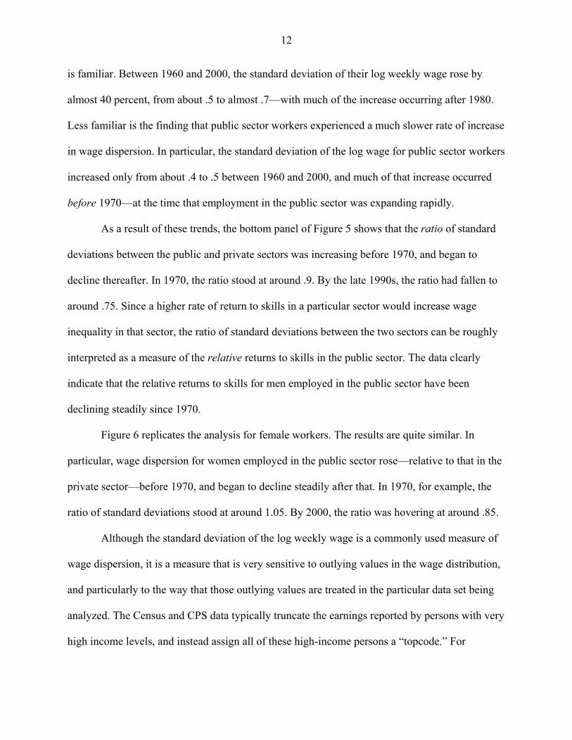
is familiar. Between 1960 and 2000, the standard deviation of their log weekly wage rose by

almost 40 percent, from about .5 to almost .7—with much of the increase occurring after 1980.

Less familiar is the finding that public sector workers experienced a much slower rate of increase

in wage dispersion. In particular, the standard deviation of the log wage for public sector workers

increased only from about .4 to .5 between 1960 and 2000, and much of that increase occurred

before 1970—at the time that employment in the public sector was expanding rapidly.

As a result of these trends, the bottom panel of Figure 5 shows that the ratio of standard

deviations between the public and private sectors was increasing before 1970, and began to

decline thereafter. In 1970, the ratio stood at around .9. By the late 1990s, the ratio had fallen to

around .75. Since a higher rate of return to skills in a particular sector would increase wage

inequality in that sector, the ratio of standard deviations between the two sectors can be roughly

interpreted as a measure of the relative returns to skills in the public sector. The data clearly

indicate that the relative returns to skills for men employed in the public sector have been

declining steadily since 1970.

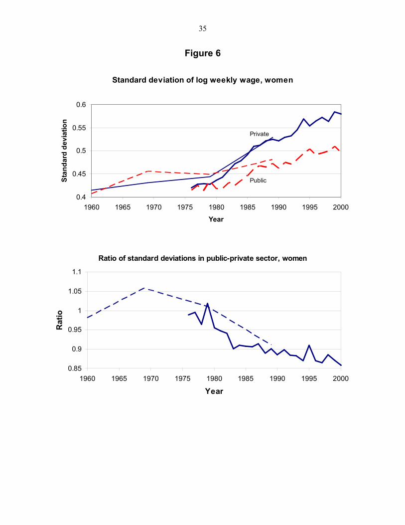
Figure 6 replicates the analysis for female workers. The results are quite similar. In

particular, wage dispersion for women employed in the public sector rose—relative to that in the

private sector—before 1970, and began to decline steadily after that. In 1970, for example, the

ratio of standard deviations stood at around 1.05. By 2000, the ratio was hovering at around .85.

Although the standard deviation of the log weekly wage is a commonly used measure of

wage dispersion, it is a measure that is very sensitive to outlying values in the wage distribution,

and particularly to the way that those outlying values are treated in the particular data set being

analyzed. The Census and CPS data typically truncate the earnings reported by persons with very

high income levels, and instead assign all of these high-income persons a “topcode.” For

13

example, all persons who earned more than $75,000 in the 1980 Census are coded as imply

earning $75,000. To make matters worse, the truncation point for nominal earnings changes in a

haphazard way over time. As a result, the differential topcoding of earnings in different periods

can influence the relative trend in the standard deviation of log weekly earnings, particularly if

workers in one sector are more likely to be topcoded than workers in another sector.7

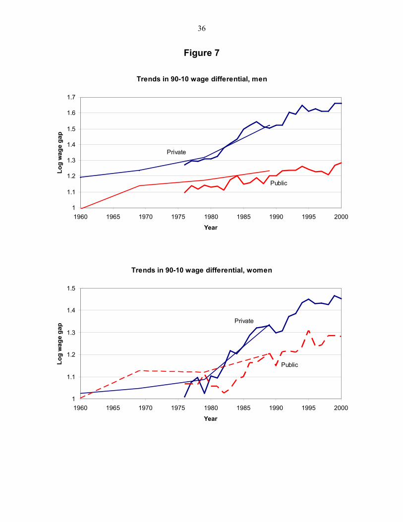
One can avoid this technical problem by using an alternative measure of wage dispersion,

such as the wage gap between the workers at the 90th percentile and the 10th percentile of the

wage distribution. This measure of wage dispersion, which I will call the “90-10 wage gap,”

essentially discards the earnings information for the topcoded observations, and is obviously not

sensitive to the technical problems introduced by the topcoding of observations.

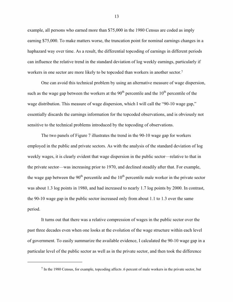
The two panels of Figure 7 illustrates the trend in the 90-10 wage gap for workers

employed in the public and private sectors. As with the analysis of the standard deviation of log

weekly wages, it is clearly evident that wage dispersion in the public sector—relative to that in

the private sector—was increasing prior to 1970, and declined steadily after that. For example,

the wage gap between the 90th percentile and the 10th percentile male worker in the private sector

was about 1.3 log points in 1980, and had increased to nearly 1.7 log points by 2000. In contrast,

the 90-10 wage gap in the public sector increased only from about 1.1 to 1.3 over the same

period.

It turns out that there was a relative compression of wages in the public sector over the

past three decades even when one looks at the evolution of the wage structure within each level

of government. To easily summarize the available evidence, I calculated the 90-10 wage gap in a

particular level of the public sector as well as in the private sector, and then took the difference

7 In the 1980 Census, for example, topcoding affects .6 percent of male workers in the private sector, but

14

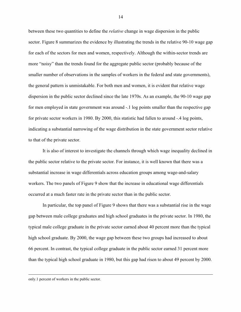
between these two quantities to define the relative change in wage dispersion in the public

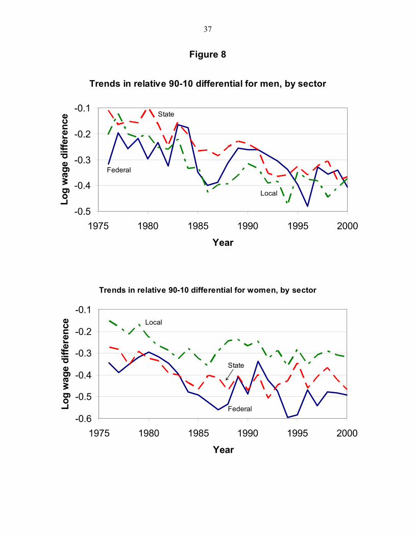
sector. Figure 8 summarizes the evidence by illustrating the trends in the relative 90-10 wage gap

for each of the sectors for men and women, respectively. Although the within-sector trends are

more “noisy” than the trends found for the aggregate public sector (probably because of the

smaller number of observations in the samples of workers in the federal and state governments),

the general pattern is unmistakable. For both men and women, it is evident that relative wage

dispersion in the public sector declined since the late 1970s. As an example, the 90-10 wage gap

for men employed in state government was around -.1 log points smaller than the respective gap

for private sector workers in 1980. By 2000, this statistic had fallen to around -.4 log points,

indicating a substantial narrowing of the wage distribution in the state government sector relative

to that of the private sector.

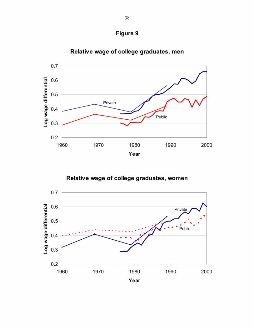
It is also of interest to investigate the channels through which wage inequality declined in

the public sector relative to the private sector. For instance, it is well known that there was a

substantial increase in wage differentials across education groups among wage-and-salary

workers. The two panels of Figure 9 show that the increase in educational wage differentials

occurred at a much faster rate in the private sector than in the public sector.

In particular, the top panel of Figure 9 shows that there was a substantial rise in the wage

gap between male college graduates and high school graduates in the private sector. In 1980, the

typical male college graduate in the private sector earned about 40 percent more than the typical

high school graduate. By 2000, the wage gap between these two groups had increased to about

66 percent. In contrast, the typical college graduate in the public sector earned 31 percent more

than the typical high school graduate in 1980, but this gap had risen to about 49 percent by 2000.

only.1 percent of workers in the public sector.

15

The bottom panel of Figure 9 shows a similar widening of educational wage differentials for

women in the private sector, and a much smaller widening in the public sector. In fact, the wage

gap between college graduates and high school graduates used to be larger in the public sector

than in the private sector in 1980. In particular, this educational wage gap was 37 percent in the

public sector and 34 percent in the private sector. By 2000, the wage gap between college

graduates and high school graduates had risen to 60 percent in the private sector, and to only 53

percent in the public sector. In sum, part of the relative compression of the wage distribution in

the public sector can be directly attributed to the fact that the increase in the returns to schooling

in public sector jobs did not keep pace with the rise observed in the private sector during the

1980s and 1990s.

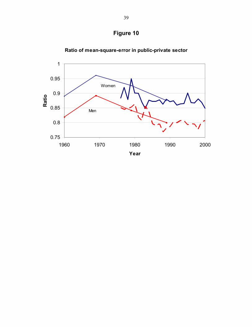
Finally, it is also the case that wage inequality in the private sector rose relative to wage

inequality in the public sector even within narrowly defined skill groups. I measure within-group

wage inequality by the mean-square-error (i.e., the standard deviation of the residual) from a

regression of log weekly earnings on age, schooling, region of residence, and race. This

regression was estimated separately for each sector, for each gender group, and in each calendar

year. Figure 10 illustrates the trend in the ratio of the within-group adjusted standard deviations

of the log weekly wage between the public and private sectors. The figure clearly shows that

within-group relative inequality was rising in the public sector prior to 1970, and has fallen

steadily since.8

In sum, the analysis of the Census and CPS data available since 1960 clearly indicate that

there has been a substantial difference in how the wage structures of the public and private

8 To conserve space, I do not show the trends in the educational wage gap or the mean-square-error for the

federal, state, and local government sectors separately. Though noisier, the trends within each of the sectors resemble the aggregate trend that indicates a relative compression in government wages both across and within skill groups.

16

sectors evolved during this period. The much-documented increase in wage inequality, both

across and within skill groups, is most evident among private sector workers. Income inequality,

either across or within skill groups, did not rise as much in the public sector. Interestingly, this

trend was not always the case. Prior to the 1970s, at the time that public sector employment was

expanding rapidly, wage inequality was, in fact, rising at a much faster rate in the public sector

than in the private sector.

The Sorting of Workers between Sectors

The fact that relative wages across and within skill groups changed at very different rates

in the public and private sectors during the 1980s and 1990s implies that the economic incentives

that induce particular types of persons to enter or leave a particular sector also changed over the

period.9 For instance, suppose the same types of workers tend to do well in both public and

private sector jobs—assuming, in effect, that there is a strong positive correlation in potential

earnings across the two sectors. Private sector workers who belong to the high-skill groups, or

who do quite well within a particular skill groups, should now have fewer incentives to enter

public sector jobs. Similarly, public sector workers who belong to the high-skill groups, or who

do quite well within a particular skill group, should now have greater incentives to quit their

public sector jobs and enter the private sector. In short, the relative compression of wages in the

public sector should alter the sorting of workers between the two sectors. Over time, the public

sector should find it increasingly more difficult to attract high-skill workers from their current

private sector positions, and to prevent high-skill workers from quitting and moving on to the

private sector.

9 Blank (1985) presents an early analysis of how workers choose between the public and private sectors.

17

One can measure how these incentive effects influence the allocation of workers by

analyzing the movement of workers between the private and public sectors, and by examining

how the skill composition of this flow responded to the relative compression of wages in the

public sector. In particular, consider two specific groups of workers. The first group is composed

of workers who are initially employed in private sector firms, and who over some time period

enter the public sector. The second group is composed of workers who are initially in the public

sector, but who decide to leave those jobs and enter the private sector.

Of course, the creation of samples representing these groups of “movers” requires that

workers be observed over time, so that we can observe their decision to switch sectors. I conduct

the analysis of these in-transit workers by using data drawn from the 1979-2001 CPS Outgoing

Rotation Group files (CPS-ORG), which have the key advantage that they provide a much larger

sample of workers than the March Supplements of the CPS.10 Some of the workers in these files

can be matched across two consecutive calendar years. These matched data can be used to

determine if the person’s class of work (i.e., public or private sector) changed between the two-

year period. As before, I restrict the analysis to wage-and-salary workers aged 18 to 64.

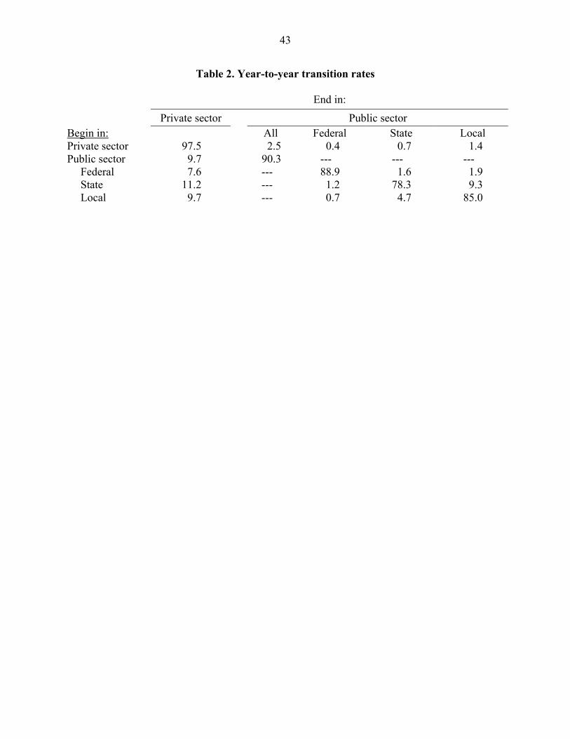
Table 2 summarizes the transition rates between the various sectors for the entire 1979-

2001 sample period.11 During this period, the year-to-year transition rate from the private sector

10 The Current Population Surveys uses a particular type of sample rotation to interview persons. In

particular, a chosen household is in the CPS for four months in a row, is then dropped from the sample for 8 months, and is then re-interviewed for four more months. The questionnaire given to the outgoing rotation group (i.e., in the fourth and sixteenth months) contains detailed questions about income and other labor force characteristics. Each annual CPS-ORG file contains about 100,000 working men aged 18-64, so they are significantly larger than the March samples. Due to changes in the survey design, workers cannot be matched between 1984 and 1985, or between 1994 and 1995. For reasons that are not well documented, it is also very difficult to match workers between the 1995 and 1996 surveys. One drawback with the CPS-ORG is that its income data differs from the income data reported in the more commonly used March files. In particular, instead of reporting the annual income in the year prior to the survey, the data reports usual monthly income.

11 The transition rates are calculated in the sample of workers who worked in both years, so that they do not capture transitions in and out of the labor force.

18

to the public sector was only 2.5 percent, with most of these movers obtaining a job in the local

sector. In contrast, the mobility rate from the public sector to the private sector was 9.7 percent.

The transition rate out of the public sector varies significantly across the various levels of

government: it was 7.6 percent for federal workers, 11.2 percent for state workers, and 9.7

percent for local government workers. The data also reveal a significant amount of mobility

between the state and local sectors, but relatively little movement between the federal sector and

other levels of government. In particular, nearly 9.3 percent of state government workers moved

to a local government job, and 4.7 percent of local government workers moved to a state job. In

contrast, only 1.2 percent of state government workers and 0.7 percent of local government

workers moved to a federal job.

For most of what follows, I focus on transitions between the public and private sectors,

and ignore those transitions that occur within the public sector itself. Define the quit rate from

public sector jobs as the fraction of workers who were initially employed in the public sector, but

who became private sector workers in the following year. Similarly, define the entry rate into the

public sector as the fraction of workers who were initially in the private sector, and who moved

to a public sector job in the following year.

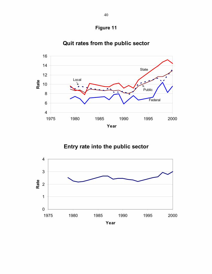
The top panel of Figure 11 illustrates the year-to-year quit rates out of the public sector. It

is evident that there was a significant increase in the quit rate out of the public sector beginning

around 1990. In the late 1980s, for example, the quit rate out of public sector jobs was just below

9 percent. By 2000, this quit rate had increased to almost 13 percent. Moreover, it is evident that

there has been a significant increase in quit rates for all levels of government. In the federal

sector, for instance, the quit rate rose from 5.8 to 9.6 percent between 1990 and 2000, while in

the local sector the increase was from 8.5 to 13.2 percent. The bottom of Figure 11 illustrates the

19

trend in year-to-year entry rates into the public sector. Not surprisingly, since these entry rates

are mainly determined by employment demand in the public sector, the entry rates are much

more stable over time, hovering between 2 and 3 percent throughout the entire period.

As noted above, the characteristics of the workers who entered—or who left—the public

sector in the past two decades should have changed in response to the relative changes in the

wage structure. I now turn to a more formal analysis of this hypothesis.

To simplify the analysis, I restrict the study to the sample of “marginal” workers—that is,

those workers who either left or entered the public sector during any two-year period. The

empirical analysis, therefore, ignores the largest group of workers, those who did not change

sectors. This group of non-movers either did not pay attention to the changing opportunities

provided by the different evolution of wage structures, or found that, perhaps because of the high

transaction costs involved in any move, they could not fully take advantage of the changing

opportunities and were “stuck” in their initial placement. By focusing on the sample of movers,

the analysis should be able to isolate the impact of the relative compression of wages in the

public sector on the sorting of workers across sectors, if any such impact actually exists.

Before proceeding to a more formal study of the impact of the wage structure on the

sorting mechanism, it is instructive to examine, at a purely descriptive level, how the average

quality of the marginal workers changed during the period under study. To conduct this type of

empirical analysis, it is crucial to judiciously match workers across the available CPS-ORG

surveys. In particular, consider the workers who are employed in the private sector in some

calendar year t. By linking these workers in the CPS-ORG data across years t and t+1, I can

observe the private sector earnings of workers who are about to enter the public sector. Similarly,

by linking workers across years t-1 and t, I can observe the private sector earnings of workers

20

who have just left the public sector. In short, in any given CPS-ORG cross-section I can measure

the private sector earnings of two distinct groups of workers: workers who are about to enter the

public sector and workers who have just left the public sector. The comparison of the private

sector earnings of these two groups—and how the wage difference between these groups varies

as the public sector wage structure became relatively more compressed—should provide a great

deal of information about the impact of the changing wage structures on the sorting of workers

across the two sectors.12

To easily show the correlation between the quit decision and worker quality, consider the

quit behavior exhibited by workers in different parts of the wage distribution. Given my

definition of the “marginal” worker—as workers who are either leaving or entering the private

sector—I can use the private sector wage distribution in each calendar year to rank all workers in

the data. I can then calculate the quit rate out of the public sector for workers in each tercile of

the wage distribution. Figure 12 shows the trend in the quit rates for the top tercile relative to the

other groups. It is evident that the quit behavior of workers in the top third of the distribution

differs substantially from that of workers in the other deciles. In particular, high-skill workers

have much lower quit rates, but the quit rate for these high-skill workers rose at a much faster

rate during the 1980s and 1990s—at the same time that the relative pay for these types of

workers was improving substantially in the private sector.13

12 Ideally, one would want to define three distinct samples of private sector workers in year t by merging

the relevant CPS files for calendar years t-1, t, and t+1: those workers who are in the private sector in all three years, those who just entered the private sector, and those who are about to leave the private sector. It would be of great interest to estimate the relative wages of the three groups. Unfortunately, the survey design of the CPS does not allow such an exercise since no person can appear in more than two consecutive years of the data. I can obtain the sample of quitters and entrants, but cannot isolate the workers who stayed in the private sector throughout. This data constraint helps further explain why I focus on analyzing the relative wage of the two groups of marginal workers.

13 The trend for the relative entry rate of high-skill workers is less insightful because it is mainly driven by the increasing demand of the public sector for high-skill workers.

21

To summarize, the judicious merging of CPS-ORG data across years isolates two distinct

groups of “marginal” workers who are in the private sector in any given calendar year. The first

are workers who have just entered the private sector, and the second are workers who are about

to leave the private sector. The comparison of the skills of these two groups of marginal workers

should help indicate how the differential changes in the two structures affects the sorting of

workers across sectors. In particular, consider the regression model to be estimated in the pooled

sample of these marginal workers:

(1) log wit = Xit b0t + α Qit + β σt + γ (Qit × σt) + εit,

where wit gives the weekly wage of private-sector worker i at time t; X is a vector of

socioeconomic characteristics (described below); Qit is a dummy variable set to unity if the

worker has just quit the public sector, and set to zero if the worker is about to enter the public

sector; and σ is a measure of the relative dispersion in the public sector at time t.14 For

simplicity, I use the sex-specific ratio of standard deviations between the public and private

sectors as the measure of dispersion. Since the wage structure evolved somewhat differently for

male and female workers, the variable σt takes on a different value for men and women at any

given point in time. The parameter of interest in this regression model is the coefficient γ, which

indicates how the wage differential between workers who have just quit the public sector and

workers who are about to enter the public sector varies with respect to the relative dispersion in

14 The regression model also includes a vector of dummy variables indicating if the “marginal” worker is in

the federal sector, the state sector, or the local sector. In addition, the regression includes a measure of the public-private sector wage differential, which clearly can affect the number of workers who move across sectors, and thereby intensify or dilute the selection effect. The inclusion of these variables in the regression model does not alter the qualitative implications of the results reported below.

22

the public sector. I have argued that the wage differential between the “quitters” and the

“entrants” should be larger when there is more compression in the public sector (i.e., the quitters

will tend to be high-skill workers, and high-skill workers will not want to enter the public

sector). The coefficient γ, therefore, should be negative.

I estimated this regression model on the sample drawn from the CPS-ORG data by

pooling all of the marginal workers over all the years for which the merging could be conducted.

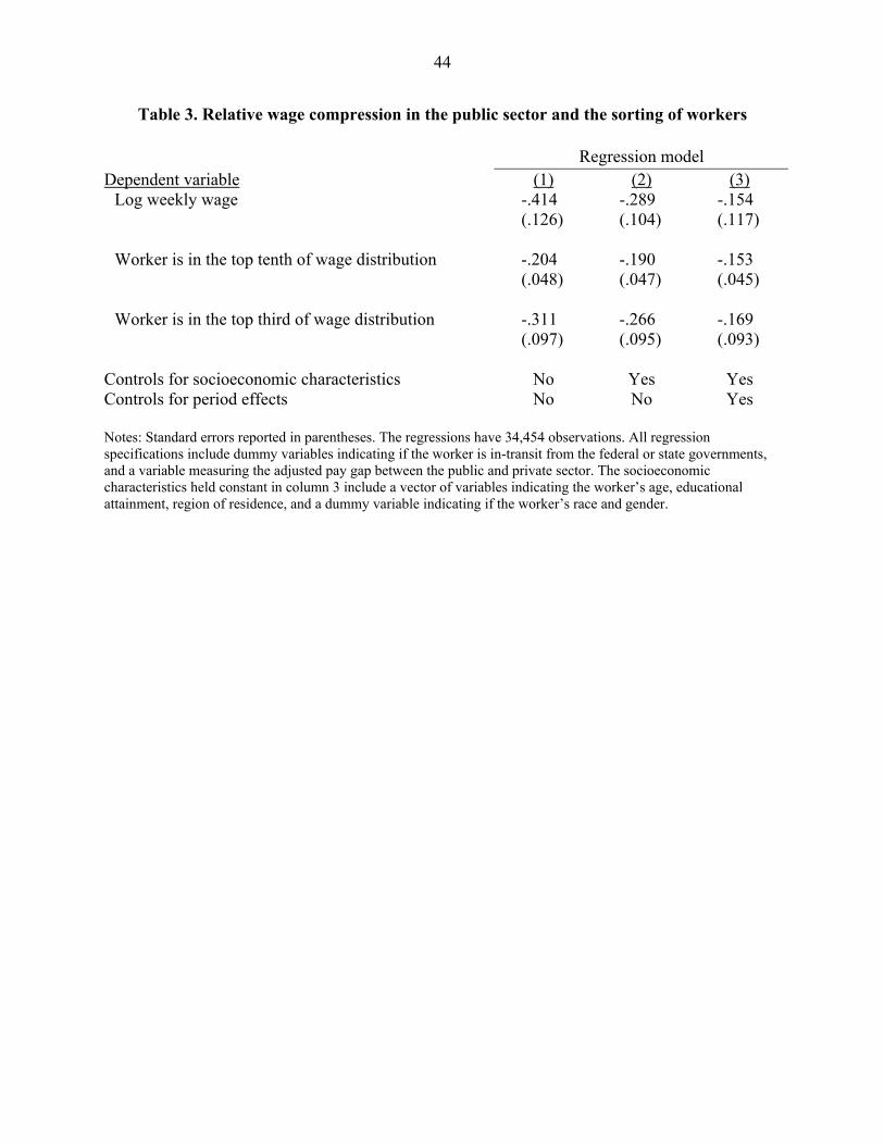
Table 3 presents the estimates of the coefficient γ. Consider the first row of the table, which

corresponds to the regression model specified in equation (1). In the absence of any variables

standardizing for differences in observable skills across workers, the first column of the table

reports a statistically significant estimate of -.414 for the coefficient γ.

It is instructive to interpret this coefficient in terms of a specific simulation of the model.

In particular, I documented earlier (see Figures 5 and 6) that the relative ratio of standard

deviations between the public and private sectors declined by about .15 percentage points

between 1976 and 1990. One can use the estimated coefficient of -.414 to predict the impact of

this observed decline in relative wage dispersion on the wage differential between the workers

who have just quit the public sector and workers who are about to enter the public sector. In

particular, the relative compression of the public sector wage distribution increased the wage

differential between quitters and entrants by 6 percentage points (or -.414 times -.15). It is

evident, therefore, that the impact of the wage structure on the relative quality of workers that the

public sector attracts and retains is not only statistically significant, but numerically important.

The other columns of the first row of Table 3 investigate the nature of this sorting effect

in more detail. The second column addresses the possibility that the variable measuring the

relative dispersion in the public sector wage structure is just “standing in” for a time trend. As I

23

showed earlier, relative dispersion in the public sector declined steadily since 1970. It may well

be that for some unrelated reason the wage gap between the quitters and the entrants was rising

over time, and the regression coefficient γ is just capturing a spurious correlation. To net out this

spurious effect, I add a vector of dummy variables indicating the calendar year in which the

observation is observed to the regression model. This vector is not completely collinear with the

relative dispersion variable (σt) because the dispersion variable takes on different values for men

and women. By including these period effects, the coefficient γ now measures the impact of

relative dispersion on the wage gap between quitters and entrants in any particular year. It is

evident that the estimated effect remains negative and significant. In fact, the estimated

coefficient of -.289 implies that the .15 percentage point drop in the relative dispersion of the

public sector wage distribution increased the wage gap between those who have just quit the

public sector and those who are about to enter it by about 4 percent points.

The last column of the table introduces a number of standardizing variables in the

regression model, including the age, race, educational attainment, and region of residence of the

worker. Even after adjusting for differences in these variables across workers, as well as for

period effects, the data reveal a link between the sorting of workers and the wage structure

(although the coefficient is not significant). There is a possibility, however, that the regression is

“over-controlling” by including these socioeconomic characteristics. After all, the different

evolutions of the wage structures in the two sectors will lead different types of workers (such as

more educated workers) to choose different sectors.

The remaining rows of the table look at alternative measures of the impact of relative

wage compression on worker quality. Instead of using the log weekly wage as the dependent

variable in the regression model, the dependent variable in the second row indicates if the worker

24

is in the top tenth of the private sector wage distribution. The coefficient γ now measures the

difference in the probability of being in the top tenth of the distribution between quitters and

entrants. Finally, the dependent variable in the third row is the probability that the worker is in

the top third of the wage distribution.

Table 3 clearly shows that there are significant sorting effects when worker quality is

defined in terms of worker placement in the private sector wage distribution. Consider, for

example, the difference in the probability that quitters and entrants are in the top third of the

wage distribution. This difference is very sensitive to the relative compression of wages in the

public sector. In particular, the .15 percentage point decline in the relative dispersion of the

public sector implies about a 5 percentage point increase in the difference between the

probability that a quitter and an entrant are in the top third of the wage distribution. In short, the

relative compression of wages in the public sector significantly altered the incentives of persons

in the upper tail of the wage distribution to consider jobs in the public sector.

The sorting evidence presented in Table 3 aggregates all the levels of government into a

single group, the public sector, and netted out any sectoral effects on the wage gap between

quitters and entrants by including dummy variables indicating if the marginal worker was in the

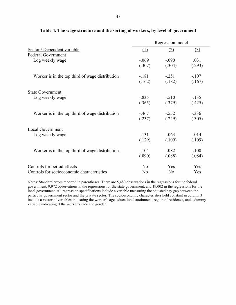
federal, state, or local governments. Table 4 reports the results when the regression model is

estimated separately for the marginal workers in each sector of government.15 Each of the three

samples being considered, therefore, contains workers who either have just quit or are about to

enter a particular level of government (e.g., the state government). The relative dispersion

variable (σt) is now defined in terms of the ratio of standard deviations between the particular

government sector and the private sector. Since the measure of within-sector relative dispersion

25

is noisier because of the smaller samples, it is not surprising that the standard errors of the

estimated sorting effect tend to be higher than in the analysis that pooled observations across

government sectors. Nevertheless, the data are roughly consistent with the hypothesis that the

relative compression of wages in each of the levels of government in the public sector adversely

affected the quality of the workforce in that sector.

In the state government sector, for example, the relative measure of dispersion dropped

by .1 percentage points between 1976 and 2000. The estimate of the coefficient γ in Table 4 (in

the absence of any controlling variables) is -.835. This coefficient implies that the observed

compression of wages in the state government sector (relative to the private sector) generated an

8 percentage point increase in the wage gap between workers who have just left the state

government sector and workers who are about to enter it, an effect that is both numerically and

statistically significant. The evidence tends to be weakest for federal workers, where most of the

estimated coefficients are negative, but not statistically significant.

Summary

This paper documents that the wage distributions in the public and private sectors

evolved in different ways in the past four decades. In general terms, the public-private sector pay

gap between the typical public sector worker and a comparable private sector worker was

relatively constant for men between 1960 and 2000, but declined substantially for women.

Equally important, prior to 1970, at the time when public sector employment was rising rapidly,

wage dispersion in the public sector was increasing relative to wage dispersion in the private

15 The measure of relative dispersion used in the regression models is the measure of compression that

applies to the particular sector (i.e. federal, state, or local government).

26

sector. Beginning in the 1970s, however, this situation reversed, and there has been a significant

relative compression of the wage distribution in the public sector during the past two decades.

The differential shifts in the wage structures of the two sectors will likely affect labor

supply behavior by altering the sorting of workers between the sectors. As long as the correlation

between economic performance in the public and private sectors is strong and positive (so that

the same persons tend to be relatively successful regardless of where they work), these labor

supply responses suggest that high-skill workers will increasingly want to be employed in the

private sector.

This paper used data drawn from the Current Population Surveys to investigate if such a

supply response occurred. The evidence suggests that as the wage structures evolved, the relative

skills of the “marginal” persons who moved across sectors also changed significantly. For

example, the wage differential between persons who had just quit the public sector and workers

who were about to enter that sector is strongly and negatively correlated with the relative

dispersion of incomes in the public sector. Put differently, as the wage structure in the public

sector became relatively more compressed, the public sector found it harder to attract and retain

high-skill workers. In short, the substantial widening of wage inequality in the private sector and

the relatively more stable wage distribution in the public sector created “magnetic effects” that

altered the sorting of workers across sectors, with high-skill workers becoming more likely to

end up in the private sector.

Although most studies of pay determination in the public sector focus on the earnings gap

between the typical worker in the public sector and his statistical counterpart in the private

sector, it is clear that the difference in the shape of the wage distributions between the two

sectors plays a significant role in determining the public sector’s ability to attract and retain a

27

high-quality workforce. The analysis suggests that future policy discussions of public sector

wages need to pay a great deal more attention to the relative dispersion in the income

opportunities offered to government workers.

28

REFERENCES Autor, David H., Lawrence F. Katz, and Alan B. Krueger. “Computing Inequality: Have Computers Changed the Labor Market?” Quarterly Journal of Economics, Vol. 113, No. 4 (November 1988): 1169-1213.

Black, Matthew; Robert Moffitt, and John. T. Warner. “The Dynamics of Job Separation: The Case of Federal Employees,” Journal of Applied Econometrics, Vol. 5, No. 3. (July-August 1990): 245-262.

Blank, Rebecca M. “An Analysis of Workers' Choice between Employment in the Public and Private Sectors,” Industrial and Labor Relations Review, Vol. 38, No. 2. (January 1985): 211-224.

Borjas, George J. “Wage Determination in the Federal Government: The Role of Constituents and Bureaucrats,” Journal of Political Economy Vol. 88, No. 6 (December 1980): 1110-1147.

Borjas, George J. “The Politics of Employment Discrimination in the Federal

Bureaucracy,” Journal of Law and Economics, Vol. 25, No. 2 (October 1982): 271-299.

Borjas, George J. “Electoral Cycles and the Earnings of Federal Bureaucrats,” Economic Inquiry, Vol. 22, No. 4 (October 1984): 447-459. Bound, John and George Johnson. “Changes in the Structure of Wages in the 1980s: An Evaluation of Alternative Explanations,” American Economic Review, Vol. 82, No. 3 (June 1992): 371-392.

Craig, Lee A. “The Political Economy of Public-Private Compensation Differentials: The Case of Federal Pensions,” Journal of Economic History, Vol. 55, No. 2. (June 1995): 304-320. Ehrenberg, Ronald G. and Joshua L. Schwarz. “Public Sector Labor Markets,” in Orley Ashenfelter and Richard Layard, editors, Handbook of Labor Economics, Vol. 2. Amsterdam: North-Holland, 1986: 1219-1268. Freeman, Richard B. “How Much Has De-Unionization Contributed to the Rise in Male Earnings Inequality,” in Sheldon Danzinger and Peter Gottschalk, editors, Uneven Tides: Rising Inequality in America. New York: Russell Sage Foundation, 1993: 133-163. Gregory, Robert G. and Jeff Borland. “Recent Developments in Public Sector Labor Markets,” in Orley Ashenfelter and David Card, eds., Handbook of Labor Economics, Volume 3C. Amsterdam: North-Holland, 1999: 3573-3630. Gyourko, Joseph and Joseph Tracy. “An Analysis of Public- and Private-Sector Wages Allowing for Endogenous Choices of Both Government and Union Status,” Journal of Labor Economics, Vol. 6, No. 2. (April 1988): 229-253.

29

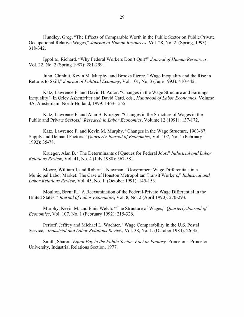
Hundley, Greg, “The Effects of Comparable Worth in the Public Sector on Public/Private

Occupational Relative Wages,” Journal of Human Resources, Vol. 28, No. 2. (Spring, 1993): 318-342. Ippolito, Richard. “Why Federal Workers Don’t Quit?” Journal of Human Resources, Vol. 22, No. 2 (Spring 1987): 281-299. Juhn, Chinhui, Kevin M. Murphy, and Brooks Pierce. “Wage Inequality and the Rise in Returns to Skill,” Journal of Political Economy, Vol. 101, No. 3 (June 1993): 410-442. Katz, Lawrence F. and David H. Autor. “Changes in the Wage Structure and Earnings Inequality.” In Orley Ashenfelter and David Card, eds., Handbook of Labor Economics, Volume 3A. Amsterdam: North-Holland, 1999: 1463-1555. Katz, Lawrence F. and Alan B. Krueger. “Changes in the Structure of Wages in the Public and Private Sectors,” Research in Labor Economics, Volume 12 (1991): 137-172. Katz, Lawrence F. and Kevin M. Murphy. “Changes in the Wage Structure, 1963-87: Supply and Demand Factors,” Quarterly Journal of Economics, Vol. 107, No. 1 (February 1992): 35-78. Krueger, Alan B. “The Determinants of Queues for Federal Jobs,” Industrial and Labor Relations Review, Vol. 41, No. 4 (July 1988): 567-581.

Moore, William J. and Robert J. Newman. “Government Wage Differentials in a Municipal Labor Market: The Case of Houston Metropolitan Transit Workers,” Industrial and Labor Relations Review, Vol. 45, No. 1. (October 1991): 145-153. Moulton, Brent R. “A Reexamination of the Federal-Private Wage Differential in the United States,” Journal of Labor Economics, Vol. 8, No. 2 (April 1990): 270-293. Murphy, Kevin M. and Finis Welch. “The Structure of Wages,” Quarterly Journal of Economics, Vol. 107, No. 1 (February 1992): 215-326.

Perloff, Jeffrey and Michael L. Wachter. “Wage Comparability in the U.S. Postal Service,” Industrial and Labor Relations Review, Vol. 38, No. 1. (October 1984): 26-35. Smith, Sharon. Equal Pay in the Public Sector: Fact or Fantasy. Princeton: Princeton University, Industrial Relations Section, 1977.

30

Figure 1

Share of labor force employed in public sector

0

4

8

12

16

20

1960 1970 1980 1990 2000

Year

Perc

ent

All government

Census

CPS

Local

State

Federal

31

Figure 2

Share of male workforce in public sector

0

5

10

15

20

1960 1970 1980 1990 2000

Year

Perc

ent

All government

Local

StateFederal

Share of female workforce in public sector

0

5

10

15

20

25

1960 1970 1980 1990 2000

Year

Perc

ent

All government

Local

State

Federal

32

Figure 3

Public-private wage differential for men

-0.1

-0.05

0

0.05

0.1

0.15

1960 1970 1980 1990 2000

Year

Log

wag

e di

ffere

nce Unadjusted

Adjusted

Public-private wage differential for women

0

0.05

0.1

0.15

0.2

0.25

0.3

1960 1970 1980 1990 2000

Year

Log

wag

e di

ffere

nce

Unadjusted

Adjusted

33

Figure 4

Adjusted public-private wage differential for men, by sector

-0.2

-0.1

0

0.1

0.2

1975 1980 1985 1990 1995 2000

Year

Log

wag

e ga

p

Federal

Local

State

Adjusted public-private wage differential for women, by sector

-0.3

-0.2

-0.1

0

0.1

0.2

0.3

0.4

1975 1980 1985 1990 1995 2000

Year

Log

wag

e ga

p

Federal

Local

State

34

Figure 5

Standard deviation of log weekly wage, men

0.4

0.5

0.6

0.7

1960 1965 1970 1975 1980 1985 1990 1995 2000

Year

Stan

dard

dev

iatio

n

Private

Public

Ratio of standard deviations in public-private sector, men

0.75

0.8

0.85

0.9

0.95

1960 1965 1970 1975 1980 1985 1990 1995 2000

Year

Rat

io

35

Figure 6

Standard deviation of log weekly wage, women

0.4

0.45

0.5

0.55

0.6

1960 1965 1970 1975 1980 1985 1990 1995 2000

Year

Stan

dard

dev

iatio

n

Private

Public

Ratio of standard deviations in public-private sector, women

0.85

0.9

0.95

1

1.05

1.1

1960 1965 1970 1975 1980 1985 1990 1995 2000

Year

Rat

io

36

Figure 7

Trends in 90-10 wage differential, men

1

1.1

1.2

1.3

1.4

1.5

1.6

1.7

1960 1965 1970 1975 1980 1985 1990 1995 2000

Year

Log

wag

e ga

p

Private

Public

Trends in 90-10 wage differential, women

1

1.1

1.2

1.3

1.4

1.5

1960 1965 1970 1975 1980 1985 1990 1995 2000

Year

Log

wag

e ga

p Private

Public

37

Figure 8

Trends in relative 90-10 differential for men, by sector

-0.5

-0.4

-0.3

-0.2

-0.1

1975 1980 1985 1990 1995 2000

Year

Log

wag

e di

ffere

nce

Federal

State

Local

Trends in relative 90-10 differential for women, by sector

-0.6

-0.5

-0.4

-0.3

-0.2

-0.1

1975 1980 1985 1990 1995 2000

Year

Log

wag

e di

ffere

nce

Federal

State

Local

38

Figure 9

Relative wage of college graduates, men

0.2

0.3

0.4

0.5

0.6

0.7

1960 1970 1980 1990 2000

Year

Log

wag

e di

ffere

ntia

l

Public

Private

Relative wage of college graduates, women

0.2

0.3

0.4

0.5

0.6

0.7

1960 1970 1980 1990 2000

Year

Log

wag

e di

ffere

ntia

l

Public

Private

39

Figure 10

Ratio of mean-square-error in public-private sector

0.75

0.8

0.85

0.9

0.95

1

1960 1970 1980 1990 2000

Year

Rat

io

Women

Men

40

Figure 11

Quit rates from the public sector

4

6

8

10

12

14

16

1975 1980 1985 1990 1995 2000

Year

Rat

e

Federal

State

Public

Local

Entry rate into the public sector

0

1

2

3

4

1975 1980 1985 1990 1995 2000

Year

Rat

e

41

Figure 12

Relative quit rates of high-skill workers

0.2

0.3

0.4

0.5

0.6

0.7

0.8

0.9

1

1975 1980 1985 1990 1995 2000

Year

Rat

io

Top tercile relative to bottom tercile

Top tercile relative to middle tercile

42

Table 1. Education distributions in public and private sectors (All workers)

Percent Sector / Year

High school dropout

High school graduate

Some college

College graduate or more

Public sector 1960 33.7 29.8 13.1 23.4 1970 23.9 34.7 14.0 27.4 1976-1980 11.0 32.0 16.8 40.3 1981-1985 8.1 31.6 18.0 42.3 1986-1990 5.7 31.5 20.4 42.4 1991-1995 3.7 25.5 27.9 43.0 1996-2000 3.1 23.3 27.9 45.8

Private sector

1960 50.3 31.7 10.2 7.9 1970 37.9 39.5 12.8 9.9 1976-1980 21.7 44.9 18.0 15.4 1981-1985 16.3 44.4 19.6 19.7 1986-1990 14.1 43.2 20.9 21.9 1991-1995 11.5 36.9 28.0 23.7 1996-2000 11.2 34.8 28.6 25.4

Notes: The statistics for 1960 and 1970 are calculated using Census data. The statistics for all other periods are calculated by pooling the available CPS March Supplement data for the relevant years.

43

Table 2. Year-to-year transition rates End in:

Private sector Public sector Begin in: All Federal State Local Private sector 97.5 2.5 0.4 0.7 1.4 Public sector 9.7 90.3 --- --- ---

Federal 7.6 --- 88.9 1.6 1.9 State 11.2 --- 1.2 78.3 9.3 Local 9.7 --- 0.7 4.7 85.0

44

Table 3. Relative wage compression in the public sector and the sorting of workers Regression model Dependent variable (1) (2) (3)

Log weekly wage -.414 -.289 -.154 (.126) (.104) (.117) Worker is in the top tenth of wage distribution -.204 -.190 -.153 (.048) (.047) (.045) Worker is in the top third of wage distribution -.311 -.266 -.169

(.097) (.095) (.093) Controls for socioeconomic characteristics No Yes Yes Controls for period effects No No Yes Notes: Standard errors reported in parentheses. The regressions have 34,454 observations. All regression specifications include dummy variables indicating if the worker is in-transit from the federal or state governments, and a variable measuring the adjusted pay gap between the public and private sector. The socioeconomic characteristics held constant in column 3 include a vector of variables indicating the worker’s age, educational attainment, region of residence, and a dummy variable indicating if the worker’s race and gender.

45

Table 4. The wage structure and the sorting of workers, by level of government Regression model Sector / Dependent variable (1) (2) (3) Federal Government

Log weekly wage -.069 -.090 .031 (.307) (.304) (.293) Worker is in the top third of wage distribution -.181 -.251 -.107 (.162) (.182) (.167)

State Government

Log weekly wage -.835 -.510 -.135 (.365) (.379) (.425) Worker is in the top third of wage distribution -.467 -.552 -.336

(.237) (.249) (.305) Local Government

Log weekly wage -.131 -.063 .014 (.129) (.109) (.109) Worker is in the top third of wage distribution -.104 -.082 -.100

(.090) (.088) (.084)

Controls for period effects No Yes Yes Controls for socioeconomic characteristics No No Yes Notes: Standard errors reported in parentheses. There are 5,480 observations in the regressions for the federal government, 9,972 observations in the regressions for the state government, and 19,002 in the regressions for the local government. All regression specifications include a variable measuring the adjusted pay gap between the particular government sector and the private sector. The socioeconomic characteristics held constant in column 3 include a vector of variables indicating the worker’s age, educational attainment, region of residence, and a dummy variable indicating if the worker’s race and gender.