WACC parameter estimates for Essential Energy - … - WACC... · Final ii Table of Contents 1...
41
Final i WACC parameter estimates for Essential Energy Dr. Tom Hird November 2017
Transcript of WACC parameter estimates for Essential Energy - … - WACC... · Final ii Table of Contents 1...

Final i
WACC parameter estimates for Essential Energy
Dr. Tom Hird
November 2017

Final ii
Table of Contents
1 Executive summary 1
1.1 Estimating the cost of debt 1
1.2 Estimating the cost of equity 3
1.3 WACC estimates 4
2 Introduction 7
2.1 Report structure 7
3 Best estimate of cost of debt 8
3.1 Best estimate of cost of debt 8
3.2 Debt term 9
3.3 Debt management strategy 9
3.4 Base rate 13
3.5 Spread 14
3.6 Alternative cost of debt estimates 22
4 Best estimate of cost of equity 25
4.1 Risk-free rate 25
4.2 Equity beta 25
4.3 Cost of equity estimates 33
5 Conclusion on WACC estimates 35

Final iii
List of Figures
Figure 1-1: Difference in cost of debt compared to best estimate (%) .................................. 3
Figure 3-1: Reproduction of Figure 9 from May 2014 report - RBA, CBASpectrum
and Bloomberg ................................................................................................... 19
Figure 3-2: BVAL curves at different maturities .................................................................20
Figure 3-3: Difference in cost of debt compared to best estimate (%) ............................... 24
Figure 4-1: Rolling 5 year re-levered equity beta ................................................................ 27
Figure 4-2: Rolling 5 year portfolio re-levered equity beta (equal weight) ........................ 29
Figure 4-3: Observed vs assumed slope .............................................................................. 32
Final iv
List of Tables
Table 1-1: Best estimates of cost of debt for a 10-year trailing average (2013 CY to
2023 CY) 1
Table 1-2: Alternative estimates of cost of debt (2013 CY to 2023 CY) 2
Table 1-3: Cost of equity estimates 4
Table 1-4: Vanilla WACC estimates under different scenarios 5
Table 1-5: Pre-tax WACC estimates under different scenarios 6
Table 3-1: Best estimates of cost of debt (2013 CY to 2023 CY) 8
Table 3-2: Median credit rating for AER sample by year (reproduces Table 1 of
CEG’s 2014 memorandum) 15
Table 3-3: Credit ratings of network service providers over time 16
Table 3-4: Alternative estimates of cost of debt (2013 CY to 2023 CY) 23
Table 4-1: Individual re-levered equity beta since October 2016 (re-levered to 60%
gearing) 26
Table 4-2: Portfolio re-levered equity beta ending October 2016 vs ending June 2017 28
Table 4-3: ERA reported estimates of 𝒁𝑩𝑷𝑴𝑹𝑷 in Australia 33
Table 4-4: Cost of equity estimates 34
Table 5-1: Vanilla WACC estimates under different scenarios 36
Table 5-2: Pre-tax WACC estimates under different scenarios 37

1
1 Executive summary 1. Essential Energy has requested us to provide expert economic advice that will inform
their estimates of the following rate of return parameters for the 2019-24 regulatory
cycle:
Cost of debt;
Cost of equity; and
Weighted average cost of capital (WACC).
1.1 Estimating the cost of debt
2. In this report, we use data up to 31 October 2017 as a placeholder, with all future data
(swap rates and spreads to swap) being assumed to remain constant at their averages
over the months of January 2017 through October 2017.1
3. Under the above set of assumptions and using a 10-year trailing average, the best
estimates for cost of debt over the 11 years starting from the first year of the transition
to the first year after the transition (2013 CY to 2023 CY) are shown in Table 3-1. As
requested by Essential Energy, the estimates for 2018 and all future years have been
generated under the assumption that future base rates and spreads are assumed to
be equal to the 2017 placeholder values, and are thus equal to the corresponding
estimates obtained from the months of January 2017 to October 2017.
Table 1-1: Best estimates of cost of debt for a 10-year trailing average (2013 CY to 2023 CY)
2013 2014 2015 2016 2017 2018
7.98 7.89 7.73 7.55 7.26 6.75
2019 2020 2021 2022 2023 Average
6.25 5.85 5.48 5.23 4.99 6.63
Source: AER, Bloomberg, RBA, CEG analysis
4. Essential Energy has further requested a cost of debt estimate based on the AER’s
Guideline approach, which uses the following assumptions:
i. AER Guideline full transition;
1 We use 1 January 2017 to 31 October 2017 as the placeholder averaging period in place of the 2017 calendar
year.

2
ii. Modified averaging periods for the 2014-15 and 2015-16 updates (28 February
2014 to 30 June 2014 and 1 July 2014 to 31 December 2014) followed by full
calendar years as the averaging period for each subsequent regulatory year;
iii. Bloomberg series switches from BFV to BVAL on 1 April 2010; and
iv. No retrospective updating of RBA data.
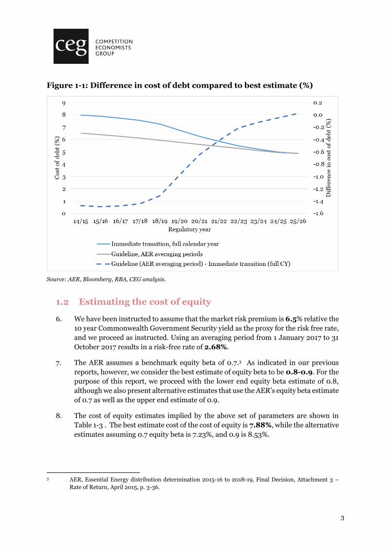
5. The cost of debt series under the base and alternative assumptions are shown in Table
1-2, while the differences in cost of debt estimates compared to the base assumptions
are also shown on the right-hand axis of Figure 3-3. As seen in Figure 1-1, the
Guideline transition using the AER’s averaging periods in the first two years
converges with the immediate trailing average two years after the end of the
transition.2
Table 1-2: Alternative estimates of cost of debt (2013 CY to 2023 CY)
Regulatory year
14/15 15/16 16/17 17/18 18/19 19/20
Immediate trailing average
7.98 7.89 7.73 7.55 7.26 6.75
AER Guideline*
6.51 6.40 6.25 6.10 5.94 5.77
Regulatory year
20/21 21/22 22/23 23/24 24/25 Ave.
Immediate trailing average
6.25 5.85 5.48 5.23 4.99 6.63
AER Guideline*
5.61 5.44 5.27 5.11 4.94 5.76
Source: AER, Bloomberg, RBA, CEG analysis; * AER estimates up to the 2017/18 regulatory year obtained
from: AER, Essential Energy Distribution Determination, 2017-18 return on debt update – PTRM, July 2017.
2 The 5 bp difference between the two approaches in the 2024/25 regulatory year is attributed to
assumptions 4.ii to 4.iv. Assuming that no further curve switches or retrospective updates are made to the
Bloomberg and RBA series, the estimates from the two approaches will eventually achieve exact
convergence.
3
Figure 1-1: Difference in cost of debt compared to best estimate (%)
Source: AER, Bloomberg, RBA, CEG analysis.
1.2 Estimating the cost of equity
6. We have been instructed to assume that the market risk premium is 6.5% relative the
10 year Commonwealth Government Security yield as the proxy for the risk free rate,
and we proceed as instructed. Using an averaging period from 1 January 2017 to 31
October 2017 results in a risk-free rate of 2.68%.
7. The AER assumes a benchmark equity beta of 0.7.3 As indicated in our previous
reports, however, we consider the best estimate of equity beta to be 0.8-0.9. For the
purpose of this report, we proceed with the lower end equity beta estimate of 0.8,
although we also present alternative estimates that use the AER’s equity beta estimate
of 0.7 as well as the upper end estimate of 0.9.
8. The cost of equity estimates implied by the above set of parameters are shown in
Table 1-3 . The best estimate cost of the cost of equity is 7.88%, while the alternative
estimates assuming 0.7 equity beta is 7.23%, and 0.9 is 8.53%.
3 AER, Essential Energy distribution determination 2015-16 to 2018-19, Final Decision, Attachment 3 –
Rate of Return, April 2015, p. 3-36.

4
Table 1-3: Cost of equity estimates
Estimate Risk-free rate Equity beta MRP Cost of equity
Best estimate 2.68% 0.8 6.5% 7.88%
Alternative 1 (AER) 2.68% 0.7 6.5% 7.23%
Alternative 2 2.68% 0.9 6.5% 8.53%
Source: AER, RBA, CEG analysis
1.3 WACC estimates
9. We are further instructed to make the following assumptions regarding other WACC
parameters:
Gearing: 60%;
Tax rate: 30%;
Gamma: 0.4.
10. The resulting vanilla WACC estimates for all six possible scenarios (2 debt scenarios
and 3 equity scenarios) are shown in Table 1-4, with corresponding pre-tax WACC
scenarios in Table 1-5.

5
Table 1-4: Vanilla WACC estimates under different scenarios
Debt Equity 14/15 15/16 16/17 17/18 18/19 19/20 20/21 21/22 22/23 23/24 24/25 Ave.
TA Beta 0.8
7.94 7.88 7.79 7.68 7.50 7.20 6.90 6.66 6.44 6.29 6.14 7.13
Guide (AER)
Beta 0.8
7.05 6.99 6.90 6.81 6.71 6.61 6.51 6.41 6.31 6.21 6.11 6.61
TA Beta 0.7
7.68 7.62 7.53 7.42 7.24 6.94 6.64 6.40 6.18 6.03 5.88 6.87
Guide (AER)
Beta 0.7
6.79 6.73 6.64 6.55 6.45 6.35 6.25 6.15 6.05 5.95 5.85 6.35
TA Beta 0.9
8.20 8.14 8.05 7.94 7.76 7.46 7.16 6.92 6.70 6.55 6.40 7.39
Guide (AER)
Beta 0.9
7.31 7.25 7.16 7.07 6.97 6.87 6.77 6.67 6.57 6.47 6.37 6.87
Source: AER, Bloomberg, RBA, CEG analysis.

6
Table 1-5: Pre-tax WACC estimates under different scenarios
Debt Equity 14/15 15/16 16/17 17/18 18/19 19/20 20/21 21/22 22/23 23/24 24/25 Ave.
TA Beta 0.8
8.63 8.58 8.48 8.37 8.19 7.89 7.59 7.35 7.13 6.98 6.83 7.82
Guide (AER)
Beta 0.8
7.75 7.68 7.59 7.51 7.41 7.31 7.21 7.11 7.01 6.91 6.81 7.30
TA Beta 0.7
8.31 8.26 8.16 8.05 7.88 7.57 7.28 7.04 6.81 6.66 6.52 7.50
Guide (AER)
Beta 0.7
7.43 7.36 7.28 7.19 7.09 6.99 6.89 6.79 6.69 6.59 6.49 6.98
TA Beta 0.9
8.95 8.89 8.80 8.69 8.51 8.21 7.91 7.67 7.45 7.29 7.15 8.14
Guide (AER)
Beta 0.9
8.06 8.00 7.91 7.82 7.72 7.62 7.52 7.42 7.32 7.22 7.12 7.61
Source: AER, Bloomberg, RBA, CEG analysis

7
2 Introduction
11. My name is Tom Hird. I have a Ph.D. in Economics and 20 years’ experience as a
professional economist. My curriculum vitae is provided separately. This report has
been prepared to provide Essential Energy with an estimate of the appropriate cost
of debt that should apply to it for the 2019-24 regulatory cycle.
12. I acknowledge that I have read, understood and complied with the Federal Court of
Australia’s Practice Note CM 7, Expert Witnesses in Proceedings in the Federal Court
of Australia.
13. I have been assisted in the preparation of this report by Johnathan Wongsosaputro,
Ker Zhang, and Yang Hao from CEG’s Sydney office. However, the opinions set out
in this report are my own.
Thomas Nicholas Hird
8 November 2017
2.1 Report structure
14. The remainder of this report has the following structure:
Section 3 sets out our estimates of Essential Energy’s cost of debt, as well as the
assumptions and underlying reasoning behind our estimates;
Section 4 sets out our estimates of Essential Energy’s cost of equity; and
Section 5 calculates the set of WACC estimates under various alternative
scenarios for the cost of debt and equity.

8
3 Best estimate of cost of debt
15. In this section we set out and justify the underlying assumptions that we have made
in arriving at our recommendation for the best estimate of the cost of debt that should
apply to Essential Energy over the 2019-24 regulatory cycle. Where appropriate, we
also make references to the regulatory precedence available for each component of
the cost of debt.
3.1 Best estimate of cost of debt
16. We have made the following assumptions when generating our estimates:
10-year benchmark debt term;
Immediate trailing average approach for the cost of debt transition;
Spread to swap estimates sourced from the simple average of RBA and
Bloomberg 10-year yield estimates over the entire period;
Bloomberg series switches from BFV to BVAL after 30 April 2014;
Full calendar year as the averaging period for each regulatory year;4
Use RBA and Bloomberg data that has been retrospectively updated; and
BBB curves being used to generate spread to swap estimates.
17. Under the above set of assumptions and using a 10-year trailing average, the best
estimates for cost of debt over the 11 years starting from the first year of the transition
to the first year after the transition (2013 CY to 2023 CY) are shown in Table 3-1. As
requested by Essential Energy, the estimates for 2018 and all future years have been
generated under the assumption that future base rates and spreads are assumed to
be equal to the 2017 placeholder values, and are thus equal to the corresponding
estimates obtained from the months of January 2017 to October 2017.
Table 3-1: Best estimates of cost of debt (2013 CY to 2023 CY)
2013 2014 2015 2016 2017 2018
7.98 7.89 7.73 7.55 7.26 6.75
2019 2020 2021 2022 2023 Average
6.25 5.85 5.48 5.23 4.99 6.63
Source: AER, Bloomberg, RBA, CEG analysis
4 We use 1 January 2017 to 31 October 2017 as the placeholder averaging period in place of the 2017 calendar
year.

9
3.2 Debt term
18. Australian electricity distributors have historically been assigned a benchmark debt
term of 10 years. This estimate has considerable support in terms of regulatory
precedence and empirical evidence.5
19. The same debt term is also being applied to Essential Energy in its current regulatory
cycle:6
Consistent with the Guideline and draft decision, we are satisfied that a
return on debt estimated based on a 10 year benchmark debt term, BBB+
benchmark credit rating, and using an independent third party data series
is commensurate with the efficient financing costs of a benchmark efficient
entity.
20. We therefore proceed in accordance with our instructions that the benchmark debt
term is assumed to be 10 years.
3.3 Debt management strategy
21. There have so far been four main proposed methods for approaching the transition
from the AER’s previous on-the-day approach for calculating the regulatory
allowance on debt towards a trailing average approach.
22. These four approaches are:
i. Immediate trailing average (0% swaps);
ii. Hybrid (100% swaps);7
iii. Optimal hedging (33% swaps); and
iv. AER guideline transition.
5 See, for example: CEG, Debt strategies of utility businesses, June 2013; CEG, Debt staggering of Australian
businesses, December 2014.
6 AER, Essential Energy distribution determination 2015-16 to 2018-19, Final Decision, Attachment 3 –
Rate of return, April 2015, p. 3-192.
7 One Victorian energy business previously proposed the hybrid approach in which the transition was
applied only to the base rate, while spreads were calculated on an immediate trailing average basis.
However, this approach was only proposed as a third preference and has not gained further traction since.
I therefore do not consider this approach further in this report.
See: AGN, Response to Draft Decision: Rate of Return, Attachment 10.26, January 2016, p. 7; cited in:
AER, Australian Gas Networks Access Arrangement 2016 to 2021, Final Decision, Attachment 3 – Rate of
Return, May 2016, p. 3-311.

10
23. As indicated by the parentheses above, approaches 22.i to 22.iii each correspond to
the cost of debt that would have been incurred as a result of applying a particular debt
management strategy.
24. Specifically, these three approaches reflect the cost of debt for firms that utilise
different levels of hedging on their debt obligations, with the immediate trailing
average corresponding to a firm that left all its debt unhedged, the hybrid to a firm
that hedged the entirety of the base rate component of its debt to a five-year term,
and the optimal hedge to a firm that only hedged 1/3 of its debt.8 The AER guideline
transition approach does not correspond to a particular debt management strategy
and cannot be fully replicated in practice by a DNSP that seeks to match its debt
allowance with its actual debt costs.
25. We discuss the above debt management approaches in sections 3.3.1 to 3.3.2. As
instructed, we proceed on the assumption that the immediate trailing average
approach is used.
3.3.1 Essential Energy uses a staggered debt profile that is left unhedged
26. Essential Energy, while it was still part of Networks NSW, maintained a staggered
debt profile that is left unhedged. That is, Essential Energy did not utilise interest rate
swaps in order to reduce the term of its debt from 10 years down to a shorter 5-year
term:9
One of the key bases for Essential Energy's and the other NSW service
providers' proposals in favour of a backwards looking trailing average
relates to their actual financing practices. While Essential Energy managed
its refinancing risk, it did not take steps to actively manage its interest rate
risk.
27. It is important to note that, in its later decisions for the Victorian energy businesses,
the AER expressed the view that both the on-the-day and trailing average approaches
allow service providers the reasonable opportunity to recover at least efficient costs
8 See: CEG, Efficient use of interest rate swaps to manage interest rate risk, June 2015.
9 AER, Essential Energy distribution determination 2015-16 to 2018-19, Final Decision, Attachment 3 –
Rate of Return, April 2015, p 3-153.

11
over the term of the RAB, although the AER couched the latter as requiring a full
transition when switching between regimes:10, 11
That is, mathematically, we demonstrate that in principle:
• The on-the-day approach service providers [sic] with the reasonable
opportunity to recover at least efficient costs over each regulatory period
and over the term of the RAB.
• The trailing average approach provides service providers with the
reasonable opportunity to recover at least efficient costs over the term of
the RAB.
If switching between regimes, a full transition provides service providers
with a reasonable opportunity to recover at least efficient costs over the
term of the RAB. That is, the same ex-ante compensation should be achieved
under: an on-the-day regime, a trailing average regime, or a switch from
one regime to the other (but only if the switch is revenue neutral).
28. We note as well that maintaining an unhedged staggered debt profile is also
consistent with the commercial practices of Australian unregulated firms.12
3.3.2 Regulatory developments concerning cost of debt transition
29. Given that the Networks NSW businesses each maintained a staggered debt profile
that was left unhedged, the businesses submitted that there was no need for a
transition towards a trailing average to be applied to them, and that an immediate
adoption of the trailing average would instead be appropriate:13
The NSW DNSPs have managed their debt using a staggered portfolio
approach and as a result would not face any difficulty transitioning to the
trailing average approach. The NSW DNSPs propose an immediate
transition to the trailing average approach.
10 AER, AusNet Services transmission determination 2017-2022, Final Decision, Attachment 3 – Rate of
Return, April 2017, p. 3-299.
11 I note that I have considerable concerns regarding the assumptions that the AER used for arriving at its
conclusions for the on-the-day approach, but the on-the-day approach is not used in this report and will
therefore not be discussed further.
12 CEG, Debt staggering of Australian businesses, December 2014.
13 NNSW, Ausgrid Endeavour and Essential cost of debt averaging periods, Letter from Vince Graham (CEO
of NNSW) to AER, February 2014, p. 3.

12
30. The AER was not persuaded by the above argument and decided to enforce the full
transition from the on-the-day approach to the trailing average approach.14 Networks
NSW lodged an appeal to the Australian Competition Tribunal regarding this issue
(and other issues), for which the subsequent decision was further appealed by the
AER to the Full Court of the Federal Court of Australia.15
31. The Full Court appears to have held that the Tribunal had found that Networks NSW’s
existing unhedged staggered debt profile did not require a transition to be applied:16
548 …The point of present significance is that the Tribunal concluded that
no transition was required for the NSW service providers (because they
already had in place a financing cost structure that was amenable to the
new (trailing average) methodology) and that r 6.5.2(k)(4) did not require
otherwise.
32. The Full Court’s analysis also appears to agree with the Tribunal’s conclusion based
on substantially similar grounds – that since Networks NSW had already adopted a
debt management strategy that was amenable to the trailing average, then there were
no impacts that needed to be unwound by implementing a transition in the way that
the AER had done [emphasis added]:17
572 At the commencement of the new regulatory period, the NSW service
providers already had in place a debt structure that was both their
particular response to the previous on-the-day approach to estimating the
return on debt and, as it happened, a debt structure that was amenable to
the “changed” methodology of the trailing average approach which the AER
had decided to adopt. Significantly, in each case, that debt structure was
not one complicated by the overlay of hedging contracts that needed to be
unwound. The consequence of this was that, when the AER came to consider
r 6.5.2(k)(4) in relation to those service providers, there were no impacts
(in the form of hedging contracts that needed to be unwound) apposite to
the benchmark efficient entity (or each benchmark efficient entity) for each
such service provider that could be said to have arisen from the AER’s
change in methodology from the on-the-day approach to the trailing
average approach. Given that there were no such impacts, there
was no need for the AER to take a step which, in the
circumstances, r 6.5.2(k)(4) did not require for those service
providers, namely a transition to the trailing average approach
14 AER, Essential Energy distribution determination 2015-16 to 2018-19, Final Decision, Attachment 3 –
Rate of Return, April 2015, p 3-155.
15 Australian Energy Regulator v Australian Competition Tribunal (No 2) [2017] FCAFC 79.
16 Australian Energy Regulator v Australian Competition Tribunal (No 2) [2017] FCAFC 79 at [548].
17 Australian Energy Regulator v Australian Competition Tribunal (No 2) [2017] FCAFC 79 at [572]-[573].

13
of estimating the return on debt by adopting a mechanism to
unwind hedging contracts, such as that reflected in Option 2.
573 The same conclusion applies with respect to ActewAGL. Even though
it held no debt, it was nonetheless necessary for the AER to arrive at an
estimate for its return on debt in accordance with the allowed rate of return
objective in r 6.5.2(c) so as to achieve the purposes of the return on capital
building block. Even so, there was no meaningful, relevant impact
on the benchmark efficient entity apposite for ActewAGL that
could be said to have arisen from the change in methodology for
estimating its allowed rate of return. The occasion or need for a
transition simply did not exist.
33. In response to the AER’s assertion that Networks NSW’s debt structure was ‘not
efficient in light of the “on-the-day” approach’ and that ‘an efficient entity would have
managed interest rate risk’,18 the Full Court reaffirmed its conclusion that the
Tribunal was not in error on this issue and that no transition was required for the
NSW service providers [emphasis added]:19
593 Thirdly, with respect to the AER’s submissions recorded at [580]
above, we repeat our conclusion that the Tribunal did not err in its
construction and application of r 6.5.2(k)(4). No transitioning was
required in the case of the electricity network respondents by
reason of the change in methodology from the on-the-day
approach to the trailing average approach to estimate the return
on debt. So far as the NSW service providers were concerned, the Tribunal
left open the question of whether their portfolios of staggered fixed rate debt
were efficient in form. No judicially reviewable error is made out in the
Tribunal’s conclusion that, if not, the efficient financing costs of the
benchmark efficient entity would apply prospectively.
34. Consistent with the Full Court’s views, our analysis in this report also proceeds on the
assumption that an immediate trailing average is to be applied when calculating
Essential Energy’s debt allowance.
3.4 Base rate
35. The AER uses interest rate swaps as the proxy for the base rate component of the cost
of debt in its extrapolation methodology, as opposed to other candidates such as
Commonwealth Government Securities.
18 Australian Energy Regulator v Australian Competition Tribunal (No 2) [2017] FCAFC 79 at [572]-[580].
19 Australian Energy Regulator v Australian Competition Tribunal (No 2) [2017] FCAFC 79 at [593].

14
36. The AER explained that this choice was made in accordance with market
convention:20
Traditionally, we have measured the DRP relative to the 10 year CGS rate.
This was for consistency with how we measure the risk free rate component
of the return on equity. However, market convention is to measure the DRP
relative to the swap rate. As Chairmont stated:
The DRP used throughout this document is the interest rate premium for
the corporate borrower over the swap rate, because practical financial
management requires companies to use swaps. The AER measurement
of DRP is the premium above the CGS rate(s); however CGS(s) are not a
relevant instrument for corporates.
In this decision, we refer to the swap rate when we refer to the 'base rate
component' of the return on debt. And we mostly refer to the DRP over the
swap rate when we refer to the DRP.
37. In this report, I proceed with the same assumption that the 10-year rate on interest
rate swaps is to be used as the base rate of the cost of debt.
3.5 Spread
38. As explained in section 3.4, the AER measures the base rate component of the cost of
debt using the 10-year swap rate. In turn, the spread to swap is used as the measure
of the risk premium. Unlike the base rate, which is consistent across all firms, the
spread to swap varies across firms and is affected primarily by the credit rating of the
firm of interest.
3.5.1 Credit rating
39. Australian DNSPs have historically been assigned a BBB+ benchmark credit rating –
a decision that is supported by empirical analysis.
40. CEG previously carried out an empirical analysis of the AER’s sample of regulated
utilities, and found that the median credit rating for the sample was BBB+ on average
over the period 2002 to 2012. However, the analysis also showed that there appeared
to have been a sustained drop in median credit ratings for the sample from A- in 2002
to BBB since 2009.21 This can be seen in Table 3-2, which reproduces Table 1 of the
previous CEG memorandum.
20 AER, Essential Energy distribution determination 2015-16 to 2018-19, Final Decision, Attachment 3 –
Rate of Return, April 2015, pp. 3-161.
21 CEG, Factors relevant to estimating a trailing average cost of debt, Memorandum, May 2014.

15
Table 3-2: Median credit rating for AER sample by year (reproduces Table 1 of CEG’s 2014 memorandum)
2002 2003 2004 2005 2006 2007 2008 2009 2010 2011 2012 2013
A- BBB+ BBB+ BBB+ BBB+ BBB+ A- BBB BBB BBB BBB BBB
Source: Bloomberg, CEG analysis
41. The AER has also updated its credit rating analysis up to the year 2016 as part of its
final decisions for the Victorian energy businesses.22 Table 3-3 provides a further
update for 2017, with the 2017 data being collected as at 26 September 2017. It can
be seen that the median credit rating of the AER’s preferred sample of comparators
remains at BBB+.
22 AER, AusNet Services transmission determination 2017-2022, Final Decision, Attachment 3 – Rate of
Return, April 2017, p. 3-351.

16
Table 3-3: Credit ratings of network service providers over time
Issuer 2006 2007 2008 2009 2010 2011 2012 2013 2014 2015 2016 2017
APT Pipelines Ltd
NR NR NR BBB BBB BBB BBB BBB BBB BBB BBB BBB
ATCO Gas Australian LP
NR NR NR NR NR BBB BBB A- A- A- A- BBB+
DBNGP Trust BBB BBB BBB BBB- BBB- BBB- BBB- BBB- BBB- BBB- BBB- BBB
DUET Group BBB- BBB- BBB- BBB- BBB- BBB- BBB- NR NR NR NR NR
ElectraNet Pty Ltd
BBB+ BBB+ BBB+ BBB BBB BBB BBB BBB BBB+ BBB+ BBB+ BBB+
Energy Partnership (Gas) Pty Ltd
BBB BBB BBB- BBB- BBB- BBB- BBB- BBB- BBB- BBB- BBB- BBB
Australian Gas Networks Ltd
BBB- BBB- BBB- BBB- BBB- BBB- BBB- BBB BBB+ BBB+ BBB+ BBB+
ETSA Utilities A- A- A- A- A- A- A- A- A- A- A- A-
Powercor Australia LLC
A- A- A- A- A- A- A- BBB+ BBB+ NR NR NR
AusNet Services
A A A- A- A- A- A- A- A- A- A- A-
SGSP Australia Assets Pty Ltd
NR NR A- A- A- A- A- BBB+ BBB+ BBB+ A- A-
The CitiPower Trust
A- A- A- A- A- A- A- BBB+ BBB+ NR NR NR
United Energy Distribution Pty Ltd
BBB BBB BBB BBB BBB BBB BBB BBB BBB BBB BBB BBB+
Victoria Power Networks Pty Ltd
NR NR NR NR NR NR NR NR NR BBB+ BBB+ BBB+
Median (year) BBB/BBB+
BBB/BBB+
BBB+ BBB BBB BBB BBB/BBB+
BBB+ BBB+ BBB+ BBB+ BBB+
Source: Bloomberg, Standard and Poor’s, AER analysis, CEG analysis
3.5.2 Data sources
42. Third party sources generally do not publish a BBB+ credit rating curve for Australian
bonds, possibly because of the sparse availability of such bonds.
43. Instead, sources such as Bloomberg, RBA, and Reuters only publish “broad” rating
curves, such as “broad BBB” curves that are fitted on a sample containing bonds with
ratings ranging from BBB- to BBB+, and “broad A” curves that are fitted on bonds
with ratings ranging from A- to A+.
17
44. The AER’s convention when dealing with this issue is to use the 10-year estimate
obtained from one or more of the “broad BBB” curves. We proceed with the same
convention.
3.5.2.1 RBA: Extrapolation using AER methodology
45. The RBA curve is published for the 3-year, 5-year, 7-year, and 10-year target tenors.
Due to empirical asymmetries in the time to maturity of the RBA’s sample of bonds,
however, the effective tenors of the estimates tend to be below their respective targets.
The established regulatory practice in Australia for ameliorating this issue is to use
extrapolation to extend the effective tenors of the estimates to 10 years.
46. The AER’s preferred methodology is to linearly extrapolate the RBA curve based on
the spread between the estimates for the 7-year and 10-year target tenors. The exact
details of this method have been set out in the 2015 Final Decision for Essential
Energy.23 We adopt this approach for the purpose of this report.
3.5.2.2 RBA: Retrospective updating of data
47. From the time when the RBA began publishing its series of Australian corporate bond
spreads and yields, the series has been retrospectively updated twice. This occurred
in August 2015 and in May 2017. In each case, the RBA retrospectively adjusted its
estimates in prior years.
48. The RBA explained that the 2015 adjustment was implemented in order to “reflect
improvements to methodology and data”, although no further explanation was
provided for the 2017 adjustment.24
49. For the purpose of this report, we proceed on the assumption that the latest RBA
series is used, with retrospective adjustments being incorporated into the estimates.
50. We note, however, that the AER’s preference is to refrain from making retrospective
updates to the Bloomberg or RBA curves [emphasis added]:25
[Event]
23 AER, Essential Energy distribution determination 2015-16 to 2018-19, Final Decision, Attachment 3 –
Rate of Return, April 2015, pp. 3-549 to 3-552.
24 RBA, Changes to Statistical Tables, accessed on 23 October 2017. Available at:
http://www.rba.gov.au/statistics/tables/changes-to-tables.html
25 AER, AusNet Services transmission determination 2017-2022, Final Decision, Attachment 3 – Rate of
Return, April 2017, p. 3-362.

18
Either Bloomberg or RBA substitutes its current methodology for a revised
or updated methodology.
[Changes to approach]
We will adopt the revised or updated methodology. Then, at the next
regulatory determination, we will review this updated methodology. As
noted above, we would also review any new data sources.
However, if Bloomberg or the RBA backcasts or replaces data
using a revised or updated methodology we will not use the
backcasted data to re-estimate our estimates of the prevailing
return on debt for previous years. This would be impractical and
would create regulatory uncertainty over whether the allowed return on
debt would at some point in the future be re-opened. Instead, we will
continue to use the Bloomberg or RBA data that we downloaded
at the time of estimating the prevailing return on debt for that
point in time.
51. However, this policy may be interpreted as only applying once the AER has already
used the data in a price setting context. The AER has not done so for Essential Energy
yet so this rationale for not using backcasted data does not apply.
3.5.2.3 Bloomberg: Switch from BFV to BVAL from 1 May 2014 onwards
52. Bloomberg currently publishes two AUD broad-BBB curves for Australian corporate
bonds – the older Bloomberg Fair Value (BFV) curve and the more recent Bloomberg
Valuation Service (BVAL) curve. Australian regulators currently favour the use of the
BVAL curve for various reasons, such as the availability of a 10-year estimate.26
53. However, the methodology for neither publication is transparent so it is not possible
to provide a meaningful discussion of any differences in methodology that might
cause the BVAL estimates to be more reliable than the BFV estimates.
54. One important issue for deriving Bloomberg estimates of the spread to swap is the
exact date of the transition from the BFV curve to the BVAL curve, since the latter is
only available from 22 June 2009 and was initially published up to a 3-year tenor.
CEG has previously carried out an assessment of the BVAL curve and found that,
prior to May 2014, the curve did not behave in a manner that was consistent with
reasonable expectations.27
26 The longest tenor of the AUD BBB BFV curve is currently 7 years.
27 CEG, Criteria for assessing fair value curves, January 2016.

19
55. The Bloomberg BVAL curve was only introduced in 2013 and has since been extended
backwards in time by Bloomberg to mid-2010. As such, it does not extend sufficiently
to include the 2008/09 crisis. The BVAL curve is the most erratic of the three curves
(BVAL, RBA and the discontinued CBA Spectrum curves) published over the same
time period – with large single day changes in estimated yields. For example, from 1
August 2011 to 3 August 2011 the extrapolated28 BVAL spread rose from 2.47% to
3.18% (as can be seen in Figure 3-1).
Figure 3-1: Reproduction of Figure 9 from May 2014 report - RBA, CBASpectrum and Bloomberg29
Source: RBA, Bloomberg, CBASpectrum and CEG analysis
56. The BVAL information from before 1 May 2014 is also intermittent, as is illustrated
in Figure 3-2. In addition, prior to that date the BVAL curve provides results that are
28 We have extrapolated the BVAL curve from 7 to 10 years in the same manner as the BFV curve.
29 The Bloomberg BBB fair value estimate shown in the chart is, where necessary, extrapolated to 10 years
consistent with regulatory precedent as follows: until 22 June 2010, the BBB curve is extrapolated to 10
years based on the slope of the fair value curve closest to BBB in rating (ie, A, AA and AAA in order of
preference); between 23 June 2010 and 31 October 2013, the BBB curve is extrapolated from 7 years to 10
years assuming an increase in DRP calculated as the average increase in DRP between 7 and 10 years for
the Bloomberg AAA fair value curve over the 20 days to 22 June 2010; and since 1 November 2013, the
BBB curve is extrapolated from 7 years to 10 years assuming no increase in DRP.

20
inconsistent with standard finance theory and the empirical regularity that the risk
premium on bonds tend to increase with the maturity of the bonds – especially
between one and seven years. However, the BVAL one year spread to swap is
substantially higher than the 7 year spread to swap from late 2012 until late 2013. In
fact, the one and two year curves are only below curves of longer maturities from the
beginning of May 2014, which is the time at which Bloomberg first introduced the
BVAL curve.
Figure 3-2: BVAL curves at different maturities
Source: Bloomberg, CEG analysis
57. Figure 3-2 clearly indicates that, prior to May 2014, the BVAL curve was not behaving
in a manner that is consistent with reasonable expectations. Beyond 2014 the
problem with the term structure appears to have been rectified.
58. The AER has so far not committed to a position regarding the precise date for
switching from the BFV curve to the BVAL curve, presumably because its preferred
guideline transition approach did not require one. Nonetheless, Chairmont
(consultant for the AER) has indicated a preference for 1 April 2010 as the starting
date for using the BVAL curve,30 but provided no justification for its assessment.
30 Chairmont, Cost of Debt: Transitional Analysis, April 2015, p. 41.

21
59. On the above basis we consider that Bloomberg estimates should be obtained from
the BFV curve until 30 April 2014, after which (from 1 May 2014 onwards) the
estimates are obtained from the BVAL curve (noting that in the post April 2014 period
the BFV and BVAL curves are almost identical in value for a published tenor).
3.5.2.4 Bloomberg: Extrapolation using AER methodology
60. The BFV curve is only published up to 7 years, while there are sporadic periods during
which the BVAL curve is published to tenors less than 10 years.31
61. The AER’s preferred methodology for obtaining 10-year estimates in such
circumstances is to linearly extrapolate the relevant curve based on the spread
between the estimates for the 7-year and 10-year target tenors of the RBA curve. The
exact details of this method have been set out in the 2015 Final Decision for Essential
Energy.32 We have adopted this approach for the purpose of this report.
3.5.2.5 Reuters: Possible candidate
62. The Reuters curve has recently arisen as a possible candidate for spread to swap
estimates. In its decisions for the Victorian energy businesses, the AER recently
considered the merits of the Reuters curve but did not form a definitive view of it,
instead indicating that the curve could be further considered in the future:33
For the reasons in this section and in Appendix A, and given AusNet Services
has not proposed we used Thomson Reuters curve, we remain satisfied that
a simple average of the BVAL and RBA curves will contribute to an estimate
that will achieve the ARORO. However, we have not yet formed a definitive
view on the suitability of the Reuters curve, and are open to further
considering this curve in the future.
63. We do not use Reuters in this report.
3.5.2.6 Weighting of sources
64. The AER’s preferred approach is to weight the RBA and Bloomberg curves equally by
taking a simple average of their spread to swap estimates. We have been instructed
to also proceed with a simple average of the RBA and Bloomberg curves. However,
31 For example, the BVAL curve is only published up to 5 years from 1 September 2016 to 6 September 2016,
and up to 4 years from 14 September 2016 to 4 October 2016.
32 AER, Essential Energy distribution determination 2015-16 to 2018-19, Final Decision, Attachment 3 –
Rate of Return, April 2015, pp. 3-549 to 3-551.
33 AER, AusNet Services transmission determination 2017-2022, Final Decision, Attachment 3 – Rate of
Return, April 2017, pp. 3-341 to 3-342.

22
we note that other averaging methods could also be employed.34 In addition, to the
extent that uneven weights were to be applied then we consider that more weight
should be given to the RBA curve because it is based on a materially larger sample of
bonds.
3.5.3 Averaging periods in 2013 and 2014
65. When making its decision for Networks NSW’s 2014-15 to 2018-19 regulatory cycle,
the AER required the businesses to nominate forward-looking averaging periods.
66. Due to the timing of the decision, the Networks NSW businesses were not able to
nominate the full 2013 and 2014 calendar years as their averaging periods, since both
of these had periods that were passed. The Networks NSW businesses thus
nominated the averaging period with the maximum number of observations (28
February 2014 to 30 June 2014 for the 2014-15 update and 1 July 2014 to 31
December 2014 for the 2015-16 update), but noted that this would still not be
consistent with a trailing average debt management strategy.35
67. As indicated in section 3.3, we proceed as instructed under the assumption that the
trailing average approach is the benchmark debt management strategy. Our analysis
therefore assumes that the averaging periods in each year are consistent with a
trailing average strategy, such that the full calendar year is always used as the
averaging period, including for the 2014-15 and 2015-16 updates.
3.6 Alternative cost of debt estimates
68. Essential Energy has further requested a cost of debt estimate based on the AER’s
Guideline approach, which uses the following assumptions:
i. AER Guideline full transition;
ii. Modified averaging periods for the 2014-15 and 2015-16 updates (28 February
2014 to 30 June 2014 and 1 July 2014 to 31 December 2014) followed by full
calendar years as the averaging period for each subsequent regulatory year;
iii. Bloomberg series switches from BFV to BVAL on 1 April 2010; and
iv. No retrospective updating of RBA data.
34 For example, some average of the Bloomberg, RBA, and Reuters curves could be used, or curve testing
could be used to choose the most appropriate curve, which would then be assigned 100% weight.
See: CEG, Curve testing and selecting averaging periods: A report for AGN, January 2016.
35 NNSW, Ausgrid Endeavour and Essential cost of debt averaging periods, Letter from Vince Graham (CEO
of NNSW) to AER, February 2014, p. 3.

23
69. The cost of debt series under the base and alternative assumptions are shown in Table
3-4, while the differences in cost of debt estimates compared to the base assumptions
are also shown on the right-hand axis of Figure 3-3. As seen in Figure 3-3, the
Guideline transition using the AER’s averaging periods in the first two years
converges with the immediate trailing average two years after the end of the
transition.36
Table 3-4: Alternative estimates of cost of debt (2013 CY to 2023 CY)
Regulatory year
14/15 15/16 16/17 17/18 18/19 19/20
Immediate trailing average
7.98 7.89 7.73 7.55 7.26 6.75
AER Guideline*
6.51 6.40 6.25 6.10 5.94 5.77
Regulatory year
20/21 21/22 22/23 23/24 24/25 Ave.
Immediate trailing average
6.25 5.85 5.48 5.23 4.99 6.63
AER Guideline*
5.61 5.44 5.27 5.11 4.94 5.76
Source: AER, Bloomberg, RBA, CEG analysis; * AER estimates up to the 2017/18 regulatory year obtained
from: AER, Essential Energy Distribution Determination, 2017-18 return on debt update – PTRM, July 2017.
36 The 5 bp difference between the two approaches in the 2024/25 regulatory year is attributed to
assumptions 68.ii to 68.iv. Assuming that no further curve switches or retrospective updates are made to
the Bloomberg and RBA series, the estimates from the two approaches will eventually achieve exact
convergence.

24
Figure 3-3: Difference in cost of debt compared to best estimate (%)
Source: AER, Bloomberg, RBA, CEG analysis.

25
4 Best estimate of cost of equity
70. In this section we set out and justify the underlying assumptions that we have made
in arriving at our best estimate of the cost of equity that should apply to Essential
Energy over the 2019-24 regulatory cycle.
71. We have been instructed to assume that the market risk premium is 6.5% relative to
the prevailing 10 year Commonwealth Government Securities (CGS) rate, and we
proceed as instructed.
4.1 Risk-free rate
72. The AER estimates the risk-free rate based on the 10-year yield of Commonwealth
Government Securities (CGS):37
The risk free rate is determined by observing the return on ten-year
Commonwealth Government Securities over a short period close to the start
of the next regulatory period.
73. In this report, we use the same methodology to derive the risk-free rate that applies
to the cost of equity, based on an averaging period from 1 January 2017 to 31 October
2017. This results in a risk-free rate of 2.68%.
4.2 Equity beta
74. The AER assumes a benchmark equity beta of 0.7, which is selected as the upper
bound of its equity beta range (0.4 to 0.7).38 However, we consider the best estimate
of equity beta to be between 0.8-0.9. For the purpose of this report, we proceed with
the lower end equity beta estimate of 0.8, although we also present alternative
estimates that use the AER’s equity beta estimate of 0.7, as well as the upper end
estimate of 0.9.
75. Our best estimate of 0.8-0.9 equity beta is drawn from recent empirical evidence,
which shows that there has been a recent sustained increase in equity beta reflecting
a structural break in equity beta estimates. In addition, it is well-documented in
literature that the Sharpe-Lintner CAPM, which the AER relies on for equity beta
estimates, tends to suffer from a “low beta bias”. These two factors suggest that the
37 AER, Better regulation: Rate of return guideline, December 2013, p. 2.
38 AER, Essential Energy distribution determination 2015-16 to 2018-19, Final Decision, Attachment 3 –
Rate of Return, April 2015, p. 3-36.

26
AER’s equity beta value of 0.7 is likely to be too low, such that an estimate between
0.8 and 0.9 would be a better estimate.
4.2.1 Estimates of beta
76. The empirical estimates of equity beta for the Australian sample of comparators has
increased recently, and continues to increase.
77. We have addressed the best estimate of equity beta most recently in a report for
AusNet using data to October 2016.39 Updating our estimates for the extra year of
data strengthens our conclusions in that report. Table 4-1 shows a comparison
between the estimated re-levered equity beta since October 2016 till October 2017
based on the methodology adopted by Henry (2014).40 The analysis is based on the
weekly return data, net debt and market capitalisation of each firm.
78. The result shows that the re-levered equity betas for the longest sample period for all
four comparators have either remained the same or increased by a small margin since
October 2016. The 5 year re-levered equity betas have increased for 3 of the 4
comparators and the increases range from 0.13 to 0.22. As a result, the average 5 year
re-levered equity beta has increased from 0.68 to 0.81. The 3 year re-levered equity
beta has also increased for 3 of the 4 comparator firms.
Table 4-1: Individual re-levered equity beta since October 2016 (re-levered to 60% gearing)
3 year 5 year Longest Period
Ending October 2016
Ending October 2017
Ending October 2016
Ending October 2017
Ending October 2016
Ending October 2017
APA 1.01 1.05 0.81 0.97 0.71 0.72
DUE41 0.38 0.51 0.28 0.41 0.35 0.37
SKI 1.17 1.14 0.83 1.05 0.66 0.68
AST 0.81 0.80 0.81 0.80 0.39 0.40
Source: CEG analysis using Bloomberg data
79. During the period, Duet Group was purchased by Cheung Kong Group. As a result its
equity ceased trading in mid-2017. If the 5 year re-levered equity beta is calculated
based on the remaining 3 Australian comparators, it would raise the 5 year equity
39 CEG, Replication and extension of Henry’s beta analysis, November 2016.
40 Olan T. Henry, Estimating 𝛽: An update, April 2014
41 Calculated to 16/1/2017, when the DUET Group board announced that it has agreed to the takeover bid
by Cheung Kong Group.

27
beta to 0.94. The longest series re-levered equity beta would also increase from 0.53
to 0.60.
80. The trend in 5 year re-levered equity beta is shown in Figure 4-1. It shows that the re-
levered equity beta began increasing since late 2013 to early 2014. The rate of increase
for the remaining 3 Australian comparators is much larger compared to Duet Group.
We have previously identified a structural break in the trend of equity beta which
indicated that the longest series estimate of equity beta is a biased estimate of betas
most likely to be observed in the near term future.42 Since that report was published,
the trend in 5 year re-levered equity beta has been sustained – consistent with finding
that a structural break occurred. This further indicates that the estimation of equity
likely to be observe in the near term future should focus on more recent periods rather
than the longest series.
Figure 4-1: Rolling 5 year re-levered equity beta
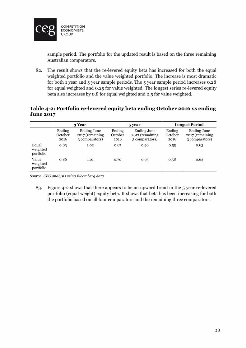
81. Table 4-2 shows the updated portfolio re-levered equity beta since October 2016.
Following the methodology adopted by Henry (2014), the portfolio in the November
2016 report is constructed using the 4 comparators based on equal weight and
weighted by market capitalisation. The weight by market capitalisation is calculated
based on the average market capitalisation of each of the four firms over the relevant
42 CEG, Estimating beta to be used in the Sharpe-Lintner CAPM, February 2016, Section 5
28
sample period. The portfolio for the updated result is based on the three remaining
Australian comparators.
82. The result shows that the re-levered equity beta has increased for both the equal
weighted portfolio and the value weighted portfolio. The increase is most dramatic
for both 1 year and 5 year sample periods. The 5 year sample period increases 0.28
for equal weighted and 0.25 for value weighted. The longest series re-levered equity
beta also increases by 0.8 for equal weighted and 0.5 for value weighted.
Table 4-2: Portfolio re-levered equity beta ending October 2016 vs ending June 2017
3 Year 5 year Longest Period
Ending October
2016
Ending June 2017 (remaining 3 comparators)
Ending October
2016
Ending June 2017 (remaining 3 comparators)
Ending October
2016
Ending June 2017 (remaining 3 comparators)
Equal weighted portfolio
0.83 1.02 0.67 0.96 0.55 0.63
Value weighted portfolio
0.86 1.01 0.70 0.95 0.58 0.63
Source: CEG analysis using Bloomberg data
83. Figure 4-2 shows that there appears to be an upward trend in the 5 year re-levered
portfolio (equal weight) equity beta. It shows that beta has been increasing for both
the portfolio based on all four comparators and the remaining three comparators.

29
Figure 4-2: Rolling 5 year portfolio re-levered equity beta (equal weight)
84. In sum, the recent empirical evidence supports an increase in the benchmark equity
beta from the previous 0.7 estimate to a range of 0.8-0.9.
85. All of the more recent evidence confirms the conclusion of our February 2016 report43
that there has been a structural break in Australia utility beta estimates and that more
recent betas are more representative of betas likely to be observed in the near future
than the historical average betas.
4.2.2 Low beta bias
86. A key shortcoming of the Sharpe-Lintner CAPM (SL-CAPM), is that the SL-CAPM is
empirically known to suffer from a “low beta bias”. That is, the SL-CAPM tends to
underestimate the returns of companies with beta below 1.0 (and overestimate
returns for companies with beta above 1.0).
87. Even if one were to ignore the most recent evidence as set out in the previous section
and instead adopt a best estimate of equity beta of 0.55 (the middle of the AER range),
pairing this 0.55 estimate with a low 𝑍𝐵𝑃
𝑀𝑅𝑃 estimate of 0.61 would still result in an
equity beta of 0.8.
43 CEG, Estimating beta to be used in the Sharpe-Lintner CAPM, February 2016, Section 5

30
88. Sections 4.2.2.1 to 4.2.2.3 explain the theoretical framework that underpins the 𝑍𝐵𝑃
𝑀𝑅𝑃
parameter, and demonstrate that reasonable adjustments for low beta bias will still
produce equity beta estimates that are higher than the AER’s benchmark value of 0.7.
4.2.2.1 Black CAPM
89. The low beta bias observed with the SL-CAPM can be corrected in several ways, with
CEG’s preferred method being the Black CAPM model, which includes a zero-beta
premium (ZBP) that adjusts for low beta bias.
90. The Sharpe-Lintner CAPM assumes that investors can borrow at the risk free rate to
invest in risky equities. The theoretical insight of the Black CAPM is that, when this
assumption is relaxed, the required return on low beta stocks increases relative to the
predictions of the Sharpe Lintner CAPM. This can be mathematically represented as
follows:
𝑅𝑆𝐿 𝐶𝐴𝑃𝑀 = 𝑅𝐹𝑅 + 𝛽 × 𝑀𝑅𝑃 Eqn. 1
𝑅𝐵𝑙𝑎𝑐𝑘 𝐶𝐴𝑃𝑀 = 𝑅𝐹𝑅 + 𝑍𝐵𝑃 + 𝛽 × (𝑀𝑅𝑃 − 𝑍𝐵𝑃) Eqn. 2
91. Algebraically rearranging Eqn 1 and Eqn 2 results in the following empirical estimate
of bias:
𝐵𝑖𝑎𝑠 = 𝑅𝐵𝑙𝑎𝑐𝑘 𝐶𝐴𝑃𝑀 − 𝑅𝑆𝐿 𝐶𝐴𝑃𝑀 = 𝑍𝐵𝑃 × (1 − 𝛽) Eqn. 3
92. Regulators have acknowledged that low beta bias is a problem with the SL CAPM.
The AER has referred to this as a reason to select a value of beta from the top of their
range [emphasis added]:44
The theoretical principles underpinning the Black CAPM—for firms with an
equity beta below 1.0, the Black CAPM may predict a higher return on
44 AER, Essential Energy distribution determination 2015-16 to 2018-19, Attachment 3 – Rate of return,
Final Decision, April 2015, p. 3-431 to 3-432.
Also see: AER, Essential Energy distribution determination 2015-16 to 2018-19, Attachment 3 – Rate of
return, Final Decision, April 2015, p. 3-36 [emphasis added]:
In informing the equity beta point estimate (from within the empirical range), we consider
evidence from other relevant material. This includes international empirical estimates
(set out in section D.3 of appendix D–equity beta) and the theoretical
underpinnings of the Black CAPM. This other information does not specifically indicate
which equity beta estimate we should choose from within our range. However, for reasons
discussed in section D.5.2 of appendix D–equity beta, we consider a point estimate of 0.7 is
reasonably consistent with these sources of information and is a modest step down from our
previous regulatory determinations. Choosing a point estimate at the upper end of our
range also recognises the uncertainty inherent in estimating unobservable
parameters, such as the equity beta.
31
equity than the SLCAPM. We consider this information points to the
selection of an equity beta point estimate above the best empirical estimate
implied from Henry's 2014 report.
However, we do not consider the theory underlying the Black CAPM
warrants a specific uplift or adjustment to the equity beta point estimate.
The theory underlying the Black CAPM is qualitative in nature, and we are
satisfied that this information is reasonably consistent with an equity
beta point estimate towards the upper end of our range (see section
D.4).
93. Following the views set out above, the AER decided to adopt a benchmark equity beta
value of 0.70.
4.2.2.2 Framework for adjusting equity beta to account for low beta bias
94. Although the AER has not set out a mathematical derivation of its equity beta
adjustment, this can be fitted into the framework in section 4.2.2.1 as follows:
A𝑚𝑒𝑛𝑑𝑒𝑑 𝑅𝑆𝐿 𝐶𝐴𝑃𝑀 = 𝑅𝐹𝑅 + 𝛽∗ × 𝑀𝑅𝑃 Eqn. 4
𝛽∗ = 𝛽 +𝑍𝐵𝑃
𝑀𝑅𝑃∗ (1 − 𝛽) Eqn. 5
where β* is the adjusted equity beta that corrects for the low beta bias.
95. The value of 𝑍𝐵𝑃
𝑀𝑅𝑃 in equation 5 should be derived from studies that attempt to estimate
the actual relationship between the measured beta of a stock (or, more often, a
portfolio of stocks with similar beta) and the actual return on those stocks. If the
relationship between excess45 stock returns and beta is proportional to the overall
excess market return then 𝑍𝐵𝑃
𝑀𝑅𝑃 is zero. If the relationship is flatter (less than
proportional) then 𝑍𝐵𝑃
𝑀𝑅𝑃 is greater than zero. This is classically illustrated by Fama and
French’s (2004)46 Figure 4-3 below from their 2004 survey of the literature.
45 Over and above the risk free rate.
46 Fama E., and French K., The Capital Asset Pricing Model: Theory and Evidence, Journal of Economic
Perspectives, Volume 18, Number 3, 2004, p. 33.

32
Figure 4-3: Observed vs assumed slope
Source: Fama and French (2004).
96. The estimate of 𝑍𝐵𝑃
𝑀𝑅𝑃 implied by the above study is the difference in the slope of the
drawn line shown on the chart (which has a slope equal to the MRP) and the slope of
a line of best fit drawn through the actually observed data points (which has slope
equal to the MRP less the ZBP). While not reported in the study, casual inference
from above chart puts the MRP (slope of the drawn line) at around 7% and value of
MRP less ZBP (slope of the line fitted to the observations) at around 2%. This implies
a value for ZBP of around 5% and a value for 𝑍𝐵𝑃
𝑀𝑅𝑃 of around 0.7.
4.2.2.3 Empirical estimates of 𝑍𝐵𝑃
𝑀𝑅𝑃
97. Deciding on a similar issue, the West Australian ERA has helpfully provided a survey
of estimates of 𝑍𝐵𝑃
𝑀𝑅𝑃 in Australia by other parties as part of its decision for DBNGP.47
The ERA also estimated 𝑍𝐵𝑃
𝑀𝑅𝑃 in Australia itself. The estimates reported by the ERA
are set out in Table 4-3 below.
47 ERA, Draft Decision on Proposed Revisions to the Access Arrangement for the Dampier to Bunbury
Natural Gas Pipeline 2016 – 2020: Appendix 4 Rate of Return.

33
Table 4-3: ERA reported estimates of 𝒁𝑩𝑷
𝑴𝑹𝑷 in Australia
Source 𝒁𝑩𝑷
𝑴𝑹𝑷
CEG 2008^ (all stocks) 0.62
CEG 2008^ (largest (300 or fewer) stocks) ≈ 1.0
DBP 2014 (based on NERA 2013) 1.23
SFG 2014 0.52
ERA 2015 (13 estimates)
Daily return data 2.03 to 5.57
Weekly return data 0.61 to 2.87
Monthly return data only (consistent with standard practice)
0.68 to 1.54
Monthly return data only and 20 year estimation period (consistent with standard practice)
1.27 to 1.54
98. It is useful to take the lowest estimate of 𝑍𝐵𝑃
𝑀𝑅𝑃 estimated by the ERA (0.61) and ask
what this implies for the best estimate of β* even if one adopted the middle of the
AER range (0.55) as the best estimate of β. The answer is that the best estimate of β*
is 0.82.
99. Another implication is that if one adopts the lowest ERA estimate of 𝑍𝐵𝑃
𝑀𝑅𝑃 as the best,
the analyst would have to believe that the best estimate of β was 0.23 in order to
justify adopting a value for β* of 0.70. The value of β would have to be lower still if
one adopted a higher estimate of 𝑍𝐵𝑃
𝑀𝑅𝑃. This implies that the value of β is well below
any credible actual estimates of the value of β.
4.2.3 Summary of conclusions
100. When regard is had to the sustained higher levels of beta in the most recent data then
the best estimate of the most recent β is higher than the 0.70 value estimated by the
AER and is at least 0.80. Indeed, the most recent mean estimates (not bias adjusted)
of 3 year betas are around 0.91 (0.96 when adjusted for low beta bias). Relative to
these values, the AER’s proposed value of β=0.70 is an underestimate even if the best
estimate of 𝑍𝐵𝑃
𝑀𝑅𝑃 was zero.
101. Moreover, even if one adopted the middle of the AER range (0.55) as the best estimate
of measured beta this would be associated with a beta of over 0.80 when adjusted for
low beta bias.
4.3 Cost of equity estimates
102. The cost of equity estimates implied by the set of parameters set out in sections 4.1
and 4.2 are shown in Table 4-4. The best estimate cost of equity is 7.86%, while the

34
alternative estimates assuming 0.7 and 0.9 equity beta are 7.21% and 8.51%
respectively.
Table 4-4: Cost of equity estimates
Estimate Risk-free rate Equity beta MRP Cost of equity
Best estimate 2.68% 0.8 6.5% 7.88%
Alternative 1 (AER) 2.68% 0.7 6.5% 7.23%
Alternative 2 2.68% 0.9 6.5% 8.53%
Source: AER, RBA, CEG analysis

35
5 Conclusion on WACC estimates
103. We are further instructed to make the following assumptions regarding other WACC
parameters:
Gearing: 60%;
Tax rate: 30%;
Gamma: 0.4.
104. The resulting vanilla WACC estimates for all six possible scenarios (2 debt scenarios
and 3 equity scenarios) are shown in Table 5-1, with corresponding pre-tax WACC
scenarios in Table 5-2.

36
Table 5-1: Vanilla WACC estimates under different scenarios
Debt Equity 14/15 15/16 16/17 17/18 18/19 19/20 20/21 21/22 22/23 23/24 24/25 Ave.
TA Beta 0.8
7.94 7.88 7.79 7.68 7.50 7.20 6.90 6.66 6.44 6.29 6.14 7.13
Guide (AER)
Beta 0.8
7.05 6.99 6.90 6.81 6.71 6.61 6.51 6.41 6.31 6.21 6.11 6.61
TA Beta 0.7
7.68 7.62 7.53 7.42 7.24 6.94 6.64 6.40 6.18 6.03 5.88 6.87
Guide (AER)
Beta 0.7
6.79 6.73 6.64 6.55 6.45 6.35 6.25 6.15 6.05 5.95 5.85 6.35
TA Beta 0.9
8.20 8.14 8.05 7.94 7.76 7.46 7.16 6.92 6.70 6.55 6.40 7.39
Guide (AER)
Beta 0.9
7.31 7.25 7.16 7.07 6.97 6.87 6.77 6.67 6.57 6.47 6.37 6.87
Source: AER, Bloomberg, RBA, CEG analysis.

37
Table 5-2: Pre-tax WACC estimates under different scenarios
Debt Equity 14/15 15/16 16/17 17/18 18/19 19/20 20/21 21/22 22/23 23/24 24/25 Ave.
TA Beta 0.8
8.63 8.58 8.48 8.37 8.19 7.89 7.59 7.35 7.13 6.98 6.83 7.82
Guide (AER)
Beta 0.8
7.75 7.68 7.59 7.51 7.41 7.31 7.21 7.11 7.01 6.91 6.81 7.30
TA Beta 0.7
8.31 8.26 8.16 8.05 7.88 7.57 7.28 7.04 6.81 6.66 6.52 7.50
Guide (AER)
Beta 0.7
7.43 7.36 7.28 7.19 7.09 6.99 6.89 6.79 6.69 6.59 6.49 6.98
TA Beta 0.9
8.95 8.89 8.80 8.69 8.51 8.21 7.91 7.67 7.45 7.29 7.15 8.14
Guide (AER)
Beta 0.9
8.06 8.00 7.91 7.82 7.72 7.62 7.52 7.42 7.32 7.22 7.12 7.61
Source: AER, Bloomberg, RBA, CEG analysis