W3409

NOISE AND INTERFERENCE MODELING 373

NOISE AND INTERFERENCE MODELING

Noise and interference are inevitable realities of collectingdata or taking measurements in the real world. In somecases, the noise level may be so insignificant as to allow theengineer to ignore its effects. However, this situation gener-ally only occurs in very controlled circumstances, such asthose in the laboratory or when signal powers are exception-ally large relative to the noise.

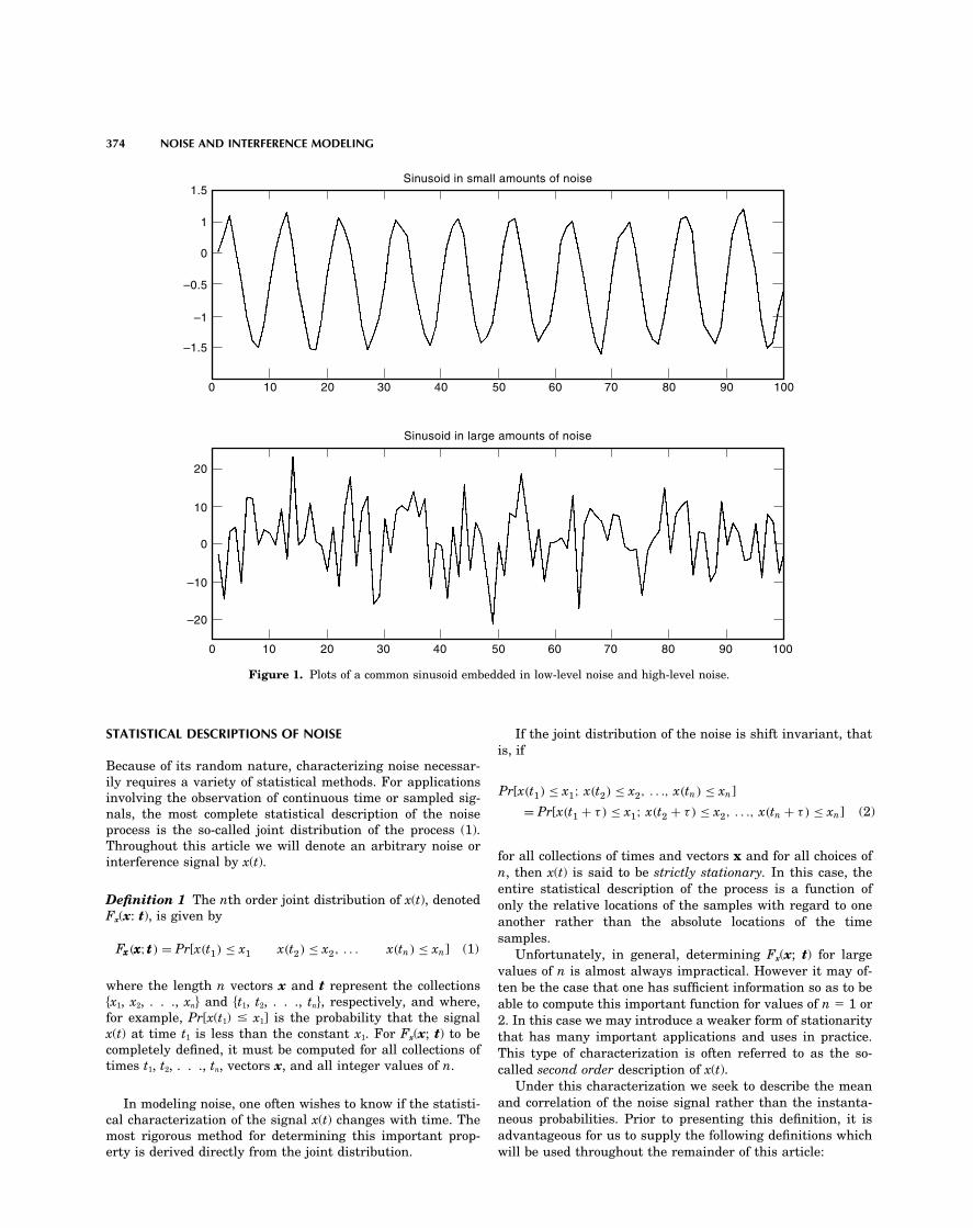
Unfortunately, it is more generally the case that the noiseand interference cannot be ignored. Rather, design and analy-sis must be done with careful attention to the corruptive ef-fects of these disturbances. One way to ensure an effectivefinal design is to have accurate models of the noise compo-nents of the signals of interest. Examples of the impact ofhigh and low levels of noise on the observation of a sinusoidare shown in Fig. 1.

Modeling these effects can range from being relativelystraightforward to being rather difficult if not impossible. Toassist in this endeavor, it is the purpose of this article to de-scribe various methods of characterizing noise and interfer-ence signals and to elaborate on some of the most popularmodels in practice today.

J. Webster (ed.), Wiley Encyclopedia of Electrical and Electronics Engineering. Copyright # 1999 John Wiley & Sons, Inc.

374 NOISE AND INTERFERENCE MODELING

0

0 10 20

Sinusoid in large amounts of noise

Sinusoid in small amounts of noise

30 40 50 60 70 80 90 100

10 20 30 40 50 60 70 80 90 100

1.5

1

0

–0.5

–1

–1.5

20

10

0

–10

–20

Figure 1. Plots of a common sinusoid embedded in low-level noise and high-level noise.

STATISTICAL DESCRIPTIONS OF NOISE If the joint distribution of the noise is shift invariant, thatis, if

Because of its random nature, characterizing noise necessar-ily requires a variety of statistical methods. For applicationsinvolving the observation of continuous time or sampled sig-nals, the most complete statistical description of the noise

Pr[x(t1) ≤ x1; x(t2) ≤ x2, . . ., x(tn) ≤ xn]

= Pr[x(t1 + τ ) ≤ x1; x(t2 + τ ) ≤ x2, . . ., x(tn + τ ) ≤ xn] (2)process is the so-called joint distribution of the process (1).Throughout this article we will denote an arbitrary noise or

for all collections of times and vectors x and for all choices ofinterference signal by x(t).n, then x(t) is said to be strictly stationary. In this case, theentire statistical description of the process is a function of

Definition 1 The nth order joint distribution of x(t), denoted only the relative locations of the samples with regard to oneFx(x: t), is given by another rather than the absolute locations of the time

samples.Fxxx(xxx;ttt) = Pr[x(t1) ≤ x1 x(t2) ≤ x2, . . . x(tn) ≤ xn] (1) Unfortunately, in general, determining Fx(x; t) for large

values of n is almost always impractical. However it may of-where the length n vectors x and t represent the collections ten be the case that one has sufficient information so as to be�x1, x2, . . ., xn� and �t1, t2, . . ., tn�, respectively, and where, able to compute this important function for values of n � 1 orfor example, Pr[x(t1) x1] is the probability that the signal 2. In this case we may introduce a weaker form of stationarityx(t) at time t1 is less than the constant x1. For Fx(x; t) to be that has many important applications and uses in practice.completely defined, it must be computed for all collections of This type of characterization is often referred to as the so-times t1, t2, . . ., tn, vectors x, and all integer values of n. called second order description of x(t).

Under this characterization we seek to describe the meanand correlation of the noise signal rather than the instanta-In modeling noise, one often wishes to know if the statisti-neous probabilities. Prior to presenting this definition, it iscal characterization of the signal x(t) changes with time. Theadvantageous for us to supply the following definitions whichmost rigorous method for determining this important prop-

erty is derived directly from the joint distribution. will be used throughout the remainder of this article:


Definition 2 The amplitude probability density function of Power Spectral Densitythe signal x(t) is given by

Engineers are often more comfortable in describing or analyz-ing signals in the frequency domain as opposed to the statisti-cal (or time) domain. This is equally true when dealing withrandom signals. However, random signals pose a few compli-

fx(x; t) = ∂Fxxx(x; t)∂x

for all choices of x and for all values of t (3)cations when one attempts to apply spectral techniques tothem. This is a consequence of the fact that each time onewhile the joint amplitude density function of x(t) is given bymakes an observation of this signal, the so-called noise real-ization (observation) is different and will therefore likely havea different spectrum. Moreover, many of these potential noiserealizations might have infinite energy, and will therefore not

fxxx(x1, x2; t1, t2) = ∂∂Fxxx(x1, x2; t1, t2)

∂x1∂x2

for all choices of x1 and x2 and for all t1 and t2 (4)have well-defined Fourier transforms.

Because of these complicating factors, we must considerThese two definitions completely characterize all of the first-the power spectrum (rather than the standard energy spec-and second-order properties of x(t) (e.g., mean values, signaltrum) averaged over all possible realizations to obtain aenergy and power, correlations and frequency content). Inmeaningful definition of the spectrum of a random signal.particular, the amplitude density function describes the sta-This approach leads to the well-known and oft-used powertistical range of amplitude values of signal x at time t. Fur-spectral density of the noise or interference as the basic fre-ther, one should recall from basic probability theory (2) thatquency domain description of x(t).the density functions f x(x; t) and f x(x1, x2; t1, t2) can be readily

To begin, assume that we only observe the noise signalobtained from the nth joint distribution of the signal x(t)x(t) from t � �T to t � �T (we will later let T approachgiven in Eq. (1) through simple limiting evaluations. Giveninfinity to allow for the observation of the entire signal). Thethese two density functions, we may define the second-orderFourier transform of this observed signal isdescription of the noise or interference signal as follows:

Definition 3 The mean or average value of the noise as afunction of time is defined as

XT (ω) =∫ T

−Tx(t)e− jωt dt (7)

We may then write the squared magnitude of XT(�) as follows:µx(t) = E[x(t)] (5)

where the expectation is taken with respect to f x(x; t). Thecorrelation function of the noise signal is defined as |XT (ω)|2 =

∫ T

−T

∫ T

−Tx(t1)x∗(t2)e− jω(t1−t2 ) dt1 dt2 (8)

Rx(t1, t2) = E[x(t1)x∗(t2)] (6) As described above, for the definition to have any utility,we need to compute the average magnitude squared powerand where the above expectation is taken with respect tospectrum, which requires that we must evaluate the expectedf x(x1, x2; t1, t2), and where x* denotes the complex conjugate ofvalue of �XT(�)�2 and then normalize this expectation by thex(t).length of the observation of x(t) (this prevents the spectrumfrom blowing up with power signals). This leads to the follow-If the mean function is a constant with respect to time (theing expression:average value of the noise does not change with time) and

the correlation function of the noise is a function of only thedifference of times and not their absolute locations, that is,Rx(t1, t2) � Rx(0, t2 � t1), then the noise is said to be wide-sensestationary. In this case we simplify the notation by letting themean be � and the correlation function be given by Rx(�)

12T

E[|XT (ω)|2] = 12T

∫ T

−T

∫ T

−TRx(t1 − t2) dt1 dt2 (9)

=∫ T

−T

[1 − |τ |

2T

]Rx(τ ) dτ (10)

where � � t2 � t1.A signal x(t) being wide-sense stationary implies that the where the second equation arises from a transformation of

average statistical properties as measured by the mean and variables. The final step in the definition is to allow the obser-the correlation function do not depend on when one observes vation window to grow to (��, ��), that is, to take the limitthe noise and interference. This is a very beneficial property of Eq. (10) as T tends to infinity. From this we arrive at thesince designers attempting to combat this noise are not re- following definition which holds for all wide sense stationaryquired to include an absolute clock in their design, rather a random signals.fixed design will always be optimal.

As an important observation, one should note that if the Definition 4 The power spectral density of a wide sense sta-noise happens to be strictly stationary then the noise will also tionary random signal x(t) is given bybe wide-sense stationary. This is a direct consequence of thefact that the mean and correlation functions are expected val-ues taken with respect to the first- and second-order joint

SX (ω) =∫ ∞

−∞Rx(τ )e− jωτ dτ (11)

density functions which, by supposition, are shift invariant.In general, the converse is not true. However, we will see Note that as a consequence of the preceding analysis, the

power spectral density turns out to simply be the Fourierlater that among the most popular models for the noise, thiswill, in fact, be the case. transform of the correlation function. Thus the correlation


function of a random signal contains all the information nec- where �(�) is the familiar Dirac delta function (3). Here oneshould observe from the above equation that white noise hasessary to compute the average spectrum of the signal and,

furthermore, there is a one-to-one relationship between the zero correlation between all time samples of the signal, nomatter how close the time samples are to one another. Thisaverage time dependency between samples (as measured by

the correlation function) and the average frequency content does not imply that all samples of white noise are indepen-dent from one another, rather that they simply have zero cor-in the signal.

The term ‘‘power spectral density’’ arises from the fact relation between them.Unfortunately, by integrating the power spectral densitythat SX(�) behaves like a probability density function. First,

just like a standard density function, it is always non-nega- over all frequencies we observe that the total power in whitenoise is infinite, which, of course, requires more energy thantive, and second, when integrated over a certain frequency

range one obtains the average power of the signal over that exists in the entire universe. Therefore, it is physically im-possible for white noise to exist in nature. Yet, there arefrequency range. That is, computing the integralmany noise processes which have essentially a constantpower spectral density over a fixed and finite frequencyrange of interest, which suggests that white noise may be

∫ −ω1

−ω2

SX (ω) dω +∫ ω2

ω1

SX (ω) dω (12)

an appropriate and simplifying model. Yet, the real utilityresults in the total power in the signal x(t) between the fre- of the white noise model is in describing other ‘‘nonwhite’’quencies �1 and �2 (Note: we must consider both positive and noise signals.negative frequencies.) This is just like the situation when one To demonstrate this, consider the output of a linear time-integrates a probability density function over a particular invariant system with frequency response H(�) to a whiterange to obtain the probability that the random variable will noise input. Under very general conditions, it can be shownfall into that range. (2) that this output, given by y(t), is a noise signal with power

Now given these few basic definitions, we may proceed to spectral density given bycharacterize various forms of noise or interference. From thestatistical perspective, what differentiates various types ofnoise are, first and foremost, the specific joint distribution of SY (ω) = N0

2|H(ω)|2 (15)

the process. Since these joint density functions are exceed-ingly difficult to obtain, we are often relegated to comparing Now, conversely, let us assume that we observe some non-and classifying noise signals through fX(x; t) and fX(x1, x2; t1, white noise signal with power spectral density SY(�). If � lnt2), as well as the mean and correlation function or power SY(�)/1 � �2 d� � ��, then y(t) can be modeled as the outputspectral density. of some linear time invariant system with a white noise input.

That is, there will exist some well-defined system with fre-quency response given by H(�) such that N0/2�H(�)�2 � SY(�).NOISE MODELSThese processes are, in fact, physically realizable and consti-tute all random signals seen in practice. Thus, from a spectralWhite Noiseperspective we may replace essentially all random signals

White noise is a model used to describe any noise or interfer-seen in nature by a linear system driven by a white noise

ing signal which has essentially equal power at all frequen-signal.

cies. More precisely, signals with a power spectral densitygiven by

Gaussian Noise

Gaussian noise is the most widely used model for noise orSX (ω) = N0

2for all frequencies (13)

interference both in practice and in the scientific literature.There are two primary reasons for this: (1) many observationsare said to be white because, similar to white light, these sig-in nature follow the Gaussian law, and (2) the Gaussian den-nals have equal power at all (visible) frequencies. Throughsity function is mathematically easy to analyze and manip-simple integration it is easily shown that the amount of powerulate.contained in white noise over an angular frequency range of

The reason that so many natural observations areB radians per second is N0B. (Note that the factor of 2 in theGaussian arises from the so-called Central Limit Theorem.definition of the power spectral density accounts for the two-This theorem is stated as follows:sided nature of the Fourier transform.)

It is important to note that this definition of white noise isnot an explicit function of either the amplitude density func- Theorem 1 Assume that Zi are independent, and identicallytion or the joint density function given in Eqs. (3) and (4), but distributed random variables, each with mean �Z and finiterather a function of only the power spectral density of the variance �2

Z. Then the so-called ‘‘normalized sum’’ given bysignal. Thus, any noise source, irrespective of the specificforms of fX(x; t) and fX(x1, x2; t1, t2) can be white noise, so longas the power spectral density is a constant. Yn

1√n

n−1∑i=1

Zi − µZ

σZ(16)

The corresponding correlation function of white noise is ob-tained through the inverse Fourier transform as

approaches a standard Gaussian random variable with meanequal to zero and unit variance, irrespective of the originaldistribution of the random variables Zi.

Rx(τ ) = N0

2δ(τ ) (14)


What this very powerful theorem establishes is that if a Now, let us extend this by considering the limiting casewhere the length of time between steps tends to zero (T � 0).particular observation of interest is a combination of infinitelyIt is easy to show that E[x2(nT)] � ns2 � ts2/T for t � nT. Tomany small and independent random components, then theensure that we do not have a variance going to zero (thecombination, when properly normalized, is Gaussian Randomwalker stops) or blowing up (not physically realizable), let usvariable with density function given byalso add the condition that the size of the step be proportionalto the square root of the time between steps, that is s2 � �T.Then the well-known Wiener Process is the signal x(t), which

fxxx(x; t) = 1√2π

e−x2/2 (17)

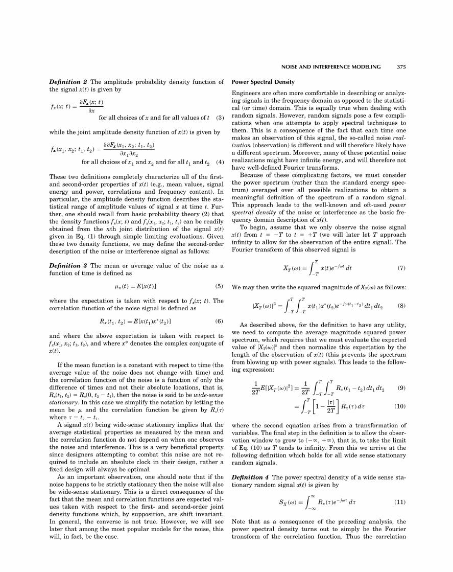
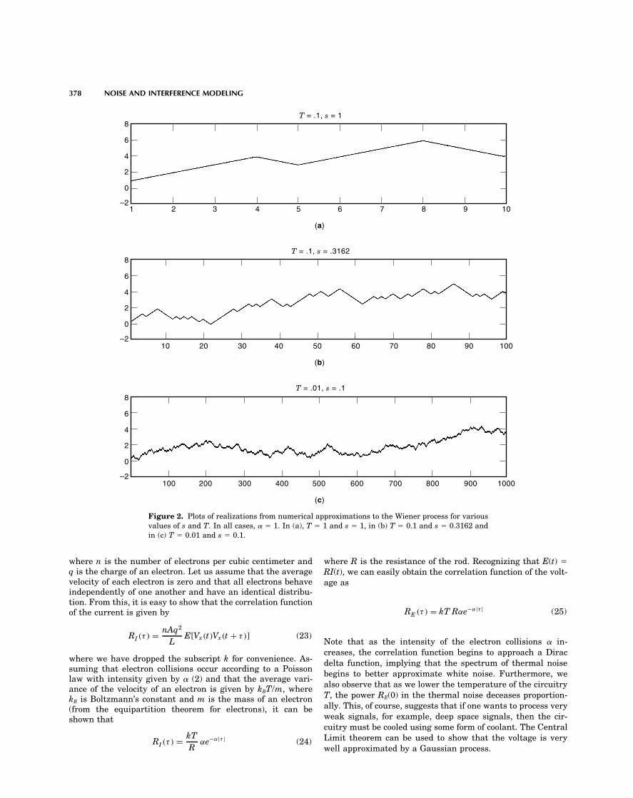
is the limit of the random walk under these conditions. Exam-ples of this are given in Fig. 2, where we have depicted real-This might suggest that all natural observations areizations from three succeeding approximations to the WienerGaussian since most physical phenomena are impacted byprocess. In all figures, we have let the proportionality con-many random events; however, extensive experimental re-stant � � 1. In Fig. 2(a) T and s equal 1, in Fig. 2(b) T � 0.1sults establish otherwise (4). Therefore, in addition to variousand s � �0.1, and in Fig. 2(c) T � 0.01 and s � 0.1. One canforms of Gaussian noise, later in this article we will presentsee that as the approximation gets closer to the limiting valuea number of other ‘‘non-Gaussian’’ noise models.it becomes smoother (more continuous) and begins to exhibitlong-term trends. This, of course, makes sense because theDefinition 5 A random noise signal is said to a Gaussiansteps are getting much smaller and, as a consequence, itsignal if all nth-order joint density functions are jointlytakes longer periods of time for the walker (signal) to changeGaussian, that is, if all joint density functions are of the formpositions (values).

It should be pointed out that as T � 0, the position of therandom walk at any point in time is the sum of infinitelyfxxx(xxx) = 1

(2π)n/2p

det(KKK)exp

[−1

2(xxx − µµµ)TKKK−1(xxx − µµµ)

](18)

many random steps, and therefore by the Central Limit Theo-rem, the location at any point in time is a Gaussian randomwhere the vector � and the matrix K represent the mean vec-variable with zero mean and variance given by �t.tor and covariance matrix (2), respectively, of the vector

To compute the correlation function of the Wiener process,x(t1), x(t2), . . ., x(tn). we note that x(t2) � x(t1) is independent of x(t1) due to the factthat, by supposition, the random movements between times

The important feature here is we see that for any value t1 and t2 are independent of the random movements up ton, the joint statistics of a Gaussian signal are completely de- time t1. From this it must be thattermined from the mean and correlation functions of x(t). Fur-thermore, when the signal is in addition wide-sense station- E[(x(t2) − x(t))x(t1)] = E[x(t2) − x(t1)]E[x(t1)] = 0 (20)ary, then the joint statistics are shift invariant, and as such,

from which it is easy to show that RX(t1, t2) � �t1 wheneverthe signal is also strictly stationary.t2 � t1. Determining the correlation for the case that t1 � t2Gaussian noise is further differentiated by the nature ofresults in the final value for the correlation function of thethe mean functions and the correlation functions. When theWiener process ascorrelation function is given by RX(�) � N0/2�(�), then the sig-

nal is said to be Gaussian White Noise, which is the singleRX (t1, t2) = α min(t1, t2) (21)most common model in noise analysis. In this case, each time

sample will be independent from all others and have infinite One can readily see that the Wiener process is not wide-sensevariance. Other well-known Gaussian models which we de- stationary and therefore does not have a computable powerscribe below are Wiener noise, Thermal noise, and Shot noise. spectral density. Nevertheless, it is a highly useful, physically

motivated model for Gaussian data with relatively smoothWiener Noise realizations and which exhibits long-term dependencies.

The Wiener Process is the limiting case of a random walkThermal Noisesignal. A random walk is a popular abstraction for describingThermal noise is one of the most important and ubiquitousthe distance an individual is from home when this individualsources of noise in electrical circuitry. It arises primarily fromrandomly steps forward or backward according to some proba-the random motion of electrons in a resistance and occurs inbility rule. The model is as follows: Every T seconds an indi-all electronic circuits not maintained at absolute zero degreesvidual will take a length s step forward with probability 1/2Kelvin. This resulting low-level noise is then scaled to sig-or a length s step backward with probability 1/2. Therefore,nificant levels by typical amplifiers used to amplify other low-at time nT, the position of the random walk will be x(nT) �level signals of interest.ks � (n � k)s, where n is the total number of steps taken, and

To derive a model for Thermal noise, let us assume thatk is the number of forward steps taken. For large values ofwe have a conducting rod of length L and cross-sectional areatime, it can be shown using the DeMoivre–Laplace TheoremA for which we expect to measure low-level random voltages.(2) thatLet Vx,k(t) denote the component of velocity in the x directionof the kth electron at time t. The total current denoted byI(t) is the sum of all electron currents in the x directionPr(x(nT ) = ks − (n − k)s) ≈ 1

pnπ/2

e−(2k−n)2/2n (19)

or that the location of the walker is governed approximatelyby a Gaussian law.

I(t) =nAL∑k=1

ik(t) =nAL∑k=1

qL

Vx,k(t) (22)


5 6 7 8 9 104321

T = .1, s = .3162

T = .1, s = 1

(a)

50 60 70 80 90 10030 402010

T = .01, s = .1

(b)

500 600 700 800 900 1000300 400200100

(c)

8

6

4

2

0

–2

8

6

4

2

0

–2

8

6

4

2

0

–2

Figure 2. Plots of realizations from numerical approximations to the Wiener process for variousvalues of s and T. In all cases, � � 1. In (a), T � 1 and s � 1, in (b) T � 0.1 and s � 0.3162 andin (c) T � 0.01 and s � 0.1.

where n is the number of electrons per cubic centimeter and where R is the resistance of the rod. Recognizing that E(t) �q is the charge of an electron. Let us assume that the average RI(t), we can easily obtain the correlation function of the volt-velocity of each electron is zero and that all electrons behave age asindependently of one another and have an identical distribu-tion. From this, it is easy to show that the correlation functionof the current is given by RE (τ ) = kT Rαe−α|τ | (25)

Note that as the intensity of the electron collisions � in-RI (τ ) = nAq2

LE[Vx(t)Vx(t + τ )] (23)

creases, the correlation function begins to approach a Diracwhere we have dropped the subscript k for convenience. As- delta function, implying that the spectrum of thermal noisesuming that electron collisions occur according to a Poisson begins to better approximate white noise. Furthermore, welaw with intensity given by � (2) and that the average vari-

also observe that as we lower the temperature of the circuitryance of the velocity of an electron is given by kBT/m, whereT, the power RE(0) in the thermal noise deceases proportion-kB is Boltzmann’s constant and m is the mass of an electronally. This, of course, suggests that if one wants to process very(from the equipartition theorem for electrons), it can beweak signals, for example, deep space signals, then the cir-shown thatcuitry must be cooled using some form of coolant. The CentralLimit theorem can be used to show that the voltage is verywell approximated by a Gaussian process.

RI (τ ) = kTR

αe−α|τ | (24)


Shot Noise

Shot noise is used to model random and spontaneous emis-sions from dynamical systems. These spontaneous emissionsare modeled as a collection of randomly located impulses(Dirac delta functions) given by z(t) � �i �(t � ti) where thelocations of the impulses in time (ti) are governed by a Poissonlaw with intensity � which is then driven through somesystem.

The output of a system with impulse response h(t) to theinput z(t) is said to be ‘‘shot noise.’’ From the convolution theo-rem, it is easily shown that this output is

x(t) =∑

i

h(t − ti) (26)

Using the properties of the Poisson law, is is easy to showthat the mean value of shot noise is �x � �H(0), where H(�)

0.8

0.7

0.6

0.5

0.4

0.3

0.2

0.1

–5 –4 –3 –2 –1 0 1 2 3 4 5

Laplacian

Gaussian

p = 5

p = 50

0

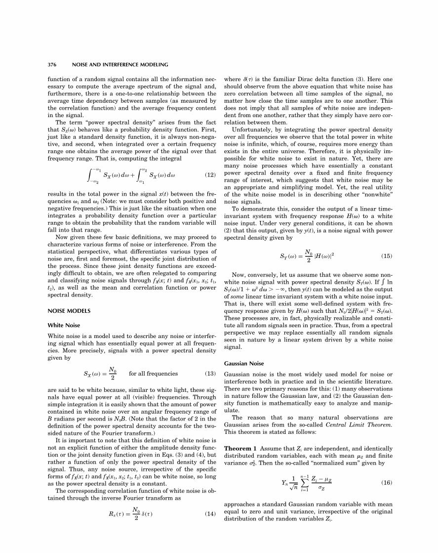
is the frequency response (Fourier Transform) of the system.Figure 3. Plots of various specific amplitude density functions fromThe power spectral density function of x(t) is given bythe Generalized Gaussian model.

SX (ω) = λ2H2(0)δ(ω) + λ|H(ω)|2 (27)

tails which decay to zero faster than the Gaussian tail giveThus the frequency content of the shot noise is determinedrise to data sets with fewer large values in the noise than oneentirely by the system h(t) and the intensity of the Poissonmight see with Gaussian data. On the other hand, when theprocess, that is, average rate of emissions. As before, becausetail of the amplitude density decays slower than that of thex(t) at large values of time is composed of the superpositionGaussian, one is more likely to see large random values of theof many random elements [see Eq. (26)] x(t) is often modelednoise signal x(t) than one would with Gaussian data. So, un-as a wide-sense stationary Gaussian random process withlike differentiating noise models based on the spectrum of thepower spectral density given by Eq. (27).noise, as seen in the preceding section, with non-Gaussiannoise we typically differentiate various forms by the nature of

NON-GAUSSIAN MODELS the tail of the amplitude density function.

While the scope of the Central Limit Theorem might suggest Generalized Gaussian Noiseotherwise, there are many data sets derived from the environ-

The Generalized Gaussian model is the most straightforwardment which do not conform well to the Gaussian model. Mostextension of the standard Gaussian model. In this case, theof these data contain interfering signals emitted from a mod-amplitude probability density function is given byest number of interferers or from interferers overlapping the

signal of interest in the frequency domain in such a way thatone could not easily remove these unwelcome elements by fil-tering.

fX (x; t) = a(p)exp�

−[ |x|

A(p)

]p�(28)

Approaches to remedy this modeling problem fall into twocategories: (1) generalize the Gaussian model to allow for sta- where the constant p parameterizes the density function and

where A(p) � �[�(1/p)/�(3/p)], a(p) � p/[2��(1/p)�A(p)] andtistical variation around the Gaussian process, or (2) attemptto derive new statistical models directly from the physics of where �(z) is the gamma function (generalized factorial). It

should be noted that, irrespective of the value of p, the vari-the problem. In both cases, most non-Gaussian specificationstypically do not go beyond the amplitude probability density ance of the amplitude density function is held constant (in

this case the variance is arbitrarily set to one). Plots of thefunction given in Eq. (3) and power spectral density. This isdue, in large part, to the severe complexity of merely speci- amplitude density function for p � 1, 2, 5, and 50 are depicted

in Fig. 3. One can see that for small values of (p 2), the tailsfying valid and useful joint probability functions with the de-sired amplitude density. of the density functions maintain relatively large values for

large arguments. Conversely, for large values of (p 2), theThese non-Gaussian models for noise and interference gen-erally differ statistically from Gaussian noise in the rate at tails decay to zero quite rapidly.

From Eq. (28), it is easily recognized that for p � 2, thewhich the so-called ‘‘tail’’ of the amplitude density tends tozero. More specifically, for Gaussian noise the amplitude Generalized Gaussian model results in a standard Gaussian

model. Alternatively, when p � 1, we obtain the well-knownprobability density function is approximated by e�x2/2�2 forlarge values of �x�. That is, the tails (the probability density Laplacian model for noise. In this case, the tail of the ampli-

tude density function decays at a rate of e��x�, thus implyingfunction from some large value to � infinity) of the amplitudedensity decay at an exponential rate with exponent equal to that one will likely observe many more large values of noise

than one would see with Gaussian noise. In general, forx2. From a physical point of view, this rate translates into therelative frequency of observing large amplitude values from p 2 we obtain tails with more mass (more probability), re-

sulting in ‘‘impulsive’’ data, while for p � 2 we obtain tailsthe noise signal. That is, amplitude density functions with


100500 200 150 200 250 350 400 450 500

Gaussian noise: p = 2

Laplacian noise: p = 15

0

–5

100500 200 150 200 250 350 400 450 500

Generalized Gaussian noise: p = 50

5

0

–5

100500 200 150 200 250 350 400 450 500

5

0

–5

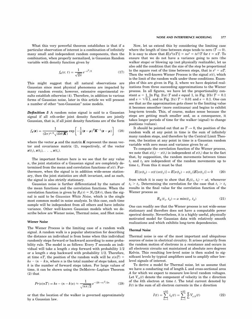
Figure 4. Plots of realizations from various density functions from the Generalized Gaussianfamily of density functions.

with less mass, resulting in data sets with very few outliers in the exponent of the characteristic function rather than theexponent of the amplitude density function (5).and more uniformly distributed over its range.

To demonstrate the variation in the data under this model,Fig. 4 shows sample realizations from Laplacian noise (p � Definition 6 A noise or interference signal is said to be an1), Gaussian noise (p � 2), and Generalized Gaussian noise �-sub Gaussian signal if for any positive integer n and timep � 50. One can see that these data sets, all with a common vector t � �t1, t2, . . ., tn�, the characteristic function of thevariance (power), exhibit quite different behavior. The Lapla- joint density function of [x(t1), x(t2), . . ., x(tn)] is given bycian noise better models interference which might containspikes such as those produced by man-made devices, whilep � 50 might better model interference arising from signalswith well-contained powers.

ϕ(uuu) = exp

�−

[12

n∑m,l=1

umulR(tm, tl )

]α/2�

(29)

where � � (1, 2] and where R(t, s) is a positive definite func-Sub-Gaussian Noisetion and where u � �u1, u2, . . ., un�.While in general one specifies a random signal through the

joint distribution function, sub-Gaussian noise is specified Importantly, if the parameter � � 2 then the sub-Gaussianprocess is simply a Gaussian process. Otherwise, the noisethrough the joint characteristic function (2). As a reminder,

this function is simply the Fourier transformation of the joint signal corresponds to some signal which has been parameter-ized away from the Gaussian signal. In all cases other thandensity function and, as such, there exists a straightforward

one-to-one relationship between characteristic functions and � � 2, the corresponding tail of the amplitude density func-tion decays at a polynomial rate (rather than an exponentialjoint density functions. As opposed to the Generalized

Gaussian noise model, sub-Gaussian noise is parameterized rate) which translates into many more very large amplitude


500 100 150 200 250

(a)

300 350 400 450 500

500 100 150 200 250

(b)

300 350 400 450 500

Sub-Gaussian noise: + 1.5

Sub-Gaussian noise: + 1.9915

10

5

0

–5

–10

20

15

10

5

0

–5

–10

–15

α

α

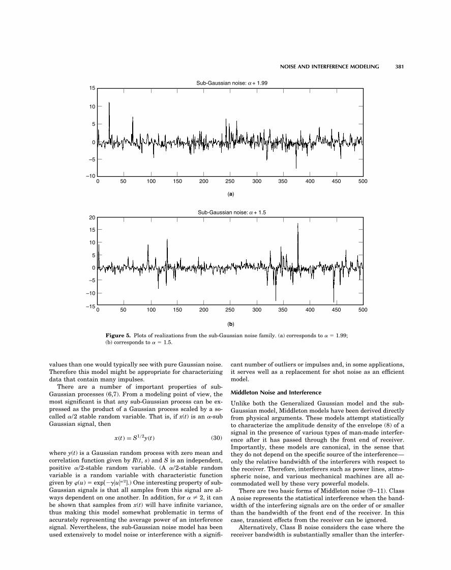
Figure 5. Plots of realizations from the sub-Gaussian noise family. (a) corresponds to � � 1.99;(b) corresponds to � � 1.5.

values than one would typically see with pure Gaussian noise. cant number of outliers or impulses and, in some applications,it serves well as a replacement for shot noise as an efficientTherefore this model might be appropriate for characterizingmodel.data that contain many impulses.

There are a number of important properties of sub-Middleton Noise and InterferenceGaussian processes (6,7). From a modeling point of view, the

most significant is that any sub-Gaussian process can be ex- Unlike both the Generalized Gaussian model and the sub-pressed as the product of a Gaussian process scaled by a so- Gaussian model, Middleton models have been derived directlycalled �/2 stable random variable. That is, if x(t) is an �-sub from physical arguments. These models attempt statisticallyGaussian signal, then to characterize the amplitude density of the envelope (8) of a

signal in the presence of various types of man-made interfer-ence after it has passed through the front end of receiver.x(t) = S1/2y(t) (30)Importantly, these models are canonical, in the sense that

where y(t) is a Gaussian random process with zero mean and they do not depend on the specific source of the interference—correlation function given by R(t, s) and S is an independent, only the relative bandwidth of the interferers with respect topositive �/2-stable random variable. (A �/2-stable random the receiver. Therefore, interferers such as power lines, atmo-variable is a random variable with characteristic function spheric noise, and various mechanical machines are all ac-given by �(u) � exp[��u��/2].) One interesting property of sub- commodated well by these very powerful models.Gaussian signals is that all samples from this signal are al- There are two basic forms of Middleton noise (9–11). Classways dependent on one another. In addition, for � � 2, it can A noise represents the statistical interference when the band-be shown that samples from x(t) will have infinite variance, width of the interfering signals are on the order of or smallerthus making this model somewhat problematic in terms of than the bandwidth of the front end of the receiver. In thisaccurately representing the average power of an interference case, transient effects from the receiver can be ignored.signal. Nevertheless, the sub-Gaussian noise model has been Alternatively, Class B noise considers the case where the

receiver bandwidth is substantially smaller than the interfer-used extensively to model noise or interference with a signifi-


ence bandwidth and thus transient effects must be accounted �-Mixture Noisefor. In addition to Class A and B noise, Middleton has intro-

One might observe from the above Middleton models that theduced the notion of Class C noise, which is simply a linear

amplitude density functions are infinite linear combinationscombination of both A and B noise (12).

of zero mean Gaussian models. Interestingly, it has been wellknown in the statistics literature that appropriately scaled

Physical Model. For both Class A and Class B noise, it is Gaussian density functions can be combined together to ob-assumed that there are an infinite number of potential tain nearly all valid amplitude density functions, so it is notsources of interference within reception distance of the re- surprising that this combination appears as a canonical rep-ceiver. The individual interfering signals are assumed to be resentation of signal interference.of a common form, except for such parameters as scale, dura- However, working with infinite sums of density functionstion, and frequency, among others. requires much careful analysis. It is because of this that re-

The locations and parameters of the interferers in the searchers have introduced a simplifying approximation to thesource field are assumed to be randomly distributed according Middleton Class A model, which is referred to as the �-mix-to the Poisson law. The emission times for each source are ture model.also assumed to be random and Poisson-distributed in time. In this simplification, the amplitude probability densityPhysically speaking, this implies that the sources are statisti- function of interference plus background or thermal noise iscally independent both in location and emission time. approximated by a combination of just two Gaussian density

functions:Class A Noise. As described above, the physical model for

Class A noise assumes that the bandwidth of the individualinterfering signals is smaller than the bandwidth of the re- fxxx(x; t) = (1 − ε)

1�2πσ 2

ε

e− x2

2σ 2ε + ε

1�2πγ σ 2

ε

e− x2

2γ σ 2ε (33)

ceiver (data-collection system.) This allows for the simplifica-tion of ignoring all transient effects (ringing) in the output of

where the constant � determines the fraction of impulsivitythe receiver front end.found in the data and where � represents the ratio of intensi-Avoiding the tedious analysis and simply stating the re-ties of the impulsive component to nominal ambient noise. Insult, the (approximate) amplitude probability density functionorder to maintain a fixed power level of �2 in the noise andunder these assumptions was shown by Middleton (9) to beinterference model for all choices of � and �, the parametersmust satisfy the following power constraint:

fxxx(x; t) = e−A∞∑

m=0

Am

m!1�

2πσ 2m

e− x2

2σ 2m (31)

σ 2ε = σ 2

1 − ε + εγ(34)

whereSample realizations from the �-mixture model are depicted

in Fig. 6. The top figure corresponds to purely Gaussian noise(� � 0), while the middle and bottom figures correspond toσ 2

m = m/A + �

1 + �and � = σ 2

G/ (32)

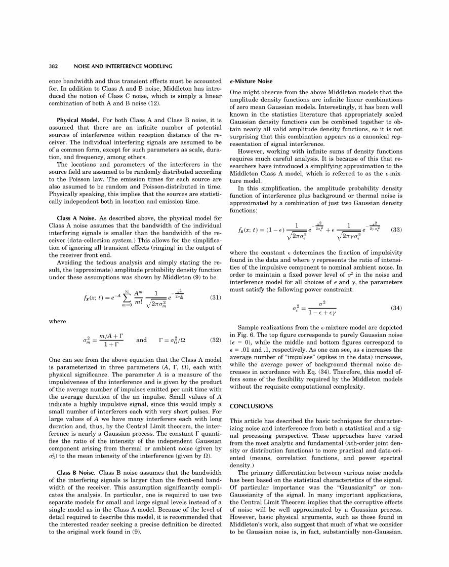
� � .01 and .1, respectively. As one can see, as � increases theaverage number of ‘‘impulses’’ (spikes in the data) increases,One can see from the above equation that the Class A modelwhile the average power of background thermal noise de-is parameterized in three parameters (A, �, ), each withcreases in accordance with Eq. (34). Therefore, this model of-physical significance. The parameter A is a measure of thefers some of the flexibility required by the Middleton modelsimpulsiveness of the interference and is given by the productwithout the requisite computational complexity.of the average number of impulses emitted per unit time with

the average duration of the an impulse. Small values of Aindicate a highly impulsive signal, since this would imply a CONCLUSIONSsmall number of interferers each with very short pulses. Forlarge values of A we have many interferers each with long This article has described the basic techniques for character-duration and, thus, by the Central Limit theorem, the inter- izing noise and interference from both a statistical and a sig-ference is nearly a Gaussian process. The constant � quanti- nal processing perspective. These approaches have variedfies the ratio of the intensity of the independent Gaussian from the most analytic and fundamental (nth-order joint den-component arising from thermal or ambient noise (given by sity or distribution functions) to more practical and data-ori-�2

G) to the mean intensity of the interference (given by ). ented (means, correlation functions, and power spectraldensity.)

The primary differentiation between various noise modelsClass B Noise. Class B noise assumes that the bandwidthof the interfering signals is larger than the front-end band- has been based on the statistical characteristics of the signal.

Of particular importance was the ‘‘Gaussianity’’ or non-width of the receiver. This assumption significantly compli-cates the analysis. In particular, one is required to use two Gaussianity of the signal. In many important applications,

the Central Limit Theorem implies that the corruptive effectsseparate models for small and large signal levels instead of asingle model as in the Class A model. Because of the level of of noise will be well approximated by a Gaussian process.

However, basic physical arguments, such as those found indetail required to describe this model, it is recommended thatthe interested reader seeking a precise definition be directed Middleton’s work, also suggest that much of what we consider

to be Gaussian noise is, in fact, substantially non-Gaussian.to the original work found in (9).


50 100 150 200 250 300 350 400 450 5000

50 100 150 200 250 300 350 400 450 5000

50 100 150 200 250 300 350 400 450 5000

(a)

(b)

(c)

= .01, = 100ε γ

= .1, = 100ε γ

= 0, = 100ε γ4

2

0

–2

–4

10

0

–10

–20

10

5

0

–5

–10

Figure 6. Plots of realizations from the �-mixture noise family. (a) corresponds to � � 0 (pureGaussian noise,) (b) corresponds to � � 0.01 (a 1% chance of observing interference at any pointin time) and (c) corresponds to � � .1 (a 10% chance of observing interference at any point intime.) One should observe that as � increases, the empirical frequency of ‘‘impulses’’ arising frominterference increases proportionally.

Moreover, it has been shown in much research that imposing BIBLIOGRAPHYthe Gaussian model on data which are decidedly or margin-

1. R. M. Gray and L. D. Davisson, Random Processes: A Mathemati-ally non-Gaussian can have detrimental effects on the finalcal Approach for Engineers, Englewood Cliffs, NJ: Prentice-Hall,designs. It is therefore critical that when one is dealing with1986.data, particularly arising from interfering sources, that the

2. A. Papoulis, Probability, Random Variables, and Stochastic Pro-appropriate model be used and used accurately.cesses, New York: McGraw-Hill, 1984.For readers interested in pursing these topics further, one

3. A. V. Oppenheim, A. S. Willsky, and I. T. Young, Signals andshould begin with the important original work found in (13). Systems, Englewood Cliffs, NJ: Prentice-Hall, 1983.Explicit models governing a wide variety of random phenom- 4. E. J. Wegman, S. C. Schwartz, and J. B. Thomas (eds.), Topics inena can be found in (14–16). For an advanced treatment of Non-Gaussian Signal Processing, New York: Springer-Verlag,random process in general, books by Doob (17) and Wong and 1989.Hajek (18) are excellent if not somewhat advanced treatments 5. C. L. Nikias and M. Shao, Signal Processing with Alpha-Stable

Distributions and Applications, New York: Wiley, 1995.of the theory of random signals.

384 NOISE GENERATORS

6. Y. Hosoya, Discrete-time stable processes and their certain prop-erties, Ann. Probabil., 6 (1): 94–105, 1978.

7. G. Miller, Properties of certain symmetric stable distribution. J.Multivariate Anal., 8: 346–360, 1978.

8. J. G. Proakis, Digital Communications, 3rd ed., New York:McGraw-Hill, 1995.

9. D. Middleton, Canonical non-gaussian noise models: Their impli-cation for measurement and for prediction of receiver perfor-mance, IEEE Trans. Electromagn. Compatibil., EMC-21: 209–220, 1979.

10. D. Middleton, Statistical-physical models of electromagnetic in-terference, IEEE Trans. Electromagn. Compatibil., EMC-19: 106–127, 1977.

11. D. Middleton, Procedures for determining the parameters of thefirst-order canonical models of class a and class b electromagneticinterference, IEEE Trans. Electromagn. Compatibil., EMC-21:190–208, 1979.

12. D. Middleton, First-order non-gaussian class c interference mod-els and their associated threshold detection algorithms, Tech.Rep. NTIA Contractor Rep. 87-39, Natl. Telecommun. Inf. Ad-ministration, 1987.

13. N. Wax, ed., Noise and Stochastic Processes, New York: Dover,1954.

14. N. L. Johnson, S. Kotz, and A. W. Kemp, Univariate Discrete Dis-tributions, 2nd ed., New York: Wiley, 1992.

15. N. L. Johnson and S. Kotz, Continuous Univariate Distributions,Vol. 1, Boston: Houghton-Mifflin, 1970.

16. N. L. Johnson and S. Kotz, Continuous Univariate Distributions,Vol. 2, Boston: Houghton-Mifflin, 1970.

17. J. L. Doob, Stochastic Processes, New York: Wiley, 1953.18. E. Wong and B. Hajek, Stochastic Processes in Engineering Sys-

tems, New York: Springer-Verlag, 1985.

GEOFFREY C. ORSAK

Southern Methodist University

NOISE, CIRCUIT. See CIRCUIT NOISE.

W3409

Documents

Transcript of W3409