I .

SLAC-PUB4498May 1994(A)

Developments in Electron Gun Simulation*

W. B. Herrmannsfeldt

Stanford Linear Accelerator Center

Stanford University, Stanford, CA 94309

ABSTRACT

This paper will discuss the developments in the electron gun simulation

programs that are based on EGUN and its derivatives and supporting programs.

Much of the code development has been inspired by technology changes in computer

hardware; the implications on EGN2 of this evolution will be discussed. Some

examples and a review of the capabilities of the EGUN family will be described.

Invited talk presented at the 6th International Symposium on Electron Beam

Ion Sources and Their Applications, Stockholm, Sweden, June 2&23, 1994.

* Work supported by Department of Energy contract DE–AC03–76SFO0515.-..

--

1

1. Introduction

Technological progress in the performance of small computers has rapidly

changed the demands on the software that is properly matched to the hardware.

Table I shows running times on some PC-clones and workstations for the electron

optics program EGN2e [1] running a simulation of the Electron Beam Ion Source

(EBIS) gun model EGUN84 [2].

The speed incre~es shown in Table I have been accompanied by a reduction

in memory cost that now permits from 8 to 32 MBYTE, or more of RAM in PCs.

The challenge for the supplier of a simulation code such as EGN2e, is to respond

to” the increasing computer capability and increasingly challenging demands by

users, in the way that best meets the needs of the community, while preserving the

investment in experience with the program. In this paper, we will describe how

EGN2e has been developed in response to these factors.

The original PL-1 and Fortran versions of EGUN for mainframe computers

have evolved into today’s family of programs including preprocessors, graphics

- programs, and post processors all working together in support of the C program

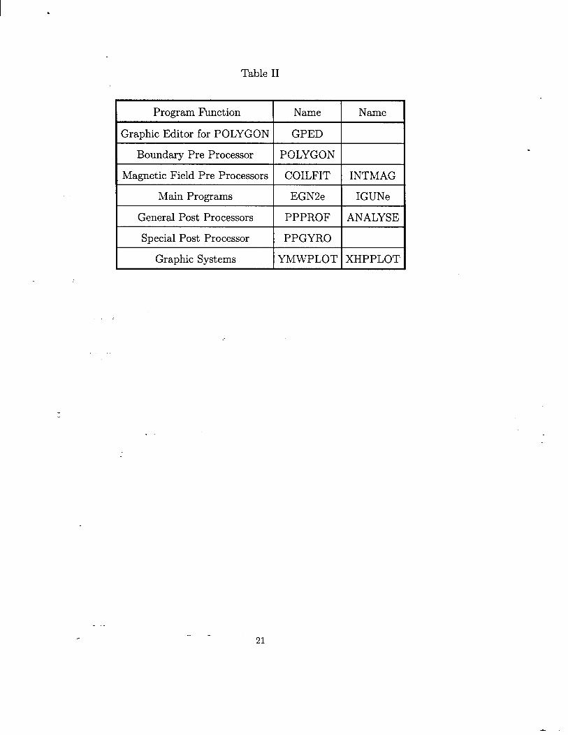
EGN2 and the Fortran program IGUNe. This family tree is illustrated in Table 11.

The most obvious result of the increase in computer speed for a mesh-based

program is that larger numbers of mesh points can be used while maintaining

reasonable computation time. Since the primary reason for using more mesh points

is to get better resolution and better accuracy, various steps must be taken to assure

that improved accuracy is in fact achieved. We will be considering the implications

of larger size problems in the following sections.

-..--

2

I .

2. Problem Size

The program EGN2 is written in the C language. One advantage of using

C is that it is relatively straightforward for the program to do internal array

allocations”. This is in contrmt to the program IGUN [3], the ion source program

written by Becker, which uses FORTRAN-77 and has fixed mrays determined

by the programmer. The extent to which the choice of array allocation method

matters to the user depends only on whether he/she can run problems with M many

mesh points and trajectories M are desired. Thus for example, by using suitable

compilers, both IGUN and EGN2e can be run in protected mode on a PC running

either DOS or 0S/2. EGN2e can also be run in ordinary DOS, m was done for

the

the

PC examples in Table I, using expanded memory for cases in which the size of

problem exceeds that allowed by the conventional 640 kBYTE RAM of DOS.

There are a number of different ways in which large numbers of mesh points

tiect the way a program operates. Some of these also tiect the user who must be

aware of possible pitfalls, of which perhaps the most obvious is that an adequate

solution of the potentials is found by the Laplace and Poisson equation solver.-.

More mesh points imply a solution time that can go up roughly with the square

of the number of points, but there are things that the user can do that will either

greatly speed up the convergence or conversely, can slow it down and even result

in it being unlikely that a good solution can be achieved. The two most obvious

steps that the user can take are:

1. Assist the program in having a good preload of the potential arrays, which

means that the initial filling of the potential array should be a reasonable

first guess for the final solution, and-..

--3.

I .

2. Obtain an adequate initial solution for Laplace’s Equation (before space

charge is added).

For a problem dominated by space charge, such as a space-charge-limited Pierce

diode, it is not necessary to have a very good Laplace solution before adding

space charge. Conversely, for a device without much space charge, such w a

photomultipliers tube or even a field emission diode, it maybe adequate to run only

one program cycle to get a self-consistent solution, so that a very good solution to

Laplace’s Equation is important, In EGN2 we have provided the parameter PASS,

m well ~ a modifier of the internal error criterion, ERROR, in the initial control

section of the program, to allow users to determine the number of “passes” to be

made of Laplace’s Equation.

The preload can be affected by the user who takes time to understand

the algorithm that we use to determine the initial potential distribution. We

interpolate potentials on each successive row of interior points from left to

right. Any boundary segment with a fixed potential forms an end point for the

interpolar ion. This means that a pair of parallel plates would have the initial

preload that is identical to the final correct solution. However, if a plate with a hole

leading to a long beam tunnel is used, this interpolation may result in the critical

central part of the problem area having a very bad solution. A concerned user can

resist the program by providing a surface of dummy boundary points on which

a suitable potential has been defined. Dummy boundary points are points which

do not define either a Dirichlet (metal) or Neumann boundary. Such a dummy

boundary segment will only affect the preload; used in this way it can easily speed

convergence by very large factors.-..

--4

-.

I .

Lmgeproblems imply large, complex boundary configurations. Fortunately the

boundary-definition-program POLYGON [4] by Reinard Becker is available to eme

the creation of boundary files. Recent versions of POLYGON can pms on all the

other control and initialization data needed by EGN2, so that users do not have to

repeatedly edit these files. POLYGON is provided with every copy of EGN2 and is

integrated within IGUN. The GRaphical Polygon EDitor (GPED) [5] is available

to trace the problem boundary on a computer screen as it is being defined.

The accuracy of the complete solution of Poisson’s equation depends also on

the way space charge has been deposited on the mesh nodes. A recent improvement

in EGN2 is to do space charge allocation the same way it is done in IGUN and in

various other programs such as Particle-in-Cell (PIC) codes; that is, by allocating

space -charge to the four nearest node points on every integration step. The

allocated charge is a product of the step time and the current in the trajectory. This

improvement in the space charge allocation has resulted in problems such a the

EGUN84, shown in Fig. 1, having a much more uniform distribution of trajectories.

The high-area convergence of EBIS guns like EGUN84 causes particles to pms

through the mesh at very steep angles. The new allocation algorithm deposits

space charge correctly for particles with any angle of inclination through the mesh.

.

-..--

5

3. Magnetic Fields

There are several significant are~ of development in EGN2e relating to

magnetic fields, including:

1.

2.

3.

Implementing equations of motion in XYZ coordinates

singularity on the axis for equations in R@Z coordinates,

to eliminate the

Making provision to store the scalar arrays of magnetic field components B.

and BZ on the same mesh m that used for the electric field solution.

Continuous development and support of the magnetic field simulation

program INTMAG [6] by Reinard Becker. INTMAG h= output formats

which are matched to the needs of EGN2e and IGUN.

Precise implementation of externally imposed magnetic fields is very important

in the correct simulation of the- matching conditions of guns with large ratios

of cathode area to find beam area. This condition applies to several clmses of

problems including especially linear beam microwave tubes and EBIS guns. In

- Figs. 2 and 3 we show the EBIS gun of Fig. 1, now with the imposed magnetic

field. The mismatched solution of Fig, 2 contrasts obviously with the well-matched

solution of Fig. 3. However, the differences in the external magnetic fields are not

so great. In fact, the same field solution, provided by INTMAG, is used in both

cases, but with a small longitudinal shift.

The beam’s

magnetic field.

trajectory path,

own self magnetic field is treated separately from the external

The particles are calculated through the entire length of the

one by one, starting from the axis and proceeding outward. In

a laminar beam, this mode of calculation allows the self-magnetic field to be

calculated for all the current that affects each successive ray. As the particles begin

-..--. 6

I .

to undergo non-laminar crossings, this method suffers in accuracy but is designed

to do so gradudly. Another accuracy problem results for intense relativistic beams,

where the self-magnetic field nearly exactly cancels the space chmge. The normal

mode of operation, in which space charge is calculated from the previous program

cycle and self-magnetic field is calculated from the present particle distribution,

can result in the taking of differences between two large forces of opposite sign from

successive cycles. The resulting errors can be quite large. A solution is suggested by

the fact that the residual defocusing force is very small, so that if the space charge

and self-magnetic field terms are subtracted directly, rather than by depositing the

full charge on the mesh, the program should converge. Because this method does

not correctly treat longitudinal space charge, which is what causes the emission

to be space charge limited, it is necessary to restrict its application to regions of

relativistic velocity. Thus in high=voltage devices, the parameter ZDOTEQ allows

the user to specify the relativistic velocity above which the calculation will be made

in the way described above, which is known as the EBQ mode. Typically a value

of ZDOTEQ of around 0.9 or so, would be used to cause the calculation to switch

to the EBQ mode. In an electron gun, the value of ZDOTEQ could reasonably be

chosen to correspond to the tunnel velocity.

The equations of motion derived in Ref. [1] include a conservation of angular

momentum term for ROZ coordinates. No particle with finite angular momentum,

or which is in a longitudinal magnetic field, can be allowed to pass through R = O

in such a coordinate system. However, because the integration is made in finite

steps, as the trajectory approaches the axis of symmetry, very small steps must be

taken to avoid the severe mathematical disaster that occurs by division by a very

small number. In fact, even for particles that do not approach the axis, this method-..

--. 7

I .

was found to give small errors in problems, such as for instance an electron beam

lithography system, in which a test problem consisted of mapping four emission

points to four target points in a uniform magnetic field. Most modern PIC codes

use XYZ coordinates, in which the axis is not a singularity, by resolving the radial

terms E. and B. into corresponding x and y components of the fields. Since the

integration must keep track of the azimuthal position of the trajectory anyway,

this does not add significantly to the amount of computation. The NAMELIST

input parameter CSYS=2 switches the program into the XYZ coordinate system.

However, all the input and output tables still show the cylindrical symmetry

formats, so that there is no overt sign that the program is operating with the XYZ

equations.

There. are several ways to input magnetic fields into EGN2e, M:

1. A polynomial expression for the axial field, B= = f(z), at R = O,

2. An array of values for B. at R = O,

3. A set of ideal point coils, or current loops, where the user specifies the R and

Z locations of the coils, and the current on each, and

4. A complete map of all the scalar field terms B. and B= on each mesh point

which-h~ been previously defined as interior points to the problem.

Method (4) above, is the most general but obviously depends on having output

from a suitable magnet design program. It replaces a capability that was in

earlier (FORTRAN) versions of EGUN, which could accept data from the program

POISSON for the vector potential A(r,z). In this new implementation, data from

any magnet design program can be taken as input, provided that the program can

save magnetic field data in a table so that the R and Z coordinates appear on a

line with values of B, and BZ. The EGN2e input routine can be directed to select

-..--. 8

--

I *

which columns represent which numbers even if other irrelevant data are on the

line. The significant factor which allowed this implementation is the availability

of extra memory in most small computers. Thus there is now allocated space in

the large ~rays for the magnetic field data. When the program reds in the file

of magnetic fields, it selects only those points which lie inside the boundaries of

the electrostatic problem. It is the responsibility of the user to ~sure that at least

that part of the problem area that is likely to have any pmticles is included

magnetic field data.

in the

Magnetic fields for Method (4) are calculated by simple interpolation of the

data for the four nearest mesh points. For all of the other three methods, the

normal way to calculate fields is by a sixth-order radial expansion of the axial

fields. -This method h~ proven remarkably accurate in the past. In the c~e of the

EGUN84 problem, for example, the same results are found by either the full map

or by “the off-axis expansion. However, there are some constraints on this method

that users must consider:

(a) The data must have full double-precision accuracy for the sixth-order

differences to be calculated. This is internally controlled if method (1) or

(3) is used, but if the user provides an array of field data for method (2),

he must be aware that crude data, such N from a magnetic me~urement

probe, cannot be used directly. (Such data can however be used in one

of the methods described below. )

(b) Expansions cannot go past magnetic elements, such as the point coils.

(c) As mesh density is incre=ed, the off-axis expansion may be asked to

extend farther in the radial direction (by a ratio to the bme of 13 mesh

points along the =is), and thus ultimately to introduce significant errors.-..

-.9

—-

I .

Although such errors have not been observed, this is the new factor that

results from larger mesh areas, and is the one factor that inspired the

provision of the full map of scalar arrays.

The generally preferred method among the choices 1) to 4) above, is number

3), sets of ideal point coils. There are three distinct advantages to this approach:

(a)

(b)

(c)

The data sets are the most compact.

Fields can be found anywhere in space, not just in the region near the

axis, by using the elliptic integral formulas which are internal to the

program. The elliptic functions provide exact solutions for the magnetic

fields from a set of coils. Although these routines are rather slow for

most ray-tracing applications, they can be used m an option for cases

in which off-axis expansions are not appropriate. An example of such a

c~e is one in which the solenoid is used to defocus a beam which p=ses

outside of the solenoid coils.

By using both the elliptic integrals and the off-wis expansion method,

EGN2 provides a table of field values which can be used to compare

the accuracy of the off-axis expansions. This table is provided for any

use of the point coils. The user provides a parameter RMAG which

determines the radius at which the comparison is to be made. Typically

RMAG is set to approximate the outer radius of the beam in the region

of strongest magnetic field focusing. RMAG has no other implications

besides providing the diagnostic table of magnetic fields.

We do not usually recommend using method 1), the polynomial expression

for the axial field, with the exception that a simple one-term expression is the

easiest way to specify a magnetic field that is uniform over the whole problem area.-..

--. 10

—.

.

Other polynomial expressions will generally not be consistent with any feasible

configuration of magnetic elements, and thus will result in very non-physical off-uis

fields.

There are two ways in which magnetic field data that lacks full double precision

accuracy can still be used:

(a) The less satisfactory way is simply to reduce the extent of the power

series used to calculate off-axis fields. This series can be reduced to

either second or fourth order in R. The field terms for BZ are even, and

the terms for B. are odd, so that the highest order term is always a BZ

term. The variable MAGORD determines the extent of the power series.

The better way to use data that does not have the proper precision

is with a program that can find a set of ideal point coils that closely

approximates the desired field. The program COILFIT does this by

making a least squares fit to the input data. The user specifies

number of point coils (less than the number of data points) and

desired radial and axial positions of the coils. COILFIT finds

the

the

the

currents on the coils to fit the desired data, and then can fill in the entire

p~oblem length with fields calculated from the ideal coils, to full double

precision. Alternatively, the user can choose the coil data to input into

EGN2, thereby preserving the other noted advantages of using the ideal

point coils. COILFIT is available as a preprocessor program for EGN2.

-..-.

11

—.

I .

4. Other Capabilities

As noted e~lier, the EGUN family of programs includes several pre and

post-processor programs. We briefly touched on the preprocessors above.

The main program EGN2e has, as was noted, a companion program IGUN for

the specific purpose of ion extraction from a gaseous pl~ma. IGUN can do the

pmticle ray tracing, including space charge and other effects, just as EGN2e does.

There are two general-purpose post-processor programs, PPPROF and

ANALYSE. They differ mostly in that PPPROF was written to take data from

a binary file of records of the particle trajectories, while ANALYSE extracts its

information from the space charge map in the printed output file. They also differ in

that ANALYSE was developed by the Frankfurt group, and PPPROF is a product

of the SLAC group. Both have the objective of providing beam profile information

as a function of Z. Each EGN2e simulation concludes with the usual ray tracing

plot and with phase spxe and beam profile plots, PPPROF extends the diagnostic

information that appears with the final results to an arbitrary number of locations

along the =is.

Special purpose post-processor routines can be developed to read and interpret

the binary file. One which has filled a special need is PPGYRO for examining data

from a gyrotron beam. Here the objective of the designer is to impart the maximum

angular velocity to the beam while maintaining beam quality, meaning especially

that particles should all be close together in azimuthal ph~e. The diagnostic

expressions in PPGYRO evaluate the results for each location in Z.

Many electron guns, including especially those which, like the EBIS gun,

have large area convergence ratios, are limited in the final beam spot size by-..

--. 12

I .

the transverse temperature of the particles. The limiting small value of this

temperature is the cathode temperature, typically around 0.1 eV. EGN2e accepts

the beam temperature in degrees-kelvin and calculates a radial energy increment

to be added and subtracted from particles that start from the initial coordinates of

each “ideal” particle, i.e., before adding the thermal energy. There are three models

using 2, 3, and 5 particles, respectively, for each initial particle. The tw~particle

model is the most satisfwtory because it includes a random-number generator to

give a statistical sense to the process.

of

in

For someone not experienced with thermal effects, the initial transverse energy

0.1 eV may sound negligible. However, radial compression of the beam results

a proportional incre~e in the temperature. This temperature increase is a

direct consequence of Liouville’s theorem and is not influenced by beam intensity.

Space charge forces, which are typically non-linear for a red distribution, are an

additional heating mechanism. The measure of all these effects is the beam phme

space which EGN2e calculates in several

“ b~es of 4 times the rms emittance to get

sometimes known w the 9570 emittance.

ways. The calculation is made on the

the effect of the beam edge emittance,

It is frequently desirable to be able to

then can be computed sequentially. EGN2e

segment a problem into parts which

creates an input data set for the final

conditions of the particles in the format that the program needs. This data can be

saved directly in a designated file, or it can be extracted from the output listing.

Sometimes it is useful to have the initial condition data in the same format, so

this is included in the above file. The problem scale and initial Z location of the

particles can be shifted by the parameters SKAL and ZO.-..

--. 13

—-

I &

There are also cmes in which it is desired to make changes in the first segment

of a simulation and see how the beam is affected in later stages. In such cases,

dl the segments can be placed together in the input stream, with the parameter

SAVE=2 signdling that input ray data should be t~en from the previous problem.

The same SKAL and ZO parameters apply in this case.

A variation

of one solution

together in the

indicating that

of saved data is when the boundaries and potential distributions

are desired for subsequent runs. Again the problems are placed

input stream, with the parameter SAVE= 1 in the first data set

the next one should not read boundaries and should not clear

the potential and space charge arrays. One possible application of this capability

might be for a long drifting beam, again like the EBIS simulation, in which both

the particles and the boundaries might be saved. Another example would be an

examination of the trajectories of secondary and scattered particles. The particles

can be initialized from chosen locations and traced in a configuration that includes

the spxe-charge fields from the first part. This capability can be useful for

simulating particles coming from a beam collector, for example, or from electrodes

in an accelerating column.

The PC:versions of the EGUN family all use the YMWPLOT program which

makes screen images on all standard combinations of monitors and graphics boards.

YMWPLOT also has the capability to make accurate, high-resolution, hard copy

renditions of the results by creating and sending a bitmap image of the figure to

either “laserjet” or dot-matrix printers. This approach is far superior to a screen

dump which is limited to screen resolution, and usually does not work anyway for

graphic images.

needs, all make-..

.

EGN2e, and the other members of the EGUN family with plotting

a file of the type *.cpl. It is this file that is read by YMWPLOT,

--14

I .

The *.cpl files can also be read by the program XHPPLOT which wm developed

to make plots on pen plotters using the Hewlett-Pachd HPGL graphics language.

XHPPLOT has recently been enhanced to make “postscript” files that can be used

by word processors and for making plots on UNIX systems.

5. Miscellaneous Applications

Although EGN2 was, as the name implies, developed for

designing electron guns, it has been used to simulate numerous

devices, some quite interesting and worthy of mention.

the purpose of

other electronic

It hm always been possible to include dielectric materials in EGUN simulations,

but recently this capability has been enhanced by the inclusion of special potential

numbers that EGN2 interprets as dielectric coefficients. This substantially reduces

the work required to create a data file for a problem which includes dielectrics.

We reported on simulations of field emitters at the Toulouse conference on

Charged Particle Optics [7]. This capability has found increasing application to

~ the new field of microelectronics. The resolution needed to simulate field emitters

may be as small-as 1 angstrom, as it was for the simulation of a small bump on

the tip of ti emitter of 200 angstrom radius shown in Fig. 4. Since the density of

mesh points increases by the square of the magnification, it is easy to see that a

faster computer with larger memory, makes only a small difference in the allowed

resolution. The configuration that ended with the simulation shown in Fig. 4

began with a 500 angstrom resolution simulation of a gated field emitter. The

most important thing is to reduce the area that must be simulated by finding

suitable boundary conditions. The boundary input processor POLYGON accepts

equipotential line and field line coordinates from EGN2 and uses these lines m-..

--. 15

I .

boundaries fora magnified problem. Typically, magnifications byafactorof5to

10 can be used; but two or even three magnifications may be needed to get the

required resolution. Three magnifications were used to achieve the final 500 times

magnification shown in this example.

Figure 5 shows a simulation of

is deployed on the Swedish Freja

designed by Whalen, et al. [8] at

is an electrostatic analyzer for the

the ~eja F3C Cold Plasma Analyzer which

Satellite. The Cold Plasma Analyzer was

the National Research Council, Canada. It

detection and study of ionospheric charged

particle distributions in the range 0.0 < E/Q < 200 eV, where E/Q is energy

per unit charge. The device is cylindrically symmetric, but the incoming particle

flux hm a large angular acceptance range so that understanding the angular and

momentum resolution is a major comput ation project. The Cold Plasma Analyzer

is an interesting example of a device other than a gun that can be studied with

an electron gun program; EGN2e will be used for simulations to determine the

resolution and acceptance of the instruments.

Acknowledgments

The C programming for EGN2 and all of the graphics support have been the

work of Glen A. Herrmannsfeldt. The boundary preprocessor POLYGON and

the magnetic field preprocessor INTMAG, and much of the inspiration for making

the improvements discussed here was been provided by Reinard Becker. We thank

them for their assistance in assembling the material for this paper and especially for

their many contributions to the EGUN family of programs. We are also indebted

to support from colleagues at SLAC and for suggestions and encouragement from

the significant user community of the EGUN programs.

-... --

16

I .

REFERENCES

[I] Herrmannsfeldt, W. B., EGUN-An Electron Optics and Gun Design Program,

SLAC–Report-331, Stanford Linear Accelerator Center, 1988.

[2] Becker, R., Kleinond, M., Thomae, H,, and Donets, E. G., Proc. HCI-92, ed.

Richard, P., Stockli, M., Cocke, C.L., andLin, C.D., AIP Conf. Proc. 686

(1993).

[3] Becker, R.and Herrmannsfeldt, W. B.,lGUN-A program ~orthe simulation

of positive ion etiraction including magnetic fields, RSI 63, April 1992

(2756).

[4] Becker, R., Easy Bounda~ Definition for EGUN, Nuclear Inst. Meth. B42

162-164 (1989).

[5] Zipfer, B. and Kester, O., Graphic Editor for Polygon, private communication

‘(1993).

[6] Becker, R., INTMAG, A Program for the Calculation of Magnetic Fields by

Integration Nuclear Inst. Meth. B42 303-306 (1989).

[7] Herrmanns~eldt, W. B., Becker, R., Brodie, I., Rosengreen, A., and Spindt,

C., High-Resolution Simulation of Field Emission, Third International

Conference on Charged Particle Optics, Toulouse, Prance, Nuclear Inst.

Meth. A298 39-44 (1990).

/8] Whalen, B. A., et al., The Freja F3C Cold Plasma Analyzer, Space Science

Journal, to be published.

-..--

17

I .

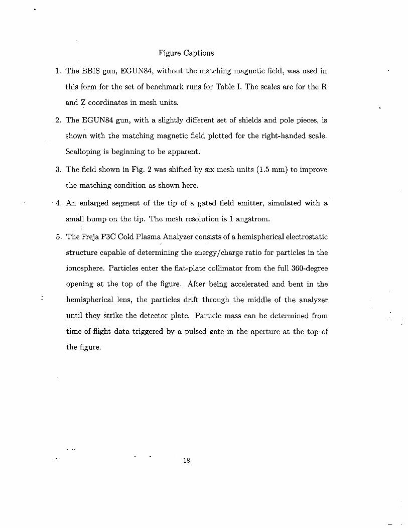
1. The EBIS gun, EGUN84,

Figure Captions

without the matching magnetic field, was used in

this form for the set of benchmark runs for Table I. The scales are for the R

and Z coordinates in mesh units.

2. The EGUN84 gun, with a slightly different set of shields and pole pieces, is

shown with the matching magnetic field plotted for the right-handed scale.

Scalloping is beginning to be apparent.

3. The field shown in Fig. 2 was shifted by six mesh units (1.5 mm) to improve

the matching condition as shown here.

4. An enlarged segment of the tip of a gated field emitter, simulated with a

small bump on the tip. The mesh resolution is 1 angstrom.

5. The Reja F3C Cold Plasma Analyzer consists of a hemispherical electrostatic

structure capable of determining the energy/charge ratio for particles in the

ionosphere. Particles enter the flat-plate collimator from the full 360-degree

opening at the top of the figure. After being accelerated and bent in the

hemispherical lens, the particles drift through the middle of the analyzer

until they ;trike the detector plate. Particle mass can be determined from

time-of-flight data triggered by a pulsed gate in the aperture at the top of

the figure.

-..--

18

Table Captions

Table I: EGN2e Running Times for the EBIS Gun, EGUN84.

Table II. The EGUN Family.

-..

. --19

—-

I .

Table I

Computer System* Compiler* EGUN84 (see)

80286, 8 MHz, DOS MS C-7.O 4990

80386, 25 MHz, DOS MS C-7.O 685

SUN, IPC Sun OS 4.1.3 128

80486, 66 MHz, DOS I MS C-7.O I 108

80486, 66 MHz, 0S/2 Borland 0S/2 59.3

RS/6000, 320 H, AIX XL C-1.2 51.5

Pentium, 66 MHz, DOS I MS C-7.O I 49.7

Pentium, 60 MHz, 0S/2 Borland 0S/2 31.8

RS/6000, 580, AIX XL C-1.2 13.5

DEC ALPHA, 200 MHz OSF/1 12.5

RS/6000, 590, AIX I XL C-1.2 I 7.0

* The identifiers in the above table are, of course, all registered trademarks.

-..--

20

.

Table II

(

Program Function Name Name

Graphic Editor for POLYGON GPED

Boundary Pre Processor POLYGON

Magnetic Field Pre Processors COILFIT INTMAG

Main Programs EGN2e IGUNe

General Post Processors PPPROF ANALYSE

Special Post Processor PPGYRO

Graphic Systems YMWPLOT XHPPLOT

-..--

21

.

-..

I I I

—

L

1

/1

m 0 m 0w R

—e

--

0

Fig. 1

.

-..--

T!mN

L

.

\

\

—

o

om

Fig. 2

.

-..

. --

TtmN

\

Fig. 3

II

n-.Q.

72

48

24

0

5-94

,!

1

I I I

I

o 48 96 144 1927664A4

I .

150

120

-90

60

30

0

-’/

o5-94

-..

30 60 90 1207684A5

Fig. 5