Vytautas Valancius, Cristian Lumezanu, Nick Feamster, Ramesh
26
Vytautas Valancius , Cristian Lumezanu, Nick Feamster, Ramesh Johari, and Vijay V. Vazirani
Transcript of Vytautas Valancius, Cristian Lumezanu, Nick Feamster, Ramesh

Vytautas Valancius, Cristian Lumezanu, Nick Feamster, Ramesh Johari, and Vijay V. Vazirani

Blended rate: Single price in $/Mbps/month
Charged each month on aggregate throughput Some flows are costly Some are cheaper to serve Price is set to recover total costs +
margin
Convenient for ISPs and clients
2
Cogent
EU Cost: $$$
US Cost: $
Blended rate Price: $$
GaTech
Can be inefficient!

3
Uniform price yet diverse resource costs
Lack of incentives to conserve resources to costly destinations
Lack of incentives to invest in resources to costly destinations
Pareto inefficient resource allocation A well studied concept in economics
Potential loss to ISP profit and client surplus
Clients ISPs
Alternative: tiered pricing

Some ISPs already use tiered pricing Paid peering Backplane peering Regional pricing Limited number of tiers
4
Price the flows based on cost and demand
Cogent
Global, Cost: $$$
Local Cost: $
GaTech
Regional pricing example:
Price: $$$
Price: $
Question: How efficient is such tiered pricing? Can ISPs benefit from more tiers?

1. Construct an ISP profit model that accounts for: Traffic demand of different flows Servicing costs of different traffic flows
3. Drive the model with real data Demand functions from real traffic data Servicing costs from real topology data
4. Test the effects of tiered pricing!
5
How can we test the effects of tiered pricing on ISP profits?
Modeling
Data mapping
Number crunching

Flow revenue Price * Traffic Demand Traffic Demand is a function of price How do we model and discover demand functions?
Flow cost Servicing Cost * Traffic Demand Servicing Cost is a function of distance How do we model and discover servicing costs?
6
Profit = Revenue – Costs (for all flows)
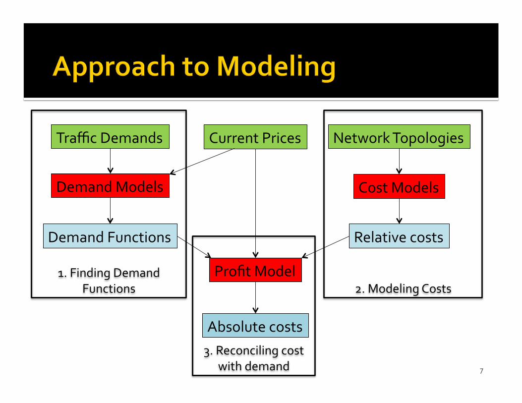
1. Finding Demand Functions
3. Reconciling cost with demand
2. Modeling Costs
7
Traffic Demands Network Topologies Current Prices
Demand Models
Demand Functions
Cost Models
Relative costs
Profit Model
Absolute costs

8
Demand = F(Price, Valuation, Elasticity)
Valuation = F‐1(Price, Demand, Elasticity)
Canonical commodity demand function: Price
Demand
Elastic demand
Inelastic demand
Valuation – how valuable flow is Elasticity – how fast demand changes with price
Current price
Current flow demand
Assumed range of elasticities
We mapped traffic data to demand functions!
How to find the demand function parameters?

1. Finding Demand Functions 2. Modeling Costs
9
Traffic Demands Network Topologies Current Prices
Demand Models
Demand Functions
Cost Models
Relative costs
Profit Model
Absolute costs

10
Linear: Concave:
Region: Dest. type:
How can we model flow costs?
ISP topologies and peering information alone can only provide us with relative flow servicing costs.
real_costs = γ * relative_costs

1. Finding Demand Functions
3. Reconciling cost with demand
2. Modeling Costs
11
Traffic Demands Network Topologies Current Prices
Demand Models
Demand Functions
Cost Models
Relative costs
Profit Model
Absolute costs

12
Data mapping is complete: we know demands and costs! Subject to the noise that is inherent in any structural estimation.
Profit = Revenue – Costs = F(price, valuations, elasticities, real_costs)
F’(price*, valuations, elasticities, real_costs) = 0
F’ (price*, valuations, elasticities, γ * relative_costs) = 0
γ = F’‐1(price*, valuations, elasticities, relative_costs)
Assuming ISP is rational and profit maximizing:

1. Select a number of pricing tiers to test 1, 2, 3, etc.
2. Map flows into pricing tiers Optimal mapping and mapping heuristics
3. Find profit maximizing price for each pricing tier and compute the profit
13
Repeat above for: ‐ 2x demand models ‐ 4x cost models ‐ 3x network topologies and traffic matrices

14 *Elasticity – 1.1, base cost – 20%, seed price ‐ $20
Constant elasticity demand with linear cost model
Tier 1: Local traffic Tier 2: The rest of the traffic

15
Linear Cost Model Concave Cost Model
Constant Elasticity Demand
Logit Demand
Having more than 2‐3 pricing tiers adds only marginal benefit to the ISP
The results hold for wide range of scenarios Different demand and cost models Different network topologies and demands Large range of input parameters
Current transit pricing strategies are close to optimal!
16
Questions? http://valas.gtnoise.net

17

Very hard to model!
Perhaps requires game‐theoretic approach and more data (such as where the topologies overlap, etc.)
It is possible to model some effects of competition by treating demand functions as representing residual instead of inherent demand. See Perloff’s “Microeconomics” pages 243‐246 for discussion about residual demand.
18

19

1. Past 4‐5 tiers the costs are marginal in practice (Section 5.)
2. Higher costs with more tiers reinforce our findings: more tiers will add even less benefit to ISP.
20

ISPs can perfect these models to estimate how much different flows add to their cost structure.
ISPs can use the pricing methods we developed.
ISPs can verify if, given their topology and demand, they might benefit form more tiers.
21

Some ISPs already use tiered pricing Backplane peering ▪ Charge less for traffic you can offload to peers in the same PoP
Paid peering and on‐net/off‐net pricing ▪ Charge less for on‐net traffic
Regional pricing ▪ Charge less for local traffic
22
Price flows based on cost and demand
How is such pricing implemented?

Detail how tiered pricing done Explain that paper is not about this Paper is about how many tiers is wise to have
Explain implications to operators: If few tiers are enough then we’re all set If many tiers are good, then look forward at implementing them. Perhaps also look forward to some granular bandwidth market (think enron)
23

Here is why we see the result
24

If demand is concentrated, a few tiers will add a lot of benefit.
For the rest of demand, depends on cost. Marginal cost differences ‐> marginal gain in profit with many tiers
Large cost differences ‐> tangible gain in profit with many tiers
25

We don’t know elasticities, so we test large range of them.
The data might be biased already for the traffic because of congestion signalling (maybe demand is more than we see).
We can’t model competition long term (no one can)
26