VVImp Missing Values v14

Missing Values Imputation

A New Approach to Missing Values Processing with Bayesian Networks

Stefan Conrady, [email protected]

Dr. Lionel Jouffe, [email protected]

December 19, 2011

Conrady Applied Science, LLC - Bayesia’s North American Partner for Sales and Consulting

mailto:[email protected]




Table of Contents

Introduction

Motivation & Objective 4

Overview 5

Notation 5

Theory of Missing Values Processing

Types of Missingness 6

Methods for the Analysis of Incomplete Data 8

Ad Hoc Methods 8

Listwise Deletion 8

Pairwise Deletion 8

Imputation 8

Single Mean Imputation 8

Conditional Mean Imputation 9

Multiple Imputation (MI) 9

Ad Hoc Methods Summary 9

Maximum Likelihood Estimation (ML) 10

Bayesian Networks 10

Missing Values Processing in Practice

Linear Example 12

Data Generating Process (DGP) 12

Missing Data Mechanism (MDM) 13

Standard Methods 14

Listwise/Casewise Deletion 14

Pairwise Deletion 14

Single Mean Imputation 15

Multiple Imputation (MI) 15

Missing Values Processing with Bayesian Networks 17

Static Completion 18

Dynamic Completion 19

Missing Values Imputation with Bayesian Networks

www.conradyscience.com | www.bayesia.com ii

http://www.conradyscience.com


http://www.bayesia.com


Nonlinear Example 23

Data Generating Process (DGP) 23

Bayesian Network Representation 24

Missing Data Mechanism 26

Bayesian Network Learning & Missing Values Imputation 28

Unsupervised Learning 28

Imputation 30

Summary Nonlinear Example 31

Summary & Outlook 31

Appendix

About the Authors 32

Stefan Conrady 32

Lionel Jouffe 32

References 33

Contact Information 35

Conrady Applied Science, LLC 35

Bayesia S.A.S. 35

Copyright 35


www.conradyscience.com | www.bayesia.com iii





Introduction

Motivation & Objective

With the abundance of “big data” in the field of analytics, and all the challenges today’s immense data vol-ume is causing, it may not be particularly fashionable or pressing to discuss missing values. After all, who cares about missing data points when there are petabytes of more observations out there?

As the objective of any data gathering process is to gain knowledge about a domain, missing values are ob-viously undesirable. A missing datum does without a doubt reduce our knowledge about any individual ob-servation, but implications for our understanding of the whole domain may not be so obvious, especially when there seems to be an endless supply of data.

Missing values are encountered in virtually all real-world data collection processes. Missing values could be the result of non-responses in surveys, poor record-keeping, server outages, attrition in longitudinal surveys or the faulty sensors of a measuring device, etc. What’s often overlooked is that not properly handling miss-ing observations can lead to misleading interpretations or create a false sense of confidence in one’s findings, regardless of how many more complete observations might be available.

Despite the intuitive nature of this problem, and the fact that almost all quantitative studies are affected by it, applied researchers have given it remarkably little attention in practice. Burton and Altman (2004) state this predicament very forcefully in the context of cancer research: “We are concerned that very few authors have considered the impact of missing covariate data; it seems that missing data is generally either not rec-ognized as an issue or considered a nuisance that it is best hidden.”

As missing values processing (beyond the naïve ad-hoc approaches) can be a demanding task, both method-ologically and computationally, the principal objective of this paper is to propose a new and hopefully eas-ier approach by employing Bayesian networks. It is not our intention to open the proverbial “new can of worms”, and thus distract researchers from their principal study focus, but rather we want to demonstrate that Bayesian networks can reliably, efficiently and intuitively integrate missing values processing into the main research task.


www.conradyscience.com | www.bayesia.com 4





Overview

1. We will first provide a brief introduction to missing values and highlight a selection of methods that have been traditionally used to deal with this problem.

2. We will then use a linear and a nonlinear example to illustrate the different statistical methods and in-troduce missing values imputation with Bayesian networks.

Notation

To clearly distinguish between natural language, software-specific functions and example-specific variable names, the following notation is used:

• Bayesian network and BayesiaLab-specific functions, keywords, commands, etc., are capitalized and shown in bold type.

• Names of attributes, variables, nodes and are italicized.







Theory of Missing Values Processing

Missing values are deceiving, as they all appear the same, namely as null values in one’s dataset. Metaphori-cally speaking, they are like a colorless and odorless gas, invisible to the naked eye and undetectable by ol-faction, and thus seemingly immaterial. Yet we know from physics and chemistry that dangerous substances can be cloaked in an ethereal appearance.

While we want to focus on this paper how to practically deal with missing values, using a minimum of mathematical notation and statistical jargon, we need to introduce a few basic concepts that are essential for understanding the problem of missing values. We will keep this theory to a minimum and rather refer the interested reader to specialist literature for further study.

Types of Missingness

There are several types of missing data that are typically encountered in studies:

• First, data can be “Missing Completely at Random (MCAR)”, which requires that the missingness1 is completely unrelated to the data. More formally, this can be stated as:

p(R∣Yobs ,Ymis ,X,φ) = p(R∣φ)

where R is the missing data indicator and 𝜙 is a parameter that characterizes the relationship between R and the data. This implies that R does not depend on Yobs and Ymis, i.e. the observed and the missing parts of the data, or any covariates X.When data are MCAR, missing cases are no different than non-missing cases, in terms of the analysis be-ing performed. Thus, these cases can be thought of as randomly missing from the data and the only real penalty in failing to account for missing data is loss of power in any parameter estimation. Unfortunately, MCAR is a very strong assumption and generally not testable. As a result, analysts can rarely rely on this fairly benign condition.

• Secondly, data can be Missing at Random (MAR), which is a weaker assumption. For MAR data, the missingness depends on known values and is thus described fully by variables observed in the data set. This also means that R, which denotes the missingness of Y, is unrelated to the values of Ymis:

p(R∣Yobs ,Ymis ,X,φ) = p(R∣Yobs ,X,φ)

For instance, if MAR holds, one can regress Yobs on X for the respondents and then use this relationship to obtain imputed values for Ymis for the non-respondents (Shafer and Olson, 1998)For illustration we use an example from missingdata.org.uk: “…suppose we seek to collect data on in-come and property tax band. Typically, those with higher incomes may be less willing to reveal them. Thus, a simple average of incomes from respondents will be downwardly biased. However, now suppose we have everyone’s property tax band, and given property tax band non-response to the income question



1 It is important to note the difference between “missingness of a variable” and a “missing value.” “Missingness” refers

to the probability of not being observed, whereas “missing” refers to the state of not being observed.





is random. Then, the income data is missing at random; the reason, or mechanism, for it being missing depends on property band. Given property band, missingness does not depend on income itself.”

• Data can be missing in an unmeasured fashion, termed “nonignorable”, also called “Missing Not at Ran-dom” (MNAR) and “Not Missing at Random” (NMAR). This is the most general case, which includes all possible associations between missingness and data.

p(R∣Yobs ,Ymis ,X,φ)

Since the missing data depends on events or items which the researcher has not measured, such as the missing values Ymis themselves, this creates a challenge. A hypothetical example for this situation would a behavioral survey. Individuals who are engaging in dangerous behaviors may be less likely to “admit” the high-risk nature of their conduct and thus decline to respond. In comparison, “low-risk” respondents may quite willingly make statements with regard to their “safe” behavior.

• Filtered or Censored ValuesAt this point we should briefly mention a fourth type of missingness, which is less often mentioned in the

literature. We refer to it as “filtered values.” These are values that cannot exist, but often appear in data-sets as no different than other missing values that do exist, but have not been observed.

For instance, in an auto buyer survey, a question about rear-seat legroom cannot be answered by the owner of a two-seat roadster. Conceptually, these filtered values are similar to MAR values, they depend

on other variables in the dataset, e.g. given that vehicle type=roadster, rear seat legroom=FV. As opposed to MAR values, and as this example suggests, filtered values are determined by logic.

It is particularly important that these missing variables are not imputed with any estimated values, as a bias is highly likely. Rather, a new state, e.g. a code like “FV”, has to be added as an additional state to

the affected variables.2 The filtered value declaration can typically be done in the context of the ETL3 process, prior to the start of any modeling work. Upon definition of these filtered values, the “normal”

missing values processing can begin.



2 BayesiaLab provides a framework for dealing with such filtered values, so these filtered values are specifically not

taken into account while machine-learning a model of the data generating process. Furthermore, BayesiaLab excludes filtered values when computing correlations, etc.

3 ETL stands for “extract, transform and load”, referring to the data preprocessing prior to starting a statistical analysis.





Methods for the Analysis of Incomplete Data

We now want to provide a very brief and admittedly incomplete (no pun intended) overview of some of the common methods for dealing with incomplete data, although some of them must be used with great caution or may not even be recommended at all.

Ad Hoc Methods

Listwise Deletion

Given that many statistical estimations require a complete set of observations, any records with missing val-ues are often excluded by default from such computations. The first consequence is an immediate loss of samples, which may have been very costly to acquire. This (often rather involuntarily applied) method is known more formally as “listwise deletion” or “casewise deletion.” In the best case, an estimation on a re-duced set of observations may only increase the standard error, which is the case with MCAR data, but un-der different circumstances listwise deletion could bias the parameter estimates, which can be the case with MAR data. In situations when no case is completely observed, i.e. there is at least one missing value per set of observation records, listwise deletion is obviously not applicable at all.

Pairwise Deletion

To address the loss of data that is inherent in listwise deletion, pairwise deletion uses different data sets for the estimation of each parameter. For instance, pairwise deletion is used when a different subsets of com-plete data are used to compute each cell in a correlation matrix. One concern is the fact the separate compu-tation of variances on subsets can lead to correlation values exceeding plus or minus 1. Another issue is the absence of a consistent sample base, which leads to problems in calculating standard errors of estimated parameters.

Imputation

As opposed to deletion-type methods, we now want to consider the “opposite” approach, i.e. filling in the blanks with “imputed” values. Here, imputing means replacing the non-observed values with reasonable estimates, in order to facilitate the analysis of the whole domain. Upon imputation, complete case statistical methods can be used to estimate parameters, etc. Although it may sound like “statistical alchemy” to create values for non-existing datums, it can be appropriate to do so.

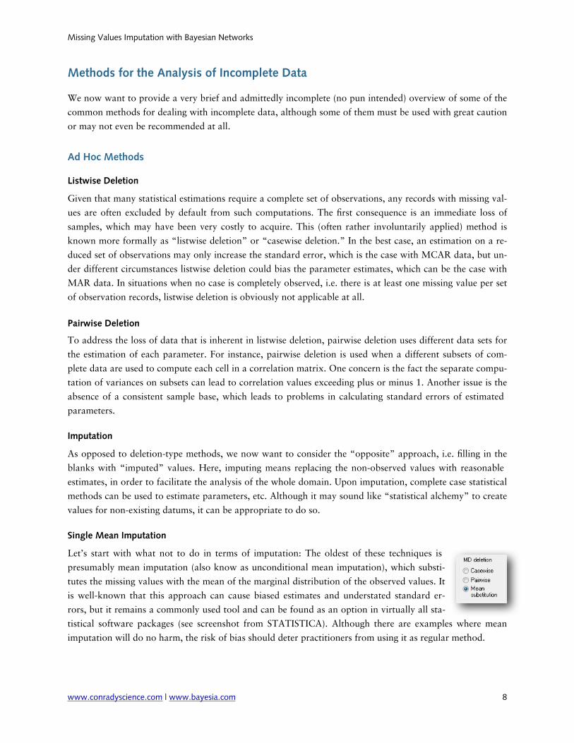
Single Mean Imputation

Let’s start with what not to do in terms of imputation: The oldest of these techniques is presumably mean imputation (also know as unconditional mean imputation), which substi-tutes the missing values with the mean of the marginal distribution of the observed values. It is well-known that this approach can cause biased estimates and understated standard er-rors, but it remains a commonly used tool and can be found as an option in virtually all sta-tistical software packages (see screenshot from STATISTICA). Although there are examples where mean imputation will do no harm, the risk of bias should deter practitioners from using it as regular method.







Conditional Mean Imputation

Conditional mean imputation (sometimes referred to as regression imputation) is a somewhat more sophis-ticated approach. If the MAR conditions are met, conditional mean imputation consists of modeling the missing values as a function of the observed values, such as with a regression. In effect, this method predicts the missing values from the observed values. However, in the case of a dataset with many variables that contain missing values, the specification of such functions can be a challenging endeavor in its own right. Shaffer (1997) states, “When the pattern of missingness is complex, devising an ad hoc imputation scheme that preserves important aspects of the joint distribution can be a daunting task.”

Assuming that this can be done successfully, one key issue remains for imputation methods that generate single values. Whenever a missing data point is imputed with a fixed value, it removes the uncertainty about the unknown variable, which inevitably results in underestimated errors. Even if the relationships can be adequately modeled, Shafer warns, “it may be a serious mistake to treat the imputed data as if they were real. Standard errors, p-values and other measures of uncertainty calculated by standard complete-data methods could be misleading because they fail to reflect any uncertainty due to missing data.” Intuitively, missing values should always increase standard errors due to the additional noise introduced by the miss-ingness and not reduce them.

While at the population level this lack of uncertainty may generate underestimated errors, for the individual records it does provide an optimal prediction of the missing values. However, as most studies are studying population-level effects, the predicted state of individual records may generally be of less relevance.

Multiple Imputation (MI)

To address the problem of determinism in conditional mean imputation, multiple imputation “reintro-duces” the uncertainty, as the name implies, by repeating the imputation multiple times. Multiple imputa-tion draws from a plausible distribution and thus generates the desired variance in the imputed values and in the subsequently computed parameter estimates. “Plausible distribution” also implies that the chosen imputation model is compatible with the functional form of the overall model of interest. For instance, if the overall relationship of interest is to be modeled with a linear regression, it would be suitable to also use a linear regression for the imputation model. Shafer and Olson (1998) provide a comprehensive overview of multiple imputation from a data analyst’s perspective.

The principles of MI were first proposed by Rubin in the 1970s, and even today MI remains a state-of-the-art method for missing values processing. Despite the undisputed benefits of this technique, it is not as widely used as one might expect (van Buuren, 2007).

Ad Hoc Methods Summary

All of the above imputation methods have in common that they create a complete dataset (or multiple com-plete sets, in the case of multiple imputation), so that the analyst can proceed with traditional estimation methods. Despite the proven, practical performance of these methods, there are perhaps two conceptual challenges that always add a degree of complexity to the research workflow:

1. The missing values imputation model is distinct from the statistical model that is meant to describe the domain’s overall characteristics, which should normally be at the core of the analyst’s efforts. This re-







quires, beyond the main model, a second set of assumptions regarding the functional form and the distri-butions.

2. For any imputation, special steps must be taken to reestablish the very uncertainty that is inherent in the absence of values.

Maximum Likelihood Estimation (ML)

The previous methods are all removing unknown values, either by means of deletion or imputation, prior to estimating the unknown parameters of the main model. This means that we treat unknown values as a sepa-rate (and often less important) problem versus the unknown parameters of a model. Schafer (1998) phrased the challenge as follows: “If we knew the missing values, then estimating the model parameters would be straightforward. Similarly, if we knew the parameters of the data model, then it would be possible to obtain unbiased predictions for the missing values.” The idea is of Maximum Likelihood (ML) estimation is to “merge” both unknowns into a single process and facilitate the estimation of the entire parametric model. We will not go into further details of the implementation of this approach, but we will later pick up the general idea of “jointly” estimating unknown values and unknown parameters with Dynamic Completion (Expectation-Maximization). A very comprehensive explanation of maximum likelihood estimation is pro-vided in Enders (2010).

Bayesian Networks

It goes beyond the scope of this paper to formally introduce Bayesian networks. Even a very superficial in-troduction would amount to a substantial portion of the paper, perhaps distracting from the focus on the missing values methods. For a very short and general overview we suggest our white paper, Introduction to Bayesian Networks (Conrady and Jouffe, 2011), for a much more comprehensive introduction, Bayesian Reasoning and Machine Learning (Barber, 2011) is highly recommended.

For dealing with incomplete datasets, Bayesian networks provide advantages that specifically relate to the two points stated in the summary of the ad hoc methods:

1. Bayesian networks offer a unified framework for representing the joint distribution of the overall domain and simultaneously encoding the dependencies with the missing values (Heckerman, 2008). This implic-itly addresses the requirement that Shafer and Olson stipulate for MI, namely “any association that may prove important in subsequent analysis should be present in the imputation model…. A rich imputation model that preserves a large number of associations is desirable because it may be used for a variety of post-imputation analyses.” Also, by using a Bayesian network, the “functional form” for missing values imputation and for representing the overall model are automatically identical and thus compatible.4

2. The inherently probabilistic nature of Bayesian networks allows to deal with missing values and their imputation non-deterministically. That means that the (needed) variance in the imputed data does not need to be generated artificially, but is inherently available.



4 In our case, the presented Bayesian network approach is nonparametric, so the term “functional form” is used loosely.





Using the terminology from the ad hoc methods, one could say that Bayesian networks can perform a kind of “stochastic conditional imputation.” Like all other previously mentioned imputation methods, the impu-tation approach with Bayesian networks also makes the MAR assumption.

An important caveat regarding the interpretation of Bayesian networks must be stated up front: In this pa-per, Bayesian networks are employed entirely non-parametrically. While this will provide many advantages that we will see in the subsequent examples, formal statistical properties cannot be established. Rather, the imputation performance of Bayesian networks and the BayesiaLab software can only be established through empirical tests and simulation.







Missing Values Processing in Practice

We will now illustrate several traditional methods for missing values processing as well as the relatively new approach of using Bayesian networks for that purpose. To facilitate a comparison of methods, we start with a linear example and then later explore a nonlinear case, which provides fewer options for the researcher.

Linear Example

Data Generating Process (DGP)

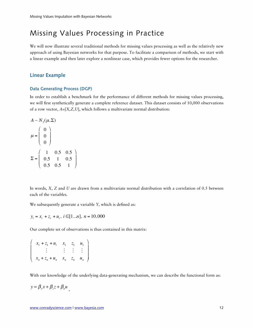
In order to establish a benchmark for the performance of different methods for missing values processing, we will first synthetically generate a complete reference dataset. This dataset consists of 10,000 observations of a row vector, A=[X,Z,U], which follows a multivariate normal distribution:

A N3(µ,Σ)

µ =000

⎛

⎝

⎜⎜

⎞

⎠

⎟⎟

Σ =1 0.5 0.50.5 1 0.50.5 0.5 1

⎛

⎝

⎜⎜

⎞

⎠

⎟⎟

In words, X, Z and U are drawn from a multivariate normal distribution with a correlation of 0.5 between each of the variables.

We subsequently generate a variable Y, which is defined as:

yi = xi + zi + ui , i ∈[1...n], n = 10,000

Our complete set of observations is thus contained in this matrix:

x1 + z1 + ui x1 z1 u1

xn + zn + un xn zn un

⎛

⎝

⎜⎜⎜

⎞

⎠

⎟⎟⎟

With our knowledge of the underlying data-generating mechanism, we can describe the functional form as:

y = βxx + βzz + βuu ,







with the known parameters βx = βz = βu = 1

In our subsequent analysis we will treat these parameters as unknown and compute estimates for them from the manipulated dataset, i.e. once it was subjected to the Missing Data Mechanism.

Missing Data Mechanism (MDM)

In order to simulate a real-world situation, we now cause portions of X, Z and U from the original refer-ence dataset to be missing. More specifically, we will apply the following arbitrary rules:

P(xi = missing) = 1− 11+ eyi

,

P(zi = missing) = 1− 11+ e− yi

,

P(ui = missing) = 0 if xi= missing and yi= missingelse 1

⎧⎨⎪

⎩⎪

⎫⎬⎪

⎭⎪

In words, we apply a logistic function each for X and Z to generate the probability of missingness as a func-tion of the values of Y. This also means that the missingness of X (or Z) does not depend on values of X (or Z). This is a key condition for making the MAR assumption.

The choice of the logistic function (see graph) is arbitrary, but one could think of a lifestyle survey with Body Mass Index (BMI) as a target variable (Y). It is plausible that those with a “good” BMI are more likely to report details of their healthy lifestyle than those with a “poor” BMI and a presumably unhealthy lifestyle, hence the increasing probability of missing data points one the “poor” side of the scale.

-10 -5 5 10y

0.2

0.4

0.6

0.8

1.0

PHmissingL

More specifically, this means that with increasing values of Y (the independent variable), the probability of X (a dependent variable) missing is increasing (red curve), while the opposite is true for Z (blue curve).







Furthermore, the (also arbitrary) rule for U implies that U is always missing when both X and Z are ob-served. For instance, the variable U could represent a follow-up question in a survey that is only being asked when X and/or Z are item non-responses. Whatever the reason, with this rule characterizing the missing data mechanism we will never have a full set of observations for Y, X, Z and U.

The following table shows the first 20 observations once the MDM is applied.

Y X Z U0.503 )0.319 0.991)0.988 )2.1360.783 0.333 )0.4611.058 0.642 0.1780.646 0.923 0.4852.279 2.176 0.1340.380 0.413 0.228)0.647 )0.490 )0.4003.297 0.681 1.3171.871 0.603 0.6620.749 0.7012.266 )0.058 0.8542.762 0.696 1.0031.804 0.264 0.3200.110 0.749 0.130)0.273 0.851 )0.7181.526 0.271 0.351)1.873 )1.342 0.024)1.932 )0.563 )1.2092.206 )0.163 0.506

In total, this amounts to 50% of the X and Z data points missing and approximately 13% of U.

Standard Methods

First we will approach this dataset with traditional missing value processing methods. Estimating the regres-sion parameters and comparing them to the true known parameters will allow us to assess the performance of these methods.

Listwise/Casewise Deletion

With no complete set of observations available, listwise deletion is obviously not an option here. After delet-ing all cases with missing values, not a single case would be left in our dataset. In the case of a large number of variables in a study, this situation is not at all unrealistic.

Pairwise Deletion

With listwise deletion not being an option, pairwise deletion will be examined next. For the Y-X pair, we have 5,047 observations, for Y-Z and Y-U, we have 5,010 and 8,630 valid observations pairs respectively. We estimate the parameters with OLS and obtain the following coefficients:

βx = 1.529βz = 1.585βu = 1.419Constant = - 0.020







Clearly, the parameter estimates are quite different from the known values. More interestingly, and as sug-gested in the introduction, the computed value of R2=1.29 is not meaningful. As such, we do not gain much insight from this approach.

Single Mean Imputation

As an alternative to deletion methods, most statistics programs do have mean imputation available as the next option, so we will try this approach here. As a result, each (observed) variables’ mean values are im-puted to replace the missing values. Given that the MDM is not symmetric for X and Z, the mean of these observed variables is no longer zero:

µx = −0.524µz = 0.519µu = −0.001

When performing the regression on the basis of the mean-imputed values, we obtain the following parame-ters (standard errors are reported in parentheses):

βx = 1.187 (0.018)βz = 1.201 (0.019)βu = 1.784 (0.012)Constant = 0.001 (0.017)

Knowing the true parameters, i.e. βx = βz = βu = 1 , we can conclude that these parameter estimates from

the mean imputation are biased. So, the mean imputation does not successfully address the problem of miss-ing values here, as we had already suggested to in the introduction.

Multiple Imputation (MI)

Today, multiple imputation, is becoming widely available in statistical software packages, even though ref-erences to this method still remain relatively rare in applied research.

In any case, multiple imputation has very appealing theoretical and practical properties. Without spelling out the details of the computation, we will simply show the results from the MI function implemented in SPSS 20.







The pooled parameter estimates turn out to be very close to the true parameter values, far better than what was estimated with the pairwise deletion and the means imputation:

βx = 0.958 (0.007)βz = 0.957 (0.013)βu = 1.015 (0.009)Constant = -0.028 (0.013)

SPSS automatically computed a small value for the intercept, which was not included in our DGP function specification, but the overall performance is still very good and far ahead of the mean imputation.







Missing Values Processing with Bayesian Networks

In comparison to the very brief overview of some of the standard methods in the previous chapter, we will now provide a greater amount of detail as we discuss missing values processing with Bayesian networks and, more specifically, BayesiaLab. As readers will presumably be less familiar with this approach, we will present the workflow tutorial-style and illustrate it with screenshots when appropriate.

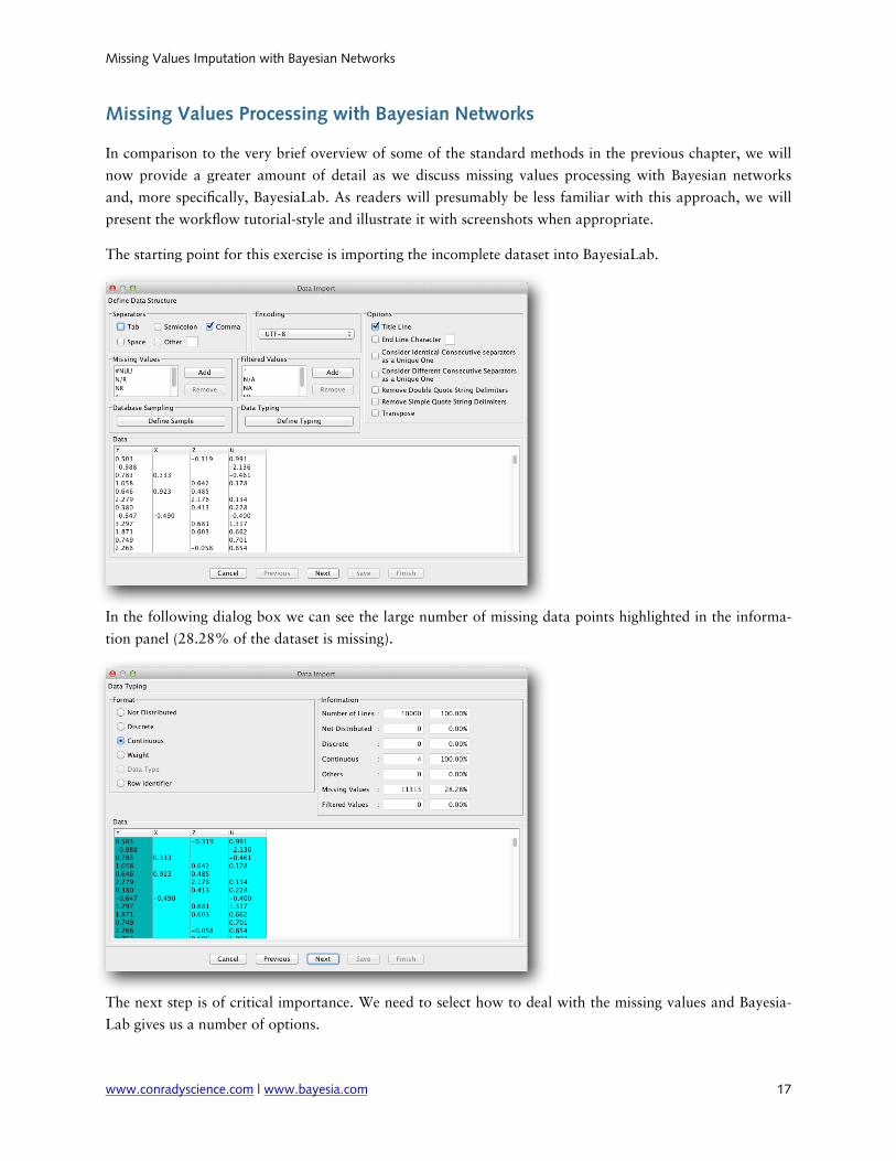
The starting point for this exercise is importing the incomplete dataset into BayesiaLab.

In the following dialog box we can see the large number of missing data points highlighted in the informa-tion panel (28.28% of the dataset is missing).

The next step is of critical importance. We need to select how to deal with the missing values and Bayesia-Lab gives us a number of options.







The first option, Filter, allows us to perform listwise/casewise deletion, which, as before, is not feasible as no data points would remain available for analysis. The second option, Replace By, refers to mean imputa-tion5, which, with all its drawbacks, can be applied here within the Bayesian network framework. We men-tion means imputation for the sake of completeness, rather than as a recommendation. Also, Filter and/or Replace By can be selectively applied on a variable-by-variable basis. Once one of these static missing value processing options is applied to the selected variables, BayesiaLab considers these variables as completely observed. In other words, this approach would purely be a pre-treatment generating fixed values.

For our example we shall instead choose from among the BayesiaLab-specific options, i.e. Static Comple-tion, Dynamic Completion and Structural EM, which will subsequently explain:

Static Completion

Static Completion resembles mean imputation, but differs in one important aspect: while mean imputation is deterministic, Static Completion performs random draws from the marginal distributions of the observed data points and saves these randomly drawn values as “placeholder values,” at the completion of the import process. Our artificially-created missing values are thus being filled in instantly with estimated values, which would then permit a parameter estimation as in the case of a complete data set. BayesiaLab highlights the variables that contain missing values with a small question mark icon.



5 Mean imputation applies to continuous and discrete numerical variables. For categorical variables the modal values

are imputed.





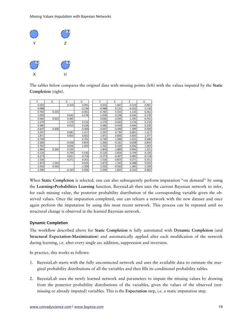
The tables below compares the original data with missing points (left) with the values imputed by the Static Completion (right).

Y X Z U0.503 )0.319 0.991)0.988 )2.1360.783 0.333 )0.4611.058 0.642 0.1780.646 0.923 0.4852.279 2.176 0.1340.380 0.413 0.228)0.647 )0.490 )0.4003.297 0.681 1.3171.871 0.603 0.6620.749 0.7012.266 )0.058 0.8542.762 0.696 1.0031.804 0.264 0.3200.110 0.749 0.130)0.273 0.851 )0.7181.526 0.271 0.351)1.873 )1.342 0.024)1.932 )0.563 )1.2092.206 )0.163 0.506

Y X Z U0.503 1.967 -0.319 0.991-0.988 0.131 -0.162 -2.1360.783 0.333 1.133 -0.4611.058 0.238 0.344 0.1780.646 -2.035 1.195 -0.7612.279 -0.693 2.176 0.1340.380 -0.920 0.640 0.228-0.647 -0.490 1.589 -0.4003.297 0.739 0.681 1.3171.871 0.606 0.603 1.3770.749 1.068 -1.021 0.5882.266 -0.161 -0.058 0.8542.762 0.329 0.696 1.0031.804 -1.880 0.969 1.2210.110 -2.826 0.749 0.130-0.273 -0.407 0.485 -0.7181.526 0.853 0.271 0.351-1.873 -1.342 -0.488 0.024-1.932 -0.563 1.383 -1.2092.206 1.863 -0.163 -0.862

When Static Completion is selected, one can also subsequently perform imputation “on demand” by using the Learning>Probabilities Learning function. BayesiaLab then uses the current Bayesian network to infer, for each missing value, the posterior probability distribution of the corresponding variable given the ob-served values. Once the imputation completed, one can relearn a network with the new dataset and once again perform the imputation by using this most recent network. This process can be repeated until no structural change is observed in the learned Bayesian network.

Dynamic Completion

The workflow described above for Static Completion is fully automated with Dynamic Completion (and Structural Expectation-Maximization) and automatically applied after each modification of the network during learning, i.e. after every single arc addition, suppression and inversion.

In practice, this works as follows:

1. BayesiaLab starts with the fully unconnected network and uses the available data to estimate the mar-ginal probability distributions of all the variables and then fills its conditional probability tables.

2. BayesiaLab uses the newly learned network and parameters to impute the missing values by drawing from the posterior probability distributions of the variables, given the values of the observed (not-missing or already imputed) variables. This is the Expectation step, i.e. a static imputation step.







3. BayesiaLab uses this new dataset, which no longer contains missing values, to learn the structure and estimate the corresponding parameters. This is the Maximization step.

4. The process alternates the Expectation and Maximization steps until convergence is achieved.

In this process the Bayesian network will grow from an initially unconnected network and evolve in its structure until its final state is reached.

Depending on the number of variables, the chosen learning algorithm and the network complexity6, hun-dreds or thousands of iterations may be calculated. The final imputed dataset then remains available for subsequent analysis or export.

In the context of this iterative learning process, and beyond merely estimating the missing values, we have also established an interpretable structure of the underlying domain in the form of a Bayesian network. From a qualitative perspective, this network does indeed reflect all the relationships that we originally cre-ated with the DGP formula and the covariance structure form the original sampling process.

Having this fully estimated network available, we can also retrieve the quantitative knowledge contained therein and obtain the “parameters” of the structure. We are using parameters here loosely (hence the quo-tation marks), as the Bayesian network structures in BayesiaLab are always entirely nonparametric.

To obtain these quantitative characteristics from the network, we can immediately perform the Target Mean Analysis (Direct Effects), which produces a plot of the interactions of U, Z and X with Y.7 Even though there is no assumption of linearity in BayesiaLab, the shape of the curve confirms than the learned network indeed approximates the linear function from the DGP formula.



6 In BayesiaLab, the network complexity can be managed with the Structural Coefficient.

7 Our white paper, Direct Effects and Causal Inference, describes details of the Direct Effects computation.





Computing the Direct Effect on Target provides us with the partial derivative of each of the above curves

∂y∂x, ∂y∂z, ∂y∂u

⎛⎝⎜

⎞⎠⎟

at the mean value of each variable:

Direct Effects on Target YStandardizedDirect,Effect

U 0.4283 1.0311Z 0.3733 1.0238X 0.3514 0.9733

Node Direct,Effect

The derivates represent the slopes of each curve (at the mean of each of the independent variables), and now assuming linearity, we can directly interpret the Direct Effects as the parameter estimates of our DGP function:8

βx = 1.031βz = 1.024βu = 0.973

These values are indeed very close to the true parameters. Even though we are giving these results a linear interpretation, it is important to point out that a functional form was neither assumed in the missing data estimation process, nor in the Bayesian network structural and parametric learning.



8 We can do this here as we have no intercept in the DGP function.





Alternatively, we can also save the estimated missing values for subsequent external analysis with classical methods (Data>Imputation).

This will prompt a choice of imputation method, which is very important.

We can maintain the “uncertainty” of the missing data by selecting the option, “Choose the Values Accord-ing to the Law.” This means that each to-be-saved value will be drawn from the conditional probability distribution of each variable. This option is clearly not the optimal choice at the individual level (one has to choose the Maximum Probability for that purpose), but it allows retaining the variance, i.e. the uncertainty of the original data.

With this fully imputed dataset, and assuming linearity for the DGP, we can once again use traditional methods, e.g. OLS, to compute the parameter estimates. In this case, we would obtain the following:

βx = 0.954 (0.013)βz = 0.898 (0.013)βu = 1.163 (0.012)Constant = 0.026

Given that no functional form was utilized in the missing values imputation process, and given the variables were discretized, the results are extremely useful.







Nonlinear Example

As the previous (linear) example turned out to be manageable with a number of different approaches, we will now look at a more challenging situation. It is challenging because we introduce nonlinear relationships between variables.

Data Generating Process (DGP)

As before, the synthetic dataset consists of 10,000 observations of a row vector, A=[X,Z,U], which follows a multivariate normal distribution:

A N3(µ,Σ)

µ =000

⎛

⎝

⎜⎜

⎞

⎠

⎟⎟

Σ =1 0.5 0.50.5 1 0.50.5 0.5 1

⎛

⎝

⎜⎜

⎞

⎠

⎟⎟

So, we use the same DGP as for the linear example, but now create a new function for Y that combines ex-ponential, quadratic and linear terms:

yi = exi+ zi

2 + ui , i ∈[1...n], n = 10,000

Our complete set of observations is thus contained in this matrix:

ex1+ z12 + u1 x1 z1 u1

exn+ zn2 + un xn zn un

⎛

⎝

⎜⎜⎜

⎞

⎠

⎟⎟⎟

With our knowledge of the underlying DGP, we can describe the functional form as:

y = βxex + βzz

2 + βuu , with the known parameters βx = βz = βu = 1 .

In our subsequent analysis we will treat these parameters as unknown and compute estimates for them from the manipulated dataset, i.e. once it is subjected to the Missing Data Mechanism.

The following plot illustrates the shape and the distribution of the individual terms, i.e. Y as a function of X, Z and U.







Bayesian Network Representation

As shown in the linear case, Bayesian networks can provide an intuitive representation of a domain with missing values and quasi automatically provide missing value estimates. While this is certainly convenient, it is not necessarily a “unique selling point” for Bayesian networks. The situation is quite different when mov-ing to nonlinear domains. A number of statistical software packages do allow performing advanced meth-ods, such as multiple imputation, even in nonlinear domains. However, the process of specifying an imputa-tion model in the nonlinear case is a scientific modeling effort on its own and few non-statisticians dare ven-ture into this specialized field (van Buuren, 2007).

We believe that the “integral” missing values processing in BayesiaLab provides a critical advantage to the applied researcher, who might otherwise not even attempt to formally deal with missing values in nonlinear models.

However, before we move on to missing values processing, we will first establish that the original variables’ nonlinear dynamics can indeed be captured in a Bayesian network learned with BayesiaLab. While Bayesia-Lab cannot discover the functional form of the DGP formula per se, it can learn the relationships on a non-parametric basis.

We will omit the data import steps, as they are analogous to the process shown before, and rather fast-forward to the presentation of the final network:







We can see that the overall network structure reflects the relationships that were stipulated by both the co-variance matrix and the DGP formula. More specifically, we can check the Pearson’s correlation coefficients of the linear relationships between X, Z and U, by displaying the values on the relevant arcs (Analy-sis>Graphic>Pearson’s Correlation).







The computed values are indeed close to the 0.5 stated in the covariance matrix.9 It is important to point out here again that BayesiaLab does not compute the correlation on the assumption of a linear function, as BayesiaLab is entirely nonparametric.

We now turn to the nonlinear relationships specified in the DGP formula. To see how the principal dynam-ics with Y are reflected in the Bayesian network, we illustrate the dependencies in the following plot of the Target Mean Analysis by Direct Effect:

We can visually identify the exponential, quadratic and linear shape of the curves and thus judge that the complete dataset is adequately represented.

Missing Data Mechanism

Now that we have a framework for the complete dataset (with all its mutual dependencies) in place, we can start deleting observations. The MDM is very similar to the one applied earlier, with the only change being in the parameters of the logistic function, which now generate a “softer” application of the value deletion (see graph).



9 Given that the standard deviation was set to 1, the covariance equals the correlation coefficient.





P(xi = missing) = 1− 1

1+ eyi3

,

P(zi = missing) = 1− 1

1+ e−yi3

,

P(ui = missing) = 0 if xi=missing and yi=missingelse 1

⎧⎨⎪

⎩⎪

⎫⎬⎪

⎭⎪

-10 -5 5 10y

0.2

0.4

0.6

0.8

PHmissingL

Upon application of the MDM, we once again have the issue that not a single observation is complete.

With that, we have a threefold challenge:

1. Data missing at random

2. No complete set of observations

3. Unknown dependencies between all variables, both for DGP and MDM.

To further illustrate this challenge, we plot the remaining data points post-MDM. Given that we know the original DGP, we can just about make out the functional form, although the exponential and the linear term seem to “blur” together.







Another way to represent the MDM is by plotting Y vs. X (red, complete) and Y vs. X (black, missing), shown below:

From a traditional statistical perspective, it would indeed present a formidable challenge to identify the functional form, its parameters and then impute the missing values.

Bayesian Network Learning & Missing Values Imputation

Within the Bayesian network framework this is much simpler, as all three problems can be dealt within a single process, i.e. Unsupervised Learning with Dynamic Completion of missing values.

Unsupervised Learning

As described in the linear case, BayesiaLab iteratively alternates learning and imputation until convergence is achieved. The graphs below represent a selection of steps from the learning process.







As there is no functional form recorded in BayesiaLab, we need to look at a plot of the probabilistic de-pendencies to see whether we have successfully recovered the underlying dynamics. More specifically, we need to use Target Mean Analysis by Direct Effects to decompose the overall function (now represented by the Bayesian network) into the individual components that reflect the DGP terms.

A first visual inspection suggests that BayesiaLab has indeed captured the salient points of the DGP (keeping in mind that the variables have been discretized). As BayesiaLab is entirely nonparametric, we cannot re-trieve parameter estimates, rather we can utilize the learned functions as they are encoded with the structure of the Bayesian network and the associated conditional probability tables.

However, computing the Direct Effect on Target provides us with the partial derivative of each of the above

Direct Effect Function curves ∂y∂x, ∂y∂z, ∂y∂u

⎛⎝⎜

⎞⎠⎟

at the estimated mean value of each variable.







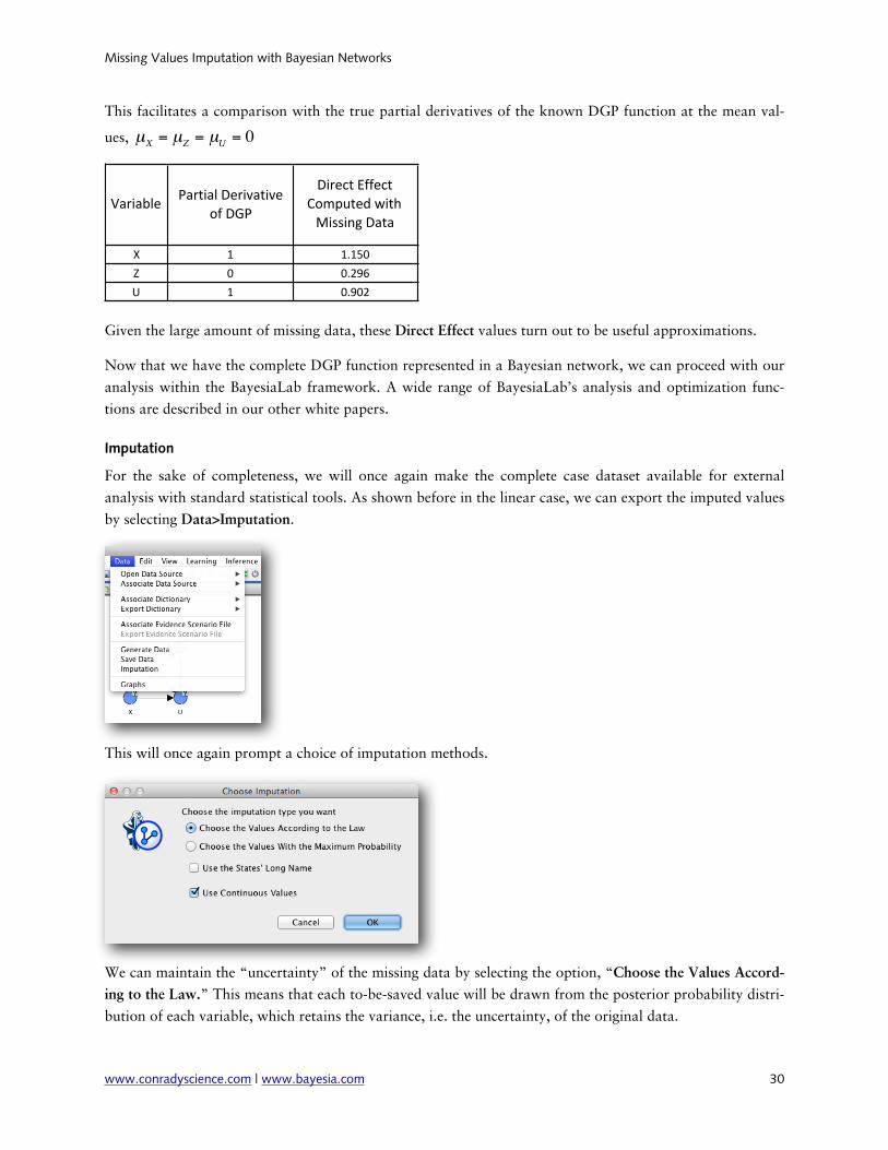
This facilitates a comparison with the true partial derivatives of the known DGP function at the mean val-

ues, µX = µZ = µU = 0

Variable Partial*Derivative*of*DGP

Direct*Effect*Computed*with*Missing*Data

X 1 1.150Z 0 0.296U 1 0.902

Given the large amount of missing data, these Direct Effect values turn out to be useful approximations.

Now that we have the complete DGP function represented in a Bayesian network, we can proceed with our analysis within the BayesiaLab framework. A wide range of BayesiaLab’s analysis and optimization func-tions are described in our other white papers.

Imputation

For the sake of completeness, we will once again make the complete case dataset available for external analysis with standard statistical tools. As shown before in the linear case, we can export the imputed values by selecting Data>Imputation.

This will once again prompt a choice of imputation methods.

We can maintain the “uncertainty” of the missing data by selecting the option, “Choose the Values Accord-ing to the Law.” This means that each to-be-saved value will be drawn from the posterior probability distri-bution of each variable, which retains the variance, i.e. the uncertainty, of the original data.







The complete dataset is now saved as a CSV file and can be accessed by any statistical program for further analysis. Assuming that we know the functional form of the DGP (or are able to guess it from the plot of the Target Mean Analysis seen earlier), we can then use the filled-in dataset to estimate the parameters. For instance, we can use OLS to compute the parameter estimates for the functional form of the DGP:

y = βxex + βzz

2 + βuu

In this case, we would obtain the following coefficients, which are once again very close to the true values of the parameters:

βx = 1.025 (0.013)βz = 0.998 (0.013)βu = 1.153 (0.020)

Summary Nonlinear Example

Despite the large number of missing values, BayesiaLab’s learning and imputation algorithms allowed us to discover the DGP and simultaneously estimate the missing values. As a result, we now have a fully inte-grated process that does no longer require a separate treatment of the DGP and the MDM thus facilitating an accelerated modeling workflow for researchers and analysts.

Summary & Outlook

The proposed integrated approach to missing values processing and imputation is certainly a practical bene-fit to the applied researcher, especially given Burton and Altman’s serious concerns stated in the introduc-tion. While missing data has been the proverbial “elephant in the room”, there is now even less of an excuse for not squarely addressing the problem.

Beyond merely addressing a flaw in data, our new approach may actually lend itself to broader applications. With this tool in hand, we may see an opportunity to rephrase other kinds of problems and treat them as missing values problems. One could think of state space models, multiple sensor fusion or mixed-frequency models in this context. However, these extensions go beyond the scope of this paper will need to be covered in future work.







Appendix

About the Authors

Stefan Conrady

Stefan Conrady is the cofounder and managing partner of Conrady Applied Science, LLC, a privately held consulting firm specializing in knowledge discovery and probabilistic reasoning with Bayesian networks. In 2010, Conrady Applied Science was appointed the authorized sales and consulting partner of Bayesia S.A.S. for North America.

Stefan Conrady studied Electrical Engineering in Germany and has extensive management experience in the fields of product planning, marketing and analytics, working at Daimler and BMW Group in Europe, North America and Asia. Prior to establishing his own firm, he was heading the Analytics & Forecasting group at Nissan North America.

Lionel Jouffe

Dr. Lionel Jouffe is cofounder and CEO of France-based Bayesia S.A.S. Lionel Jouffe holds a Ph.D. in Com-puter Science and has been working in the field of Artificial Intelligence since the early 1990s. He and his team have been developing BayesiaLab since 1999 and it has emerged as the leading software package for knowledge discovery, data mining and knowledge modeling using Bayesian networks. BayesiaLab enjoys broad acceptance in academic communities as well as in business and industry. The relevance of Bayesian networks, especially in the context of consumer research, is highlighted by Bayesia’s strategic partnership with Procter & Gamble, who has deployed BayesiaLab globally since 2007.







References

Allison, P.D. “Multiple imputation for missing data: A cautionary tale.” Sociological methods and Research 28, no. 3 (2000): 301–309.

Allison, Paul D. Missing Data. 1st ed. Sage Publications, Inc, 2001.

Barber, David. Bayesian Reasoning and Machine Learning. Cambridge University Press, 2011.

“BBN_Introduction_V13.pdf”, n.d.

Burton, A, and D G Altman. “Missing covariate data within cancer prognostic studies: a review of current reporting and proposed guidelines.” British Journal of Cancer 91 (June 8, 2004): 4-8.

Van Buuren, S. “Multiple imputation of discrete and continuous data by fully conditional specification.” Statistical Methods in Medical Research 16, no. 3 (2007): 219.

Conrady, Stefan, and Lionel Jouffe. “Introduction to Bayesian Networks - Practical and Technical Perspec-tives”. Conrady Applied Science, LLC, February 15, 2011. http://www.conradyscience.com/index.php/introduction-to-bayesian-networks.

Copas, John B., and Guobing Lu. “Missing at random, likelihood ignorability and model completeness.” The Annals of Statistics 32 (April 2004): 754-765.

“Data Imputation for Missing Values: Statnotes, from North Carolina State University, Public Administra-tion Program”, n.d. http://faculty.chass.ncsu.edu/garson/PA765/missing.htm.

Dempster, A. P., N. M. Laird, and D. B. Rubin. “Maximum Likelihood from Incomplete Data via the EM Algorithm.” Journal of the Royal Statistical Society. Series B (Methodological) 39, no. 1 (January 1, 1977): 1-38.

Enders, Craig K. Applied Missing Data Analysis. 1st ed. The Guilford Press, 2010.

Heckerman, D. “A tutorial on learning with Bayesian networks.” Innovations in Bayesian Networks (2008): 33–82.

Heitjan, Daniel F., and Srabashi Basu. “Distinguishing ‘Missing at Random’ and ‘Missing Completely at Random’.” The American Statistician 50 (August 1996): 207.

“Historical Stock Data”, n.d. http://pages.swcp.com/stocks/.

Horton, N.J., and S.R. Lipsitz. “Multiple Imputation in Practice.” The American Statistician 55, no. 3 (2001): 244–254.

Howell, David C. “Treatment of Missing Data”, n.d. http://www.uvm.edu/~dhowell/StatPages/More_Stuff/Missing_Data/Missing.html.

Lin, J.H., and P.J. Haug. “Exploiting missing clinical data in Bayesian network modeling for predicting medical problems.” Journal of biomedical informatics 41, no. 1 (2008): 1–14.

Little, Roderick J. A., and Donald B. Rubin. Statistical Analysis with Missing Data, Second Edition. 2nd ed. Wiley-Interscience, 2002.

“Missing completely at random - Wikipedia, the free encyclopedia”, n.d. http://en.wikipedia.org/wiki/Missing_completely_at_random.

de Morais, S.R., and A. Aussem. “Exploiting Data Missingness in Bayesian Network Modeling.” In Ad-vances in Intelligent Data Analysis VIII: 8th International Symposium on Intelligent Data Analysis, IDA 2009, Lyon, France, August 31-September 2, 2009, Proceedings, 5772:35, 2009.

“NCES Statistical Standards, Appendix B, Evaluating the Impact of Imputations for Item Non-Response”, n.d. http://nces.ed.gov/statprog/2002/appendixb3.asp.



http://www.conradyscience.com/index.php/introduction-to-bayesian-networks

http://www.conradyscience.com/index.php/introduction-to-bayesian-networks

http://faculty.chass.ncsu.edu/garson/PA765/missing.htm

http://faculty.chass.ncsu.edu/garson/PA765/missing.htm

http://pages.swcp.com/stocks/

http://pages.swcp.com/stocks/

http://www.uvm.edu/~dhowell/StatPages/More_Stuff/Missing_Data/Missing.html

http://www.uvm.edu/~dhowell/StatPages/More_Stuff/Missing_Data/Missing.html

http://en.wikipedia.org/wiki/Missing_completely_at_random

http://en.wikipedia.org/wiki/Missing_completely_at_random

http://nces.ed.gov/statprog/2002/appendixb3.asp

http://nces.ed.gov/statprog/2002/appendixb3.asp





Riphahn, Regina T., and Oliver Serfling. “Item non-response on income and wealth questions.” Empirical Economics 30 (September 2005): 521-538.

Rubin, Donald B. “Inference and missing data.” Biometrika 63, no. 3 (December 1, 1976): 581 -592.

———. Multiple Imputation for Nonresponse in Surveys. Wiley-Interscience, 2004.

Schafer, J.L. Analysis of Incomplete Multivariate Data. 1st ed. Chapman and Hall/CRC, 1997.

Schafer, J.L., and M.K. Olsen. “Multiple imputation for multivariate missing-data problems: A data ana-lyst’s perspective.” Multivariate Behavioral Research 33, no. 4 (1998): 545–571.

“SOLAS Missing Data Analysis | Multiple Imputation | Missing Data Analysis Software @ Solas for Missing Data Analysis”, n.d. http://www.solasmissingdata.com/.

“SPSS Missing Values 17.0 User’s Guide”. SPSS Inc., n.d.

Wayman, J.C. “Multiple imputation for missing data: What is it and how can I use it.” In Annual Meeting of the American Educational Research Association, 1–16, 2003.

“www.missingdata.org.uk”, n.d. http://missingdata.lshtm.ac.uk/.



http://www.solasmissingdata.com

http://www.solasmissingdata.com

http://www.missingdata.org.uk

http://www.missingdata.org.uk

http://missingdata.lshtm.ac.uk

http://missingdata.lshtm.ac.uk





Contact Information

Conrady Applied Science, LLC

312 Hamlet’s End WayFranklin, TN 37067USA+1 888-386-8383 [email protected]

Bayesia S.A.S.

6, rue Léonard de VinciBP 11953001 Laval CedexFrance+33(0)2 43 49 75 [email protected]

Copyright

© 2011 Conrady Applied Science, LLC and Bayesia S.A.S. All rights reserved.

Any redistribution or reproduction of part or all of the contents in any form is prohibited other than the following:

• You may print or download this document for your personal and noncommercial use only.

• You may copy the content to individual third parties for their personal use, but only if you acknowledge Conrady Applied Science, LLC and Bayesia S.A.S. as the source of the material.

• You may not, except with our express written permission, distribute or commercially exploit the content. Nor may you transmit it or store it in any other website or other form of electronic retrieval system.















VVImp Missing Values v14

Documents

Transcript of VVImp Missing Values v14