
VSC-HVDC System Modeling and · PDF fileVSC-HVDC System Modeling and Validation ROBERT...
132
VSC-HVDC System Modeling and Validation ROBERT ROGERSTEN Master’s Degree Project Stockholm, Sweden 2014 XR-EE-EPS 2014:003
Transcript of VSC-HVDC System Modeling and · PDF fileVSC-HVDC System Modeling and Validation ROBERT...

VSC-HVDC System Modeling andValidation
ROBERT ROGERSTEN
Master’s Degree ProjectStockholm, Sweden 2014
XR-EE-EPS 2014:003

Abstract
The performance of traditionally used converter control strategies dependson the ac system conditions. Particularly, the ac system strength is a limitingfactor for converter controls to perform well. This work is motivated bythe rapid proliferation of high-voltage dc technology, which enables differentcontrol structures to be simulated using different simulation tools. The firstpart of this thesis investigates a generic converter control model on differentsimulation platforms and implementations. The second part exploits theabove-mentioned limiting factor for converter controls to perform well.
In this thesis, a control implementation is tailored to replicate the be-havior of another control implementation on different software. In orderto ensure that software implementations not become alienated from reality,comparisons to a manufacturer’s black-box are also carried out. Furthermore,this thesis demonstrates how many converter stations are linked together bya dc transmission network. A previously proposed control method, power-synchronization control, has been demonstrated to perform well on a point-to-point high-voltage direct current link in connection to a weak ac system.In this thesis, the potential of power-synchronization control is demonstratedin a multi-terminal dc grid with one very weak ac system connection.

Acknowledgments
I would like to thank Dr. Luigi Vanfretti and PhD student Wei Li formaking this project possible. I also wish to thank Dr. Lidong Zhang andDr. Pinaki Mitra for their helpful support during this project.

Contents
1 Introduction 41.1 Background and Motivation . . . . . . . . . . . . . . . . . . . 4
1.1.1 Control Models on Different Simulation Platforms . . 51.1.2 Controller Performance Comparison . . . . . . . . . . 51.1.3 Power-Synchronization Control . . . . . . . . . . . . . 5
1.2 Problem Definition and Objectives . . . . . . . . . . . . . . . 61.3 Limitations . . . . . . . . . . . . . . . . . . . . . . . . . . . . 71.4 General Overview . . . . . . . . . . . . . . . . . . . . . . . . . 7
2 High-Voltage Direct-Current Transmission and Control 92.1 Conversion Methods . . . . . . . . . . . . . . . . . . . . . . . 9
2.1.1 Voltage Source Converter Systems . . . . . . . . . . . 92.1.2 Classical HVDC Systems . . . . . . . . . . . . . . . . 10
2.2 Modeling of Voltage Source Converters . . . . . . . . . . . . . 102.3 VSC-HVDC Transmission . . . . . . . . . . . . . . . . . . . . 11
2.3.1 Point-to-Point VSC-HVDC Systems . . . . . . . . . . 122.3.2 Multi-Terminal VSC-HVDC Systems . . . . . . . . . . 12
2.4 Control Methods for VSC-HVDC Systems . . . . . . . . . . . 132.4.1 Vector-Current Control . . . . . . . . . . . . . . . . . 132.4.2 Power-Synchronization Control . . . . . . . . . . . . . 172.4.3 Droop Control . . . . . . . . . . . . . . . . . . . . . . 19
3 Implementation and Design in PSCAD 223.1 Implementation Approach . . . . . . . . . . . . . . . . . . . . 223.2 PSCAD Terminology . . . . . . . . . . . . . . . . . . . . . . . 233.3 Graphical Implementation in PSCAD . . . . . . . . . . . . . 24
3.3.1 The Average Value Model . . . . . . . . . . . . . . . . 243.3.2 The Control Module . . . . . . . . . . . . . . . . . . . 263.3.3 Multi-Terminal VSC-HVDC System in PSCAD . . . . 32
3.4 Control Implementation in PSCAD using Code Generation . 343.4.1 Simulink C Code Generation . . . . . . . . . . . . . . 343.4.2 Fortran Integration with C code . . . . . . . . . . . . 363.4.3 Linking a library to PSCAD . . . . . . . . . . . . . . . 38

CONTENTS 2
3.4.4 Overall Integration for the Code Implementation . . . 403.4.5 Scalability of the Proposed Implementation . . . . . . 44
4 Controller Performance Comparisons and Analysis 464.1 Methodology . . . . . . . . . . . . . . . . . . . . . . . . . . . 47
4.1.1 Numerical Comparisons . . . . . . . . . . . . . . . . . 474.1.2 Fault Impedance and System Configuration . . . . . . 48
4.2 Controller Performance Comparisons . . . . . . . . . . . . . . 484.3 Controller Performance Analysis and Results . . . . . . . . . 514.4 Black-Box Model Comparisons . . . . . . . . . . . . . . . . . 52
5 Power-Synchronization Control Analysis 555.0.1 The DC Grid Test System . . . . . . . . . . . . . . . . 55
5.1 Interconnection of a Weak AC System . . . . . . . . . . . . . 585.1.1 Estimation of the Short-Circuit Ratio . . . . . . . . . 585.1.2 Step Response of the Active-Power Controller . . . . . 585.1.3 Three-Phase Fault at the Bus of Converter A . . . . . 59
6 Conclusions and Further Work 636.1 Model Design and Controller Comparisons . . . . . . . . . . . 63
6.1.1 Graphical Implementation . . . . . . . . . . . . . . . . 636.1.2 Code Implementation . . . . . . . . . . . . . . . . . . 646.1.3 Further Work . . . . . . . . . . . . . . . . . . . . . . . 646.1.4 Black-Box Model Comparison . . . . . . . . . . . . . . 65
6.2 Power-Synchronization Control . . . . . . . . . . . . . . . . . 65
7 Bibliography 66
A Voltage Plots During Faults 69
B Graphical Implementation 73B.1 Step of the Active- and Reactive-Power Controller . . . . . . 73B.2 Three-Phase Faults (Fault Scenarios 3 to 5) . . . . . . . . . . 78B.3 Single-Phase Faults (Fault Scenarios 6 to 8) . . . . . . . . . . 85
C Code Implementation 92C.1 Step of the Active- and Reactive-Power Controller . . . . . . 92C.2 Three-Phase Faults (Fault Scenarios 3 to 5) . . . . . . . . . . 97C.3 Single-Phase Faults (Fault Scenarios 6 to 8) . . . . . . . . . . 104
D Black-Box Model Comparisons 111D.1 Step of the Active- and Reactive-Power Controller . . . . . . 111D.2 Three-Phase Faults at Rectifier Side (Fault Scenarios 3 to 5) 114D.3 Single-Phase Faults at Rectifier Side (Fault Scenarios 6 to 8) 118D.4 Three-Phase Faults at Inverter Side (Fault Scenarios 3 to 5) . 122

CONTENTS 3
D.5 Single-Phase Faults at Inverter Side (Fault Scenarios 6 to 8) . 126

Chapter 1
Introduction
The revival of direct current (dc) for long-distance power transmission beganin 1954 when ASEA, a predecessor of ABB, linked the island of Gotland tomainland Sweden with high-voltage direct-current (HVDC) lines. However,the history of dc began before that. Thomas Edison lost the war of dc againstalternating current (ac) and in the 1890s it became clear that ac was moreefficient at transmitting electricity over long distances. However, dc hasstaged a roaring comeback during recent years because of several reasons.One reason is the increase in electricity consumption throughout the world.In Europe alone, total electricity consumption has increased by 32.8% from1990 to 2007. As a result, the European high-voltage alternating-current(HVAC) grid is operating very close to its limits.
Today, there are many HVDC projects in operation worldwide. Powertransmission using dc allows for transporting large amounts of electricityacross long distances, exceeding the transport capacity of ac lines. ClassicalHVDC technology utilizes thyristors for power conversion. However, recently,a new more advantageous HVDC technology based on voltage source con-verters (VSC) has emerged [1, 2]. The VSC technology utilizes gate-turn-offthyristors (GTOs) or in most industrial cases insulated gate bipolar transis-tors (IGBTs) for switching. For example can VSC-HVDC systems addressissues regarding power transmission, asynchronous network interconnections,and stability support.
1.1 Background and Motivation
In this section, the background and motivation of the project are discussed.Simulation results from generic control models often differ between simulationplatforms. Therefore, part of this work is motivated by the need to investigatesuch differences and to facilitate the transfer between simulation platforms.Another motivation for this project is the increasing need to compare controlmodels for VSC-HVDC systems used in academic research to control models

1.1. BACKGROUND AND MOTIVATION 5
from industry.This thesis will discuss the commonly used control method referred to
as vector-current control. It will also discuss the alternative control methodreferred to as power-synchronization control. Power-synchronization controlhas been implemented on control models for comparison to the traditionallyused vector-current control.
1.1.1 Control Models on Different Simulation Platforms
In this thesis, a generic control model is developed based on the Cigre genericcontrol model. Cigre is a working group that deals with HVDC transmissionand power electronics for use in transmission and distribution networks. TheCigre working group has developed a generic control model in Simulink, whichwill be used as a reference model in this work. This thesis investigate thegeneric control model on different simulation platforms and implementations.Therefore, the control model has been developed in PSCAD1. Furthermore,the C code has been extracted from the Simulink model for implementationin PSCAD2. Using this approach, the controls in PSCAD can be tailored toreplicate the behavior of Simulink very well.
1.1.2 Controller Performance Comparison
As already discussed, the dc grid developments and applications have maderapid progress during recent years. Among with the technology advancesthere exist many commercial and trade secret reasons from industry regardingVSC-HVDC converter stations. Particularly, there are plentiful questionsregarding the control of VSC-HVDC converters. There is also a crucialneed of realistic data regarding controller performance. Without consistentcomparison and validation with the realistic data used in industry, theacademic research could become alienated from reality. This motivates thecomparison between generic control models and realistic results from industrycarried out in this thesis.
1.1.3 Power-Synchronization Control
The theory of power-synchronization control is detailed in [3]. The potentialof power-synchronization is revealed when the VSC is connected to a weakac system. As discussed in [4], a description of the strength of the ac system
1In the past two sentences both PSCAD and Simulink (an extension of Matlab) hasbeen mentioned. PSCAD and Simulink are graphical tools that can be used for simulationof electric power systems, for more information see chapter 3
2To distinguish between these implementations, the traditional way to build a modelwill be referred to as the graphical implementation, while the other approach will bereferred to as the C code implementation.

1.2. PROBLEM DEFINITION AND OBJECTIVES 6
relative to the power rating of the HVDC link can be given by the short-circuit ratio (SCR). Thus, if the calculated SCR is low the ac system is weak.It is discussed in [3] that the conventional thyristor based HVDC systemcannot work properly if the SCR is low.
In contrast to the conventional thyristor based HVDC system, the VSC-HVDC system can produce its own voltage waveform independent of theac system, which means that a VSC-HVDC system has the potential to beconnected to very weak ac systems. However, with the traditional vector-current control the potential of the VSC is not fully utilized [3, 5, 6, 7]. Vector-current control inherits poor performance for weak ac system connections.
Motivated by this fact, power-synchronization control is implementedas an alternative control method for comparison of control performance ona system with very low SCR. Thus far, power-synchronization control hasonly been applied to point-to-point interconnections [6]. Therefore, power-synchronization control is implemented in a multi-terminal VSC-HVDCsystem in this thesis. This work is also presented in [8].
1.2 Problem Definition and Objectives
In this thesis, a control model for VSC-HVDC systems is implemented inPSCAD based on the Cigre generic control model developed in Simulink.The Simulink model will be considered as a reference for the generic controlmodel. Therefore, comparisons to the Simulink model are performed inorder to ensure that deviations are not too large. Further, comparisonsare performed with a manufacturer’s black-box model. These comparisonstogether with an analysis of how power-synchronization control behaves in amulti-terminal dc system will form this thesis. Basically, the objectives willbe:
1) Compare and analyze the two control methods, vector-current control,and power-synchronization control in a multi-terminal dc system.
2) Compare the graphical implementation and the C code implementationto the Simulink model.
3) Compare the best of these implementations to the manufacturer’sblack-box model3.
Working against these objectives led to two chapters that presents theresults: (i) controller performance comparisons and analysis, and (ii) power-synchronization control analysis. Figure 1.1 illustrates this by a flowchart.The grey box in the bottom left of figure 1.1 represents how objective 1)is accomplished, while the grey box in the bottom right represents howobjective 3) is accomplished. The two grey boxes in the middle corresponds
3The best here will be the C code implementation, it will be explained later that thisimplementation has almost a perfect match to the Simulink model.

1.3. LIMITATIONS 7
Simulink implementation
Code implementation
PSCAD
Manufacturer’s black-box model
Comparisons of code
implementation
Analysis and comparisons in a multi-terminal dc
system
Comparisons of graphical
implementation
PSCAD
implementation
Power-
synchronization control
implementation
Comparisons of black-box model
Reference model
Power-Synchronization Control Analysis
Controller Performance Comparisons and Analysis
Figure 1.1: Flowchart of different model implementations, which led to the main resultsin this thesis. The grey box in the bottom left yields the chapter calledpower-synchronization control analysis. The other three grey boxes comparedifferent implementations according to the flow chart. These comparisonswill yield the chapter called controller performance comparisons and analysis.
to objective 2). Note that the grey boxes leads to the two final chapterspresented in this thesis.
1.3 Limitations
This project will focus on the VSC-HVDC systems and the control methodsused for such systems. The controls of a VSC-HVDC system can be dividedinto lower level controls and upper level controls. The upper level controlsystem calculates three phase voltage references and feeds them into the lowerlevel control system. The lower level control system will not be discussed inthis thesis. Thus, the emphasis will be on upper level control of VSC-HVDCsystems.
1.4 General Overview
This thesis will be structured as follows. Chapter 2 introduces HVDCtransmission and the control strategies used for VSC-HVDC systems. Firstthe traditional HVDC technology and the VSC technology are discussed.The point-to-point model and the HVDC grid are introduced. Further, thecontrol strategies used in this thesis are discussed.
Chapter 3 explains how the model has been developed and implemented

1.4. GENERAL OVERVIEW 8
in PSCAD. Chapter 3 also discusses general terminology used when workingin PSCAD. This terminology is useful when discussing different type ofobjects implemented in PSCAD. The generic control model is constructed intwo ways, graphically and by the use of C code. The first part of chapter 3explains how to construct the model graphically, while the last part showshow to construct the model using C code extracted from the Simulink model.
Chapter 4 demonstrates the performance of vector-current control indetail. Several comparisons are carried out between software implementations.Also, comparisons with a manufacturer’s black-box model are carried out.
Chapter 5 will discuss the results from simulations using power-synchronizationcontrol. Particularly, these simulations are carried out in a multi-terminalVSC-HVDC system.
Finally, chapter 6 draws some conclusions and discusses further work.

Chapter 2
High-Voltage Direct-CurrentTransmission and Control
A variety of technical, economical and environmental reasons are forcing thetraditionally ac power transmission development to rethink. An importantfactor is the need of increased power carrying capability of transmission lines.Another major factor is the restriction that two interconnected ac systemsneed to be in synchronism [9]. This chapter discusses the conversion methodsto overcome these issues and how they can be controlled using differentstrategies. The discussion should comprise all theory used in this thesis
2.1 Conversion Methods
This work will focus on HVDC systems based on voltage source converters(VSC), which are one out of two existing power conversion methods. Nor-mally, the designation ac–dc power conversion is used for the processes ofrectification and inversion. Two major benefits with these two processesare the improved controllability and the removal of synchronous constraintsbetween two connection points. In this section, the two different methodsused for electric power conversion are described.
2.1.1 Voltage Source Converter Systems
As previously explained, the VSC-HVDC technology has been an area ofgrowing interest during recent years. Therefore, this thesis focuses on VSC-HVDC systems. A VSC has a voltage source connected on the dc side inthe form of a large capacitor appropriately charged to maintain the requiredvoltage. A constraint imposed on the circuit of a power converter is that oneside needs to be inductive and another capacitive to prevent a loop consistingof voltage sources [9]. On a VSC, the ac side has an inductance connected,which has two purposes: first, it stabilizes the ac current and second, it

2.2. MODELING OF VOLTAGE SOURCE CONVERTERS 10
enables the control of active and reactive output power from the voltagesource converter [9]. A VSC requires self-commutating switches such asgate turn off thyristors (GTO) or insulated-gate bipolar transistors (IGBT),which has a turn-on and turn-off capability so the position and frequency ofthe on and off switching instants can be altered to provide a specific voltageand current waveform [9, 3].
2.1.2 Classical HVDC Systems
If, in contrast to the VSC, a large smoothing reactor is placed on the dcside, pulses of constant direct current flow through the switching devicesinto the ac side. The same constraint as before is imposed on the circuit,therefore, capacitors is needed on the ac side. This arrangement is commonlyreferred to as a current source converter (CSC). A CSC utilizes thyristorvalves for switching purposes. In contrast to the switches of a VSC, reversedline voltages can only turn off the thyristor valve. Therefore, it relies onthe natural current zeros created by the external circuit for the transfer ofcurrent from switch to switch [9]. When the source is the ac system voltage,the converter is said to be line-commutated (LCC). Converters based onthyristor valves are called line-commutated converters (LCCs), or current-source converters (CSCs). Some common problems with the LCC technologyfound in [9] and [3] are:
- The converter always consumes reactive power.
- There is often an occurrence of commutation failures at the inverterstation.
- There is a lack of waveform quality, normally in the form of currentharmonic content.
2.2 Modeling of Voltage Source Converters
It is possible to model a VSC, either in detail or by using an average valuemodel (AVM). If the VSC is modeled in detail all semiconductor componentssuch as IGBTs can be included as a single unit represented in the model. Toperform a simulation using a detailed model compared to an AVM can berather time consuming; therefore, an AVM is used in this work. The AVMreplicates the average response of the converter by using controlled sourcesand switching or averaged functions. An AVM model is proposed in [10];the PSCAD model is based on the same type of AVM model. The PSCADmodel utilizes only the fundamental frequency component, which is less timeconsuming, particularly when dealing with large dc grids. The proposedmodel in [10] includes a more detailed AVM with controlled sources thatincludes the harmonic content from the modulation control (or switchingfunctions) on the ac voltage waveforms.

2.3. VSC-HVDC TRANSMISSION 11
Normally, in an AVM model the relationship between the ac and dccircuits are (this is discussed in [11]):
vi =miUdc
2, Ic =
P
Udc=
1
2(m1i1 +m2i2 +m3i3), (2.1)
where mi is the modulation index and vi the phase voltage of phase i. Inorder to describe the AVM model the modulation index is defined accordingto [10] as
mi = 2vrefi
Udc, (2.2)
where vrefi is the reference voltage of phase i and Udc is the dc voltage.In addition to (2.1), it is desirable to model the losses at the converter
station. Therefore, consider the power flow P on the ac side, the power flowPdc on the dc side, and the converter losses PL. The power flow relationshipwill be
P = Pdc + PL. (2.3)
If (2.3) is divided with Udc it follows that
Ic =P
Udc, Idc =
Pdc
Udc, IL =
PLUdc
=⇒ Ic = Idc + IL, (2.4)
and the dc current in the converter will be
Idc = Ic − IL, (2.5)
where the converter losses is modeled by the current
IL =PLUdc
= RI2cUdc
. (2.6)
The resistance R is the equivalent resistance of the converter representingboth switching and resistive losses.
2.3 VSC-HVDC Transmission
The use of HVDC technology has traditionally been limited to point-to-pointinterconnections. However, there is an increasing interest of more intercon-nection points constituting to a dc grid. This is because of technologicaladvances in power electronics and VSC systems [2] but also due to gridintegration challenges from remotely located generation sites [11]. Sincethere are two types of HVDC conversion methods, two types of dc gridsare possible. However, this work will only consider the VSC type. Next,the point-to-point VSC-HVDC system and the multi-terminal VSC-HVDCsystem are discussed.

2.3. VSC-HVDC TRANSMISSION 12
Figure 2.1: A point-to-point connection between two ac systems. The power flow is fromthe rectifier station towards the inverter station. The transformers have aleakage reactance that is necessary for the VSC to work properly.
2.3.1 Point-to-Point VSC-HVDC Systems
The scheme of a HVDC point-to-point station is shown in figure 2.1. Thepoint-to-point station is mainly used to transmit active power from oneac network to another ac network. The power flow is from the rectifiertowards the inverter. The study of a point-to-point terminal gives substantialinformation on the characteristics of a multi-terminal VSC-HVDC system. Inthe point-to-point terminal connection there will be a power loss PL1 in therectifier station and a power loss PL2 in the inverter station; there will alsobe a power loss PL,dc in the HVDC transmission line connecting the stations.Therefore, the power flow at the rectifier station P1 will be different from thepower flow at the inverter station P2. The relationship can be written as
0 = P1 + P2 + PL1 + PL2 + PL,DC . (2.7)
In order to get the desired amount of power that is transferred betweensystems, one converter station will control the active power and another willcontrol the dc voltage [11].
2.3.2 Multi-Terminal VSC-HVDC Systems
A multi-terminal VSC-HVDC system contains of three or more converterstations that are linked together by a dc transmission network. Multi-terminal VSC-HVDC systems is a relatively new research field, which hasbeen attracting increasing attention since the turn of the century [11]. Atransmission network that includes many interconnected points and transferpower across great distances is often referred to as a “super grid”. Recently,discussions about a multi-terminal VSC-HVDC system that constitute toan European dc super grid have emerged. An European dc super grid couldbe embedded in a conventional ac grid and provide a strong backbone toexisting ac networks, along with all the benefits of VSC-HVDC technology(e.g., the ability to address issues of power transmission, asynchronousnetwork interconnections, and stability support).

2.4. CONTROL METHODS FOR VSC-HVDC SYSTEMS 13
Within a dc grid there can at most be one converter station assigned toconstant dc voltage control mode, the other converter stations are assignedto active power control mode. If there are two converters with constant dcvoltage control, there will be hunting phenomena [11]. The converter stationassigned to dc voltage control mode is often referred to as the dc slack-bus[12]. The dc slack-bus needs to ensure keeping the dc voltage constant andcompensating for all power unbalances in the dc grid including losses. Anextension of (2.7) for N converter stations can be expressed as
0 =
N∑n=1
Pi +
N∑n=1
PLi + PL,dc, (2.8)
where Pi is the active power flow at the converter bridge of station i, PLi
is the losses in converter station i, and PL,dc is the dc line losses. Becauseof the dc slack-bus configuration at one station and active power controlconfiguration at other stations there will not be any steady state powerdeviations in the power controlled at the VSC-HVDC terminals.
Another approach that is susceptible to steady state power deviationsin all of the VSC- HVDC terminals is the dc voltage droop control [11, 13].This approach is preferred in comparison to the above method for severalreasons. Droop control will be further discussed in the next section.
2.4 Control Methods for VSC-HVDC Systems
This section will discuss control methods for VSC-HVDC systems. ClassicalHVDC systems and its controls have not been studied in this thesis. As forall-round education, the implementation of an automatic voltage stabilizerfor classical HVDC can be read about in [14].
The control strategies discussed next are vector-current control, power-synchronization control, and droop control. For the controls to work properly,the three-phase currents and voltages are transformed to d and q axes. Basi-cally, the fundamental current and voltages become dc components. There-fore, PI-controllers can be used to reduce steady state errors. The final stepof both control strategies (vector-current control and power-synchronizationcontrol) is to transform the d and q voltages to three-phase quantities andlet the VSC realize them into line voltages.
2.4.1 Vector-Current Control
Vector-current control has been successfully applied on many real-life VSC-HVDC links. There exists many design approaches for the vector-currentcontrol strategy. In this section, a common design approach of vector-currentcontrol, often referred to as Diagonal Internal Model Control (DIMC), isdiscussed. The Internal Model Control (IMC) and DIMC principle are

2.4. CONTROL METHODS FOR VSC-HVDC SYSTEMS 14
discussed in [15] and [3]. Vector-current control has initially been applied onvariable speed drives as illustrated in [15]. Another common design approachfor vector-current control is the deadbeat-current control design. This designapproach is detailed in [16]. However, the deadbeat-current design approachcan only be realized by digital implementations.
Next, the design procedure is described. The relationship between the
converter current, idq =(id iq
)T, the bridge ac voltage, vdq =
(vd vq
)T,
and the ac line voltage, udq =(ud uq
)T, in the dq-plane is
vdq = udq + ω1L
(iq−id
)− L
didqdt− ridq, (2.9)
where ω1 is the angular frequency of the ac system, L is the leakage inductanceof the transformer, and r is the interconnecting resistance. The resistance r inhigh voltage applications is usually small and therefore neglected. Therefore,an approximation of each element of vdq in (2.9) gives
vd = ud + ω1Liq − Ldiddt,
vq = uq − ω1Lid − Ldiqdt.
(2.10)
The system is obviously coupled. Therefore, a decoupler is added to an innerfeedback loop of the system. By letting
vd = ud + v′d + ω1Liq,
vq = uq + v′q − ω1Lid,(2.11)
the decoupled system becomes
v′d = −Ldiddt,
v′q = −Ldiqdt.
(2.12)
The transfer function from v′dq to idq is therefore given by
Gd(s) =
(− 1sL 00 − 1
sL
). (2.13)
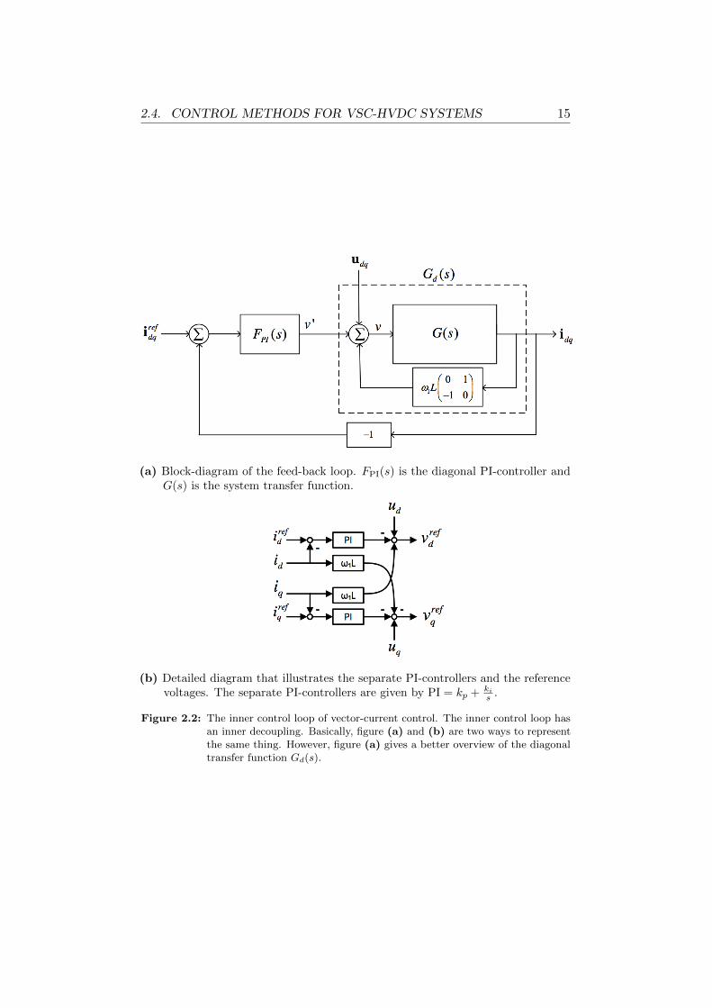
The transfer function in (2.13) is decoupled and can therefore be controlledwith a diagonal PI-controller, which means that the d and q components canbe controlled independently as two single-variable systems. An illustration ofthe decoupling is shown in figure 2.2. The PI-controller can be expressed as
FPI(s) = −(kp + ki
s 0
0 kp + kis
). (2.14)
2.4. CONTROL METHODS FOR VSC-HVDC SYSTEMS 15
(a) Block-diagram of the feed-back loop. FPI(s) is the diagonal PI-controller andG(s) is the system transfer function.
(b) Detailed diagram that illustrates the separate PI-controllers and the referencevoltages. The separate PI-controllers are given by PI = kp + ki
s .
Figure 2.2: The inner control loop of vector-current control. The inner control loop hasan inner decoupling. Basically, figure (a) and (b) are two ways to representthe same thing. However, figure (a) gives a better overview of the diagonaltransfer function Gd(s).
2.4. CONTROL METHODS FOR VSC-HVDC SYSTEMS 16
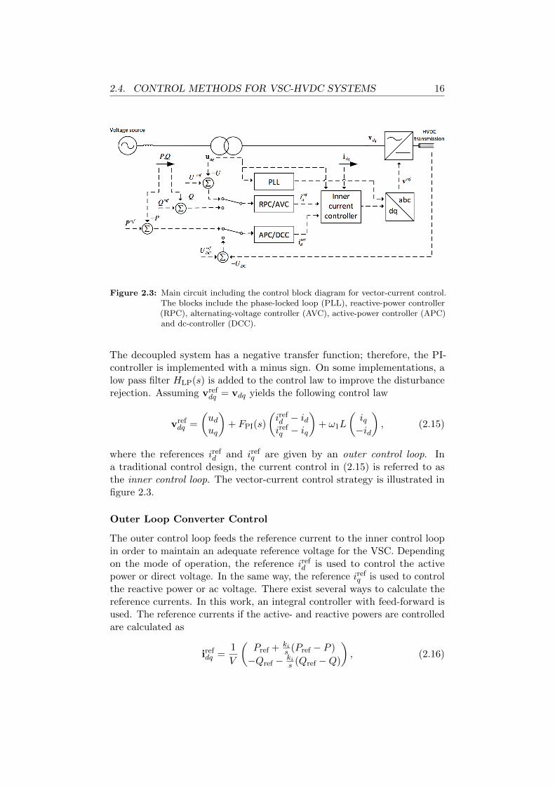
Figure 2.3: Main circuit including the control block diagram for vector-current control.The blocks include the phase-locked loop (PLL), reactive-power controller(RPC), alternating-voltage controller (AVC), active-power controller (APC)and dc-controller (DCC).
The decoupled system has a negative transfer function; therefore, the PI-controller is implemented with a minus sign. On some implementations, alow pass filter HLP(s) is added to the control law to improve the disturbancerejection. Assuming vref
dq = vdq yields the following control law
vrefdq =
(uduq
)+ FPI(s)
(irefd − idirefq − iq
)+ ω1L
(iq−id
), (2.15)
where the references irefd and irefq are given by an outer control loop. Ina traditional control design, the current control in (2.15) is referred to asthe inner control loop. The vector-current control strategy is illustrated infigure 2.3.
Outer Loop Converter Control
The outer control loop feeds the reference current to the inner control loopin order to maintain an adequate reference voltage for the VSC. Dependingon the mode of operation, the reference irefd is used to control the activepower or direct voltage. In the same way, the reference irefq is used to controlthe reactive power or ac voltage. There exist several ways to calculate thereference currents. In this work, an integral controller with feed-forward isused. The reference currents if the active- and reactive powers are controlledare calculated as
irefdq =1
V
(Pref + ki
s (Pref − P )
−Qref − kis (Qref −Q)
), (2.16)

2.4. CONTROL METHODS FOR VSC-HVDC SYSTEMS 17
where V = |vdq| =√v2d + v2q is the voltage magnitude at the converter
bridge.Recall that P = vdid + vqiq and Q = vqid − vdiq. If the voltage at the
converter bridge is aligned with the d axis and kept at 1 pu (i.e., vq = 0and vd = 1 pu), the currents can be expressed as id = P/vd = P andiq = −Q/vd = −Q. Therefore, a simpler controller instead of (2.16) couldbe
irefdq =
(Pref
−Qref
). (2.17)
However, the integral action from the controller in (2.16) helps to compen-sate for too abrupt power changes when the reference is changed. Also,the controller (2.17) needs the voltage constant and at its nominal value.Therefore, the controller from (2.16) is a preferable choice.
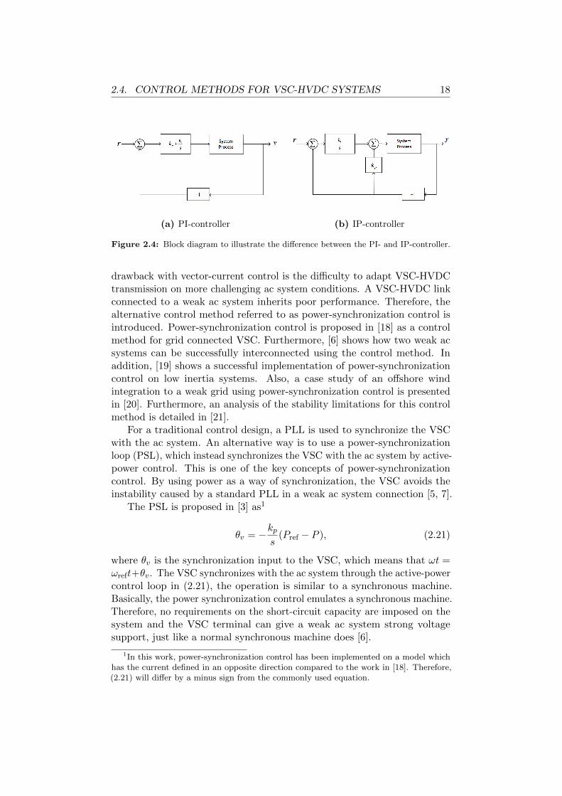
As an alternative to the traditional PI-controller, [17] explored the prop-erties of an IP-controller and showed some advantages compared to thePI-controller for implementations on dc drives. Figure 2.4 illustrates thedifference between a PI-controller and an IP-controller. The developedPSCAD model utilizes an IP-controller. The reference currents for direct-and alternating voltages in an IP-controller are calculated as
irefdq =
(kis (U ref
dc − Udc)− kpUdckis (U ref − U)− kpU
), (2.18)
where U = |udq| =√u2d + u2q is the voltage magnitude at the primary side
of transformer and Udc is the direct voltage. It is also possible to control thevoltage at the ac converter bridge instead of primary side of transformer byreplacing U with V . In order to improve disturbance rejection a low passfilter HLP(s) can be added for the controllers in (2.16) and (2.18).
In addition to (2.16) and (2.18), there exist two more control modes. Ifthe system is configured to control the active power and the ac voltage thereference currents are calculated as
irefdq =
(1V [Pref + ki
s (Pref − P )]kis (U ref − U)− kpU
), (2.19)
and if the system is configured to control the direct voltage and the reactivepower the reference currents are calculated as
irefdq =
(kis (U ref
dc − Udc)− kpUdc1V [−Qref − ki
s (Qref −Q)]
). (2.20)
2.4.2 Power-Synchronization Control
As already mentioned, there exists many real-life VSC-HVDC links wherevector-current control has been successfully applied. However, a major
2.4. CONTROL METHODS FOR VSC-HVDC SYSTEMS 18
(a) PI-controller (b) IP-controller
Figure 2.4: Block diagram to illustrate the difference between the PI- and IP-controller.
drawback with vector-current control is the difficulty to adapt VSC-HVDCtransmission on more challenging ac system conditions. A VSC-HVDC linkconnected to a weak ac system inherits poor performance. Therefore, thealternative control method referred to as power-synchronization control isintroduced. Power-synchronization control is proposed in [18] as a controlmethod for grid connected VSC. Furthermore, [6] shows how two weak acsystems can be successfully interconnected using the control method. Inaddition, [19] shows a successful implementation of power-synchronizationcontrol on low inertia systems. Also, a case study of an offshore windintegration to a weak grid using power-synchronization control is presentedin [20]. Furthermore, an analysis of the stability limitations for this controlmethod is detailed in [21].
For a traditional control design, a PLL is used to synchronize the VSCwith the ac system. An alternative way is to use a power-synchronizationloop (PSL), which instead synchronizes the VSC with the ac system by active-power control. This is one of the key concepts of power-synchronizationcontrol. By using power as a way of synchronization, the VSC avoids theinstability caused by a standard PLL in a weak ac system connection [5, 7].
The PSL is proposed in [3] as1
θv = −kps
(Pref − P ), (2.21)
where θv is the synchronization input to the VSC, which means that ωt =ωreft+θv. The VSC synchronizes with the ac system through the active-powercontrol loop in (2.21), the operation is similar to a synchronous machine.Basically, the power synchronization control emulates a synchronous machine.Therefore, no requirements on the short-circuit capacity are imposed on thesystem and the VSC terminal can give a weak ac system strong voltagesupport, just like a normal synchronous machine does [6].
1In this work, power-synchronization control has been implemented on a model whichhas the current defined in an opposite direction compared to the work in [18]. Therefore,(2.21) will differ by a minus sign from the commonly used equation.

2.4. CONTROL METHODS FOR VSC-HVDC SYSTEMS 19
An inner loop for converter control is not a necessary condition whenpower-synchronization control is used because the power is controlled di-rectly from the PSL and the alternating-voltage is controlled directly bythe VSC voltage. The work in [18] propose an integral controller that willmaintain a voltage of 1 pu with the alternating-voltage controller (AVC). Asan alternative, the IP-controller is implemented as
∆V =
(kis (Uref − U)− kpU
0
). (2.22)
It is possible to set vrefdq = ∆V if the inner loop of the converter control
is not used. However, there mainly exists two benefits in keeping the innerloop in (2.15): (i) it provides damping effects to poorly damped resonancesin ac systems, and (ii), it limits the valve current of the converter duringsevere ac system faults.
As previously discussed, the VSC needs to synchronize to the ac systemeither by the PLL or the PSL. In vector-current control mode, the convertercontrol use the PLL. In power-synchronization control mode, the convertercontrol use the PSL. In order to keep the same inner loop for both controlstrategies, the trick for power-synchronization control mode is to arrange a
current reference control so that irefdq =(irefd irefq
)Tin (2.15) yields a voltage
vector control law. This is achieved by
irefdq =1
kp[∆V +HHP(s)
(idiq
)−(uduq
)− ω1L
(iq−id
)] +
(idiq
), (2.23)
where HHP(s) is a high-pass filter for damping purposes and ∆V is given bythe AVC in (2.22).
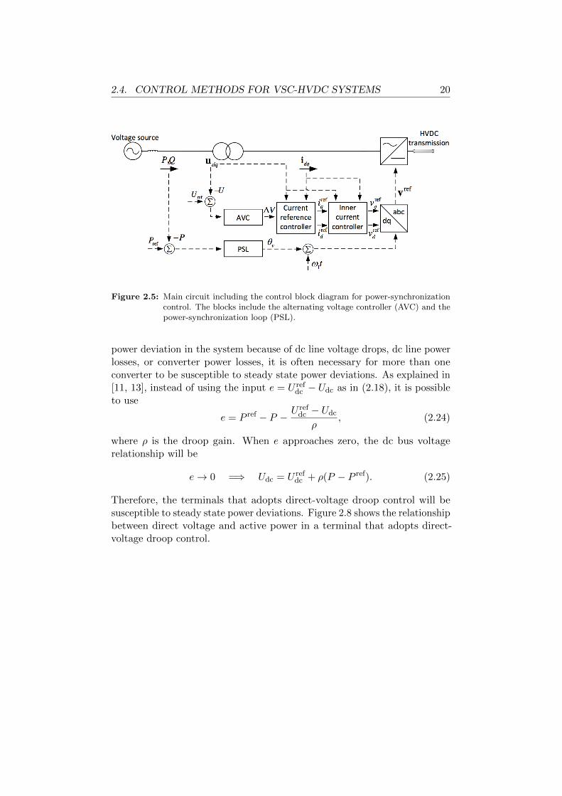
Figure 2.5 illustrates how power-synchronization control can be imple-mented.
2.4.3 Droop Control
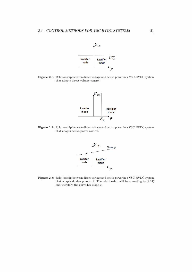
A thorough discussion about how droop control is implemented can be readabout in [11] and [13]. If a direct-voltage controller is implemented accordingto (2.18), the relationship between direct voltage and active power will beas shown in figure 2.6 (this is discussed in [13]). In the same way, if anactive-power controller is implemented according to (2.16), the relationshipwill be as in figure 2.7. As discussed in chapter 2, a terminal with direct-voltage control will be referred to as the dc slack-bus station and the otherstations as active-power controller stations. In such configuration, there willnot be any steady state power deviations in the power controlled at theVSC-HVDC terminals; the active power flow will be according to (2.8). Ifinstead the system adopts direct-voltage droop control the terminals willbe susceptible to steady state power deviations. If there is an unaccounted
2.4. CONTROL METHODS FOR VSC-HVDC SYSTEMS 20
Figure 2.5: Main circuit including the control block diagram for power-synchronizationcontrol. The blocks include the alternating voltage controller (AVC) and thepower-synchronization loop (PSL).
power deviation in the system because of dc line voltage drops, dc line powerlosses, or converter power losses, it is often necessary for more than oneconverter to be susceptible to steady state power deviations. As explained in[11, 13], instead of using the input e = U ref
dc − Udc as in (2.18), it is possibleto use
e = P ref − P −U refdc − Udc
ρ, (2.24)
where ρ is the droop gain. When e approaches zero, the dc bus voltagerelationship will be
e→ 0 =⇒ Udc = U refdc + ρ(P − P ref). (2.25)
Therefore, the terminals that adopts direct-voltage droop control will besusceptible to steady state power deviations. Figure 2.8 shows the relationshipbetween direct voltage and active power in a terminal that adopts direct-voltage droop control.
2.4. CONTROL METHODS FOR VSC-HVDC SYSTEMS 21
Figure 2.6: Relationship between direct voltage and active power in a VSC-HVDC systemthat adapts direct-voltage control.
Figure 2.7: Relationship between direct voltage and active power in a VSC-HVDC systemthat adapts active-power control.
Figure 2.8: Relationship between direct voltage and active power in a VSC-HVDC systemthat adapts dc droop control. The relationship will be according to (2.24)and therefore the curve has slope ρ.

Chapter 3
Implementation and Designin PSCAD
In this work, Simulink (an extension of Matlab) and PSCAD have been used tosimulate VSC-HVDC systems. Both Simulink and PSCAD are graphical toolswith a wide variety of built-in functions that can be assembled into completesystems. Particularly, Matlab Simulink contains the SimPowerSystemstoolbox, which is a physical modeling tool for electric power systems. WithSimPowerSystems and PSCAD, models for an entire electric power systemcan be built just as it would be assembled from physical components. ThePSCAD model developed in this work is based on a Cigre generic controlmodel developed in Simulink. This section will describe the structure of thePSCAD model.
3.1 Implementation Approach
There exist several ways to implement the proposed control strategies inPSCAD. The PSCAD control structure shall replicate the control structurefrom the Simulink model. Therefore, three suggestions for the PSCADimplementation are:
1) Synchronize Simulink to PSCAD by the built in PSCAD interface toSimulink.
2) Implement the model graphically.
3) Generate C code from the Simulink model and let PSCAD integratewith the C code during run-time.
Alternative 1) utilize a user-defined block in PSCAD, which specify thenecessary inputs and outputs, to interface with a Matlab/Simulink file. Inorder to ensure correct results, PSCAD proceeds only after the Simulinkmodule simulation is completed each time step. In other words, PSCADcalls Simulink, which runs a whole simulation and then returns the result to

3.2. PSCAD TERMINOLOGY 23
PSCAD. A demonstration of this implementation on HVDC systems can beread about in [22], where the authors discovered that a simulation durationof 2 s, took 30.5 s in PSCAD, 72.2 s in Simulink, and 12503.58 s when thePSCAD interface to Simulink was used. To avoid too lengthy simulationsalternative 1) has been left out in this thesis.
Alternative 2) was considered to be the easiest way to implement bothcontrols strategies. Therefore, the VSC-HVDC system was built up usingthis approach. However, for simulations using vector-current control it isnecessary that the models behaviors are similar. The author discoveredthat an implementation using alternative 3) yields a much more similarbehavior. Therefore, vector-current control has also been implemented usingalternative 3).
When the model was implemented using C code, each control componentwas generated piece-by-piece. This approach was preferable in order tofacilitate debugging. The first approach was to generate all of the code atonce for implementation. However, after several failures the author startedfrom the graphical implementation and replaced each component piece-by-piece, which ensured a functional model after each component exchange.Therefore, only the components that behave different between simulationplatforms have been exchanged from the graphical implementation.
Most of the blocks in Simulink have support for C code generation. Acomplete list of blocks that has support for C code generation can be foundin the help section of Matlab. After code generation, the logic operator blockencountered some troubles when all of the code was implemented at once.Within the Simulink model the logic operator outputs an integer (1 for trueand 0 for false), which is multiplicated with a real control signal. Withinthe generated C code this multiplication resulted in an integer value becausethe integers (1 or 0) from the logic operator became declared as integers inthe generated C code. This issue can either be because of wrong settingsor because of lack of support. However, it is possible to remove this blockbefore the generation is performed without lack of functionality. This blockis considered to behave in the same way no matter which simulation platformthat is used.
3.2 PSCAD Terminology
The terminology used when working in PSCAD is introduced in this section.Mainly four different terms will be used: components, definitions, instances,and modules.
Components
A component or block is basically a graphical representation of a device. Acomponent is the basic building block to construct models with PSCAD.

3.3. GRAPHICAL IMPLEMENTATION IN PSCAD 24
Components have inputs and outputs that can be linked together with othercomponents to form larger systems.
Modules
A module is a combination of other components with their own canvas. Incontrast to modules, regular components normally consist of a hard-codedscript. Modules can also contain other modules within their canvas.
Definitions
All components or modules are defined by a definition. Every aspect of thecomponent or module is defined in the definition. This can include graphicalappearance, connection nodes, input parameters and model code. Only onedefinition can exist for every unique component or module.
Instances
An instance is a graphical copy of the definition, and is normally what is seenand manipulated by the user. Each instance can have different parametersettings from other instances based on the same definition. All componentsand modules have a single definition, from which many instances can becreated. However, any design changes to a component definition will affectall instances.
3.3 Graphical Implementation in PSCAD
This section describes how the VSC-HVDC system is constructed graphicallyin PSCAD.
3.3.1 The Average Value Model
The converter in the PSCAD model is modeled with an average value model(AVM). The theory of the AVM is discussed in chapter 2. The dc side currentIdc is calculated with (2.5). The dc side current is composed of Ic and IL,which are calculated according to (2.1) and (2.6). The calculation of Icand IL in the PSCAD model is illustrated in figure 3.1. This calculationis performed within the module called subsystem shown in figure 3.2. Themodule called subsystem in figure 3.2 injects the currents Ic and IL into thedc grid with opposite directions according to (2.5).
The ac side voltage is calculated according to (2.1) in the bottom left offigure 3.2. The phase voltages are generated by three single-phase voltagesources.

3.3. GRAPHICAL IMPLEMENTATION IN PSCAD 25
Figure 3.1: Calculation of the current Ic and the current IL. The dc current Idc iscomposed of Ic and IL. The resistance that models the converter losses isset to R = 0.002.
Figure 3.2: The calculation of the outputs from the module called subsystem is shown infigure 3.1. The currents Ic and IL are injected in the dc grid with oppositedirections according to (2.5). The phase voltages are calculated with (2.1)and generated by three single-phase voltage sources.

3.3. GRAPHICAL IMPLEMENTATION IN PSCAD 26
Control direct voltage
Control power
Ac2ve power reference
Reac2ve power reference
Reac2ve power reference
Figure 3.3: Point-to-point connection, one side controls the active power and the otherside controls the direct voltage. It is possible to configure the control modulein a certain mode of operation by changing its parameters accordingly. Theactive- and reactive power references are controlled trough inputs to themodule. The direct voltage reference is set by a parameter within the module.
3.3.2 The Control Module
The control is implemented as a module in PSCAD. The module has thevoltages and currents on both side of the transformer as input and themodulation index mi, i ∈ 1, 2, 3 as output. It is possible to configure themodule in a certain mode of operation. For example, in a point-to-pointsystem, one instance may be configured to control the active power andanother instance may be configured to control the direct voltage. This isaccomplished by changing the parameters of the instances accordingly. Anillustration of this is shown in figure 3.3.
The inside of the module is shown in figure 3.4. Both vector-currentcontrol and power-synchronization control are included in the control module.Next, a description of each module within the control module are described.
Signal Calculation
After the three phase quantities have been transformed to αβ − coordinates,the power, voltages, and currents are calculated in the signal calculationmodule as shown in figure 3.5. The active- and reactive power are calculatedwith the voltage and current in the αβ − coordinates. Both the active- andreactive power is filtered through a low pass filter. As is shown in figure 3.5the ac voltage magnitude is calculated as
|vαβ| =√v2α + v2β. (3.1)

3.3. GRAPHICAL IMPLEMENTATION IN PSCAD 27
Inner current controller
Outer controller Signal calcula0ons
PSL
PLL
Voltage control & current reference control
αβ-‐transform
dq-‐transform
Figure 3.4: Inside of the control module, which includes an αβ−transform, dq−transform,signal calculation module, outer controller module, inner current controllermodule, PLL module, PSL module, voltage control and current referencecontrol module.
Note that both the alternating and direct voltages are also filtered througha low pass filter.
Inner Current Controller
The theory of the inner current controller is detailed in chapter 2. The insideof the module is shown in figure 3.6. It includes a decoupling that is necessaryaccording to (2.11). It also includes the two PI-controllers according to (2.14).Furthermore, it includes a limitation of the amplitude and a transformationback from the d and q axes to three phase quantities. The PI-controller isshown in figure 3.7. It includes a proportional gain kp and an integral withgain ki and also an anti-windup functionality.
The Outer Control Loop
As already discussed in chapter 2, the outer controller calculates a referencecurrent to be fed to the inner current controller. The system can operate ineither vector-current control mode or power-synchronization control mode.In either way, both control modes use the inner current controller. However,only if the system is set to vector-current control mode, the outer controllerdescribed in figure 3.8 is used. In power-synchronization control mode the

3.3. GRAPHICAL IMPLEMENTATION IN PSCAD 28
Low-‐pass filter
Low-‐pass filter
Low-‐pass filter
Low-‐pass filter
Low-‐pass filter
Figure 3.5: Inside of the signal calculation module. The active- and reactive power iscalculated and filtered through a low pass filter. The ac voltage magnitudesare also calculated and filtered through a low pass filter. The direct voltageis filtered through a low pass filter.
PI-‐controller
PI-‐controller
Amplitude limita3on
Transforma3on back to three-‐phase
quan33es
Figure 3.6: Inside of the inner current control module. The module includes a decoupling,PI-controllers, amplitude limitation, and transformation from d and q axesto three phase quantities. The PI-controller is shown in figure 3.7.

3.3. GRAPHICAL IMPLEMENTATION IN PSCAD 29
Figure 3.7: Inside of the PI-controller module. The module includes a proportional gainkp and an integral with gain ki. It also has an anti-windup functionality.
current reference is calculated within the current reference module describedin subsequent sections.
The outer control module includes two integral controllers with feed-forward as in (2.16). The implementation of the integral controller with feed-forward is shown in figure 3.9. It also includes an anti-windup functionality.One of the two integral controllers is for the active-power control and theother one is for the reactive-power control. In addition, both the active-powercontrol and the reactive-power control has a voltage control override thatensures an acceptable voltage level for both the ac and direct voltages. Thevoltage control override implementation is shown in figure 3.10.
The system can switch between active-power control and direct-voltagecontrol. It can also switch between reactive-power control and ac voltagecontrol. Both the direct voltage control and the ac voltage control useIP-controllers as in (2.18). The implementation of the IP-controller is shownin figure 3.11.
Furthermore, the droop control functionality, explained in chapter 2, isimplemented together with the direct-voltage control. If desired, it is possibleto switch of the droop control by changing the parameters of the controlmodule accordingly.
The PLL and PSL
Depending on the mode of operation, an instance of the control modulehas the possibility to switch between vector-current control and power-synchronization control. The PLL is implemented by using the standardPSCAD PLL component. The PSL is implemented as shown in figure 3.12according to (2.21). The PSL includes an integral with gain ki and a voltagecontrolled oscillator (VCO).

3.3. GRAPHICAL IMPLEMENTATION IN PSCAD 30
DC voltage override
Ac0ve power IP-‐controller
AC voltage override
Reac0ve power IP-‐controller
AC voltage controller
DC voltage controller
Droop control
Figure 3.8: Inside of the outer control loop module. The module includes two integralcontrollers with feed-forward, voltage control overrides, dc- and ac voltagecontrollers.
Figure 3.9: Implementation of the integral controller with feed-forward.
Figure 3.10: Voltage control override for the active- and reactive power. The voltagecontrol override is not active as long as the voltage is within an acceptablelevel.

3.3. GRAPHICAL IMPLEMENTATION IN PSCAD 31
Figure 3.11: Implementation of the IP-controller.
Figure 3.12: Inside of the PSL module. The PSL includes an integral with gain ki and avoltage controlled oscillator.
3.3. GRAPHICAL IMPLEMENTATION IN PSCAD 32
Voltage controller
(IP-‐controller)
High pass filter
Current reference calcula:on
High pass filter
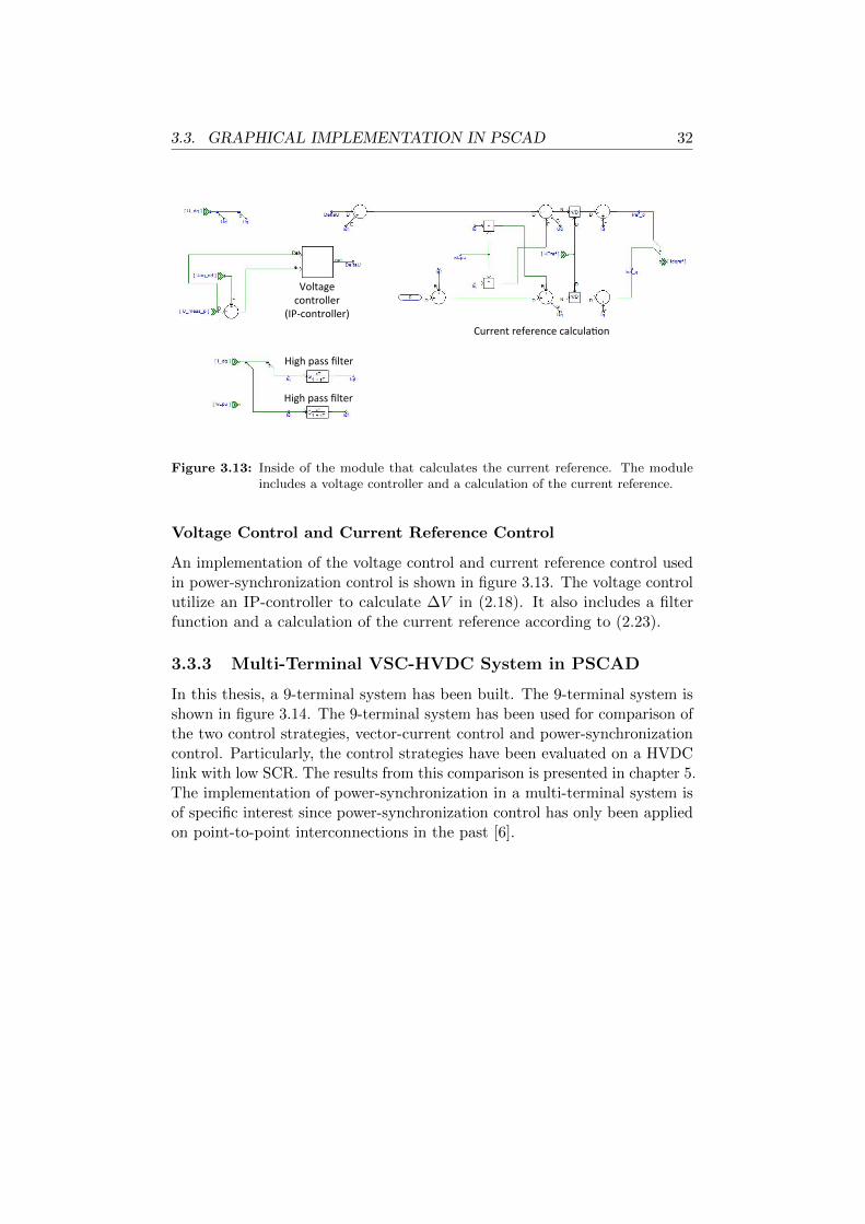
Figure 3.13: Inside of the module that calculates the current reference. The moduleincludes a voltage controller and a calculation of the current reference.
Voltage Control and Current Reference Control
An implementation of the voltage control and current reference control usedin power-synchronization control is shown in figure 3.13. The voltage controlutilize an IP-controller to calculate ∆V in (2.18). It also includes a filterfunction and a calculation of the current reference according to (2.23).
3.3.3 Multi-Terminal VSC-HVDC System in PSCAD
In this thesis, a 9-terminal system has been built. The 9-terminal system isshown in figure 3.14. The 9-terminal system has been used for comparison ofthe two control strategies, vector-current control and power-synchronizationcontrol. Particularly, the control strategies have been evaluated on a HVDClink with low SCR. The results from this comparison is presented in chapter 5.The implementation of power-synchronization in a multi-terminal system isof specific interest since power-synchronization control has only been appliedon point-to-point interconnections in the past [6].

3.3. GRAPHICAL IMPLEMENTATION IN PSCAD 33
VSC
VSC
VSC
VSC
VSC
VSC
VSC
VSC
VSC
DC link DC link
DC link
DC link
DC link
DC link
DC link
DC link
Figure 3.14: The multi-terminal VSC-HVDC system. The system consist of 9 terminals,7 voltage sources, and 3 loads. The system will be further explained inchapter 5.

3.4. CONTROL IMPLEMENTATION IN PSCAD USING CODEGENERATION 34
3.4 Control Implementation in PSCAD using CodeGeneration
This section explains an alternative way to implement the controls in PSCAD.Using this approach, the controls in PSCAD can be tailored to replicate thebehavior of Simulink very well.
As explained in section 3.1 (Implementation Approach), the implementa-tion was handled by exchanging piece-by-piece from the graphical implemen-tation. Figure 3.15 illustrates the order of how the controllers were generatedand implemented. First, the outer controller was generated, second theinner controller was generated, and finally the PLL was generated. Basically,everything in figure 3.8 was generated in the first step. In the second step,everything in figure 3.6 was generated except the limiter and transformationback to three-phase quantities. In the final step, the PLL from figure 3.4was generated. Also, four of the low-pass filter blocks from figure 3.5 weregenerated on each side of the point-to-point model. Only the low-pass filters,which were in use, were generated. The side that controls the direct voltagedoes not need to filter the active power and the side that controls the activepower does not need to filter the direct voltage. Therefore, eight low-passfilters were generated in total. The model was tested to ensure functionalitybetween each time the code was generated and implemented.
3.4.1 Simulink C Code Generation
In computing, C is a general-purpose programming language. The controlsfrom the generic Simulink model can be readily generated in C code. Thiscan be achieved using the built in Simulink Coder in Matlab. The SimulinkCoder generates C code from Simulink block diagrams, Stateflow charts, andMatlab functions. After the C code has been generated, it is possible to runand interact with the code outside Matlab and Simulink.
In this work, PSCAD has been used to execute the C code generatedfrom Simulink. PSCAD executes the C code on a fixed time-step interval.Therefore, it has been suitable to use the Embedded Coder, which extendsthe Simulink Coder in Matlab. When the Embedded Coder is used, theSimulink model is configured so it maintains a constant (fixed) step size andalso so it applies a fixed-step integration technique for computing the statederivative of the model. The fixed-step size used in this work is 20 ms. Someessential files generated from the Embedded Coder are shown in table 3.1.
As previously explained, the controller behavior depends on the values ofthe control parameters. It is possible to modify these values even after thecontroller has been generated in C code. Modifying the ModelName data.c
file changes the parameter values for the controller.One of the most important files generated from Simulink is the file that
contains the step function (called ModelName.c in table 3.1). The step

3.4. CONTROL IMPLEMENTATION IN PSCAD USING CODEGENERATION 35
Figure 3.15: In order to facilitate debugging, the code was generated in three main steps.First, the outer controller was generated. Second, the inner controller wasgenerated. Finally, the PLL was generated. Also the low pass filters weregenerated in C code, the low pass filters are not illustrated in this figure.
function should be executed each fixed time step during run-time in PSCAD.The files generated from the Embedded Coder in Simulink contain a
set of global variables along with the model step, initialize, and terminatefunctions. The global variables ModelName U and ModelName Y correspondsto the input and output structure of the model, respectively. These can beused to set the inputs prior to each execution of the step function and toreceive the outputs after each execution of the step function. Therefore, bythe use of a main execution file (ert main.c), the inputs are set, then thestep function is executed, and finally the outputs are set.
Code Generation and Execution of the Inner Control
The procedure to generate C code from Simulink is similar for any system.Therefore, the procedure is only illustrated for the inner control. This corre-sponds to code generation 2 from figure 3.15. The C code of the outer controlloop and the inner control loop are generated and implemented separately.The inner control loop of the Simulink model is shown in figure 3.16. Theinner control loop has 6 inputs and 2 outputs. The inputs are here called Ud,Uq, id, iq, i
refd , and irefq . The outputs are called d and q and represent the
voltages that will be transformed to three-phase quantities and convertedinto line voltages by the VSC. As recently explained, the generated C codefor the controller needs to be executed every 20 ms in PSCAD. Figure 3.17illustrates how the file, which is executed every 20 ms, can look like. Valuesare assigned for the inputs, the step function is executed, and values areassigned for the outputs. The code in figure 3.17 needs to be manually

3.4. CONTROL IMPLEMENTATION IN PSCAD USING CODEGENERATION 36
ert main.c Main file to execute step function
ModelName.c C file that contains the controller
ModelName data.c C file that assigns values to data structures
ModelName.h Header file that defines data structures
ModelName private.h Header file that defines data structures
ModelName types.h Header file that defines the model data structure
rtGetInf.c, rtGetNaN.c, Other C files and header files that are generatedrtwtypes.c, rtGetInf.h for the inner controller. These files serve artGetNaN.h, rtwtypes.h general purpose and can be used by other models.
Table 3.1: Files generated from the Simulink Coder.
written by the user.
3.4.2 Fortran Integration with C code
Fortran is a general-purpose programming language that is especially suitedfor numeric computations and scientific computing. Fortran can call existingcode that is written in another language. This is commonly referred to asmixed-language programming. In mixed-language programming, a routinewritten in Fortran can call a function written in C code. Mixed languageprogramming between these languages is relatively straightforward becauseof some key similarities between the languages.
PSCAD is a graphical front-end to EMTDC (Electromagnetic Transientsincluding DC) for creating models and analyzing results. EMTDC solvesdifferential equations in the time domain and calculates the solutions basedon a fixed time step. The blocks in PSCAD are actually Fortran code,which call for EMTDC code library to combine them into an executable file.Running this file, runs the simulation and the results can be picked up byPSCAD.
Figure 3.18 illustrates the Fortran code that can call the C procedure infigure 3.17. In C code, the arguments are passed either by value (passinga variable) or by reference (passing a pointer to a variable). It is necessaryto distinguish between these two when Fortran communicates with C. Incontrast to C, all arguments are passed by reference by default when aprocedure is called in Fortran. However, the code shown in figure 3.18anyway declares the arguments as reference attributes. If an argument shallbe passed as value, the arguments should be declared so in the code. Failureto do this will result in the values being treated as references and the programwill show incorrect results or run-time error.

3.4. CONTROL IMPLEMENTATION IN PSCAD USING CODEGENERATION 37
Figure 3.16: Simulink block diagram of the inner control loop. The inner control loopcontains two PI-controllers for each of the id and iq currents.

3.4. CONTROL IMPLEMENTATION IN PSCAD USING CODEGENERATION 38
1 #include <stdio.h>
2 #include "ModelName.h"
3 #include "rtwtypes.h"
4 void rt_onestep(double* Ud, double* Uq, double* d,
5 double* q, double* Ivq, double* Ivd,
6 double* Id_ref,double* Iq_ref)
7
8 ModelName_U.I_ref_q=*Iq_ref;
9 ModelName_U.I_ref_d=*Id_ref;
10 ModelName_U.Iv_d=*Ivd;
11 ModelName_U.Iv_q=*Ivq;
12 ModelName_U.U_q=*Uq;
13 ModelName_U.U_d=*Ud;
14 ModelName_step();
15 *Id=ModelName_Y.d;
16 *Iq=ModelName_Y.q;
17
Figure 3.17: The main function, which is manually written in C code. The code assignvalues to the inputs and outputs along with the execution of the stepfunction.
3.4.3 Linking a library to PSCAD
In PSCAD, components can be custom designed by Fortran code. Thecomponent wizard is used in order to create such component. This sectiondescribes how to create a component in PSCAD, which can be linked tothe C code generated from Simulink. Therefore, the component will inheritthe same functionality as the desired controller block in Simulink. Thecomponent can be created with a single line of Fortran code calling a Fortransubroutine such as in figure 3.18. The code contained in the component forcalling the subroutine is listed in figure 3.19.
Additionally library (.lib) and object (.obj) files can be linked in PSCAD.Therefore, all C and Fortran files are compiled into one library file that islinked to PSCAD. The procedure to compile all files is lengthy. Therefore,this is achieved with a bash script. The following text of this chapter describeshow to compile the inner and outer controller of a point-to-point model.
Unfortunately, it is not possible to use multiple instances of the compo-nents that can call a C function in PSCAD. Therefore, two inner controllers,and two outer controllers are generated from Simulink. In the subsequenttext, these are called inn1, inn2, out1, and out2. Simulink automaticallycreates a folder named ModelName ert shrlib rtw for each controller. Mod-elName here represents the controller name (e.g. inn1, inn2, out1, and out2).

3.4. CONTROL IMPLEMENTATION IN PSCAD USING CODEGENERATION 39
1 SUBROUTINE FUN(Ud,Uq,d,q,Ivq,Ivd,Id_ref,Iq_ref)
2 REAL Ud,Uq,d,q,Ivq,Ivd,Id_ref,Iq_ref
3 INTERFACE
4 SUBROUTINE RT_ONESTEP (Ud,Uq,d,q,Ivq,Ivd,Id_ref,Iq_ref)
5 !DEC$ ATTRIBUTES C :: RT_ONESTEP
6 !DEC$ ATTRIBUTES REFERENCE :: Ud
7 !DEC$ ATTRIBUTES REFERENCE :: Uq
8 !DEC$ ATTRIBUTES REFERENCE :: d
9 !DEC$ ATTRIBUTES REFERENCE :: q
10 !DEC$ ATTRIBUTES REFERENCE :: Ivq
11 !DEC$ ATTRIBUTES REFERENCE :: Ivd
12 !DEC$ ATTRIBUTES REFERENCE :: Id_ref
13 !DEC$ ATTRIBUTES REFERENCE :: Iq_ref
14 REAL Ud,Uq,d,q,Ivq,Ivd,Id_ref,Iq_ref
15 END SUBROUTINE
16 END INTERFACE
17 CALL RT_ONESTEP(Ud,Uq,d,q,Ivq,Ivd,Id_ref,Iq_ref)
18 END
Figure 3.18: Fortran code which calls the C function in figure 3.17. Note the call of theC procedure on line 17.
1 CALL FUN($Ud,$Uq,$d,$q,$Ivq,$Ivd,$Id_ref,$Iq_ref)
Figure 3.19: Single line Fortran code in the PSCAD module which calls the subroutinein Fig 3.18.

3.4. CONTROL IMPLEMENTATION IN PSCAD USING CODEGENERATION 40
The folder contains all C code files listed in figure 3.1. Further, the bashscript is placed in a manually created folder called interface, placed in thesame directory as automatically generated folders from Simulink. The bashscript is listed in figure 3.20. The main bash script executes one additionallybash script for each controller. These additionally bash scripts are locatedin each of the Simulink generated folders. The bash script for controllerinn1 is listed in figure 3.21. In the main bash script shown in figure 3.20,some C code files are compiled on row 25 and 26. Further, some Fortranfiles are compiled on row 29 and 30. The files compiled here are listed in thetext files clist.txt and flist.txt, respectively. These files can be used incommon by all controllers, i.e., the files listed in the bottom of table. 3.1. TheFortran files contains the Fortran code described in figure 3.18, one Fortranfile is needed for each controller. Finally, everything is put together into acontrol.lib file. This is achieved on line 33 in the main bash script. Thecontrol.lib file can easily be linked in PSCAD. After the C and Fortranfiles have been linked, the modules in PSCAD will execute the correspondingC function.
For the tests performed in chapter 4, also the PLL and low pass filtershave been implemented using C code. This was done in order to mimic thebehavior of the Simulink model in more detail.
3.4.4 Overall Integration for the Code Implementation
The previous sections describe how to generate the C code of the controllersfrom Simulink and implement them in PSCAD. To illustrate the whole pro-cess, a flowchart is shown in figure 3.22. The upper left of the flowchart showshow the code is automatically generated form Simulink. The automaticallygenerated files here are those shown in table 3.1. The ert main.c file intable 3.1 needs to be manually written or modified by the user. Therefore,the ert main.c file is shown in the upper right of the flowchart, along withthe manually written Fortran files, which has the structure explained infigure 3.18.
The process to merge the automatically generated and manually writtenfiles into a control.lib is lengthy. Therefore, the files are merged togetherwith a bash script as was shown in figure 3.20. Bottom of the flowchartillustrates how the control.lib file finally is linked together with PSCADduring run-time.
The procedures within the grey box in figure 3.22 needs to be manuallywritten or modified by the user. This is the most time consuming andcomplicated part regarding the C code implementation. Particularly, theprocedure needs to be repeated for each component that calls any C codebecause multiple instances are not supported. There exists a possibility towrite a script that automatically writes the Fortran and C code needed foreach module. However, this is considered to be out of the scope for this

3.4. CONTROL IMPLEMENTATION IN PSCAD USING CODEGENERATION 41
1 @echo off
2
3 echo Compiling control library
4
5 cd ..
6
7 cd inn1_ert_shrlib_rtw
8 call makefile.bat
9 cd ..
10
11 cd inn2_ert_shrlib_rtw
12 call makefile.bat
13 cd ..
14
15 cd out1_ert_shrlib_rtw
16 call makefile.bat
17 cd ..
18
19 cd out2_ert_shrlib_rtw
20 call makefile.bat
21 cd ..
22
23 cd interface
24
25 cl -O2 -c -I"C:\Program Files (x86)\
26 Microsoft Visual Studio 9.0\VC\Include" @clist.txt
27 if not %errorlevel% == 0 goto error
28
29 ifort -O2 -c -free -I"C:\Program Files (x86)\
30 Microsoft Visual Studio 9.0\VC\Include" @flist.txt
31 if not %errorlevel% == 0 goto error
32
33 lib /OUT:control.lib @objlist.txt
34 if not %errorlevel% == 0 goto error
35
36
37 goto end
38
39 :error
40 pause
41 :end
Figure 3.20: Main batch script to compile all Fortran and C files into a common libraryfile.

3.4. CONTROL IMPLEMENTATION IN PSCAD USING CODEGENERATION 42
1 @echo off
2
3 echo Compiling inn1_ert_shrlib_rtw..
4
5 cl -O2 -c -I"C:\Program Files (x86)\
6 Microsoft Visual Studio 9.0\VC\Include" @filelist.txt
7 if not %errorlevel% == 0 goto error
8
9 lib /OUT:inn1.lib @objlist.txt
10 if not %errorlevel% == 0 goto error
11
12 goto end
13 :error
14 pause
15 :end
Figure 3.21: Additionally bash script within each of the generated folders from Simulink.The script shown is for controller inn1.
thesis. A similar script is illustrated in [23]; the script automatically writescode, which can be used with Simulink and hardware components.
The grey box can be considered as a customized interface in order toget the C code implementation to work. This interface is rather difficult tobuild and maintain. It also lacks generality. There exists a standardizedinterface to be used in computer simulations, called the functional mock-upinterface (FMI) [24]. This tool is an independent standard to support bothmodel exchange and co-simulation of dynamic models using a combination ofxml files and compiled C code. With such interface there is no need for anymanual or automatic script writing. Unfortunately, PSCAD lacks support forthis interface. Hopefully, the future will see more of standardized interfacesthat work between a broader set of simulation platforms.

3.4. CONTROL IMPLEMENTATION IN PSCAD USING CODEGENERATION 43
Simulink model
Automatic code generation
Scripts written and modified by user
Model.c
Model.h
Model_data.c
Model_data.h
ert_main_inn1.c
Inn1.f
Inn2.f
out1.f
out2.fert_main_out2.c
Makefile.bat
Execution of bash scripts which compiles the Fortran and C code
ert_main_out1.c
ert_main_inn2.c
Makefile.bat
Control.lib
PSCAD simulation Control.lib
Linking library file at run-time
Embedded Coder
This grey box contains all lengthy procedures, which
are not handled automatically
Figure 3.22: The flowchart describes how the control.lib file is generated and linked as alibrary file in PSCAD during run-time. The grey box contains all procedures(script writing and compilation), which are not handled automatically. Theother boxes are more or less automated.

3.4. CONTROL IMPLEMENTATION IN PSCAD USING CODEGENERATION 44
3.4.5 Scalability of the Proposed Implementation
Scalability is the ability of a computer application or product to functionwell as it is changed in volume or size [25]. In other words, scalability is theconcept of a system to accommodate an increasing number of elements orobjects. Therefore, scalability is often a desirable attribute for almost anysystem.
In a multi-terminal VSC-HVDC system, scalability becomes an importantissue when the number of converters increases. In PSCAD, it is normallypossible to use multiple instances of modules. Therefore, it is easy to extenda point-to-point system to any number of terminals linked together by a dcgrid. A multi-terminal VSC-HVDC system can be built by a copy and pasteprocedure. Normally, the limiting factor will be the increase in simulationtime when the system increase in complexity.
One of the most major drawbacks with the C code implementation inPSCAD is the lack of possibility to use multiple instances of modules. Thisconstraint forces the user to go through all the relevant steps in the previoussections for each terminal. This is a rather lengthy procedure compared tothe simple copy and paste procedure. How lengthy this procedure will bedepends on the number of inputs and outputs of the system, because eachsignal needs some lines of code when the Fortran and C code scripts aremade.
On the other hand, if the system in Simulink is complex, only has a fewset of inputs and outputs, and only a few instances of the same module willbe used. Then, this approach may be very appealing. An illustration of whenthe approach should be good or bad is shown in figure 3.24 and figure 3.23.The illustration in figure 3.24 is mainly because of the time it takes to writethe C and Fortran code for each module. If this is done automatically, thefocus will be on figure 3.23. There will be a trade-off between the number ofmodules, the total number of inputs and outputs, and the complexity of thesystem within the module.
As previously discussed, there exist no script that automatically writesthe Fortran and C code for the customized interface shown in figure 3.22.Therefore, with n modules, i inputs, and j outputs, there will be n(i+ j)/2more steps to consider in the Fortran and C code in comparison to onemodule with one input and one output.
The example in section 3.4.1 illustrates how the inner controller is ex-tracted in C code. The inner controller has in total 8 inputs and outputswhile the complexity is rather simple. The inner controller consists of twoPI-controllers and an additional decoupling term. Therefore, it can be builtgraphically rather quickly in PSCAD. The author has found that it is easier toconstruct such module graphically. Particularly, it will facilitate to constructmodules graphically if several modules are used in the project.

3.4. CONTROL IMPLEMENTATION IN PSCAD USING CODEGENERATION 45
Complexity of the system within the module
Number of inputs and outputs of
the module
Good to implement C code in this case
Consider to construct the module
graphically in this case
Figure 3.23: Illustration of a good and bad scenario when to use C code from Simulinkto construct a module. Note that the y axis denotes the total number ofinputs and outputs.
Complexity of the system within the module
Number of modules in the
project
Good to implement C code in this case
Consider to construct the module
graphically in this case
Figure 3.24: Illustration of a good and bad scenario when to use modules of C code tobuild up a project. In contrast to figure 3.23, note that the y axis denotesthe number of modules within the whole project.

Chapter 4
Controller PerformanceComparisons and Analysis
This chapter compare and analyze the different software implementations ofvector-current control. The Simulink model will be considered as a referencefor these comparisons. Therefore, comparisons to the Simulink model arefirst performed in order to ensure that deviations are not too large. Further,comparisons are performed with the manufacturer’s black-box model. Thecontrollers are compared using the eight test scenarios presented in figure 4.1.Comparisons with the Simulink model are performed on the rectifier side,while comparisons with the manufacturer’s black-box model are performedon both rectifier and inverter side. The comparisons are performed on apoint-to-point link.

4.1. METHODOLOGY 47
1) Step of the active-power controller by 30%.
2) Step of the reactive-power controller by 30%.
3) Three-phase fault at the primary side of transformer during 100 mswith 10% remaining voltage.
4) Three-phase fault at the primary side of transformer during 100 mswith 30% remaining voltage.
5) Three-phase fault at the primary side of transformer during 100 mswith 70% remaining voltage.
6) Single-phase fault at the primary side of transformer during 100 mswith 10% remaining voltage.
7) Single-phase fault at the primary side of transformer during 100 mswith 30% remaining voltage.
8) Single-phase fault at the primary side of transformer during 100 mswith 70% remaining voltage.
Figure 4.1: Eight test scenarios used for controller performance comparisons.
4.1 Methodology
The comparisons are performed both graphically and numerically. Thissection describes the methodology of how the numerical comparisons areperformed. It also describes how the system was configured during the testscenarios in figure 4.1.
4.1.1 Numerical Comparisons
For the numerical comparison, the root mean square (RMS) is used. Thenumerical comparisons are always performed between two software or con-troller implementations. It is the active- and reactive power that is comparedbetween implementations. Therefore, the RMS value is calculated accordingto
XRMS =
√1
n[(x1 − y1)2 + (x2 − y2)2 + · · ·+ (xn − yn)2]), (4.1)
where xi is the discrete measurement point at time ti for software/controllerimplementation (i), and yi is the discrete measurement point at time tifor software/controller implementation (ii). That is, if x(t) and y(t) arecontinues functions of the active- or reactive power, then x(ti) = xi andy(ti) = yi, where t1 < . . . < ti < . . . < tn−1 < tn. The RMS value iscalculated on an interval of 1.5 s divided into 15000 measurement points (i.e.,

4.2. CONTROLLER PERFORMANCE COMPARISONS 48
ti+1 − ti = 0.0001). The interval is spread over a duration of the particulartest scenario starting 0.5 s before the test is performed. In other words, if afault is injected at t = 1 s, then t1 = 0.5 s and t15000 = 1.9999 s.
4.1.2 Fault Impedance and System Configuration
The generators voltage is set to U = 275∠0 kV and they operate at 50 Hz.Each generator has an impedance of Zgen = 16.9∠85Ω, which yields ashort-circuit capacity of approximately Sac = 4500∠85MVA. The HVDClink is set to 300 MW. It is possible to calculate a fault impedance Zf thatyields a remaining voltage of 10%, 30%, or 70% for each fault scenario. Letn denote the fraction of remaining voltage during fault (i.e., n = 0.1⇒ 10%remaining voltage, n = 0.3⇒ 30% remaining voltage, and n = 0.7⇒ 70%remaining voltage). The calculation become as follows.
If (Zgen + Zf ) = U =⇒
IfZgen = nUIfZf = (1− n)U
(4.2)
It follows that
Zgen = |U |2S∗ac
Zgen
Zf= n
1−n
=⇒ Zf =
|U |2
S∗ac
(n− 1)
n=|U |2
|Sac|(n− 1)
n∠85, (4.3)
where S∗ac denotes the complex conjugate of Sac. Using the fault impedanceZf from equation 4.3 yields the voltage curves in appendix A. The voltagecurves of each fault scenario are very similar between systems. Therefore,appendix A only demonstrates the plots from Simulink.
4.2 Controller Performance Comparisons
Before the comparison between the PSCAD model and the manufacturer’sblack-box model, the comparisons between the two PSCAD implementationsand Simulink model are performed. The parameters used in the Simulink andPSCAD models for this comparisons are listed in table 4.1. The eight testscenarios from figure 4.1 are performed. Figure 4.2 illustrates a comparisonof the active power during a three-phase fault with 10% remaining voltage.For the same test scenario, the reactive power is shown in figure 4.3. All plotsfrom comparisons between the graphical implementation and the Simulinkmodel are shown in appendix B, while all plots from comparisons betweenthe C code implementation and the Simulink model are shown in appendix C.Further, table 4.2 and 4.3 lists the RMS measurements calculated accordingto (4.1). In addition to active- and reactive power measurements, appendix Band C also illustrates how the current |idq| and the reference currents irefd andirefq are influenced during each test scenario. Table 4.2 and 4.3 also list inwhich figure from appendix the power and current measurements are found.

4.2. CONTROLLER PERFORMANCE COMPARISONS 49
Controller Parameter value
Inner current loop kp 0.4Inner current loop ki 85
Direct voltage control kp 6Direct voltage control ki 200
Outer control loop active power ki 15Outer control loop reactive power ki 15
Voltage control override ac kp 10Voltage control override ac ki 3Voltage control override dc kp 10Voltage control override dc ki 3
Table 4.1: Parameters used when comparing the Simulink model to the PSCAD models.
4 4.1 4.2 4.3 4.4 4.50
0.2
0.4
0.6
0.8
1
Time [s]
P [p
u]
SIMULINKC CodeGraphically
Figure 4.2: Illustration of the active power during a three-phase fault with 10% remainingvoltage. This corresponds to scenario 3) from figure 4.1.

4.2. CONTROLLER PERFORMANCE COMPARISONS 50
4 4.1 4.2 4.3 4.4 4.5−0.85
−0.4
0
0.4
Time [s]
Q [p
u]
SIMULINKC CodeGraphically
Figure 4.3: Illustration of the reactive power during a three-phase fault with 10% re-maining voltage. This corresponds to scenario 3) from figure 4.1.
Test scenario 1 2 3 4
PRMS 0.0030 0.0144 0.0435 0.0386QRMS 0.0143 0.0026 0.0628 0.0573
Power measurement in figure B.1 B.3 B.5 B.7Current measurement in figure B.2 B.4 B.6 B.8
Test scenario 5 6 7 8
PRMS 0.0421 0.0557 0.0542 0.0208QRMS 0.0513 0.0587 0.0555 0.0081
Power measurement in figure B.9 B.11 B.13 B.15Current measurement in figure B.10 B.12 B.14 B.16
Table 4.2: RMS calculations according to (4.1). The calculations regards the graphicalimplementation compared to the Simulink model. The RMS values arecalculated for the active- and reactive power. Also, the references to relevantfigures in appendix are listed.

4.3. CONTROLLER PERFORMANCE ANALYSIS AND RESULTS 51
Test scenario 1 2 3 4
PRMS 0.0076 0.0003 0.0198 0.0125QRMS 0.0003 0.0002 0.0031 0.0020
Power measurement in figure C.1 C.3 C.5 C.7Current measurement in figure C.2 C.4 C.6 C.8
Test scenario 5 6 7 8
PRMS 0.0061 0.0061 0.0062 0.0063QRMS 0.0003 0.0019 0.0011 0.0004
Power measurement in figure C.9 C.11 C.13 C.15Current measurement in figure C.10 C.12 C.14 C.16
Table 4.3: RMS calculations according to (4.1). The calculations regards the C codeimplementation compared to the Simulink model. The RMS values arecalculated for the active- and reactive power. Also, the references to relevantfigures in appendix are listed.
4.3 Controller Performance Analysis and Results
To this end, no statement has been made on how well the curves match tothe Simulink model for each PSCAD implementation. A glance at figure 4.2and 4.3 gives a hint about that the C code implementation provides the bestmatch. The conclusion from figures in appendix and from RMS calculationsare that the curves match much better for the C code implementation. Themeans (here denoted X) of all active- and reactive power RMS measurementsare significantly lower for the C code implementation compared to thegraphical implementation. The means for the graphical implementation are
PgrRMS = 0.0340,
QgrRMS = 0.0388.
Further, the means for the C code implementation are
PccRMS = 0.0081,
QccRMS = 0.0012.
It follows that the active power match is
PgrRMS
PccRMS
≈ 4
times better for the C code implementation. The reactive power match is
QgrRMS
QccRMS
≈ 33

4.4. BLACK-BOX MODEL COMPARISONS 52
times better. Note that these calculations are only representative for thespecific test scenarios in figure 4.1, here tested on the rectifier side. Otherscenarios might turn out different. In addition to the active- and reactivepower measurements, the variables irefd , irefq , and |idq| have almost no differencefor the C code implementation. This can be seen from the plots in appendix C.Therefore, the C code implementation is used for comparisons with themanufacturer’s black-box model.
4.4 Black-Box Model Comparisons
The comparisons are performed between the C code implementation anda manufacturer’s black-box model in PSCAD. The black-box protects anyintellectual property invested in the design by the manufacturer. Therefore,the tests are performed without any knowledge about the control implemen-tation within the black-box. For example, components like shunt reactorsand dc link capacitors are unknown. Also, control strategies and controltuning are unknown. The manufacturer’s black-box model might also takemore things into consideration (e.g., it is not modeled with an AVM).
The parameters used for the C code implementation are listed in table 4.4.These are tuned in order to have a better match to the manufacturer’s black-box model. All eight test scenarios from figure 4.1 are performed on therectifier side. Further, test scenarios 3 to 8 are performed on the inverter side.Figure 4.4 illustrates a comparison of the active power during a single-phasefault with 10% remaining voltage at rectifier side. For the same test scenario,the reactive power is shown in figure 4.5. Appendix D presents all figuresfrom comparisons.
Table 4.5 lists all RMS calculations and figure references for the rectifierside, while table 4.6 lists all RMS calculations and figure references for theinverter side. The mean value calculations from the RMS values are
PgrRMS = 0.1078,
QgrRMS = 0.0460.

4.4. BLACK-BOX MODEL COMPARISONS 53
0.15 0.2 0.25 0.3 0.35 0.4 0.45 0.5−0.5
0
0.5
1
1.5
2
Time [s]
P [
pu]
Manufacturer’s black−box modelGeneric control
Figure 4.4: Illustration of the active power during a single-phase fault with 10% remainingvoltage. This corresponds to scenario 6) from figure 4.1.
0.15 0.2 0.25 0.3 0.35 0.4−0.2
−0.1
0
0.1
0.2
0.3
Time [s]
Q [p
u]
Manufacturer’s black−box modelGeneric control
Figure 4.5: Illustration of the reactive power during a single-phase fault with 10% re-maining voltage. This corresponds to scenario 6) from figure 4.1.
Controller Parameter value
Inner current loop kp 0.4Inner current loop ki 85
Direct voltage control kp 6Direct voltage control ki 200
Outer control loop active power ki 15Outer control loop reactive power ki 15
Voltage control override ac kp 0.1Voltage control override ac ki 0.1Voltage control override dc kp 0.1Voltage control override dc ki 0.1
Table 4.4: Parameters used when the C code implementation is compared with realisticcontrol performance results from industry.

4.4. BLACK-BOX MODEL COMPARISONS 54
Test scenario 1 2 3 4
PRMS 0.0715 0.0028 0.1134 0.1008QRMS 0.0110 0.0642 0.0755 0.0357
Power measurement in figure D.1 D.2 D.3 D.4
Test scenario 5 6 7 8
PRMS 0.0925 0.0719 0.0528 0.0784QRMS 0.1048 0.0217 0.0206 0.0180
Power measurement in figure D.5 D.6 D.7 D.8
Table 4.5: RMS calculations according to (4.1). The calculations regards the C codeimplementation compared to the manufacturer’s black-box model. The RMSvalues are calculated for the active- and reactive power on the rectifier side.Also, the references to relevant figures in appendix are listed.
Test scenario 3 4 5
PRMS 0.2000 0.1554 0.1308QRMS 0.0561 0.0398 0.1254
Power measurement in figure D.9 D.10 D.11
Test scenario 6 7 8
PRMS 0.1593 0.1518 0.1274QRMS 0.0243 0.0246 0.0217
Power measurement in figure D.12 D.13 D.14
Table 4.6: RMS calculations according to (4.1). The calculations regards the C codeimplementation compared to the manufacturer’s black-box model. The RMSvalues are calculated for the active- and reactive power on the inverter side.Also, the references to relevant figures in appendix are listed.

Chapter 5
Power-SynchronizationControl Analysis
This chapter summarize the main results presented in [8]. In particular, itis demonstrated how one terminal in a dc grid is connected to a very weakac system by using power-synchronization control. The ac system is weakbecause of the interconnecting lines and the conditions under which they areconnected. Thus far, power-synchronization control has only been applied topoint-to-point interconnections [6]. In this chapter, power-synchronizationcontrol is implemented in a multi-terminal VSC-HVDC system.
First the dc grid test system is described. Then, comparisons betweencontrol strategies are carried out.
5.0.1 The DC Grid Test System
The dc grid test system used in this work is based on the Cigre dc grid testsystem and therefore, it has the same topology. In this section, the dc gridtest system is described. The dc grid test system used for simulations isshown in figure 5.1. A description of the components used in figure 5.1 isshown in figure 5.2. There exist nine terminals in the system, marked in therange of A to I. In this experiment, converter station A is set to both vectorcurrent control mode and power-synchronization control mode. The otherconverter stations are always set to vector current control mode. Simulationsare performed with different references of the active-power controller forconverter station A. The control mode and active-power references of all theconverter stations are listed in table 5.1. Further, the line-to-line voltagesand the loads connected close to each converter are listed in table 5.2. All theHVDC links have a rated power of 1000 MW and all the generators operateat 50 Hz.
As described in figure 5.2, the system has different types of power lines.Some of the power lines are modeled using the PSCAD tower transmissionline models, and the others are modeled using simple pi-sections. Particularly,

56
Figure 5.1: The Cigre dc grid test system used for simulations.
Figure 5.2: Description of the components used in figure 5.1.
converter station A is considered. Both lines that connects converter stationA has a series resistance of 65 Ω and an inductance of 0.7 H. Therefore, eachline has an impedance of approximately 229 Ω.

57
Converter station Control mode Active-power reference
A Active-power Modified by user
B Active-power −1 pu
C Droop dc 0.2 pu
D Droop dc −0.3 pu
E Active-power −0.5 pu
F Active-power 0.4 pu
G Active-power 0.2 pu
H Active-power 0.2 pu
I Active-power 0.2 pu
Table 5.1: Controller data of all the converter stations
Converter station Line-to-line voltage Load close to converter
A 380 kV No load
B 380 kV 600 MW, PF = 0.9 lagging
C 380 kV 900 MW, PF = 0.9 lagging
D 380 kV 1500 MW, PF = 0.9 lagging
E 155 kV No load
F 155 kV No load
G 155 kV No load
H 155 kV No load
I 155 kV No load
Table 5.2: Voltage and load data of all the converter stations
5.1. INTERCONNECTION OF A WEAK AC SYSTEM 58
5.1 Interconnection of a Weak AC System
As previously discussed, [4] presents a way to measure the ac system strengthin terms of the short-circuit ratio (SCR). The SCR is calculated as
SCR =SacPdc
, (5.1)
where Sac is the short-circuit capacity of the ac system and Pdc is the ratedpower of the HVDC link. The strength of the ac system is from [4] definedas:
- Strong system, if the SCR is greater than 3.0.
- Weak system, if the SCR is between 2.0 and 3.0.
- Very weak system, if the SCR is lower than 2.0.
Consider converter station A, which has an ac bus in connection to a buswith a stiff voltage source and a bus connecting converter station D. In thissection, the SCR of the ac system connecting converter station A is estimated.Furthermore, simulations during a step response of the active-power controllerand during a three-phase fault are presented.
5.1.1 Estimation of the Short-Circuit Ratio
An estimation of the maximum SCR of the ac system in connection toconverter station A is performed to simplify the calculations. The maximumshort-circuit capacity at converter station A can be estimated as
Smaxac = 2
(380 kV)2
229 Ω≈ 1260 MVA, (5.2)
where a multiplication by 2 is performed because there are two interconnectinglines. Thus, when the rated power of the HVDC link is 1000 MW, themaximum SCR of the ac system is not greater than
SCR ≤ Smaxac
Pdc=
1260 MVA
1000 MW= 1.26. (5.3)
5.1.2 Step Response of the Active-Power Controller
The first test of power-synchronization control is a step response of theactive-power controller. Using vector current control, the authors of [5] wereable to achieve a maximum power transfer of 0.4 pu when only one of theconverter stations had a SCR of 1.0 in a point-to-point link. Figure 5.3illustrates that converter station A can maintain stable operation duringa step response from 0.1 pu to 0.3 pu of the active-power controller whenvector current control is used. At present, the thesis author is not able to

5.1. INTERCONNECTION OF A WEAK AC SYSTEM 59
achieve stable operation of converter station A during a step response from0.3 pu to 0.54 pu using vector current control on converter station A.
Figure 5.4 shows that it is possible to achieve a step response from 0.3 puto 0.7 pu using power-synchronization control in the multi-terminal VSC-HVDC system. The step response of the active-power controller is appliedat t = 0.1 s at converter station A.
5.1.3 Three-Phase Fault at the Bus of Converter A
The second test of power-synchronization control is to apply a three-phasefault at the bus that connects converter station A to the ac grid. Theactive-power measurement during the fault is shown in figure 5.5. Note thatconverter station C and D are also influenced by the fault. The durationof the fault is 100 ms. The power transfer of converter station A is back to0.7 pu after approximately 400 ms. The durations of time are slightly longerfor converter stations C and D to return back to normal operation.
The current measurements id and iq for converter stations A, C, and Dduring the fault are shown in figure 5.6. In order to avoid high increase inthe currents, both id and iq currents have a limiter.
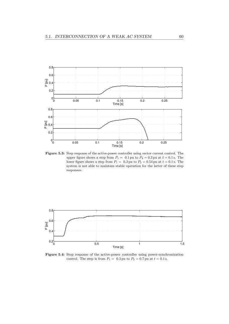
5.1. INTERCONNECTION OF A WEAK AC SYSTEM 60
0 0.05 0.1 0.15 0.2 0.250
0.2
0.4
0.6
0.8
Time [s]
P [pu]
0 0.05 0.1 0.15 0.2 0.250
0.2
0.4
0.6
0.8
Time [s]
P [pu]
Figure 5.3: Step response of the active-power controller using vector current control. Theupper figure shows a step from P1 = 0.1 pu to P2 = 0.3 pu at t = 0.1 s. Thelower figure shows a step from P1 = 0.3 pu to P2 = 0.54 pu at t = 0.1 s. Thesystem is not able to maintain stable operation for the latter of these stepresponses.
0 0.5 1 1.50.2
0.4
0.6
0.8
Time [s]
P [pu]
Figure 5.4: Step response of the active-power controller using power-synchronizationcontrol. The step is from P1 = 0.3 pu to P2 = 0.7 pu at t = 0.1 s.

5.1. INTERCONNECTION OF A WEAK AC SYSTEM 61
0 0.5 1 1.5
−1
−0.5
0
0.5
1
Time [s]
P [pu]
0 0.5 1 1.5
−1
−0.5
0
0.5
1
Time [s]
P [pu]
0 0.5 1 1.5
−1
−0.5
0
0.5
1
Time [s]
P [pu]
Figure 5.5: Active-power measurement at converter station A, C, and D, during a three-phase fault at the connecting bus of converter station A. The top, middle,and bottom figure show the power measurements of converter station A, C,and D, respectively. The fault is applied at t = 0.1 s and has a duration of100 ms.

5.1. INTERCONNECTION OF A WEAK AC SYSTEM 62
0 0.2 0.4 0.6 0.8 1 1.2 1.4 1.6 1.8 2−2
−1
0
1
2
Time [s]
i d, i q
[pu]
id
iq
0 0.2 0.4 0.6 0.8 1 1.2 1.4 1.6 1.8 2−2
−1
0
1
2
Time [s]
i d, i q
[pu]
id
iq
0 0.2 0.4 0.6 0.8 1 1.2 1.4 1.6 1.8 2−2
−1
0
1
2
Time [s]
i d, i q
[pu]
id
iq
Figure 5.6: Current measurement at converter stations A, C, and D, during a three-phasefault at the connecting bus of converter station A. The top, middle, andbottom figure show the current measurements of converter stations A, C,and D, respectively. The fault is applied at t = 0.1 s and has a duration of100 ms.

Chapter 6
Conclusions and FurtherWork
This chapter draw some conclusions from the previous chapters. Also,some suggestions to further work are made. First, chapter 3 and chapter 4are discussed, which mostly regards how the models were designed andthe controller performance comparisons of vector-current control. Second,chapter 5 is discussed, which regards the analysis of power-synchronizationcontrol.
6.1 Model Design and Controller Comparisons
Next, some conclusions regarding the graphical implementation and the Ccode implementation are drawn. Also, some suggestions to further work aremade.
6.1.1 Graphical Implementation
It is mostly without hardship to implement models graphically in PSCAD.A great advantage with PSCAD is the feature to use multiple instances.Once a control module and an AVM have been constructed, it is possibleto copy and paste these to any number of terminals, which makes it easyto construct a multi-terminal VSC-HVDC system. One drawback with thestandard PSCAD components is that it is difficult to know how they areimplemented. The PLL makes up a good example on that. If a replicaof the PLL in Simulink should be made in PSCAD, it is difficult to knowthe implementation differences. Therefore, when the model was constructedgraphically in PSCAD, the model behavior did not always make a perfectmatch to the Simulink model. A brief summary of the pros and cons withthe graphical implementation in this project follows.

6.1. MODEL DESIGN AND CONTROLLER COMPARISONS 64
Pros Cons
- Easy to construct models this way.- Multiple instances work great whenthe number of terminals increase.
- Difficult to know how stan-dard PSCAD components are imple-mented.- Hard to mimic the behavior of an-other software implementation.
6.1.2 Code Implementation
One goal for this thesis was to tailor controls in PSCAD so they replicatethe behavior of controls in Simulink. First, the model was implementedgraphically and several tests were performed on both the graphical imple-mentation and the Simulink model. However, some tests showed that it wasdifficult to mimic the exact behavior of the Simulink model. Therefore, thecontrols were also implemented using C code extracted form the Simulinkmodel. This C code was implemented in PSCAD with a nice outcome; thecontrol behavior was very similar to the Simulink model. However, theimplementation was, in comparison to the graphical implementation, ratherdifficult to achieve. Chapter 3 presents a customized interface that has to bemanually programmed for the implementation to work. Further, PSCADlacks functionality to implement multiple instances that runs on C code. Abrief summary of the pros and cons with the C code implementation in thisproject follows.
Pros Cons
- The controls can be tailored to repli-cate Simulink very well.
- Multiple instances does not work.- Necessary to manually program acustomized interface.
6.1.3 Further Work
Chapter 3 first discusses how the model can be implemented graphically. Italso discusses how the model can be implemented with C code extractedfrom the Simulink model. In order to get the C code implementation to work,chapter 3 described how to program a customized interface. This interfacelacks generality and is rather difficult to build and maintain. The modelexchange tool FMI and scripts that automatically construct the interfacewere also discussed in chapter 3. In this context, some suggestions to furtherwork follow.
- Construct a script that automatically writes the code for a customizedinterface.
- Develop something similar to FMI or extend FMI/PSCAD features forcompatibility.

6.2. POWER-SYNCHRONIZATION CONTROL 65
6.1.4 Black-Box Model Comparison
The tests with the manufacturer’s black-box model were performed with-out any knowledge about the control implementation within the black-box.Components like shunt reactors and dc link capacitors were unknown. Also,control strategies and the control tuning were unknown. In several testscenarios it seems like the generic control performs better than the black-box,which is considered to be unlikely. Probably, this is because of that themanufacturer’s black-box model might take more things into consideration(e.g., it is not modeled with an AVM). The conclusion drawn here is thatthe generic control does not perform badly in comparison to other controls.Of course, more comparisons to other control implementations and othermanufacturer’s are needed to be sure on the correctness of this conclusion.
6.2 Power-Synchronization Control
In chapter 5, power-synchronization control was investigated in a multi-terminal VSC-HVDC system. The work demonstrated how one terminalin a dc grid was connected to a very weak ac system by using power-synchronization control. In particular, the ac system was weak because of theinterconnecting lines and the conditions under which they were connected.In order to simplify the calculations, an estimation of the upper bound ofthe SCR was performed. In comparison to power-synchronization control,two step responses of the active-power controller were demonstrated usingvector current control. Particularly, the author was not able to achieve stableoperation with a power transfer of 0.54 pu using vector-current control, whilepower synchronization control reaches stable operation with a power transferof 0.7 pu.

Chapter 7
Bibliography
[1] L. Zhang, L. Harnefors, and P. Rey, “Power system reliability andtransfer capability improvement by VSC-HVDC (HVDC light),” inCigre Regional Meeting, Tallin, Estonia, 2007.
[2] N. Flourentzou, V. Agelidis, and G. Demetriades, “VSC-Based HVDCPower Transmission Systems: An Overview,” Power Electronics, IEEETransactions on, vol. 24, no. 3, pp. 592–602, 2009.
[3] L. Zhang, Modeling and Control of VSC-HVDC Links Connected toWeak AC Systems. PhD thesis, KTH, Electrical Machines and PowerElectronics, 2010. QC20100607.
[4] “IEEE Guide for Planning dc Links Terminating at ac Locations HavingLow Short-Circuit Capacities,” IEEE Std 1204-1997, pp. i–, 1997.
[5] M. Durrant, H. Werner, and K. Abbott, “Model of a VSC HVDCterminal attached to a weak ac system,” in IEEE Conference on ControlApplications, vol. 1, pp. 178–182 vol.1, 2003.
[6] L. Zhang, L. Harnefors, and H.-P. Nee, “Interconnection of Two VeryWeak ac Systems by VSC-HVDC Links Using Power-SynchronizationControl,” Power Systems, IEEE Transactions on, vol. 26, no. 1, pp. 344–355, 2011.
[7] L. Zhang and H.-P. Nee, “Multivariable feedback design of VSC-HVDCconnected to weak ac systems,” in PowerTech, 2009 IEEE Bucharest,pp. 1–8, 2009.
[8] R. Rogersten, L. Zhang, and P. Mitra, “Applying Power-SynchronizationControl in a Multi-Terminal DC System,” in IEEE PES General Meeting2014, (Washinton DC, USA), 2014.
[9] J. Arrillaga, Y. H. Liu, N. R. Watson, and N. J. Murray, Self-Commutating Converters for High Power Applications. Wiley, 2009.
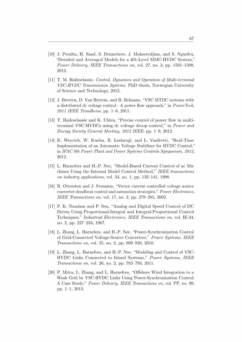
67
[10] J. Peralta, H. Saad, S. Dennetiere, J. Mahseredjian, and S. Nguefeu,“Detailed and Averaged Models for a 401-Level MMC-HVDC System,”Power Delivery, IEEE Transactions on, vol. 27, no. 3, pp. 1501–1508,2012.
[11] T. M. Haileselassie, Control, Dynamics and Operation of Multi-terminalVSC-HVDC Transmission Systems. PhD thesis, Norwegian Universityof Science and Technology, 2012.
[12] J. Beerten, D. Van Hertem, and R. Belmans, “VSC MTDC systems witha distributed dc voltage control - A power flow approach,” in PowerTech,2011 IEEE Trondheim, pp. 1–6, 2011.
[13] T. Haileselassie and K. Uhlen, “Precise control of power flow in multi-terminal VSC-HVDCs using dc voltage droop control,” in Power andEnergy Society General Meeting, 2012 IEEE, pp. 1–9, 2012.
[14] K. Weyrich, W. Kuehn, R. Leelaruji, and L. Vanfretti, “Real-TimeImplementation of an Automatic Voltage Stabilizer for HVDC Control,”in IFAC 8th Power Plant and Power Systems Controls Symposium, 2012,2012.
[15] L. Harnefors and H.-P. Nee, “Model-Based Current Control of ac Ma-chines Using the Internal Model Control Method,” IEEE transactionson industry applications, vol. 34, no. 1, pp. 133–141, 1998.
[16] R. Ottersten and J. Svensson, “Vector current controlled voltage sourceconverter-deadbeat control and saturation strategies,” Power Electronics,IEEE Transactions on, vol. 17, no. 2, pp. 279–285, 2002.
[17] P. K. Nandam and P. Sen, “Analog and Digital Speed Control of DCDrives Using Proportional-Integral and Integral-Proportional ControlTechniques,” Industrial Electronics, IEEE Transactions on, vol. IE-34,no. 2, pp. 227–233, 1987.
[18] L. Zhang, L. Harnefors, and H.-P. Nee, “Power-Synchronization Controlof Grid-Connected Voltage-Source Converters,” Power Systems, IEEETransactions on, vol. 25, no. 2, pp. 809–820, 2010.
[19] L. Zhang, L. Harnefors, and H.-P. Nee, “Modeling and Control of VSC-HVDC Links Connected to Island Systems,” Power Systems, IEEETransactions on, vol. 26, no. 2, pp. 783–793, 2011.
[20] P. Mitra, L. Zhang, and L. Harnefors, “Offshore Wind Integration to aWeak Grid by VSC-HVDC Links Using Power-Synchronization Control:A Case Study,” Power Delivery, IEEE Transactions on, vol. PP, no. 99,pp. 1–1, 2013.

68
[21] L. Zhang, H.-P. Nee, and L. Harnefors, “Analysis of Stability Limitationsof a VSC-HVDC Link Using Power-Synchronization Control,” PowerSystems, IEEE Transactions on, vol. 26, no. 3, pp. 1326–1337, 2011.
[22] M. Faruque, Y. Zhang, and V. Dinavahi, “Detailed modelingof CIGRE HVDC benchmark system using PSCAD/EMTDC andPSB/SIMULINK,” Power Delivery, IEEE Transactions on, vol. 21,pp. 378–387, Jan 2006.
[23] R. Rogersten, H. Xu, N. Ozay, U. Topcu, and R. Murray, “Synthesisand Validation of Control Software For A Vehicular Electric Power Dis-tribution Testbed,” accepted by AIAA Journal of Aerospace InformationSystems, 2014.
[24] “FMI.” www.fmi-standard.org/. Retrieved 17 February 2014.
[25] A. B. Bondi, “Characteristics of Scalability and Their Impact on Perfor-mance,” in Proceedings of the 2Nd International Workshop on Softwareand Performance, WOSP ’00, (New York, NY, USA), pp. 195–203,ACM, 2000.

Appendix A
Voltage Plots During Faults

70
0 0.1 0.2 0.3 0.4 0.5 0.6
−1.5
−1
−0.5
0
0.5
1
1.5
Time [s]
Voltage [pu]
Figure A.1: Instantanous voltage mesurement during a three-phase fault at t = 0.2 s with10% remaining voltage. This voltage plot is from Simulink. The voltageplots from PSCAD are very similar and therefore not shown here.
0 0.1 0.2 0.3 0.4 0.5 0.6
−1.5
−1
−0.5
0
0.5
1
1.5
Time [s]
Voltage [pu]
Figure A.2: Instantanous voltage mesurement during a three-phase fault at t = 0.2 s with30% remaining voltage. This voltage plot is from Simulink. The voltageplots from PSCAD are very similar and therefore not shown here.

71
0 0.1 0.2 0.3 0.4 0.5 0.6
−1.5
−1
−0.5
0
0.5
1
1.5
Time [s]
Voltage [pu]
Figure A.3: Instantanous voltage mesurement during a three-phase fault at t = 0.2 s with70% remaining voltage. This voltage plot is from Simulink. The voltageplots from PSCAD are very similar and therefore not shown here.
0 0.1 0.2 0.3 0.4 0.5 0.6
−1.5
−1
−0.5
0
0.5
1
1.5
Time [s]
Voltage [pu]
Figure A.4: Instantanous voltage mesurement during a single-phase fault at t = 0.2 swith 10% remaining voltage. This voltage plot is from Simulink. The voltageplots from PSCAD are very similar and therefore not shown here.

72
0 0.1 0.2 0.3 0.4 0.5 0.6
−1.5
−1
−0.5
0
0.5
1
1.5
Time [s]
Voltage [pu]
Figure A.5: Instantanous voltage mesurement during a single-phase fault at t = 0.2 swith 30% remaining voltage. This voltage plot is from Simulink. The voltageplots from PSCAD are very similar and therefore not shown here.
0 0.1 0.2 0.3 0.4 0.5 0.6
−1.5
−1
−0.5
0
0.5
1
1.5
Time [s]
Voltage [pu]
Figure A.6: Instantanous voltage mesurement during a single-phase fault at t = 0.2 swith 70% remaining voltage. This voltage plot is from Simulink. The voltageplots from PSCAD are very similar and therefore not shown here.

Appendix B
Graphical Implementation
B.1 Step of the Active- and Reactive-Power Con-troller

B.1. STEP OF THE ACTIVE- AND REACTIVE-POWERCONTROLLER 74
1.5 2 2.5 3−0.2
−0.1
0
0.1
0.2
0.3
0.4
0.5
Time [s]
P [pu]
SIMULINKPSCAD
1.5 2 2.5 3−0.2
−0.1
0
0.1
0.2
0.3
0.4
0.5
Time [s]
Q [pu]
SIMULINKPSCAD
Figure B.1: Active power step change by 30% at t = 2 s. The upper figure illustrates thechange in active power and the lower figure illustrates the change in reactivepower due to that the system is coupled.

B.1. STEP OF THE ACTIVE- AND REACTIVE-POWERCONTROLLER 75
1.5 2 2.5 3−0.2
−0.1
0
0.1
0.2
0.3
0.4
0.5
Time [s]
i dref [
pu]
SIMULINKPSCAD
1.5 2 2.5 3−0.2
−0.1
0
0.1
0.2
0.3
0.4
0.5
Time [s]
i qref [
pu]
SIMULINKPSCAD
1.5 2 2.5 3−0.2
−0.1
0
0.1
0.2
0.3
0.4
0.5
Time [s]
|idq| [p
u]
SIMULINKPSCAD
Figure B.2: The two upper figures show the change of the reference currents irefd andirefq during the active power step change by 30% at t = 2 s. The lowerfigure illustrates the changes in the current |idq| during the active powerstep change by 30% at t = 2 s.
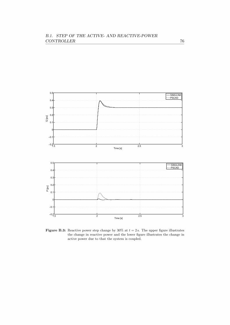
B.1. STEP OF THE ACTIVE- AND REACTIVE-POWERCONTROLLER 76
1.5 2 2.5 3−0.2
−0.1
0
0.1
0.2
0.3
0.4
0.5
Time [s]
Q [pu]
SIMULINKPSCAD
1.5 2 2.5 3−0.2
−0.1
0
0.1
0.2
0.3
0.4
0.5
Time [s]
P [pu]
SIMULINKPSCAD
Figure B.3: Reactive power step change by 30% at t = 2 s. The upper figure illustratesthe change in reactive power and the lower figure illustrates the change inactive power due to that the system is coupled.

B.1. STEP OF THE ACTIVE- AND REACTIVE-POWERCONTROLLER 77
1.5 2 2.5 3−0.5
−0.4
−0.3
−0.2
−0.1
0
0.1
0.2
0.3
0.4
0.5
Time [s]
i dref [
pu]
SIMULINKPSCAD
1.5 2 2.5 3−0.5
−0.4
−0.3
−0.2
−0.1
0
0.1
0.2
0.3
0.4
0.5
Time [s]
i qref [
pu]
SIMULINKPSCAD
1.5 2 2.5 3−0.5
−0.4
−0.3
−0.2
−0.1
0
0.1
0.2
0.3
0.4
0.5
Time [s]
|idq| [p
u]
SIMULINKPSCAD
Figure B.4: The two upper figures show the change of the reference currents irefd andirefq during the reactive power step change by 30% at t = 2 s. The lowerfigure illustrates the changes in the current |idq| during the reactive powerstep change by 30% at t = 2 s.

B.2. THREE-PHASE FAULTS (FAULT SCENARIOS 3 TO 5) 78
B.2 Three-Phase Faults (Fault Scenarios 3 to 5)

B.2. THREE-PHASE FAULTS (FAULT SCENARIOS 3 TO 5) 79
1.5 2 2.5 3−1
−0.5
0
0.5
1
1.5
Time [s]
P [pu]
SIMULINKPSCAD
1.5 2 2.5 3−1
−0.5
0
0.5
1
1.5
Time [s]
Q [pu]
SIMULINKPSCAD
Figure B.5: Three-phase fault at t = 2 s with 10% remaining voltage. The upper figureillustrates the change in active power and the lower figure illustrates thechange in reactive power due to that the system is coupled.

B.2. THREE-PHASE FAULTS (FAULT SCENARIOS 3 TO 5) 80
1.5 2 2.5 3−1
−0.5
0
0.5
1
1.5
Time [s]
i dref [
pu]
SIMULINKPSCAD
1.5 2 2.5 3−1
−0.5
0
0.5
1
1.5
Time [s]
i qref [
pu]
SIMULINKPSCAD
1.5 2 2.5 3−1
−0.5
0
0.5
1
1.5
Time [s]
|idq| [p
u]
SIMULINKPSCAD
Figure B.6: Three-phase fault at t = 2 s with 10% remaining voltage. The two upperfigures show the change of the reference currents irefd and irefq . The lowerfigure illustrates the changes in the current |idq|.

B.2. THREE-PHASE FAULTS (FAULT SCENARIOS 3 TO 5) 81
1.5 2 2.5 3−1
−0.5
0
0.5
1
1.5
Time [s]
P [pu]
SIMULINKPSCAD
1.5 2 2.5 3−1
−0.5
0
0.5
1
1.5
Time [s]
Q [pu]
SIMULINKPSCAD
Figure B.7: Three-phase fault at t = 2 s with 30% remaining voltage. The upper figureillustrates the change in active power and the lower figure illustrates thechange in reactive power due to that the system is coupled.

B.2. THREE-PHASE FAULTS (FAULT SCENARIOS 3 TO 5) 82
1.5 2 2.5 3−1
−0.5
0
0.5
1
1.5
Time [s]
i dref [
pu]
SIMULINKPSCAD
1.5 2 2.5 3−1
−0.5
0
0.5
1
1.5
Time [s]
i qref [
pu]
SIMULINKPSCAD
1.5 2 2.5 3−1
−0.5
0
0.5
1
1.5
Time [s]
|idq| [p
u]
SIMULINKPSCAD
Figure B.8: Three-phase fault at t = 2 s with 30% remaining voltage. The two upperfigures show the change of the reference currents irefd and irefq . The lowerfigure illustrates the changes in the current |idq|.

B.2. THREE-PHASE FAULTS (FAULT SCENARIOS 3 TO 5) 83
1.5 2 2.5 3−1
−0.5
0
0.5
1
1.5
Time [s]
P [pu]
SIMULINKPSCAD
1.5 2 2.5 3−1
−0.5
0
0.5
1
1.5
Time [s]
Q [pu]
SIMULINKPSCAD
Figure B.9: Three-phase fault at t = 2 s with 70% remaining voltage. The upper figureillustrates the change in active power and the lower figure illustrates thechange in reactive power due to that the system is coupled.

B.2. THREE-PHASE FAULTS (FAULT SCENARIOS 3 TO 5) 84
1.5 2 2.5 3−1
−0.5
0
0.5
1
1.5
Time [s]
i dref [
pu]
SIMULINKPSCAD
1.5 2 2.5 3−1
−0.5
0
0.5
1
1.5
Time [s]
i qref [
pu]
SIMULINKPSCAD
1.5 2 2.5 3−1
−0.5
0
0.5
1
1.5
Time [s]
|idq| [p
u]
SIMULINKPSCAD
Figure B.10: Three-phase fault at t = 2 s with 70% remaining voltage. The two upperfigures show the change of the reference currents irefd and irefq . The lowerfigure illustrates the changes in the current |idq|.

B.3. SINGLE-PHASE FAULTS (FAULT SCENARIOS 6 TO 8) 85
B.3 Single-Phase Faults (Fault Scenarios 6 to 8)

B.3. SINGLE-PHASE FAULTS (FAULT SCENARIOS 6 TO 8) 86
1.5 2 2.5 3−1
−0.5
0
0.5
1
1.5
Time [s]
P [pu]
SIMULINKPSCAD
1.5 2 2.5 3−1
−0.5
0
0.5
1
1.5
Time [s]
Q [pu]
SIMULINKPSCAD
Figure B.11: Single-phase fault at t = 2 s with 10% remaining voltage. The upper figureillustrates the change in active power and the lower figure illustrates thechange in reactive power due to that the system is coupled.

B.3. SINGLE-PHASE FAULTS (FAULT SCENARIOS 6 TO 8) 87
1.5 2 2.5 3−1
−0.5
0
0.5
1
1.5
Time [s]
i dref [
pu]
SIMULINKPSCAD
1.5 2 2.5 3−1
−0.5
0
0.5
1
1.5
Time [s]
i qref [
pu]
SIMULINKPSCAD
1.5 2 2.5 3−1
−0.5
0
0.5
1
1.5
Time [s]
|idq| [p
u]
SIMULINKPSCAD
Figure B.12: Single-phase fault at t = 2 s with 10% remaining voltage. The two upperfigures show the change of the reference currents irefd and irefq . The lowerfigure illustrates the changes in the current |idq|.

B.3. SINGLE-PHASE FAULTS (FAULT SCENARIOS 6 TO 8) 88
1.5 2 2.5 3−1
−0.5
0
0.5
1
1.5
Time [s]
P [pu]
SIMULINKPSCAD
1.5 2 2.5 3−1
−0.5
0
0.5
1
1.5
Time [s]
Q [pu]
SIMULINKPSCAD
Figure B.13: Single-phase fault at t = 2 s with 30% remaining voltage. The upper figureillustrates the change in active power and the lower figure illustrates thechange in reactive power due to that the system is coupled.

B.3. SINGLE-PHASE FAULTS (FAULT SCENARIOS 6 TO 8) 89
1.5 2 2.5 3−1
−0.5
0
0.5
1
1.5
Time [s]
i dref [
pu]
SIMULINKPSCAD
1.5 2 2.5 3−1
−0.5
0
0.5
1
1.5
Time [s]
i qref [
pu]
SIMULINKPSCAD
1.5 2 2.5 3−1
−0.5
0
0.5
1
1.5
Time [s]
|idq| [p
u]
SIMULINKPSCAD
Figure B.14: Single-phase fault at t = 2 s with 30% remaining voltage. The two upperfigures show the change of the reference currents irefd and irefq . The lowerfigure illustrates the changes in the current |idq|.

B.3. SINGLE-PHASE FAULTS (FAULT SCENARIOS 6 TO 8) 90
1.5 2 2.5 3−1
−0.5
0
0.5
1
1.5
Time [s]
P [pu]
SIMULINKPSCAD
1.5 2 2.5 3−1
−0.5
0
0.5
1
1.5
Time [s]
Q [pu]
SIMULINKPSCAD
Figure B.15: Single-phase fault at t = 2 s with 70% remaining voltage. The upper figureillustrates the change in active power and the lower figure illustrates thechange in reactive power due to that the system is coupled.

B.3. SINGLE-PHASE FAULTS (FAULT SCENARIOS 6 TO 8) 91
1.5 2 2.5 3−1
−0.5
0
0.5
1
1.5
Time [s]
i dref [
pu]
SIMULINKPSCAD
1.5 2 2.5 3−1
−0.5
0
0.5
1
1.5
Time [s]
i qref [
pu]
SIMULINKPSCAD
1.5 2 2.5 3−1
−0.5
0
0.5
1
1.5
Time [s]
|idq| [p
u]
SIMULINKPSCAD
Figure B.16: Single-phase fault at t = 2 s with 70% remaining voltage. The two upperfigures show the change of the reference currents irefd and irefq . The lowerfigure illustrates the changes in the current |idq|.

Appendix C
Code Implementation
C.1 Step of the Active- and Reactive-Power Con-troller

C.1. STEP OF THE ACTIVE- AND REACTIVE-POWERCONTROLLER 93
3.5 4 4.5 5−0.2
−0.1
0
0.1
0.2
0.3
0.4
0.5
Time [s]
P [pu]
SIMULINKPSCAD
3.5 4 4.5 5−0.2
−0.1
0
0.1
0.2
0.3
0.4
0.5
Time [s]
Q [pu]
SIMULINKPSCAD
Figure C.1: Active power step change by 30% at t = 4 s. The upper figure illustrates thechange in active power and the lower figure illustrates the change in reactivepower due to that the system is coupled.

C.1. STEP OF THE ACTIVE- AND REACTIVE-POWERCONTROLLER 94
3.5 4 4.5 5−0.2
−0.1
0
0.1
0.2
0.3
0.4
0.5
Time [s]
i dref [
pu]
SIMULINKPSCAD
3.5 4 4.5 5−0.2
−0.1
0
0.1
0.2
0.3
0.4
0.5
Time [s]
i qref [
pu]
SIMULINKPSCAD
3.5 4 4.5 5−0.2
−0.1
0
0.1
0.2
0.3
0.4
0.5
Time [s]
|idq| [p
u]
SIMULINKPSCAD
Figure C.2: The two upper figures show the change of the reference currents irefd andirefq during the active power step change by 30% at t = 4 s. The lowerfigure illustrates the changes in the current |idq| during the active powerstep change by 30% at t = 4 s.

C.1. STEP OF THE ACTIVE- AND REACTIVE-POWERCONTROLLER 95
3.5 4 4.5 5−0.2
−0.1
0
0.1
0.2
0.3
0.4
0.5
Time [s]
Q [pu]
SIMULINKPSCAD
3.5 4 4.5 5−0.2
−0.1
0
0.1
0.2
0.3
0.4
0.5
Time [s]
P [pu]
SIMULINKPSCAD
Figure C.3: Reactive power step change by 30% at t = 4 s. The upper figure illustratesthe change in reactive power and the lower figure illustrates the change inactive power due to that the system is coupled.

C.1. STEP OF THE ACTIVE- AND REACTIVE-POWERCONTROLLER 96
3.5 4 4.5 5−0.5
−0.4
−0.3
−0.2
−0.1
0
0.1
0.2
0.3
0.4
0.5
Time [s]
i dref [
pu]
SIMULINKPSCAD
3.5 4 4.5 5−0.5
−0.4
−0.3
−0.2
−0.1
0
0.1
0.2
0.3
0.4
0.5
Time [s]
i qref [
pu]
SIMULINKPSCAD
3.5 4 4.5 5−0.5
−0.4
−0.3
−0.2
−0.1
0
0.1
0.2
0.3
0.4
0.5
Time [s]
|idq| [p
u]
SIMULINKPSCAD
Figure C.4: The two upper figures show the change of the reference currents irefd andirefq during the reactive power step change by 30% at t = 4 s. The lowerfigure illustrates the changes in the current |idq| during the reactive powerstep change by 30% at t = 4 s.

C.2. THREE-PHASE FAULTS (FAULT SCENARIOS 3 TO 5) 97
C.2 Three-Phase Faults (Fault Scenarios 3 to 5)

C.2. THREE-PHASE FAULTS (FAULT SCENARIOS 3 TO 5) 98
3.5 4 4.5 5−1
−0.5
0
0.5
1
1.5
Time [s]
P [pu]
SIMULINKPSCAD
3.5 4 4.5 5−1
−0.5
0
0.5
1
1.5
Time [s]
Q [pu]
SIMULINKPSCAD
Figure C.5: Three-phase fault at t = 4 s with 10% remaining voltage. The upper figureillustrates the change in active power and the lower figure illustrates thechange in reactive power due to that the system is coupled.

C.2. THREE-PHASE FAULTS (FAULT SCENARIOS 3 TO 5) 99
3.5 4 4.5 5−1
−0.5
0
0.5
1
1.5
Time [s]
i dref [
pu]
SIMULINKPSCAD
3.5 4 4.5 5−1
−0.5
0
0.5
1
1.5
Time [s]
i qref [
pu]
SIMULINKPSCAD
3.5 4 4.5 5−1
−0.5
0
0.5
1
1.5
Time [s]
|idq| [p
u]
SIMULINKPSCAD
Figure C.6: Three-phase fault at t = 4 s with 10% remaining voltage. The two upperfigures show the change of the reference currents irefd and irefq . The lowerfigure illustrates the changes in the current |idq|.

C.2. THREE-PHASE FAULTS (FAULT SCENARIOS 3 TO 5) 100
3.5 4 4.5 5−1
−0.5
0
0.5
1
1.5
Time [s]
P [pu]
SIMULINKPSCAD
3.5 4 4.5 5−1
−0.5
0
0.5
1
1.5
Time [s]
Q [pu]
SIMULINKPSCAD
Figure C.7: Three-phase fault at t = 4 s with 30% remaining voltage. The upper figureillustrates the change in active power and the lower figure illustrates thechange in reactive power due to that the system is coupled.
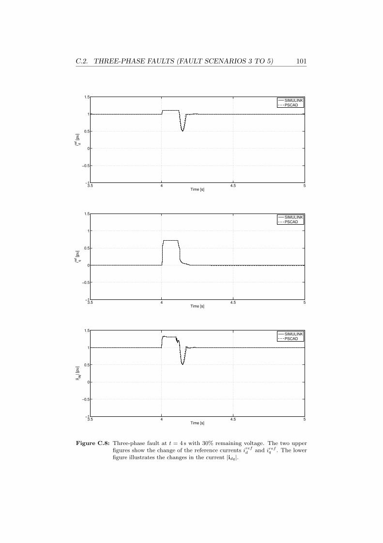
C.2. THREE-PHASE FAULTS (FAULT SCENARIOS 3 TO 5) 101
3.5 4 4.5 5−1
−0.5
0
0.5
1
1.5
Time [s]
i dref [
pu]
SIMULINKPSCAD
3.5 4 4.5 5−1
−0.5
0
0.5
1
1.5
Time [s]
i qref [
pu]
SIMULINKPSCAD
3.5 4 4.5 5−1
−0.5
0
0.5
1
1.5
Time [s]
|idq| [p
u]
SIMULINKPSCAD
Figure C.8: Three-phase fault at t = 4 s with 30% remaining voltage. The two upperfigures show the change of the reference currents irefd and irefq . The lowerfigure illustrates the changes in the current |idq|.
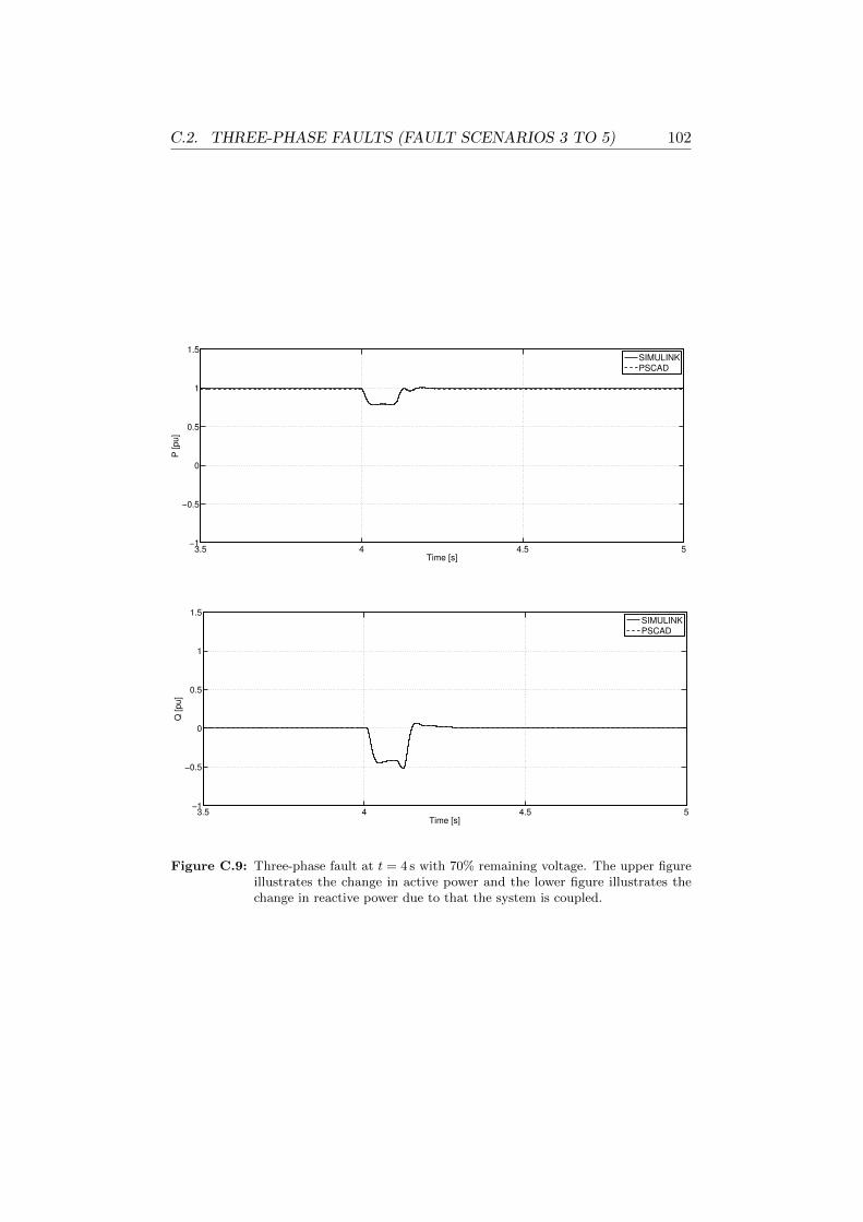
C.2. THREE-PHASE FAULTS (FAULT SCENARIOS 3 TO 5) 102
3.5 4 4.5 5−1
−0.5
0
0.5
1
1.5
Time [s]
P [pu]
SIMULINKPSCAD
3.5 4 4.5 5−1
−0.5
0
0.5
1
1.5
Time [s]
Q [pu]
SIMULINKPSCAD
Figure C.9: Three-phase fault at t = 4 s with 70% remaining voltage. The upper figureillustrates the change in active power and the lower figure illustrates thechange in reactive power due to that the system is coupled.

C.2. THREE-PHASE FAULTS (FAULT SCENARIOS 3 TO 5) 103
3.5 4 4.5 5−1
−0.5
0
0.5
1
1.5
Time [s]
i dref [
pu]
SIMULINKPSCAD
3.5 4 4.5 5−1
−0.5
0
0.5
1
1.5
Time [s]
i qref [
pu]
SIMULINKPSCAD
3.5 4 4.5 5−1
−0.5
0
0.5
1
1.5
Time [s]
|idq| [p
u]
SIMULINKPSCAD
Figure C.10: Three-phase fault at t = 4 s with 70% remaining voltage. The two upperfigures show the change of the reference currents irefd and irefq . The lowerfigure illustrates the changes in the current |idq|.

C.3. SINGLE-PHASE FAULTS (FAULT SCENARIOS 6 TO 8) 104
C.3 Single-Phase Faults (Fault Scenarios 6 to 8)

C.3. SINGLE-PHASE FAULTS (FAULT SCENARIOS 6 TO 8) 105
3.5 4 4.5 5−1
−0.5
0
0.5
1
1.5
Time [s]
P [pu]
SIMULINKPSCAD
3.5 4 4.5 5−1
−0.5
0
0.5
1
1.5
Time [s]
Q [pu]
SIMULINKPSCAD
Figure C.11: Single-phase fault at t = 4 s with 10% remaining voltage. The upper figureillustrates the change in active power and the lower figure illustrates thechange in reactive power due to that the system is coupled.

C.3. SINGLE-PHASE FAULTS (FAULT SCENARIOS 6 TO 8) 106
3.5 4 4.5 5−1
−0.5
0
0.5
1
1.5
Time [s]
i dref [
pu]
SIMULINKPSCAD
3.5 4 4.5 5−1
−0.5
0
0.5
1
1.5
Time [s]
i qref [
pu]
SIMULINKPSCAD
3.5 4 4.5 5−1
−0.5
0
0.5
1
1.5
Time [s]
|idq| [p
u]
SIMULINKPSCAD
Figure C.12: Single-phase fault at t = 4 s with 10% remaining voltage. The two upperfigures show the change of the reference currents irefd and irefq . The lowerfigure illustrates the changes in the current |idq|.

C.3. SINGLE-PHASE FAULTS (FAULT SCENARIOS 6 TO 8) 107
3.5 4 4.5 5−1
−0.5
0
0.5
1
1.5
Time [s]
P [pu]
SIMULINKPSCAD
3.5 4 4.5 5−1
−0.5
0
0.5
1
1.5
Time [s]
Q [pu]
SIMULINKPSCAD
Figure C.13: Single-phase fault at t = 4 s with 30% remaining voltage. The upper figureillustrates the change in active power and the lower figure illustrates thechange in reactive power due to that the system is coupled.

C.3. SINGLE-PHASE FAULTS (FAULT SCENARIOS 6 TO 8) 108
3.5 4 4.5 5−1
−0.5
0
0.5
1
1.5
Time [s]
i dref [
pu]
SIMULINKPSCAD
3.5 4 4.5 5−1
−0.5
0
0.5
1
1.5
Time [s]
i qref [
pu]
SIMULINKPSCAD
3.5 4 4.5 5−1
−0.5
0
0.5
1
1.5
Time [s]
|idq| [p
u]
SIMULINKPSCAD
Figure C.14: Single-phase fault at t = 4 s with 30% remaining voltage. The two upperfigures show the change of the reference currents irefd and irefq . The lowerfigure illustrates the changes in the current |idq|.

C.3. SINGLE-PHASE FAULTS (FAULT SCENARIOS 6 TO 8) 109
3.5 4 4.5 5−1
−0.5
0
0.5
1
1.5
Time [s]
P [pu]
SIMULINKPSCAD
3.5 4 4.5 5−1
−0.5
0
0.5
1
1.5
Time [s]
Q [pu]
SIMULINKPSCAD
Figure C.15: Single-phase fault at t = 4 s with 70% remaining voltage. The upper figureillustrates the change in active power and the lower figure illustrates thechange in reactive power due to that the system is coupled.

C.3. SINGLE-PHASE FAULTS (FAULT SCENARIOS 6 TO 8) 110
3.5 4 4.5 5−1
−0.5
0
0.5
1
1.5
Time [s]
i dref [
pu]
SIMULINKPSCAD
3.5 4 4.5 5−1
−0.5
0
0.5
1
1.5
Time [s]
i qref [
pu]
SIMULINKPSCAD
3.5 4 4.5 5−1
−0.5
0
0.5
1
1.5
Time [s]
|idq| [p
u]
SIMULINKPSCAD
Figure C.16: Single-phase fault at t = 4 s with 70% remaining voltage. The two upperfigures show the change of the reference currents irefd and irefq . The lowerfigure illustrates the changes in the current |idq|.

Appendix D
Black-Box ModelComparisons
D.1 Step of the Active- and Reactive-Power Con-troller

D.1. STEP OF THE ACTIVE- AND REACTIVE-POWERCONTROLLER 112
0 0.2 0.4 0.6 0.8 1 1.2 1.4 1.6 1.8 2−0.2
−0.1
0
0.1
0.2
0.3
0.4
0.5
Time [s]
P [pu]
Manufacturer’s black−box modelGeneric control
0 0.2 0.4 0.6 0.8 1 1.2 1.4 1.6 1.8 2−0.2
−0.1
0
0.1
0.2
0.3
0.4
0.5
Time [s]
Q [pu]
Manufacturer’s black−box modelGeneric control
Figure D.1: Active power step change by 30% at t = 0.2 s. The upper figure illustratesthe change in active power and the lower figure illustrates the change inreactive power due to that the system is coupled.

D.1. STEP OF THE ACTIVE- AND REACTIVE-POWERCONTROLLER 113
0 0.2 0.4 0.6 0.8 1 1.2 1.4 1.6 1.8 2−0.2
−0.1
0
0.1
0.2
0.3
0.4
0.5
Time [s]
Q [pu]
Manufacturer’s black−box modelGeneric control
0 0.2 0.4 0.6 0.8 1 1.2 1.4 1.6 1.8 2−0.2
−0.1
0
0.1
0.2
0.3
0.4
0.5
Time [s]
P [pu]
Manufacturer’s black−box modelGeneric control
Figure D.2: Reactive power step change by 30% at t = 0.2 s. The upper figure illustratesthe change in reactive power and the lower figure illustrates the change inactive power due to that the system is coupled.

D.2. THREE-PHASE FAULTS AT RECTIFIER SIDE (FAULTSCENARIOS 3 TO 5) 114
D.2 Three-Phase Faults at Rectifier Side (FaultScenarios 3 to 5)

D.2. THREE-PHASE FAULTS AT RECTIFIER SIDE (FAULTSCENARIOS 3 TO 5) 115
0 0.2 0.4 0.6 0.8 1 1.2 1.4 1.6 1.8 2−1
−0.5
0
0.5
1
1.5
Time [s]
P [
pu
]
Manufacturer’s black−box modelGeneric control
0 0.2 0.4 0.6 0.8 1 1.2 1.4 1.6 1.8 2−1
−0.5
0
0.5
1
1.5
Time [s]
Q [pu]
Manufacturer’s black−box modelGeneric control
Figure D.3: Three-phase fault at t = 0.2 s with 10% remaining voltage. The fault isapplied on the rectifier side. The upper figure illustrates the change in activepower and the lower figure illustrates the change in reactive power due tothat the system is coupled.

D.2. THREE-PHASE FAULTS AT RECTIFIER SIDE (FAULTSCENARIOS 3 TO 5) 116
0 0.2 0.4 0.6 0.8 1 1.2 1.4 1.6 1.8 2−1
−0.5
0
0.5
1
1.5
Time [s]
P [
pu
]
Manufacturer’s black−box modelGeneric control
0 0.2 0.4 0.6 0.8 1 1.2 1.4 1.6 1.8 2−1
−0.5
0
0.5
1
1.5
Time [s]
Q [pu]
Manufacturer’s black−box modelGeneric control
Figure D.4: Three-phase fault at t = 0.2 s with 30% remaining voltage. The fault isapplied on the rectifier side. The upper figure illustrates the change in activepower and the lower figure illustrates the change in reactive power due tothat the system is coupled.
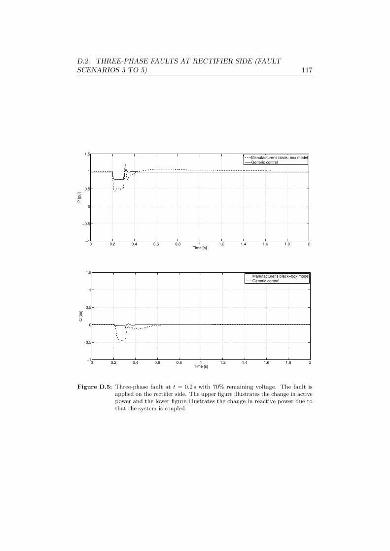
D.2. THREE-PHASE FAULTS AT RECTIFIER SIDE (FAULTSCENARIOS 3 TO 5) 117
0 0.2 0.4 0.6 0.8 1 1.2 1.4 1.6 1.8 2−1
−0.5
0
0.5
1
1.5
Time [s]
P [
pu
]
Manufacturer’s black−box modelGeneric control
0 0.2 0.4 0.6 0.8 1 1.2 1.4 1.6 1.8 2−1
−0.5
0
0.5
1
1.5
Time [s]
Q [pu]
Manufacturer’s black−box modelGeneric control
Figure D.5: Three-phase fault at t = 0.2 s with 70% remaining voltage. The fault isapplied on the rectifier side. The upper figure illustrates the change in activepower and the lower figure illustrates the change in reactive power due tothat the system is coupled.

D.3. SINGLE-PHASE FAULTS AT RECTIFIER SIDE (FAULTSCENARIOS 6 TO 8) 118
D.3 Single-Phase Faults at Rectifier Side (FaultScenarios 6 to 8)

D.3. SINGLE-PHASE FAULTS AT RECTIFIER SIDE (FAULTSCENARIOS 6 TO 8) 119
0 0.2 0.4 0.6 0.8 1 1.2 1.4 1.6 1.8 2−1
−0.5
0
0.5
1
1.5
2
Time [s]
P [
pu
]
Manufacturer’s black−box modelGeneric control
0 0.2 0.4 0.6 0.8 1 1.2 1.4 1.6 1.8 2−1
−0.5
0
0.5
1
1.5
2
Time [s]
Q [pu]
Manufacturer’s black−box modelGeneric control
Figure D.6: Single-phase fault at t = 0.2 s with 10% remaining voltage. The fault isapplied on the rectifier side. The upper figure illustrates the change in activepower and the lower figure illustrates the change in reactive power due tothat the system is coupled.

D.3. SINGLE-PHASE FAULTS AT RECTIFIER SIDE (FAULTSCENARIOS 6 TO 8) 120
0 0.2 0.4 0.6 0.8 1 1.2 1.4 1.6 1.8 2−1
−0.5
0
0.5
1
1.5
Time [s]
P [
pu
]
Manufacturer’s black−box modelGeneric control
0 0.2 0.4 0.6 0.8 1 1.2 1.4 1.6 1.8 2−1
−0.5
0
0.5
1
1.5
Time [s]
Q [pu]
Manufacturer’s black−box modelGeneric control
Figure D.7: Single-phase fault at t = 0.2 s with 30% remaining voltage. The fault isapplied on the rectifier side. The upper figure illustrates the change in activepower and the lower figure illustrates the change in reactive power due tothat the system is coupled.

D.3. SINGLE-PHASE FAULTS AT RECTIFIER SIDE (FAULTSCENARIOS 6 TO 8) 121
0 0.2 0.4 0.6 0.8 1 1.2 1.4 1.6 1.8 2−1
−0.5
0
0.5
1
1.5
Time [s]
P [
pu
]
Manufacturer’s black−box modelGeneric control
0 0.2 0.4 0.6 0.8 1 1.2 1.4 1.6 1.8 2−1
−0.5
0
0.5
1
1.5
Time [s]
Q [pu]
Manufacturer’s black−box modelGeneric control
Figure D.8: Single-phase fault at t = 0.2 s with 70% remaining voltage. The fault isapplied on the rectifier side. The upper figure illustrates the change in activepower and the lower figure illustrates the change in reactive power due tothat the system is coupled.

D.4. THREE-PHASE FAULTS AT INVERTER SIDE (FAULTSCENARIOS 3 TO 5) 122
D.4 Three-Phase Faults at Inverter Side (FaultScenarios 3 to 5)
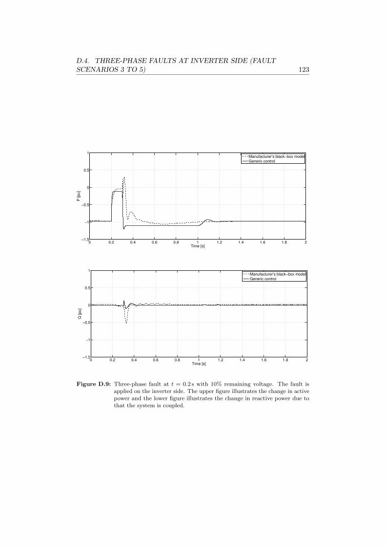
D.4. THREE-PHASE FAULTS AT INVERTER SIDE (FAULTSCENARIOS 3 TO 5) 123
0 0.2 0.4 0.6 0.8 1 1.2 1.4 1.6 1.8 2−1.5
−1
−0.5
0
0.5
1
Time [s]
P [
pu
]
Manufacturer’s black−box modelGeneric control
0 0.2 0.4 0.6 0.8 1 1.2 1.4 1.6 1.8 2−1.5
−1
−0.5
0
0.5
1
Time [s]
Q [pu]
Manufacturer’s black−box modelGeneric control
Figure D.9: Three-phase fault at t = 0.2 s with 10% remaining voltage. The fault isapplied on the inverter side. The upper figure illustrates the change in activepower and the lower figure illustrates the change in reactive power due tothat the system is coupled.
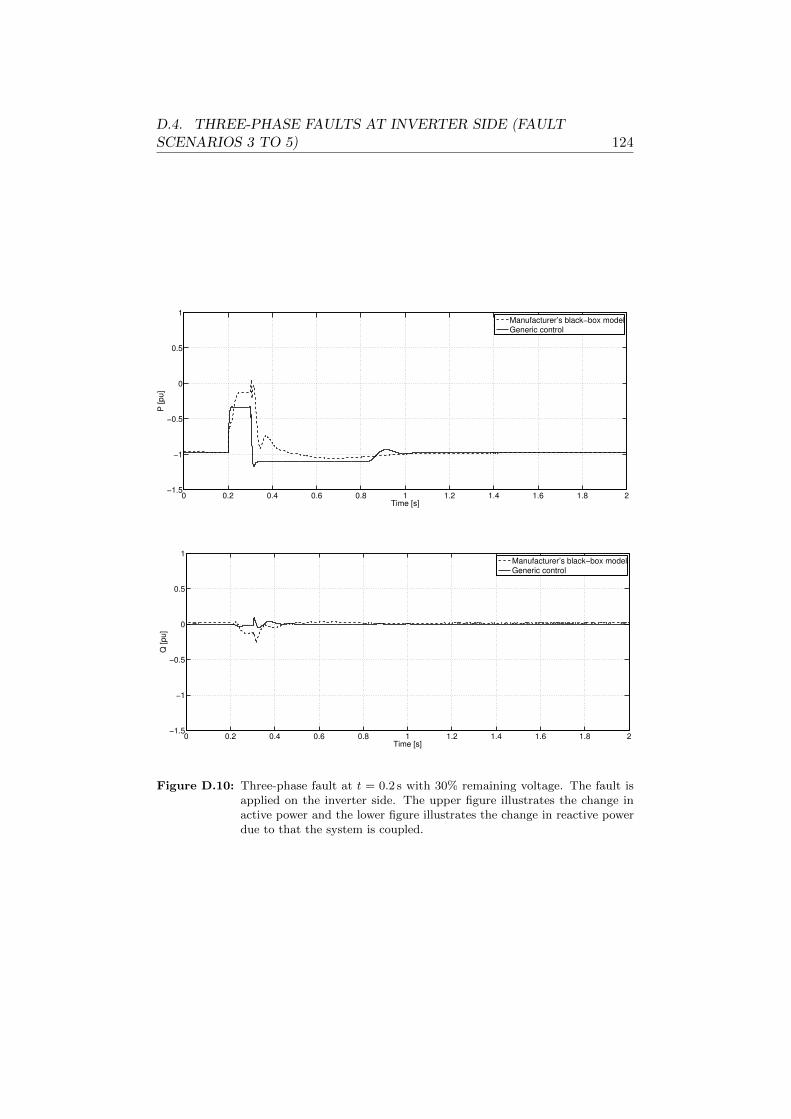
D.4. THREE-PHASE FAULTS AT INVERTER SIDE (FAULTSCENARIOS 3 TO 5) 124
0 0.2 0.4 0.6 0.8 1 1.2 1.4 1.6 1.8 2−1.5
−1
−0.5
0
0.5
1
Time [s]
P [
pu
]
Manufacturer’s black−box modelGeneric control
0 0.2 0.4 0.6 0.8 1 1.2 1.4 1.6 1.8 2−1.5
−1
−0.5
0
0.5
1
Time [s]
Q [pu]
Manufacturer’s black−box modelGeneric control
Figure D.10: Three-phase fault at t = 0.2 s with 30% remaining voltage. The fault isapplied on the inverter side. The upper figure illustrates the change inactive power and the lower figure illustrates the change in reactive powerdue to that the system is coupled.

D.4. THREE-PHASE FAULTS AT INVERTER SIDE (FAULTSCENARIOS 3 TO 5) 125
0 0.2 0.4 0.6 0.8 1 1.2 1.4 1.6 1.8 2−1.5
−1
−0.5
0
0.5
1
Time [s]
P [
pu
]
Manufacturer’s black−box modelGeneric control
0 0.2 0.4 0.6 0.8 1 1.2 1.4 1.6 1.8 2−1.5
−1
−0.5
0
0.5
1
Time [s]
Q [pu]
Manufacturer’s black−box modelGeneric control
Figure D.11: Three-phase fault at t = 0.2 s with 70% remaining voltage. The fault isapplied on the inverter side. The upper figure illustrates the change inactive power and the lower figure illustrates the change in reactive powerdue to that the system is coupled.

D.5. SINGLE-PHASE FAULTS AT INVERTER SIDE (FAULTSCENARIOS 6 TO 8) 126
D.5 Single-Phase Faults at Inverter Side (FaultScenarios 6 to 8)

D.5. SINGLE-PHASE FAULTS AT INVERTER SIDE (FAULTSCENARIOS 6 TO 8) 127
0 0.2 0.4 0.6 0.8 1 1.2 1.4 1.6 1.8 2−2
−1.5
−1
−0.5
0
0.5
1
Time [s]
P [
pu
]
Manufacturer’s black−box modelGeneric control
0 0.2 0.4 0.6 0.8 1 1.2 1.4 1.6 1.8 2−2
−1.5
−1
−0.5
0
0.5
1
Time [s]
Q [pu]
Manufacturer’s black−box modelGeneric control
Figure D.12: Single-phase fault at t = 0.2 s with 10% remaining voltage. The fault isapplied on the inverter side. The upper figure illustrates the change inactive power and the lower figure illustrates the change in reactive powerdue to that the system is coupled.

D.5. SINGLE-PHASE FAULTS AT INVERTER SIDE (FAULTSCENARIOS 6 TO 8) 128
0 0.2 0.4 0.6 0.8 1 1.2 1.4 1.6 1.8 2−1.5
−1
−0.5
0
0.5
1
Time [s]
P [
pu
]
Manufacturer’s black−box modelGeneric control
0 0.2 0.4 0.6 0.8 1 1.2 1.4 1.6 1.8 2−1.5
−1
−0.5
0
0.5
1
Time [s]
Q [pu]
Manufacturer’s black−box modelGeneric control
Figure D.13: Single-phase fault at t = 0.2 s with 30% remaining voltage. The fault isapplied on the inverter side. The upper figure illustrates the change inactive power and the lower figure illustrates the change in reactive powerdue to that the system is coupled.
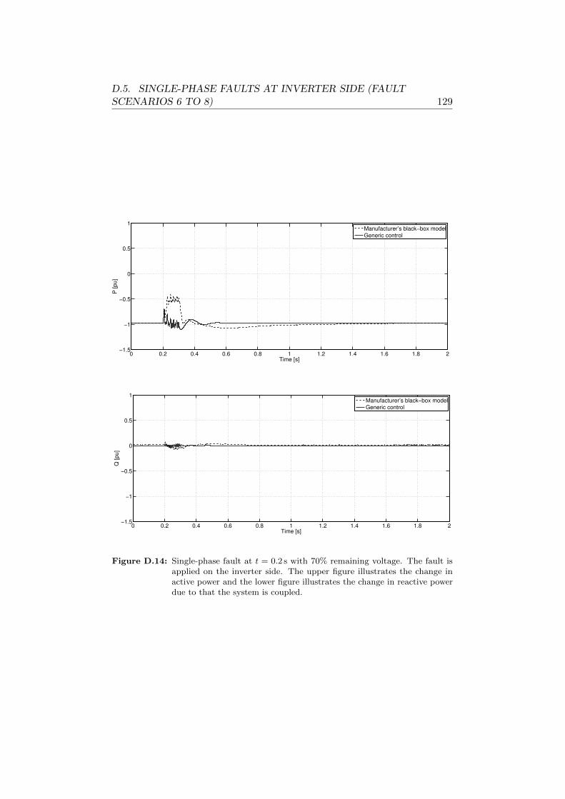
D.5. SINGLE-PHASE FAULTS AT INVERTER SIDE (FAULTSCENARIOS 6 TO 8) 129
0 0.2 0.4 0.6 0.8 1 1.2 1.4 1.6 1.8 2−1.5
−1
−0.5
0
0.5
1
Time [s]
P [
pu
]
Manufacturer’s black−box modelGeneric control
0 0.2 0.4 0.6 0.8 1 1.2 1.4 1.6 1.8 2−1.5
−1
−0.5
0
0.5
1
Time [s]
Q [pu]
Manufacturer’s black−box modelGeneric control
Figure D.14: Single-phase fault at t = 0.2 s with 70% remaining voltage. The fault isapplied on the inverter side. The upper figure illustrates the change inactive power and the lower figure illustrates the change in reactive powerdue to that the system is coupled.


![Fault-Line Identification of HVDC Transmission Lines by ...ppong/manuscripts/fault line identification HVDC transmission...HVDC system which was established in PSCAD/EMTDC [12] based](https://static.fdocuments.us/doc/165x107/5e69f3c1518f27522a452b9a/fault-line-identification-of-hvdc-transmission-lines-by-ppongmanuscriptsfault.jpg)