Vrije Universiteit Brussel

On-line Identification of the LC Product in Coupled Resonant CircuitsDe Angelis, Guido; De Angelis, Alessio; Moschitta, Antonio; Carbone, Paolo; Pintelon, Rik

Published in:IEEE Transactions on Instrumentation and measurement

DOI:10.1109/TIM.2019.2950583

Publication date:2020

Document Version:Submitted manuscript

Link to publication

Citation for published version (APA):De Angelis, G., De Angelis, A., Moschitta, A., Carbone, P., & Pintelon, R. (2020). On-line Identification of the LCProduct in Coupled Resonant Circuits. IEEE Transactions on Instrumentation and measurement, 69(7), 4592-4603. [8887191]. https://doi.org/10.1109/TIM.2019.2950583

General rightsCopyright and moral rights for the publications made accessible in the public portal are retained by the authors and/or other copyright ownersand it is a condition of accessing publications that users recognise and abide by the legal requirements associated with these rights.

• Users may download and print one copy of any publication from the public portal for the purpose of private study or research. • You may not further distribute the material or use it for any profit-making activity or commercial gain • You may freely distribute the URL identifying the publication in the public portalTake down policyIf you believe that this document breaches copyright please contact us providing details, and we will remove access to the work immediatelyand investigate your claim.

Download date: 18. Nov. 2021

1

On-line Identification of the LC Productin Coupled Resonant Circuits

Guido De Angelis, Alessio De Angelis, Antonio Moschitta, Paolo Carbone, Rik Pintelon

Abstract—We present an in-circuit approach for estimating theLC parameter in coupled resonant circuits. The theoretical back-ground is discussed by presenting the models and performing anumerical sensitivity analysis. The method for estimating LC isbased on noisy frequency response function measurements of thecoupled resonant circuit. A practical implementation is presentedand employed to validate the proposed method. Experimentalresults show that the proposed method provides an estimate ofLC with a deviation of less than 4% with respect to LCR metermeasurement results.

Index Terms—inductive coupling, magnetic fields, frequencyresponse function, frequency-domain system identification

I. INTRODUCTION

Resonant RLC circuits have gained more attention in thelast decade in many fields, such as power transfer [1],Biomedical systems [2]-[4], and Magnetic Positioning Systems(MPSs) [5]-[8]. In particular, MPSs are an interesting fieldof application and often rely on inductively coupled setsof high-Q resonant coils, as resonance can be exploited tocompensate for the distance-related attenuation and extend thesystem range. These systems usually measure the Vrms of thereceived signals and estimate ranges by inverting a suitablemagnetic field propagation model. The usage of an equivalentcircuit modeling the interaction between two coils allowsthe inversion of the model that requires knowledge of theparameters related to physical properties of the coupled coils.Thus, a properly characterized equivalent model can supportimproved accuracy, system deployment and tuning. In fact, dueto fabrication tolerances, the actual characteristics of a realizedcoil will slightly differ from the nominal value. Consequently,if nominal values are used in the propagation model, anuncertainty source is introduced that adversely affects positionmeasurements. Hence, accurate parametric characterization ofa real system can be used as a calibration tool, improvingMPSs’ ranging and positioning accuracy. Moreover, sincethese parameters can change over time due to aging andother effects, calibration should be performed online withoutmodifying the system hardware.

The identification of the circuit parameters can often beperformed under simplifying assumptions. For instance, it was

This research activity was funded through grant PRIN 2015C37B25 bythe Italian Ministry of Instruction, University and Research (MIUR), whosesupport the authors gratefully acknowledge

G. De Angelis is with Regione Umbria, Perugia, ItalyA. De Angelis, A. Moschitta, and P. Carbone are with the Engineering

Department, University of Perugia, via G. Duranti 93, 06125 Perugia, Italy.alessio.deangelis, antonio.moschitta, paolo.carbone@unipg.it

R. Pintelon is with Department ELEC, Vrije Universiteit Brussel, Pleinlaan2, B1050 Brussels, Belgium.

shown in [5] that the RLC circuit parameters, including themutual inductance between the coils, depend only on thecoils’ relative orientation and on the distance between thecoils’ centers. For the purpose of estimating the position inan MPS, it was also shown that the information associatedwith the circuit parameters can be summarized by a con-stant, estimated in a preliminary calibration phase, and bythe mutual inductance between the coils. It is worth notingthat the estimation of the RLC circuit can be affected byvarious sources of uncertainty, that include parasitic effects,component tolerances, and environmental conditions [7].

In the literature, the problem of estimating offline thevalues of lumped components, resonant frequency, and Q-factor in RLC circuits is widely studied. In [9], the componentparameters are estimated using the vector fitting algorithmbased on a Least Squares approach. This algorithm processes aset of impedance measurements at several frequencies, appliesvector fitting recursively, and identifies lumped componentparameters. In [10], the authors estimate the inductance asa function of the physical coil parameters, i.e., diameter andnumber of turns. Moreover, in [11], the authors use a networkanalyzer to estimate the Q-factor for microwave applications.In [12], the Q-factor, the resonance frequency and the couplingcoefficient of a single resonator are measured through aninductively coupled sensor. Furthermore, in [13], a sensorreadout system based on impedance measurement is proposed.The system performs the impedance measurement using acapacitor discharge and a readout coil that is inductivelycoupled with the LC sensor. However, none of the mentionedreferences presents a procedure to perform an online paramet-ric identification.

This paper is focused on the identification of the productLC in an equivalent RLC circuit that models the interac-tion between two inductively coupled coils. Extending thepreliminary results in [14], we employ input-output voltagemeasurements to estimate the frequency response function(FRF) of the circuit and identify the coefficients of its transferfunction using frequency-domain techniques.

The procedure described in this paper extends publishedresults by adopting a frequency-domain system identificationtechnique enabling estimation and monitoring of the RLCparameters in an online and in-circuit fashion. Thus, discon-nection of the measured circuit is not required when applyingthe measurement procedure.

This paper is structured as follows: In Section II, theconsidered circuit is described and the proposed parametricidentification procedure is illustrated, including a comparisonto related approaches from the literature. Next, the background

2

Fig. 1. Picture of the hardware setup, showing two inductively coupled coils.

+

−VI

i0

RC

i1

C1

RL

i2

L1

RL

L2

RC

C2

i3

M Vrx

Fig. 2. Equivalent circuit of the coupled resonating coils.

theory and the derivation of the proposed identification methodare introduced in Section III. Results of a numerical sensitivityanalysis are discussed in Section IV. Furthermore, an exper-imental evaluation is presented in Section V and conclusionsare drawn in Section VI.

II. CONSIDERED CIRCUIT AND PARAMETERIDENTIFICATION METHOD

The circuit model considered in this paper includes twoinductively coupled coils, like those shown in Fig 1. Thecircuit parameters take into account the physical dimensionsof the coils (radius, height, thickness). The relative positionsof the coil centers and the coil orientations affect the valueof the mutual inductance. The coils are connected to lumpedcapacitors thus implementing resonators.

In the general case, the resonant circuits may be connectedin four configurations: parallel-parallel (PP), series-series (SS),series-parallel (SP), and parallel-series (PS). As an example,the circuit in Fig. 2 is connected in the PP configuration, sincethe equivalent circuit modeling the capacitor (C1,RC) is inparallel with the equivalent circuit of the inductor at one ofthe coils’ sides (L1, RL) and because the same applies to L2,RL and C2, RC . The other configurations are presented andanalyzed in the following section, where the correspondingschematic diagrams are also depicted in Fig. 7.

We make the simplifying assumption that both inductorshave the same value, i.e. L1 = L2 = L, and similarly for thecapacitors, i.e. C1 = C2 = C. If these values are different,then the frequency response of the overall circuit may exhibittwo resonance peaks. However, the frequency response of thecircuit still exhibits a single resonance peak if the Q-factor

frequency [Hz] #1043.5 4 4.5 5 5.5 6 6.5 7 7.5

Mag

nitu

de [d

B]

-60

-55

-50

-45

-40

-35

-30

-25

-20

-15

"LC

=-0.4

"LC

=-0.2

"LC

= 0

"LC

= 0.2

"LC

= 0.4

Fig. 3. Numerical simulation results of the SP configuration. Behavior ofthe transfer function for several values of the difference between the LCproducts of the two coupled resonators in the series-parallel configuration.When ∆LC = 0.4 and ∆LC = −0.4, the two resonance peaks are clearlyvisible.

of the resonators is of the order of magnitude of 10 and thedifference between the product L1C1 and the product L2C2,which we denote as ∆LC , is smaller than 20%, i.e.

|∆LC | , |(L1C1 − L2C2) /L1C1| < 0.2.

This behavior is illustrated by the numerical simulation resultsshown in Figs. 3 and 4. The numerical simulations have beenperformed in the SP configuration with the following values ofthe circuit parameters: M = 50.0134 nH; L1 = 30.19 µH; C1

= 303.76 nF; RL1 = 0.8968 Ω; RC1 = 0.1851 Ω; C2 = 311.37nF; RL2 = 0.9273 Ω; RC2 = 0.1777 Ω. Furthermore, thesimulations have been performed for different values of the L2

parameter, from 6 µH to 53 µH, resulting in a range of ∆LC

values from -0.8 to 0.8. The simulated values are consistentwith measurements performed on a realized prototype andreported in Section V of the present paper. Since the overallcircuit exhibits a single resonance peak, it is reasonable toassume equal values of the inductors and capacitors. Thus,the presented simulation results show that the approximationis valid.

In this paper, we derive the transfer function and the expres-sion for the LC parameter for all four possible configurations.We also report experimental estimates of the LC parameterin the PP configuration, which is widely used for magneticpositioning applications [8]. The proposed technique can beadapted for the other configurations as well.

The novelty of this paper, with respect to the other ap-proaches recalled in Section I, consists in the application ofan online frequency-domain system identification techniqueto the problem at hand. Accordingly, it is possible to im-plement online and in-circuit monitoring of the parametersfor fault detection applications. The proposed online and in-circuit estimation procedure is applied while the system isoperational. Such a procedure is based on input-output voltagemeasurements, which are performed without using externalinstrumentation or disconnecting the components from thecircuit under test, as done for instance in [15].

The method proposed in this paper estimates the LC param-eter of coupled resonant circuits using a multisine excitation.

3

Fig. 4. Numerical simulation results of the SP configuration. Pseudo-colorrepresentation of the behavior of the transfer function for ∆LC ranging from-0.8 to 0.8, obtained by varying the value of L2 and keeping the other circuitparameters constant. It is possible to notice that a single resonance peak ispresent for |∆LC | < 0.2, whereas two resonance peaks can be obseved for|∆LC | > 0.2.

Fig. 5. Block diagram of the considered system acquiring the input-outputvoltage signals of a coupled-inductors resonant circuit.

Frequency-domain system identification techniques are used toidentify the coefficients of the transfer function and to relatethem to the LC parameter [16].

Since it is only based on input and output voltage measure-ments, the proposed method does not require any hardwaremodification of the considered RLC circuit, such as the in-sertion of current-measurement shunt-resistors for impedanceevaluation [15], which cause Q-factor deterioration and perfor-mance degradation of the resonant circuits. Therefore, since itis an in-circuit measurement method, it can be used for on-line monitoring of faults that cause deviation of the circuitfrom its nominal characteristic, e.g. due to component agingor environmental factors.

Another possible application is the automatic tuning ofcoupled resonators, which could be especially beneficial foroptimizing the operational range and performance of magneticpositioning or wireless power transfer systems.

Furthermore, the proposed method provides the followingnovelties compared with the existing in-circuit identification

VI Z1

Z2

Z3

Z4

Z5 Vrx

Fig. 6. Equivalent T circuit of the coupled resonating coils, showing thebranch impedances Zi.

techniques: (i) the identification model includes noise effectson both the input and output voltage measurements, and (ii)detection and quantification of the nonlinear distortions isenabled by the usage of multisine excitations and system-identification techniques. This latter feature allows setting thevalidity limits of the linear approximation in the analysis ofthe tested circuit [16].

A block diagram illustrating the architecture of the proposedmeasurement system is depicted in Fig. 5. The input signalprovided by a signal generator to one of the two inductively-coupled resonant circuits is digitized by a data acquisitionsystem. Simultaneously, the output signal at the other resonatoris amplified by an instrumentation amplifier and digitized by asecond channel of the acquisition system. The digitized signalsare then transferred to a PC for further processing. In thefollowing section, the theoretical measurement principles aredescribed in detail.

III. THEORETICAL MEASUREMENT PRINCIPLES

In this section, we derive the transfer function of the equiva-lent circuit considered, in all four configurations. Furthermore,we derive an expression of the LC parameter.

A. Analysis of the Equivalent Circuit

A schematic of the RLC circuit in the PP configuration isshown in Fig. 2. As discussed in Section II, the circuit canbe analyzed under the simplifying assumptions C = C1 = C2

and L = L1 = L2 as in [5]. In particular, we can define:

Z1(s) = Z5(s) = RC +1

sCZ4(s) = Z2(s) = RL + s(L−M)

Z3(s) = sM,

(1)

where Zi, with i = 1 . . . 5, is the impedance of each circuitbranch of the equivalent T circuit depicted in Fig. 6. Theparasitic resistances of the coils and the capacitors are shownas RL and RC , respectively. The resistor denoted as RC isthe equivalent series resistor (ESR), which is widely used inthe literature to represent the losses of a capacitor.

To analyze this circuit, we derived analytical expressionsand validated them using the ac analysis tool of SPICE, thewidely used circuit simulator. The SPICE schematic used inthe simulations, which contains resistors, capacitors, inductors,

4

(a) PP circuit configuration. (b) SS circuit configuration.

(c) SP circuit configuration. (d) PS circuit configuration.

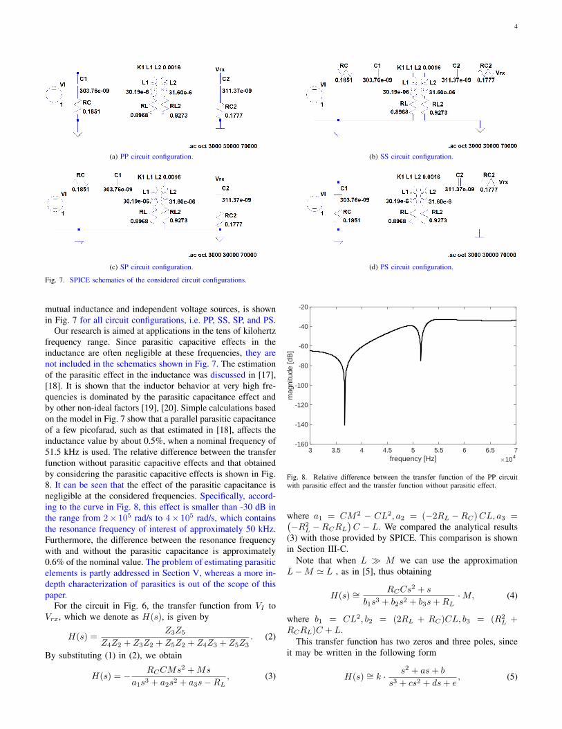
Fig. 7. SPICE schematics of the considered circuit configurations.

mutual inductance and independent voltage sources, is shownin Fig. 7 for all circuit configurations, i.e. PP, SS, SP, and PS.

Our research is aimed at applications in the tens of kilohertzfrequency range. Since parasitic capacitive effects in theinductance are often negligible at these frequencies, they arenot included in the schematics shown in Fig. 7. The estimationof the parasitic effect in the inductance was discussed in [17],[18]. It is shown that the inductor behavior at very high fre-quencies is dominated by the parasitic capacitance effect andby other non-ideal factors [19], [20]. Simple calculations basedon the model in Fig. 7 show that a parallel parasitic capacitanceof a few picofarad, such as that estimated in [18], affects theinductance value by about 0.5%, when a nominal frequency of51.5 kHz is used. The relative difference between the transferfunction without parasitic capacitive effects and that obtainedby considering the parasitic capacitive effects is shown in Fig.8. It can be seen that the effect of the parasitic capacitance isnegligible at the considered frequencies. Specifically, accord-ing to the curve in Fig. 8, this effect is smaller than -30 dB inthe range from 2× 105 rad/s to 4× 105 rad/s, which containsthe resonance frequency of interest of approximately 50 kHz.Furthermore, the difference between the resonance frequencywith and without the parasitic capacitance is approximately0.6% of the nominal value. The problem of estimating parasiticelements is partly addressed in Section V, whereas a more in-depth characterization of parasitics is out of the scope of thispaper.

For the circuit in Fig. 6, the transfer function from VI toVrx, which we denote as H(s), is given by

H(s) =Z3Z5

Z4Z2 + Z3Z2 + Z5Z2 + Z4Z3 + Z5Z3. (2)

By substituting (1) in (2), we obtain

H(s) = − RCCMs2 +Ms

a1s3 + a2s2 + a3s−RL, (3)

frequency [Hz] #1043 3.5 4 4.5 5 5.5 6 6.5 7

mag

nitu

de [d

B]

-160

-140

-120

-100

-80

-60

-40

-20

Fig. 8. Relative difference between the transfer function of the PP circuitwith parasitic effect and the transfer function without parasitic effect.

where a1 = CM2 − CL2, a2 = (−2RL −RC)CL, a3 =(−R2

L −RCRL)C − L. We compared the analytical results

(3) with those provided by SPICE. This comparison is shownin Section III-C.

Note that when L M we can use the approximationL−M ' L , as in [5], thus obtaining

H(s) ∼=RCCs

2 + s

b1s3 + b2s2 + b3s+RL·M, (4)

where b1 = CL2, b2 = (2RL + RC)CL, b3 = (R2L +

RCRL)C + L.

This transfer function has two zeros and three poles, sinceit may be written in the following form

H(s) ∼= k · s2 + as+ b

s3 + cs2 + ds+ e, (5)

5

where

k =MRCL2

(6)

a =1

CRC(7)

b = 0 (8)

c =2RL +RC

L(9)

d =

(R2L +RCRL

)C + L

CL2(10)

e =RLCL2

. (11)

B. Analytical solution for the product LC

We may write (5) in a more convenient form by factoringthe denominator as follows

H(s) ∼= k · s2 + as

(s+ α) (s2 + βs+ γ), (12)

where

α =RLL

(13)

β =RC +RL

L(14)

γ =1

LC. (15)

Notice that this model is not identifiable, i.e., it is notpossible to univocally calculate the parameters M , L, C, RC ,and RL by estimating the coefficients of the transfer functionin (12). In fact, the nonlinear system of equations given by(6), (7), (13), (14), and (15), where M , L, C, RC , and RLare the unknowns, admits an infinite set of solutions, givenby ξM0, ξL0, C0/ξ, ξRC0, ξRL0, for any ξ ∈ R and ξ 6= 0.Here, M0, L0, C0, RC0, and RL0 are the nominal values ofthe circuit parameters.

In addition to the identifiability issue, another problem isthe presence of strongly nonlinear functions in the expressionsof the coefficients of (12). Even if the model was identifiable,solving for the unknowns would require a numerical approach,with close-to-the-solution initial values, to avoid local minima.

However, the product LC is identifiable. In fact, by mea-suring the FRF of the circuit and performing a parametricidentification of the coefficients of (12), the product LC canbe estimated by direct inversion of the γ coefficient in (15).

C. Transfer functions for the SS, SP, and PS configurations

In this section, we provide the analytical expressions of thetransfer functions and the formulas for calculating the LCparameter for the SS, SP, and PS configurations. These transferfunctions were obtained using the ABCD matrix method [21].Detailed derivations are provided in the Appendix. The transferfunction of the SS circuit is given by

HSS(s) =MCs2

s2CL+ sC(RL +RC) + 1. (16)

In this configuration, LC is given directly by the denominatorcoefficient of s2.

frequency [Hz] #1043 3.5 4 4.5 5 5.5 6 6.5 7

mag

nitu

de [d

B]

-60

-50

-40

-30

-20

-10

PS circuitSP circuitPP circuitSS circuit

Fig. 9. Transfer function of the PS, SP, PP, and SS circuits. The color linesdenote the analytical expressions, while the black lines indicate the results ofthe circuit simulation (SPICE).

Moreover, the SP circuit has the following transfer function

HSP (s) = − g3s3 + g2s

2

f4s4 + f3s3 + f2s2 + f1s− 1, (17)

where g3 = C2MRC , g2 = CM , f4 = C2M2 −C2L2, f3 =−2C2LRL−2C2LRC , f2 = −C2R2

L−2C2RCRL−C2R2C−

2CL and f1 = −2CRL−2CRC . In the SP configuration, theparameter LC is given by LC =

√g22 − f4.

Finally, the transfer function of the PS circuit is given by

HPS(s) =Ms

Ls+RL. (18)

Notice that it is impossible to estimate the LC product inthe PS configuration, since C does not appear in the transferfunction expression. In this configuration, resonance does notoccur.

By numerically evaluating the above transfer functions, weobtain the plots shown in Fig. 9. Note that, at least around theresonance frequency, the behavior of the SS and PP circuits issimilar. Moreover, from Fig. 9 it can be observed that the PScircuit is not resonant, thus validating the theoretical derivationin (18). Finally, a good agreement between the curves obtainedby circuit simulation and those obtained by the analyticalexpressions can be noticed. The small differences betweenthose curves are due to the fact that the circuit simulationswere performed with the parameter values shown in Fig. 7,whereas the analytical expressions use the simplifying assump-tions L1 = L2 = L and C1 = C2 = C.

In the remainder of the paper, we focus on the PP circuit,which is widely used in MPS applications [5]. For thisconfiguration, we provide a numerical sensitivity analysis andexperimental results in the following sections.

IV. SENSITIVITY ANALYSIS

In this section, the sensitivity of the mathematical modelin (3) is analyzed by analytical derivations and by numericalsimulation. This analysis is useful, since it may consent toassess the tolerance requirement on the lumped componentsthat realize the MPS’s beacons and mobile nodes.

We recall that the sensitivity to the parameters is definedas the ratio between the percentage change in the transfer

6

function H and the percentage change in the parameter α,where α denotes any of the circuit parameters, i.e. α ∈M, C, L, RC , RL. Therefore, the formula for the sensi-tivity of H to the parameter α, denoted as SHα , is [22]:

SHα =∂H

∂α

α

H

∣∣∣∣α0

, (19)

with α0 the nominal value of the parameter α, in our case thetrue value of the circuit parameter used in the simulation.

By applying (19) to the expression of H(·) in (3), thesensitivity associated with the M parameter is:

SHM =∂H

∂M

M

H

∣∣∣∣M0

=SHM,1

SHM,2

, (20)

where

SHM,1 =−(CM2 + C L2

)s3 − (2CLRL + CLRC) s2

−(C RL

2 + C RCRL + L)s−RL

SHM,2 =(CM2 − C L2

)s3 + (−2CLRL − CLRC) s2

+(−C RL2 − C RCRL − L

)s−RL.

Furthermore, for the L parameter, we have that

SHL =SHL,1SHL,2

, (21)

where

SHL,1 =2C L2 s3 + (2CLRL + CLRC) s2 + Ls

SHL,2 =(CM2 − C L2

)s3 + (−2CLRL − CLRC) s2

+(−C RL2 − C RCRL − L

)s−RL.

For the C parameter, the following expression applies

SHC =SHC,1SHC,2

(22)

where

SHC,1 =−(CM2 − C L2

)s3 + 2CLRLs

2 − C RL2s

SHC,2 =(C2M2 − C2 L2

)RCs

4

+(−2C2LRCRL − C2LRC

2 + CM2 − C L2)s3

−(C2RCRL

2+(C2RC

2+2CL)RL + 2CLRC

)s2

+(−C RL2 − 2C RCRL − L

)s−RL.

Furthermore, for the RL parameter we obtain

SHRL=SHRL,1

SHRL,2

, (23)

where

SHRL,1 =2CLRLs2 +

(2C RL

2 + C RCRL)s+RL

SHRL,2 =(CM2 − C L2

)s3 + (−2CLRL − CLRC) s2

+(−C RL2 − C RCRL − L

)s−RL.

Finally, the expression for the RC parameter is

SHRC=SHRC ,1

SHRC ,2

, (24)

frequency [Hz]103 104 105 106

Sen

sitiv

ity fa

ctor

[dB

]

-140

-120

-100

-80

-60

-40

-20

0

20

MCLRCRL

Fig. 10. Sensitivity analysis of the model in (3) to the circuit parameters.

where

SHRC ,1 =(C2M2 − C2 L2

)RCs

4

− 2C2LRCRLs3 − C2RCRL

2s2

SHRC ,2 =(C2M2 − C2 L2

)RCs

4

+(−2C2LRCRL − C2LRC

2 + CM2 − C L2)s3

−(C2RCRL

2+(C2RC

2+2CL)RL + 2CLRC

)s2

+(−C RL2 − 2C RCRL − L

)s−RL.

The plots shown in Fig. 10 are obtained by numericalevaluation of (20)-(24) based on the following referencevalues: L = 30.887 µH, C = 307.54 nF, RL = 0.9119 Ω,RC = 0.1814 Ω and a mutual inductance M = 50.0134 nH.It can be inferred that the largest sensitivities are associatedwith the circuit inductance and capacitance, with a reducedsensitivity to parasitic resistances.

V. EXPERIMENTAL EVALUATION

To validate the proposed strategy for identifying the productLC, experiments were performed on a realized circuit. Suchcircuit consisted of the two coupled inductors depicted inFig. 1, each connected in parallel with a lumped capacitor,according to the schematic in Fig. 2. The two air-core coilswere realized by winding 20 turns of 0.25 mm diameter wireon cylindrical holders having a radius of 20 mm and a heightof 3.5 mm. The resulting nominal inductance of the coilswas L1 = L2 = L = 29 µH, calculated using Wheeler’sformula [23]. The nominal value of the lumped capacitors wasC1 = C2 = C = 330 nF. Therefore, the resonant frequencyof the realized circuit was approximately 53 kHz.

A. Stepped sine excitation for FRF measurement

In order to measure the FRF of the realized circuit, a steppedsine excitation was initially used. Specifically, one of the twocoils was connected to an an Agilent 33220A signal gener-ator. This generator was configured to provide a sinusoidalwaveform at a set of 81 frequencies. For each frequency, ameasurement of the RMS value of the induced voltage onthe other coil was performed, after amplifying the voltage atthe coil by means of an AD8421 instrumentation amplifierwith a gain of 40 dB. These RMS voltage measurements wereperformed using a Fluke 8845A Digital Multimeter.

7

frequency [Hz] #1043 3.5 4 4.5 5 5.5 6 6.5 7

mag

nitu

de [d

B]

-60

-55

-50

-45

-40

-35

-30

ExperimentalDataSpiceelis method 2/3elis method 5/6

Fig. 11. Experimental results. Magnitude of the measured FRF, that simulatedby Spice, that estimated using the elis 2/3 method and the elis 5/6 method.

The record of measurement results, of length 81, was subse-quently resampled by interpolation, using the Matlab functionresample, to obtain a record of 1000 values that was used forsubsequent identification. During the measurement procedure,the two coils were placed on the same plane, and the distancebetween their centers was 10 cm. The experimental resultsof the FRF measurement procedure are shown in Fig. 11,where an FRF obtained by the circuit simulator Spice usingthe nominal values of the components is also shown.

Furthermore, the measured frequency response function datawas fed to the elis (estimation of linear systems) algorithmfor parametric system identification, which is implementedin the frequency-domain identification Matlab toolbox fdident[24]. The elis algorithm is commonly used in the literaturefor system identification. It solves least squares estimationproblems employing the errors-in-variables model. Such amodel accounts for measurement errors in both the input andthe ouput of the system under test [16]. The elis algorithmwas configured for performing a model scan, i.e. identifyinga set of models differing by number of poles and zeros. Thescanned numbers of zeros are from 2 to 6, whereas the scannednumbers of poles are from 3 to 6. In the following, we presentresults for two of the scanned models. The first model, denotedas elis 2/3, is defined by two zeros and three poles, whichcorresponds to the number of poles and zeros of the idealmodel of the physical circuit in (3). The second model, denotedas elis 5/6, has five zeros and six poles, corresponding to themodel with the smallest error within the scanned set.

The results of the identification process are presented inFig. 11, Fig. 12, and Fig. 13. From these plots, a goodagreement can be observed between the experimental data andthe fitted curves, especially in the vicinity of the resonancefrequency. Specifically, Fig. 12 shows a difference of lessthan 1.5 dB between the measured FRF and that estimatedusing the elis 2/3 method and the elis 5/6 method. For thepurpose of shape comparison, here the maximum magnitude ofall the FRF curves was normalized to 1. Similar observationscan be obtained by the empirical cumulative density functionin Fig. 13. Therefore, the feasibility of the proposed fittingstrategy is validated.

frequency [Hz] #1043 3.5 4 4.5 5 5.5 6 6.5 7

mag

nitu

de [d

B]

-2

-1.5

-1

-0.5

0

0.5

1

1.5

Spiceelis method 2/3elis method 5/6

Fig. 12. Experimental results. Difference between the magnitude of themeasured FRF, that simulated by Spice, that estimated using the elis 2/3method and the elis 5/6 method.

magnitude [dB]-2 -1.5 -1 -0.5 0 0.5 1 1.5

CD

F

0

0.2

0.4

0.6

0.8

1

Spiceelis method 2/3elis method 5/6

Fig. 13. Empirical CDF of the difference between the magnitude of themeasured FRF, that simulated by Spice, that estimated using the elis 2/3method and the elis 5/6 method.

B. Multisine excitation for FRF measurement

The stepped sine excitation used in the previous subsectionfor measuring the FRF has the main drawback of requiringa relatively long measurement time. In fact, for each ofthe frequency steps desired, it is necessary to perform theentire measurement procedure and sufficient time should beemployed to allow for transients to vanish. To overcome thisdrawback, broadband excitations are often employed in prac-tical scenarios. In particular, periodic random-phase multisinesignals provide benefits such as the possibility of estimatingthe variance and the capability of detecting nonlinear distor-tions in the system [16].

For these reasons, an additional experimental test wasperformed, where the FRF was measured using a full random-phase multisine. The same circuit used in the previous subsec-tion, depicted in Fig. 1, was connected to a Keysight U2331Amultifunction data acquisition board, according to the blockdiagram of Fig. 5. The multisine excitation was generated bythe on-board 12-bit DAC and two acquisition channels wereused, for digitizing the input and output. Each channel wasacquired with a resolution of 12 bits and a sampling rateFs = 300 kSa/s, using coherent sampling with the acquisitionclock synchronized with the signal generation clock.

The input signal consisted of 300 periods of a random-phasemultisine synthesized using the Matlab fdident toolbox [24],with 1000 samples per period, containing all harmonics of the

8

fundamental frequency, which was equal to 300 Hz. The root-mean-square value of the input signal was 0.3 V. The effectof the transient was removed by discarding the first period ofthe acquired signals. For each of the remaining periods, thediscrete Fourier transform (DFT) was computed. Then, theobtained DFT sequences were averaged and used to obtain anestimate of the FRF using the maximum likelihood estimatordescribed in [16, chapter 2]. Such DFT sequences, which arerelated to repeated multisine measurements, were also used toobtain an estimate of the standard deviation of the FRF .

Two tests were performed: the first one was carried outwithout adding the instrumentation amplifier (INA) at theoutput of the system, therefore connecting the output of thereceiving resonator to the acquisition board directly. Thesecond test was performed by connecting the AD8421 INAwith a gain of 40 dB to the output, thus acquiring the signal atthe output of the INA. The results are shown in Fig. 14, whereboth the average and the standard deviation of the estimatedFRF are depicted. In the figure, the nominal gain value of40 dB is subtracted from the curve related to the INA results.

The purpose of the test carried out without the INA isto show which results can be achieved when an INA isnot available in the intended application, e.g. due to low-power requirements. It follows that even in this case it ispossible to estimate the transfer function in the vicinity ofthe resonance frequency, albeit with a degraded performancein terms of signal-to-noise ratio. Specifically, from Fig. 14, itcan be seen that the two curves obtained with and without theINA are in good agreement with each other in the frequencyband corresponding to the resonance peak of the system.However, the standard deviation obtained without the INA isapproximately 30 dB higher than that obtained using the INA.Furthermore, the average FRF is noisy outside the resonanceregion, thus preventing an accurate estimation outside suchregion.

The FRF measurement results obtained using the multisineexcitation were processed using the elis algorithm, obtainingthe results shown in Fig. 15 and Fig. 16, for the cases withoutand with the INA, respectively. It is possible to notice, fromFig. 16, that the 2-zero, 3-pole model corresponding to theideal circuit in (3) cannot accurately describe the FRF outsideof the resonance region. Therefore, a more complex model isneeded, with additional poles and zeros.

Such additional poles and zeros account for the effectof those parasitic components that are not included in theideal circuit model in (3). By increasing the model order, abetter fit of the experimental data is obtained, as shown byFig. 16. This means that the parasitic components result ina non-negligible contribution in those frequency ranges thatare outside of the resonance range. However, the presentedexperimental results prove that the simple ideal model is stillusable to identify the LC parameter without a significant lossof accuracy, because the transfer function in the resonanceregion is correctly described even by the 2-zero, 3-pole modelcorresponding to the ideal circuit of (3).

frequency [Hz] #1040 5 10 15

Mag

nitu

de [d

B]

-140

-120

-100

-80

-60

-40

-20frequency response function

average no INAstandard deviation no INAaverage INAstandard deviation INA

frequency [Hz] #1040 5 10 15

Pha

se [d

eg]

-500

-400

-300

-200

-100

0

100

200

300

400

average no INAaverage INA

Fig. 14. Experimental results. FRF measured using a multisine excitation.The average and standard deviation are obtained by considering 300 recordsof the acquired signals.

C. Evaluation of the analytical expression for the product LC

The denominator of the 2-zero, 3-pole model identified inthe previous subsection was factored in the form of (12), thusobtaining

H(s) =253.56s(s+ 6.859 · 105)

(s+ 5.693 · 104)(s2 + 3.142 · 104s+ 1.049 · 1011).

(25)

Therefore, an estimate of LC is obtained as LC =1/1.049 · 1011 = 9.5329 · 10−12.

To obtain an independent validation of this result, thelumped circuit components, i.e. capacitors and inductors, weredisconnected from the circuit and measured separately usingan LCR meter, the Iso-Tech LCR 821, with an uncertaintyof 0.05% [25]. The measurement procedure was performed at50 kHz. The measured values are shown in Table I. It maybe noticed that the measured value of C1 differs by 7.61 nFfrom the measured value of C2, while the difference betweenthe measured values of L1 and L2 is 1.41 µH. Therefore, thesimplifying assumptions of equal capacitance and inductancethat we made in Section III-A are valid, in the experimentalsetup, within an approximation error of 2.4% for C and 4.46%for L. Table I also presents the comparison between the valueof the product LC estimated by the proposed method and thatmeasured using the LCR meter considering the product L1C1

9

frequency [Hz] #1040 5 10 15

mag

nitu

de [d

B]

-110

-100

-90

-80

-70

-60

-50

-40

-30

experimental dataestimated transfer function 2/3error

(a)

frequency [Hz] #1040 5 10 15

mag

nitu

de [d

B]

-110

-100

-90

-80

-70

-60

-50

-40

-30

experimental dataestimated transfer function 5/6error

(b)

Fig. 15. Results of the parametric system identification using a multisine excitation without the INA. (a) 2-zero, 3-pole model; (b) 5-zero, 6-pole model.

frequency [Hz] #1040 5 10 15

mag

nitu

de [d

B]

-90

-80

-70

-60

-50

-40

-30

-20

-10

0

10

experimental dataestimated transfer function 2/3error

(a)

frequency [Hz] #1040 5 10 15

mag

nitu

de [d

B]

-90

-80

-70

-60

-50

-40

-30

-20

-10

0

10

experimental dataestimated transfer function 5/6error

(b)

Fig. 16. Results of the parametric system identification using a multisine excitation with the INA. (a) 2-zero, 3-pole model; (b) 5-zero, 6-pole model.

and the product L2C2. In both cases the proposed methodresults in a relative error of less than 3.95%.

D. Discussion of the results

The presented experimental results prove that the proposedin-circuit identification method is feasible in a practical sce-nario. In particular, the results show that the LC parameterof coupled resonating circuits is estimated within an error ofapproximately 4% with respect to an independent validationprocedure, which is performed using external instrumentationand disconnecting the individual components from the circuit.This independent validation procedure does not take intoaccount the parasitic behaviors that arise when the circuitcomponents are connected together during normal operationof the circuit. This fact partly explains the deviation in theestimate of the LC parameter. Moreover, with respect tothis independent validation procedure, the proposed online

method has the advantage of increased flexibility and possiblewidespread adoption in fault diagnosis scenarios.

The analysis provided in this paper assumes that onlyinput and ouput voltages are measured. If other quantitiesare measured, such as input current, output current, or volt-age across the individual reactive elements, then a differentanalysis should be carried out and possibly other circuitparameters may be identified. However, measuring currentstypically requires the usage of resistive shunts that degrade theperformance of the coupled circuits. Furthermore, measuringthe voltage across the individual reactive elements requiresadditional circuitry that increases the complexity and mayprevent online operation.

Potentially, the proposed in-circuit measurement method canbe implemented in real time for on-line fault detection. Inthis context, it could be used to monitor the behavior of theLC parameter over time and measure its deviation from thenominal value. Furthermore, the method could be applied to

10

TABLE IEXPERIMENTAL RESULTS. COMPARISON BETWEEN VALUES ESTIMATED

ACCORDING TO THE ANALYTICAL METHOD IN SECTION III-B ANDVALUES MEASURED USING AN LCR METER

measured estimated errorC1 [nF] 303.76 - -RC1 [Ω] 0.1851 - -L1 [µH] 30.19 - -RL1 [Ω] 0.8968 - -C2 [nF] 311.37 - -RC2 [Ω] 0.1777 - -L2 [µH] 31.60 - -RL2 [Ω] 0.9273 - -L1C1 [H·F] 9.1705E-12 9.5329E-12 3.6240E-13 (3.95 %)L2C2 [H·F] 9.8393E-12 9.5329E-12 -3.0640E-13 (-3.11 %)

resonance-based magnetic positioning systems to calibrate thecircuit parameters automatically, thus enhancing positioningaccuracy. Another possible application of the proposed methodis the automatic tuning of coupled resonators, which could beespecially beneficial for optimizing the operational range andperformance of wireless power transfer systems.

VI. CONCLUSION

In this paper, we considered a model of an RLC tuned-resonators equivalent circuit that has numerous practical ap-plications in the engineering field. We proposed an analyticalmethod for identifying the product LC based on the parametricidentification of the input-output voltage transfer function,which can be performed in-circuit without the need for ex-ternal instrumentation. The proposed method was applied toexperimental data resulting in a relative deviation of less than4% with respect to the values measured using an LCR meter,thus demonstrating its feasibility in a practical scenario.

APPENDIX

The equivalent electrical network of two coupled resonantcircuits is shown in Fig. 6 for the PP configuration. In thegeneral case, the network modeling the two resonant circuits isdecomposed into three blocks. The first block is the capacitiveimpedance in series or parallel with the second block, i.e., thecentral block, which represents the inductive impedance andthe mutual inductance (modeled by a T-network). Finally, thereis a third block, consisting of another capacitive impedance,which can be connected in series or parallel with the centralblock. In this way, it is possible to obtain diagrams that aresimilar to that of Fig. 6 for all four configurations. Afterperforming such a decomposition, the circuit can be analyzedin a simple fashion by using ABCD-parameters [21].

The ABCD-parameters, which are also known as chainparameters, are usually employed for representing cascadesof two-port networks. For a generic two-port network, shownin Fig. 17, the ABCD parameters are defined as follows:[

V1I1

]=

[A BC D

] [V2−I2

],

where V1 is the voltage at the input port, V2 is the voltage atthe output port, I1 is the current at the input port, and I2 isthe current at the output port.

Fig. 17. Diagram of a generic two-port network, showing the convention usedfor defining the ABCD parameters.

The cascade of our network is resulting in the followingexpressions

• PS circuit: FPS =

[1 01Z1

1

] [A BC D

] [1 Z5

0 1

];

• SP circuit: FSP =

[1 Z1

0 1

] [A BC D

] [1 01Z5

1

];

• SS circuit: FSS =

[1 Z1

0 1

] [A BC D

] [1 Z5

0 1

];

• PP circuit: FPP =

[1 01Z1

1

] [A BC D

] [1 01Z5

1

];

where FXX denotes the ABCD matrix of the XX circuit, withXX=PS, SP, SS, PP. Further, in a T-network, the elementsof the ABCD matrix are given as follows: A = 1 + Z2/Z3,B = Z2 + Z4 + (Z2 · Z4/Z3), C = 1/Z3 and D = 1 +Z4/Z3. Using the definitions in (1) of the Zi blocks, withi = 1 . . . 5, each transfer function HXX can be obtained byinverting the first element of the corresponding FXX matrix,i.e., HXX(s) = 1/FXX(1, 1) [21].

REFERENCES

[1] B. L. Cannon, J. F. Hoburg, D. D. Stancil, and S. C. Goldstein,“Magnetic resonant coupling as a potential means for wireless powertransfer to multiple small receivers,” IEEE Transactions on PowerElectronics, vol. 24, no. 7, pp. 1819–1825, July 2009.

[2] A. K. RamRakhyani, S. Mirabbasi, and M. Chiao, “Design and opti-mization of resonance-based efficient wireless power delivery systemsfor biomedical implants,” IEEE Transactions on Biomedical Circuits andSystems, vol. 5, no. 1, pp. 48–63, Feb 2011.

[3] M. Sawan, S. Hashemi, M. Sehil, F. Awwad, M. Hajj-Hassan, andA. Khouas, “Multicoils-based inductive links dedicated to powerup implantable medical devices: modeling, design and experimentalresults,” Biomedical Microdevices, vol. 11, no. 5, pp. 1059–1070, 2009.[Online]. Available: http://dx.doi.org/10.1007/s10544-009-9323-7

[4] E. Mattei, G. Calcagnini, F. Censi, M. Triventi, and P. Bartolini,“Numerical model for estimating rf-induced heating on a pacemakerimplant during mri: Experimental validation,” IEEE Transactions onBiomedical Engineering, vol. 57, no. 8, pp. 2045–2052, Aug 2010.

[5] G. De Angelis, A. De Angelis, A. Moschitta, and P. Carbone,“Comparison of measurement models for 3d magnetic localizationand tracking,” Sensors, vol. 17, no. 11, 2017. [Online]. Available:http://www.mdpi.com/1424-8220/17/11/2527

[6] S. Song, W. Qiao, B. Li, C. Hu, H. Ren, and M. Q. H. Meng, “Anefficient magnetic tracking method using uniaxial sensing coil,” IEEETransactions on Magnetics, vol. 50, no. 1, pp. 1–7, Jan 2014.

[7] V. Pasku, A. De Angelis, M. Dionigi, G. De Angelis, A. Moschitta, andP. Carbone, “A positioning system based on low-frequency magneticfields,” IEEE Transactions on Industrial Electronics, vol. 63, no. 4, pp.2457–2468, April 2016.

[8] V. Pasku, A. D. Angelis, G. D. Angelis, D. D. Arumugam, M. Dionigi,P. Carbone, A. Moschitta, and D. S. Ricketts, “Magnetic field-basedpositioning systems,” IEEE Communications Surveys Tutorials, vol. 19,no. 3, pp. 2003–2017, March 2017.

11

[9] P. M. Ramos and F. M. Janeiro, “Vector fitting based automatic circuitidentification,” in 2016 IEEE International Instrumentation and Mea-surement Technology Conference Proceedings, May 2016, pp. 1–6.

[10] M. Dionigi and M. Mongiardo, “Efficiency investigations for wirelessresonant energy links realized with resonant inductive coils,” in 2011German Microwave Conference, March 2011, pp. 1–4.

[11] K. J. Coakley, J. D. Splett, M. D. Janezic, and R. F. Kaiser, “Estimationof q-factors and resonant frequencies,” IEEE Transactions on MicrowaveTheory and Techniques, vol. 51, no. 3, pp. 862–868, March 2003.

[12] R. Nopper, R. Niekrawietz, and L. Reindl, “Wireless readout of passiveLC sensors,” IEEE Transactions on Instrumentation and Measurement,vol. 59, no. 9, pp. 2450–2457, Sept 2010.

[13] A. Babu and B. George, “An efficient readout scheme for simultaneousmeasurement from multiple wireless passive LC sensors,” IEEE Trans-actions on Instrumentation and Measurement, vol. 67, no. 5, pp. 1161–1168, May 2018.

[14] G. De Angelis, A. De Angelis, A. Moschitta and P. Carbone, “Iden-tification of resonant circuits’ parameters using weighted-least-squaresfitting,” in 2018 IEEE International Instrumentation and MeasurementTechnology Conference (I2MTC), May 2018.

[15] “Impedance measurement handbook. a guide to measurement technologyand techniques, 6th edition,” Keysight Technologies, Tech. Rep., 2016.

[16] R. Pintelon and J. Schoukens, System Identification: A FrequencyDomain Approach. Wiley, 2012.

[17] M. Bartoli, A. Reatti, and M. K. Kazimierczuk, “Modelling iron-powderinductors at high frequencies,” in Proceedings of 1994 IEEE IndustryApplications Society Annual Meeting, vol. 2, Oct 1994, pp. 1225–1232

vol.2.[18] A. Massarini and M. K. Kazimierczuk, “Self-capacitance of inductors,”

IEEE Transactions on Power Electronics, vol. 12, no. 4, pp. 671–676,July 1997.

[19] J. C. Hernandez, L. P. Petersen, and M. A. E. Andersen, “Low capacitiveinductors for fast switching devices in active power factor correction ap-plications,” in 2014 International Power Electronics Conference (IPEC-Hiroshima 2014 - ECCE ASIA), May 2014, pp. 3352–3357.

[20] S. R. Joaqun Bernal, Manuel J. Freire, “Use of mutual coupling todecrease parasitic inductance of shunt capacitor filters,” IEEE TRANS-ACTIONS ON ELECTROMAGNETIC COMPATIBILITY, vol. 57, no. 6,pp. 1408–1415, Dec 2015.

[21] D. A. Frickey, “Conversions between s, z, y, h, abcd, and t parameterswhich are valid for complex source and load impedances,” IEEETransactions on Microwave Theory and Techniques, vol. 42, no. 2, pp.205–211, Feb 1994.

[22] B. C. Kuo, Automatic Control Systems, 5th ed. Upper Saddle River,NJ, USA: Prentice Hall PTR, 1987.

[23] H. A. Wheeler, “Simple inductance formulas for radio coils,” Proceed-ings of the Institute of Radio Engineers, vol. 16, no. 10, pp. 1398–1400,Oct 1928.

[24] I. Kollar. (2004-2018) Fdident - frequency domain sys-tem identificaton toolbox for matlab. [Online]. Avail-able: https://www.mathworks.com/products/connections/product detail/frequency-domain-system-identification-toolbox.html

[25] Iso-Tech LCR 800 series user manual, https://docs-emea.rs-online.com/webdocs/0d82/0900766b80d82a9b.pdf.