VOT 74288

THE DEVELOPMENT OF MACHINE LEARNING BASED SOFTWARE

FOR PREDICTING PROTEIN-PROTEIN INTERACTIONS AND PROTEIN

FUNCTION FROM PROTEIN PRIMARY STRUCTURE

(PEMBANGUNAN PERISIAN BERASASKAN PEMBELAJARAN MESIN

UNTUK MERAMAL INTERAKSI PROTEIN-PROTEIN DAN FUNGSI

PROTEIN DARIPADA STRUKTUR PRIMARI PROTEIN)

MUHAMAD RAZIB BIN OTHMAN

SAFAAI BIN DERIS

HANY TAHER AHMED ALASHWAL

ROSLI BIN MD. ILLIAS

SAFIE BIN MAT YATIM

RESEARCH VOT NO:

74288

Jabatan Kejuruteraan Perisian

Fakulti Sains Komputer Dan Sistem Maklumat

Univerisit Teknologi Malaysia

2007

ii

ABSTRACT

Understanding proteins functions is a major goal in the post-genomic era.

Proteins usually work in context of other proteins and rarely function alone.

Therefore, it is highly relevant to study the interaction partners of a protein in order

to understand its function. For this reason, the main objective of this thesis is to

predict protein-protein interactions based only on protein primary structure. Using

the Support Vector Machines (SVM), different protein features have been studied

and examined. These features include protein domain structures, hydrophobicity and

amino acid compositions. The results imply that the protein domain structure is the

most informative feature for predicting protein-protein interactions. It also requires

much lower running time compared to the other features. However, using normal

binary SVM requires positive and negative data samples. Although it is easy to get a

dataset of interacting proteins as positive examples, there are no experimentally

confirmed non-interacting proteins to be considered as negative examples. Previous

researches cope with this problem by artificially generate random set of proteins

pairs that are not listed in the Database of Interacting Proteins (DIP) as negative

examples. This approach can be used for comparing features because the error will

be uniform. In this research, we consider this problem as a one-class classification

problem and solve it using the One-Class SVM. Using only positive examples

(interacting protein pairs) in training phase, the one-class SVM achieves accuracy of

80%. These results imply that protein-protein interaction can be predicted using one-

class classifier with comparable accuracy to the binary classifiers that use artificially

constructed negative examples. Finally, a Bayesian Kernel for SVM was

implemented to incorporate the probabilistic information about protein-protein

interactions that were compiled from different sources. The probabilistic output from

the Bayesian Kernel can assist the biologist to conduct more research on the highly

predicted interactions.

iii

ABSTRAK

Matlamat utama pada akhir era genom ialah memahami fungsi protein.

Kebiasaannya protein jarang berfungsi sendirian sebaliknya bekerja bersama protein

yang lain. Justeru, adalah sangat relevan mengkaji interaksi pasangan protein untuk

memahami fungsi protein tersebut. Maka, objektif utama tesis ini adalah untuk

meramal interaksi protein-protein berasaskan struktur pertama protein. Dengan

menggunakan Mesin Sokongan Vektor (SVM), ciri-ciri protein berlainan dapat dikaji

dan diuji. Ciri-ciri ini termasuklah struktur domain protein, hidrophobisiti dan

komposisi asid amino. Hasil kajian menunjukan bahawa struktur domain protein

mengandungi ciri maklumat yang paling berguna untuk meramal interaksi protein-

protein. Tambahan pula, ia memerlukan masa larian yang singkat berbanding ciri-ciri

yang lain. Namun demikian, penggunaan SVM binari normal memerlukan sampel

data positif dan negatif. Walaupun set data interaksi protein sebagai sampel positif

mudah diperolehi, namun tiada pengesahan melalui eksperimen bahawa protein yang

tidak-berinteraksi dianggap sebagai sampel negatif. Penyelidik terdahulu mengatasi

masalah ini dengan menjana set data pasangan protein yang tidak terkandung dalam

Pengkalan Data Interaksi Protein (DIP) secara rawak sebagai sampel negatif.

Pendekatan ini boleh digunakan untuk membandingkan ciri-ciri interaksi protein

disebabkan ralat yang seragam. Penyelidikan ini menganggap masalah tersebut

sebagai masalah pembahagian satu-kelas dan mengatasinya menggunakan SVM

Satu-Kelas. SVM Satu-Kelas mencapai ketepatan 80% jika hanya menggunakan

sampel positif (pasangan interaksi protein) dalam fasa latihan. Hasil kajian

merumuskan bahawa interaksi protein-protein boleh diramal menggunakan

pembahagian Satu-Kelas dengan lebih tepat berbanding pengelas binari yang

menggunakan binaan buatan sampel negatif. Seterusnya, Bayesian Kernel untuk

SVM diimplemetasi bagi menggabungkan kebarangkalian informasi tentang interaksi

protein-protein yang telah dikumpul dari pelbagai sumber. Kebarangkalian output

dari Bayesian Kernel dapat membantu ahli biologi untuk mengendalikan lebih

banyak penyelidikan tentang peramalan interaksi protein.

iv

TABLE OF CONTENTS

CHAPTER TITLE PAGE

ABSTRACT ii

ABSTRAK iii

TABLE OF CONTENTS iv

LIST OF TABLES vii

LIST OF FIGURES ix

LIST OF ABBREVIATIONS xii

CHAPTER 1 INTRODUCTION 1

1.1 Background of the Problem 1

1.2 Problem Statement 3

1.3 The Research Question 3

1.4 The Goal and Objectives 4

1.5 Importance of the Study 4

1.6 Scope of the study 6

1.7 Thesis Outline 7

1.8 Summary 9

CHAPTER 2 BASIC CONCEPTS IN MOLECULAR

BIOLOGY

10

2.1 The Central Dogma of Molecular Biology 10

2.2 The DNA 12

2.3 The Proteins 13

2.4 The Genetic Code 16

2.5 Proteins Functions 17

2.6 Protein-Protein Interactions 20

2.7 Summary 24

v

CHAPTER 3 LITERATURE REVIEW 25

3.1 Protein Function Prediction 25

3.2 Methods to study protein-protein interactions 30

3.3 Predicting Protein-Protein Interactions 32

3.4 Support Vector Machines 41

3.5 Bayesian Networks 43

3.6 Summary 46

CHAPTER 4 RESEARCH METHODOLGY 47

4.1 Research Design 47

4.2 General Research Framework 48

4.3 Protein Data Sets 51

4.4 Evaluation Measures of the System

Performance

54

4.5 Summary 56

CHAPTER 5

COMPARISON OF PROTEIN SEQUENC FEATURES FOR THE PREDICTION OF PROTEIN-PROTEIN INTERACTIONS USING SUPPORT VECTOR MACHINES

57

5.1 Related Work 57

5.2 Comparison Experiment Framework 60

5.3 The Support Vector Mahines 62

5.4 Features Representation 70

5.5 Materials and Implementation 72

5.5.1 Data Sets 72

5.5.2 Data Preprocessing 75

5.6 Results and Discussion 78

5.7 Summary 84

CHAPTER 6 ONE-CLASS SUPPORT VECTOR MACHINES FOR PROTEIN-PROTEIN INTERACTIONS PREDICTION

85

6.1 Related Work 85

6.2 One-Class Classification Problem 88

vi

6.3 One-Class Support Vector Machines 90

6.4 Datasets and Implementation 95

6.5 Results using Domain Feature 97

6.6 Results using Hydrophobicity Feature 101

6.7 Discussion 105

6.8 Summary 106

CHAPTER 7 REACTIVE CONSTRAINTS PROCESSING 107

ALGORITHMS

7.1 Related Work 107

7.2 Bayesian Approach 109

7.2.1 Bayesian Probability 109

7.2.2 Bayesian Networks 110

7.3 Kernel Methods 111

7.4 Bayesian Kernels 117

7.5 Bayesian Kernel for Protein-Protein

Interactions Prediction

119

7.6 Results and Discussion 121

7.7 Summary 127

CHAPTER 8 CONCLUSION AND FUTURE WORK 128

8.1 Conclusion 128

8.2 Research Contributions 131

8.3 Future Work 132

8.4 Closing 133

RELATED PUBLICATIONS 134

REFERENCES 136

vii

LIST OF TABLES

TABLE NO. TITLE PAGE

2.1 The amino acids. 14

2.2 The standard genetic code 17

2.3 Proteins functions 18

3.1 Computational methods for protein function prediction 30

3.2 High-throughput experimental approaches to the

determination of protein-protein interactions.

33

3.3 Computational methods for protein-protein interactions

prediction

36

4.1 The protein interactions of yeast Saccharomyces

cerevisiae identified by wet lab experiments.

51

4.2 The contingency table. 54

5.1 The classifier performance on domain structure feature

using 10-fold cross validation with variant threshold.

80

5.2 The classifier performance on domain structure with

scores feature using 10-fold cross validation with

variant threshold.

80

5.3 The classifier performance on hydrophobicity feature

using 10-fold cross validation with variant threshold.

81

5.4 The classifier performance on hydrophobicity with

scale feature using 10-fold cross validation with variant

threshold.

81

viii

5.5 The overall performance of SVM for predicting PPI

using domain and hydrophobicity features.

82

6.1 One-Class performance using different kernel with the

domain feature

101

6.2 One-Class performance using different kernel with the

domain feature.

104

7.1 Bayesian Kernel performance with varied threshold

using domain feature.

123

7.2 Bayesian Kernel performance compared to the standard

kernels using domain feature.

124

7.3 Performance comparison with the cited literature. 104

ix

LIST OF FIGURES

FIGURE NO. TITLE PAGE

2.1 The central dogma of molecular biology (Korf et al.,

2003).

11

2.2 Schematic drawing of protein secondary structure

(Punta and Rost, 2005).

15

2.3 The protein-protein interaction network in yeast

(Uetz, 2000).

21

2.4 (a) Large protein complex and its protein-protein

interactions.

(b) The schematic interaction (Cramer et al., 2001).

22

3.1 Different methods for inferring protein function. 26

3.2 The overlap between different high-throughput

experiments.

34

4.1 The general research operational framework. 50

4.2 A simplified entity-relationship diagram of the DIP

database (Xenarios et al., 2002).

53

5.1 The framework of comparing protein sequence

features. threshold.

61

5.2 (a) A separating hyperplane with small margin.

(b)A separating hyperplane with larger margin.

62

x

5.3 (a) Hard margin solution when data contain noise.

(b) Soft margin solution when data contain noise.

68

5.4 Part of the protein-protein interactions list from DIP. 73

5.5 Part of the protein-protein interactions list with

sequences name only.

74

5.6 Part of the protein sequence file. 75

5.7 Part of the protein domains file. 76

5.8 Part of the protein domains structure for the yeast

genome.

77

5.9 Part of the training data file. 77

5.10 The ROC curves and scores for predicting protein-

protein interactions.

83

6.1 Target and outlier classes in the one-class

classification problem.

89

6.2 Classification in the one-class SVM. 93

6.3 The implementation framework for the one-class

SVM.

96

6.4 The one-class SVM performance using domain

feature with the linear kernel.

99

6.5 The one-class SVM performance using domain

feature with the polynomial kernel.

99

6.6 The one-class SVM performance using domain

feature with the RBF kernel.

100

6.7 The one-class SVM performance using domain

feature with the sigmoid kernel.

100

xi

6.8 The one-class SVM performance using

hydrophobicity feature with the linear kernel.

102

6.9 The one-class SVM performance using

hydrophobicity feature with the polynomial kernel.

103

6.10 The one-class SVM performance using

hydrophobicity feature with the RBF kernel.

103

6.11 The one-class SVM performance using

hydrophobicity feature with the sigmoid kernel.

104

7.1 Illustration of mapping input data to a feature space. 113

7.2 The ROC curve for the Bayesian kernel and the

standards kernel.

124

7.3 The distribution of the probabilistic output for the

Bayesian kernel

104

xii

LIST OF ABBREVIATIONS

BN – Bayesian Networks

DIP – The Database of Interacting Proteins

DNA – Deoxyribonucleic Acid

DPEA – Domain Pair Exclusion Analysis

DPI – Dual Polarisation Interferometry

FNR – False Negative Rate

FPR – False Positive Rate

GO – Gene Ontology

HGP – Human Genome Project

InterDom – The Database of Interacting Domains

KBM – Kernel Based Methods

KM – Kernel Matrix

LIBSVM – Library for Support Vector Machine

MIPS – Munich Information Center for Protein Sequences

mRNA – Messenger Ribonucleic Acid

MSSC – Maximum Specificity Set Cover

ncRNA – Non-coding Ribonucleic Acid

PDB – Protein Data Bank

PFAM – Protein Families Database

PID – Potentially Interacting Domain

PIE – Probabilistic Interactome Experimental

PPI – Protein-Protein Interactions

QP – Quadratic Programming

RBF – Radial Basis Function

RNA – Ribonucleic Acid

RNAi – Ribonucleic Acid inference mechanism

xiii

ROC – Receiver Operating Characteristic

RVM – Relevance Vector Machine

SGD – Saccharomyces Genome Database

SVM – Support Vector Machines

TAP – Tandem Affinity Purification

TPR – True Positive Rate

YPD – The Yeast Proteome Database

CHAPTER 1

INTRODUCTION

Bioinformatics or computational biology is broadly defined as the application

of computational techniques to solve biological problems. This field has arisen in

parallel with the development of automated high throughput methods of biological

and biochemical discovery that yield a huge and variety forms of experimental data,

such as DNA and protein sequences, gene expression patterns, and chemical

structures. Major research efforts in bioinformatics include sequence alignment, gene

finding, genome assembly, protein structure alignment, protein structure prediction

and prediction of protein-protein interactions. In this thesis, the prediction of protein-

protein interactions from sequences data using machine learning techniques is

presented. The background of the problem, objectives, importance of the study, and

the scope of this research is presented and discussed in this chapter.

1.1 Background of the Problem

The majority of functions in cells are accomplished by proteins. Therefore,

assigning functions to the proteins encoded by a genome is one of the crucial steps in

gaining understanding of the organism. Because the function of half of all proteins in

newly sequenced genomes often is completely unknown, complete genome

sequencing gives much less insight into the organism than initially hoped for

(Walhout and Vidal, 2001). Although, most methods annotating protein function

2

utilise sequence homology to proteins of experimentally known function, such a

homology-based annotation transfer is problematic and limited in scope. Therefore,

alternative approaches have begun to develop. These approaches include methods

based on phylogenetic patterns, gene expression, and protein-protein interactions

data.

The sequencing of entire genomes has moved the attention from the study of

single proteins or small complexes to that of the entire proteome. Most proteins do

not function in isolation, but collaborate with other proteins. In this context,

identifying protein-protein interactions (PPI) is an important goal of proteomics.

Protein-protein interactions data can help researchers to infer protein's functions

based on the information available about its partner. Usually, laboratory experiments

are used such as yeast two-hybrid analysis, protein microarrays and immunoaffinity

chromatography followed by mass spectrometry. Recently, computational methods

have been introduced because laboratory experiments are costly, time-consuming

and suffer from high false positive rates.

Part of the reason why it is difficult to relate the chemical function of a

protein to its biological purpose using homology-based annotation is that proteins do

not function alone. To understand the function of a protein, it must be considered in

its proper cellular context, for example by appreciating how the cell would behave

without it (Attwood and Miller, 2001). Many proteins are parts of larger complexes,

which are the functional units that fulfill a role in the cell (Gavin et al., 2002). In this

regard it can be argued that knowing proteins partners can give important clue about

its function. Therefore it is highly relevant to study the interaction partners of a

protein in order to understand its function (Ho et al., 2002) (Deng et al., 2002).

Most protein-protein interactions have been discovered by laboratory

techniques such as yeast two-hybrid system that can detect all possible combinations

of interactions. However, these findings can be superfluous and the number of

experimentally determined structures for protein-protein interactions is still quite

small. As a result, methods for computational prediction of protein-protein

interactions are becoming increasingly important.

3

Therefore the aim of this research is to predict protein-protein interactions

from protein primary structure data using machine learning techniques. Then the

availability of both the experimental and the predicted protein-protein interactions

data can be used to construct more reliable dataset for the prediction of proteins

functions.

1.2 Problem Statement

The research problem that we are trying to solve in this research can be

described as following. Given the protein-protein interactions data for the budding

yeast, Saccharomyces cerevisiae that are listed in the Database of Interacting

Proteins (DIP) and its protein sequences data, it is a challenging task to accurately

predict new protein-protein interactions based on that data using machine learning

techniques.

1.3 The Research Question

The main research question is:

How can the protein-protein interactions be predicted from protein sequences

data using machine learning techniques?

Thus, the following issues will arise to answer the main research question

stated above:

• How to identify the best protein sequence features that can be used to

train the learning algorithm?

• How to overcome the unavailability of confirmed non-interacting proteins

which is important as negative examples for the training of the learning

algorithm?

4

• How to incorporate the probabilistic protein-protein interactions

information to improve the prediction accuracy?

1.4 The Goal and Objectives

The main goal of this research is to develop a computational technique using

the Support Vector Machines (SVM) and Bayesian approach to predict protein-

protein interactions form protein sequences data of the budding yeast,

Saccharomyces cerevisiae.

To achieve this goal the following objectives have been set:

• To investigate different protein sequence features for the prediction of

protein-protein interactions using the support vector machines.

• To formulate the problem of predicting protein-protein interactions as a

one-class classification problem then solve it using the One-Class SVM

• To incorporate the probabilistic protein-protein interactions information

using Bayesian kernel.

• To test, evaluate, and enhance the prediction system.

1.5 Importance of the Study

Assigning functions to the proteins encoded by a genome is one of the crucial

steps in gaining understanding of the organism. Besides, the study of protein function

is fundamental to the drug discovery process. However, the function of half of all

proteins in newly sequenced genomes often is completely unknown (Walhout and

Vidal, 2001). Therefore, assigning function to the newly discovered proteins

represents a major challenge in the post-genomic era, and could help biologists to

better understand the molecular mechanisms of biological events.

5

The most common approach to identify protein function is based on sequence

similarity. However, about 30% to 40% of the newly discovered proteins can not be

assigned function based on sequence homology or similarity because they do not

have statistically significant similarity with known protein (Letovsky and Kasif,

2003).

Inferring protein function can be made via protein-protein interaction studies.

This is due to the fact that proteins work in a context of other proteins and rarely

work alone. Hence, the function of unknown protein may be discovered if

information about its interaction partners of known function is available. For that

reason, the study of protein interactions has been fundamental to the understanding

of how proteins function within the cell. Characterizing the interactions of proteins in

a given cellular proteome will be the next milestone along the road to understanding

the biochemistry of the cell. As a result, studying protein-protein interactions to gain

insight on protein functions has become a topic of enormous interest in recent years,

resulting many efforts devoted to its research.

The interactions between proteins are important for many biological

functions. Almost all processes in of molecular biology are affected by protein-

protein interactions (Alberts et al. 2002, Lodish et al. 2004). Replication,

transcription, translation, signal transduction, protein trafficking, and protein

degradation are all accomplished by protein complexes, often temporally assembled

and disassembled to accomplish vital processes. In fact, the importance of protein–

protein interactions in the post-genomic era is becoming more noticeable due to the

huge volume of data that became available. Hence, studying protein-protein

interactions is crucial to gain insight on protein functions of the newly sequenced

genomes.

Until recently, information about protein–protein interactions was gathered

via experiments that were individually designed to identify and validate a small

number of specifically targeted interactions (Legrain et al., 2001). This type of

experiments is called small-scale experiments. This traditional source of information

has been increased recently by the results of high-throughput experiments designed

to exhaustively explore all the potential interactions within entire genomes.

6

However, the many discrepancies between the interacting partners identified in high-

throughput studies and those identified in small-scale experiments highlight the need

for caution when interpreting results from high-throughput studies (Salwinski and

Eisenberg 2003).

These discrepancies represent the need for the development of computational

methods for data validation. Indeed, the interaction data that have been provided by

high throughput technologies like the yeast two-hybrid system are known to suffer

from many false positives. In addition, in vivo experiments elucidating protein-

protein interactions are still time-consuming and labor-intensive methods. As a

result, complementary computationally methods capable of accurately predicting

interactions would be of considerable value. Furthermore, computational methods for

the prediction of protein interactions will provide more data which will enable

predicting protein function more precisely since the function of proteins with three or

more partners can be more accurately predicted.

1.6 Scope of the Study

This study will focus on predicting protein-protein interactions from protein

sequence information of the Yeast, Saccharomyces cerevisiae genome. The protein

interactions dataset was obtained from the Database of Interacting Proteins (DIP) and

the protein sequences data was obtained from Munich Information Center for Protein

Sequences (MIPS). The DIP database was developed to store and organize

information on binary protein–protein interactions that was retrieved from individual

research articles (Xenarios et al., 2002). The DIP database provides sets of manually

curated protein-protein interactions in Saccharomyces cerevisiae. The current version

contains 4749 proteins involved in 15675 interactions for which there is domain

information. DIP also provides a high quality core set of 2609 yeast proteins that are

involved in 6355 interactions which have been determined by at least one small-scale

experiment or at least two independent experiments and predicted as positive by a

scoring system (Deane et al., 2001).

7

However, it should be noted that protein-protein interactions are sometimes

confused with metabolic pathways. Metabolic Pathway is a series of enzyme-

catalyzed reactions. Each reaction produces a product which becomes the substrate

for the next reaction. Although the structures of metabolic pathways and protein

interaction maps are similar, there are a number of significant differences: While

metabolic pathways focus on the conversion of small molecules and the enzymes

responsible for these conversions, protein interaction maps concentrate mainly on

physical contacts without obvious chemical conversions. Physical interactions are

certainly of great utility when one studies single proteins or defined biological

processes, but themselves do not reflect the huge amount of knowledge that has been

accumulated in the biological literature. In this research we only attempt to predict

physical protein-protein interactions.

1.7 Thesis Outline

The outline and the flow of the contents of this thesis can be described as

follows:

• The thesis begins with Chapter 1 in which this section is part of it.

The chapter explains the key concepts, introducing the problem of this

research, list the objectives, and determine the scope of this work.

• Chapter 2 reviews and explains the basic terms and concepts in the

molecular biology such as the central dogma of molecular biology,

DNA, and proteins. It also examines amino acids and proteins in

terms of their nature, formation, structure and their importance.

• The following is Chapter 3 which discuss and overview protein

function prediction and protein-protein interactions prediction

methods. This chapter begins by reviewing several approaches to

protein function prediction and its relation to protein-protein

interactions. Then it describes the experimental techniques that are

being used to discover and identify protein-protein interactions and

8

highlights the need for computational approaches. It also reviews the

computational methods that have been developed to predict protein-

protein interactions..

• Chapter 4 describes the overall methodology adopted in this research

to achieve the objectives of this thesis.

• Chapter 5 presents and discusses the process of using support vector

machines (SVM) to predict protein-protein interactions for protein

sequence information. Using SVM, different protein sequence

features have been studied and examined. These features include

protein domain structures, hydrophobicity and amino acid

compositions. At the end of this chapter, the results of studying and

comparing these features are presented.

• Chapter 6 shows how the problem of predicting protein-protein

interactions can be modeled as a one-class classification problem. It

also present the One-Class SVM classifier and its implementation to

prediction protein-protein interactions as a one-class classification

problem using only positive examples (interacting protein pairs) in

training phase. At the end of this chapter, the results of using the One-

Class SVM are presented.

• Chapter 7 describes the implementation of Bayesian Kernel for SVM

to predict protein-protein interactions. Bayesian Kernel for SVM was

implemented to incorporate the probabilistic information about

protein-protein interactions that were compiled from different sources.

This chapter also shows that the probabilistic output from the

Bayesian Kernel can assist the biologist to conduct more research on

the highly predicted interactions

9

• Chapter 9 concludes and summarizes this thesis, highlights the

contributions and findings of this work, and provides suggestions and

recommendations for future research.

1.8 Summary

The aim of this chapter is to give a broad overview of the problem of protein

functions predictions and protein-protein interactions prediction and the general

methods to solve it. This chapter serves as an introductory text to the research

problem addressed in this thesis. The goal, objectives, the scope, and the

organization of the thesis were presented. However, we have not presented a

comprehensive review of the methods that have been employed to predict protein-

protein interactions. The next chapter (Chapter 2) describes the basic concepts of

molecular biology then the following chapter (Chapter 3) surveys the previous

research that relates most closely to this work in.

CHAPTER 2

BASIC CONCEPTS IN MOLECULAR BIOLOGY

For a better understanding of this research, an introductory chapter to the

basic concepts and terminology of molecular biology and biological sequence

analysis is inevitable. This chapter begins with a brief description of the central

dogma of molecular biology which involves the production of proteins from DNA.

Then an overview of protein’s definition, nature, structure and its importance is

presented. The chapter also explains the composition of proteins and its building

blocks, the amino acids. In addition to this chapter, a glossary of biological terms is

offered in Appendix A.

2.1 The Central Dogma of Molecular Biology

The central dogma of molecular biology is based on the assumption that each

gene in the deoxyribonucleic acid (DNA) molecule carries the information needed to

construct one protein. DNA is a nucleic acid that contains the genetic instructions for

the development and function of living organisms (Alberts et al., 2002). All known

cellular life and some viruses contain DNA. The main role of DNA in the cell is the

long term storage of information. It is often compared to a blueprint, since it contains

the instructions to construct other components of the cell, such as proteins and

ribonucleic acid (RNA) molecules. The DNA segments that carry genetic

information are called genes, but other DNA sequences have structural purposes, or

are involved in regulating the expression of genetic information.

11

The central dogma involves two steps: transcription and translation.

Transcription produces an mRNA (messenger RNA) sequence using the DNA

sequence as a template. The subsequent process, called translation, synthesizes the

protein according to information coded in the mRNA (Korf et al., 2003). This

process is performed by sub cellular elements called ribosomes. Proteins are created

in the nucleus of all cells in a living organism. The DNA in each cell provides a

recipe of how and when proteins should be created. The process in which proteins

are created is called protein synthesis. This process is illustrated in Figure 2.1.

Figure 2.1: The central dogma of molecular biology (Korf et al., 2003).

12

2.2 The DNA

As mentioned earlier, the hereditary material that carries the blueprint for an

organism from one generation to the next is called deoxyribonucleic acid (DNA).

Every time cells divide, the DNA is duplicated in a process called DNA replication.

The entire DNA of an organism is called its genome. Understanding the various

organisms’ genomes is one of the most important challenges in the post-genomic era

(Palsson, 2000). Modern medicine, agriculture, and industry will increasingly depend

on the knowledge of genomes to develop individualized medicines that select and

modify the most desirable traits in plants and animals, and understand the

relationships among species.

The alphabet of the DNA language is simple, consisting of just four

nucleotides: adenine, cytosine, guanine, and thymine. For simplicity, they are

abbreviated as A, C, G, and T. DNA usually exists as a double-stranded molecule,

but generally just one strand at a time is referred. The pairing rule of DNA is that A

pairs with T, and C pairs with G. Hence, it is very easy to determine the sequence of

the complementary strand of any DNA sequence. Here's an example of a DNA

sequence with its complementary sequence:

G A T T A G C T C C A G G A A T

C T A A T C G A G G T C C T T A

DNA has polarity with its ends are referred to as 5-prime (5´) and 3-prime

(3´). This nomenclature comes from the chemical structure of DNA. While it isn't

necessary to understand the chemical structure, the terminology is important. For

example, "the 5´ end of the gene," means the beginning of the gene. Usually DNA

sequence is displayed left to right, and the convention is that the left side is the 5´

end and the right side is the 3´ end.

A gene is a functional unit of the genome (the full DNA sequence of an

organism). Most genes contain instructions for producing proteins at a certain time

and in a certain space. Some genes have very narrow windows of activity, while

others are everywhere. However, not all genes code for proteins. Some genes

13

produce RNAs that aren't translated into proteins and are therefore called noncoding

RNAs (ncRNA) (Korf et al., 2003).

DNA doesn't encode proteins on its own. DNA is copied into RNA by a

protein called RNA polymerase in a process called transcription. Chemically, RNA is

a lot like DNA except that it uses uracil instead of thymine and it is single stranded

instead of double stranded. The RNA alphabet is A, C, G, and U, and an RNA

molecule might look like this:

G A A U U G C U C C A G G A A U

If the RNA transcript from a gene is a transfer RNA (tRNA), ribosomal RNA

(rRNA), or other ncRNA, it may undergo some chemical modifications, but the gene

product remains as an RNA molecule. RNAs corresponding to protein coding genes

are called messenger RNAs (mRNA).

2.3 The Proteins

A protein is linear polymer of amino acids linked together by peptide bonds.

There are twenty amino acids that compose the standard chemical alphabet used to

build proteins. The amino acids are small molecules that share a common motif, of

three substitute chemical groups arranged around a central carbon atom. One of the

substitute groups is always an amino group; another is always carboxylic acid group.

The average protein size is around 200 amino acids long, while large proteins can

reach over a thousand amino acids.

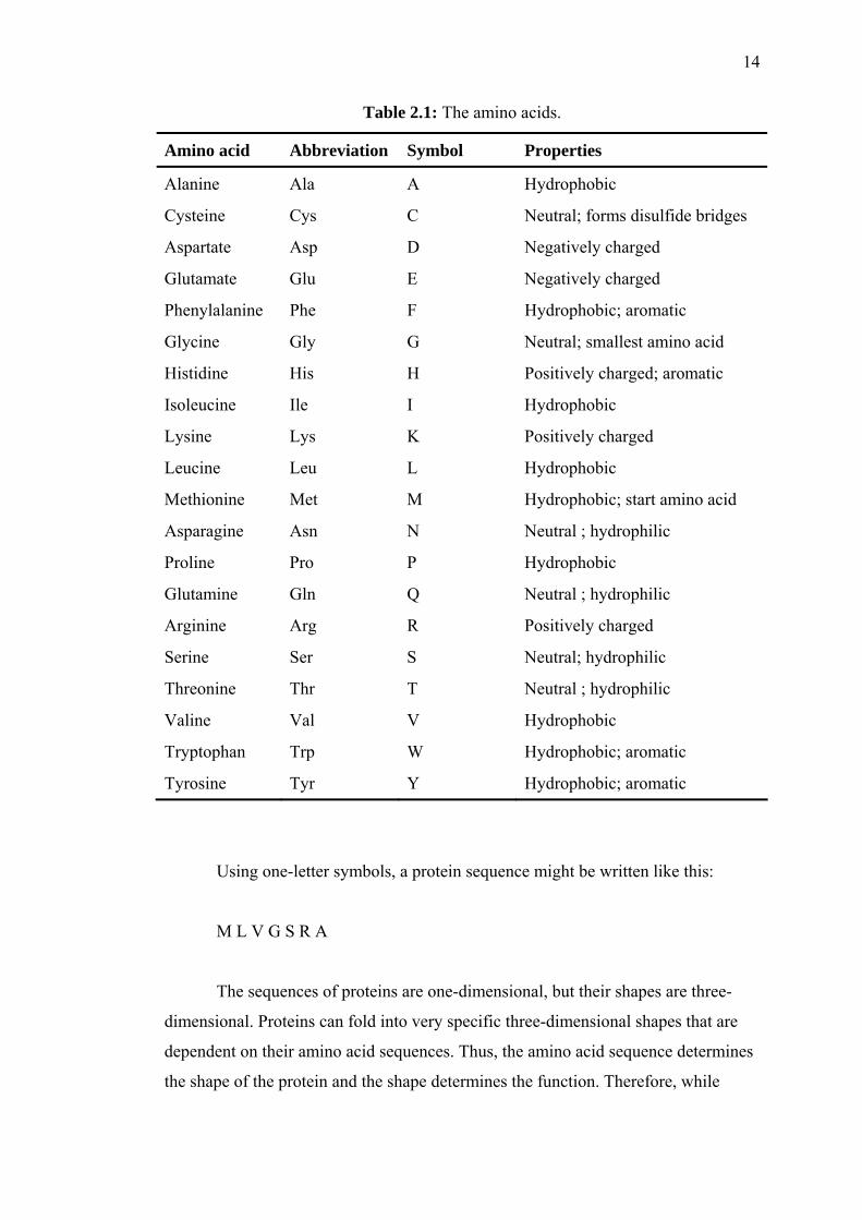
The protein alphabet contains 20 symbols, A, C, D, E, F, G, H, I, K, L, M, N,

P, Q, R, S, T, V, W, and Y. The names, abbreviations, and structures of the amino

acids are shown in Table 2.1.

14

Table 2.1: The amino acids.

Amino acid Abbreviation Symbol Properties

Alanine Ala A Hydrophobic

Cysteine Cys C Neutral; forms disulfide bridges

Aspartate Asp D Negatively charged

Glutamate Glu E Negatively charged

Phenylalanine Phe F Hydrophobic; aromatic

Glycine Gly G Neutral; smallest amino acid

Histidine His H Positively charged; aromatic

Isoleucine Ile I Hydrophobic

Lysine Lys K Positively charged

Leucine Leu L Hydrophobic

Methionine Met M Hydrophobic; start amino acid

Asparagine Asn N Neutral ; hydrophilic

Proline Pro P Hydrophobic

Glutamine Gln Q Neutral ; hydrophilic

Arginine Arg R Positively charged

Serine Ser S Neutral; hydrophilic

Threonine Thr T Neutral ; hydrophilic

Valine Val V Hydrophobic

Tryptophan Trp W Hydrophobic; aromatic

Tyrosine Tyr Y Hydrophobic; aromatic

Using one-letter symbols, a protein sequence might be written like this:

M L V G S R A

The sequences of proteins are one-dimensional, but their shapes are three-

dimensional. Proteins can fold into very specific three-dimensional shapes that are

dependent on their amino acid sequences. Thus, the amino acid sequence determines

the shape of the protein and the shape determines the function. Therefore, while

15

DNA and RNA are largely used to store and send information, proteins carry out

almost all processes in the cell. Also, proteins determine the shape and structure of

the cell, and also serve as the main instruments of molecular recognition and

catalysis.

Although proteins have many different shapes and sizes, if we look closely at

the structure, we can find recurring structural themes that biologists call secondary

structure. The most common themes are the α-helix, β-sheet, and random coil. In

Figure 2.2, these themes are represented as cylinders, arrows, and squiggly lines.

Figure 2.2: Schematic drawing of protein secondary structure (Punta et al., 2005).

When the sequences of primary structures tend to arrange themselves into

regular formations, these units are referred to as secondary structure. The angles and

hydrogen bond patterns between backbone atoms are determinant factors in protein

16

secondary structure. Secondary structure is subdivided into three parts: alpha-helix,

beta-sheet and loop.

Alpha-helix is spiral turns of amino acids while a beta-sheet is flat segments

or strands of amino acids formed usually by a series of hydrogen bonds. Beta-strands

are the most regular form of extended polypeptide chain in protein structures. Loops

usually serve as connection points between alpha-helices and beta-sheets. The do not

have patterns like alpha-helices and beta-sheets and they could be any other part of

the protein structure. They are sometimes known as random coil.

2.4 The Genetic Code

The information in DNA and RNA is translated to protein sequence using a

complex machine composed of proteins and ncRNAs called the ribosome reads an

mRNA sequence and writes a protein sequence. The mRNA is read three nucleotides

at a time. The nucleotide triplets are called codons. Each codon corresponds to a

single amino acid. The mapping from codons to amino acids is called the genetic

code. The genetic code is one of the universal laws of molecular biology.

Because codons are three nucleotides long and there are four possible

nucleotides at each position, it follows that there are 64 (43) possible codons.

However, there are only 20 amino acids. Therefore there is a redundancy in the

genetic code. Table 2.2 shows the standard nuclear genetic code. It can be observed

from Table 2.2 that there is a pattern in the genetic code redundancies. For example,

the third position of a codon is often insignificant; A, C, G, or T all lead to the same

translation. When this isn't the case, A and G are usually synonymous, as are C and

T. A and G belong to the same chemical class, called purines, and C and T belong to

another class, called pyrimidines. In addition to the amino acids, there are three stop

codons. When a ribosome catches a stop codon, translation terminates, and the

protein is released. All proteins start with the amino acid methionine. This has only

one codon, ATG, and so ATG is often called the start codon.

17

Table2.2: The standard genetic code.

Second Position

T C A G

T

TTT Phe (F)

TTC Phe (F)

TTA Leu (L)

TTG Leu (L)

TCT Ser (S)

TCC Ser (S)

TCA Ser (S)

TCG Ser (S)

TAT Tyr (Y)

TAC

TAA STOP

TAG STOP

TGT Cys (C)

TGC

TGA STOP

TGG Trp (W)

T

C

A

G

C

CTT Leu (L)

CTC Leu (L)

CTA Leu (L)

CTG Leu (L)

CCT Pro (P)

CCC Pro (P)

CCA Pro (P)

CCG Pro (P)

CAT His (H)

CAC His (H)

CAA Gln (Q)

CAG Gln (Q)

CGT Arg (R)

CGC Arg (R)

CGA Arg (R)

CGG Arg (R)

T

C

A

G

A

ATT Ile (I)

ATC Ile (I)

ATA Ile (I)

ATG Met (M)

ACT Thr (T)

ACC Thr (T)

ACA Thr (T)

ACG Thr (T)

AAT Asn (N)

AAC Asn (N)

AAA Lys (K)

AAG Lys (K)

AGT Ser (S)

AGC Ser (S)

AGA Arg (R)

AGG Arg (R)

T

C

A

G

F

i

r

s

t

P

o

s

i

t

i

o

n G

GTT Val (V)

GTC Val (V)

GTA Val (V)

GTG Val (V)

GCT Ala (A)

GCC Ala (A)

GCA Ala (A)

GCG Ala (A)

GAT Asp (D)

GAC Asp (D)

GAA Glu (E)

GAG Glu (E)

GGT Gly (G)

GGC Gly (G)

GGA Gly (G)

GGG Gly (G)

T

C

A

G

T

h

i

r

d

P

o

s

i

t

i

o

n

2.5 Proteins Functions

Proteins are the main players within the cell, known to be carrying out the

duties specified by the information encoded in genes (Lodish et al., 2004). Proteins

compose half the dry weight of a cell, while other macromolecules such as DNA and

RNA compose only 3% and 20% respectively (Voet and Voet, 2004). The total

18

complement of proteins expressed in a particular cell or cell type at a given time

point or experimental condition is known as its proteome.

The main characteristic of proteins that enables them to carry out their

diverse cellular functions is their ability to bind other molecules specifically and

tightly. The region of the protein responsible for binding another molecule is known

as the binding site and is often a depression or "pocket" on the molecular surface

(Lodish et al., 2004). This binding ability is mediated by the tertiary structure of the

protein, which defines the binding site pocket, and by the chemical properties of the

surrounding amino acids' side chains.

Proteins can bind to other proteins as well as to small-molecule substrates.

When proteins bind specifically to other copies of the same molecule, they can

oligomerize to form fibrils. Protein-protein interactions also regulate enzymatic

activity, control progression through the cell cycle, and allow the assembly of large

protein complexes that carry out many closely related reactions with a common

biological function. Proteins can also bind to, or even be integrated into, cell

membranes. The ability of binding partners to induce conformational changes in

proteins allows the construction of enormously complex signaling networks. Table

2.3 summarizes the different proteomic functions. The following paragraphs describe

some of these functions briefly.

Table 2.3: Proteins functions.

Protein Function Description Examples

Catalytic proteins

(Enzymes)

Catalyze reactions in cell Lactase

Protein kinase

RNase

Chymotrypsin

Regulatory proteins Modulate biological activity Insulin

DNA-binding proteins

Defense proteins Protect organism Immunoglobulins

Antibiotics

19

Transport proteins Bind and carry specific

molecules or ions

Hemoglobin

Structural Proteins Support or strengthen

biological structures

Collagen–tendon

Cartilage

Leather

Nutrient/Storage proteins Source of amino acids Ovalbumin–egg white

Casein–milk

The best-known function or role of proteins in the cell is their duty as

enzymes, which catalyze chemical reactions. Enzymes are usually highly specific

catalysts that accelerate only one or a few chemical reactions. Enzymes affect most

of the reactions involved in metabolism and catabolism as well as DNA replication,

DNA repair, and RNA synthesis. Some enzymes act on other proteins to add or

remove chemical groups in a process known as post-translational modification.

About 4,000 reactions are known to be catalyzed by enzymes (Bairoch, 2000).

Many proteins are involved in the process of cell signaling and signal

transduction. Some proteins, such as insulin, are extra-cellular proteins that transmit

a signal from the cell in which they were synthesized to other cells in distant tissues.

Others are membrane proteins that act as receptors whose main function is to bind a

signaling molecule and induce a biochemical response in the cell.

Antibodies are protein components of adaptive immune system whose main

function is to bind antigens, or foreign substances in the body, and target them for

destruction. Antibodies can be secreted into the extra-cellular environment or

anchored in the membranes of specialized B cells known as plasma cells. While

enzymes are limited in their binding affinity for their substrates by the necessity of

conducting their reaction, antibodies have no such constraints. An antibody's binding

affinity to its target is extraordinarily high.

20

Many ligand transport proteins bind particular small biomolecules and

transport them to other locations in the body of a multicellular organism. These

proteins must have a high binding affinity when their ligand is present in high

concentrations but must also release the ligand when it is present at low

concentrations in the target tissues. The canonical example of a ligand-binding

protein is haemoglobin, which transports oxygen from the lungs to other organs and

tissues in all vertebrates and has close homologs in every biological kingdom.

Structural proteins confer stiffness and rigidity to otherwise fluid biological

components. Most structural proteins are fibrous proteins; for example, actin and

tubulin are globular and soluble as monomers but polymerize to form long, stiff

fibers that comprise the cytoskeleton, which allows the cell to maintain its shape and

size. Collagen and elastin are critical components of connective tissue such as

cartilage, and keratin is found in hard or filamentous structures such as hair, nails,

feathers, hooves, and some animal shells.

2.6 Protein-Protein Interactions

Protein-protein interactions refer to the association of protein molecules and

the study of these associations from the perspective of biochemistry, signal

transduction and networks. Proteins might interact for a long time to form part of a

protein complex or a protein may interact briefly with another protein just to modify

it (for example, a protein kinase will add a phosphate to a target protein).

Protein-protein interactions are essential to virtually every cellular process

(Phizicky and Fields, 1995). For example, signals from the exterior of a cell are

mediated to the inside of that cell by protein-protein interactions of the signaling

molecules. This process, called signal transduction, plays a fundamental role in many

biological processes and in many diseases (e.g. cancer).

It has been proposed that all proteins in a given cell are connected in a huge

network in which certain protein interactions are forming and dissociating constantly

21

(Bork et al., 2004). An interaction map of the yeast proteome assembled from

published interactions is shown in Figure 2.3. The map contains 1,548 proteins

(boxes) and 2,358 interactions (connecting lines) (Schwikowski et al., 2000).

It is also estimated that even simple single-celled organisms such as yeast

have their roughly 6000 proteins interact by at least 3 interactions per protein, i.e. a

total of 20,000 interactions or more. By extrapolation, there may be on the order of

~100,000 interactions in the human body.

Figure 2.3: The protein-protein interaction network in yeast (Schwikowski et al.,

2000).

22

Any listing of major research topics in biology - for example, DNA

replication, transcription, translation, splicing, secretion, cell cycle control, signal

transduction, and intermediary metabolism - is also a listing of processes in which

protein complexes have been implicated as essential components (Phizicky and

Fields, 1995). Figure 2.4 shows Ribosomes or RNA polymerases as an example for

protein-protein interactions in a multi-protein complex. The schematic interaction

diagram for the 10 subunits in RNA polymerases complex is shown in Figure 2.4 (b).

(a) (b)

Figure 2.4: (a) Large protein complex and its protein-protein interactions.

(b) The schematic interaction (Cramer et al., 2001).

Protein-protein interactions can be classified based on the proteins involved

(structural or functional groups) or based on their physical properties (weak and

transient vs. strong and permanent). Protein interactions are usually mediated by

defined domains. Hence interactions can also be classified based on the underlying

domains.

Experimentally, interactions between pairs of proteins can be detected from

yeast two-hybrid systems, from affinity purification/mass spectrometry assays, or

from protein microarrays. In parallel to the experimental determination of the

protein-protein interactions, computational methods are being developed. Protein-

23

protein interaction prediction is a field combining computational techniques and

structural biology in an attempt to identify and catalog interactions between pairs or

groups of proteins.

Forces that mediate protein-protein interactions include electrostatic

interactions, hydrogen bonds, the van der Waals attraction and hydrophobic effects.

The average protein-protein interface is not less polar or more hydrophobic than the

surface remaining in contact with the solvent. Water is usually excluded from the

contact region. Non-obligate complexes tend to be more hydrophilic in comparison,

as each component has to exist independently in the cell.

It has been proposed that hydrophobic forces drive protein-protein

interactions and hydrogen bonds and salt bridges confer specificity (Young et al.,

1994). Van der Waals interactions occur between all neighbouring atoms, but these

interactions at the interface are no more energetically favorable than those made with

the solvent. However, they are more numerous, as the tightly packed interfaces are

denser than the solvent and hence they contribute to the binding energy of

association.

Hydrogen bonds between protein molecules are more favourable than those

made with water. Interfaces in permanent associations tend to have fewer hydrogen

bonds than interfaces in non-obligate associations. Interfaces have been shown to be

more hydrophobic than the exterior but less hydrophobic than the interior of a

protein. Permanent complexes have interfaces that contain hydrophobic residues,

whilst the interfaces in non-obligate complexes favour the more polar residues

(Koike and Takagi, 2003).

Most of the interactions data have been identified by high-throughput

technologies like the yeast two-hybrid system, which are known to yield many false

positives (Kim et al., 2002). In addition, in vivo experiments that identify protein-

protein interaction are still time-consuming and labor-intensive; besides, they

identify a small number of interactions. As a result, methods for computational

prediction of protein-protein interactions based on sequence information are

becoming increasingly important.

24

2.7 Summary

In this chapter, various concepts in molecular biology have been presented.

This is essential to facilitate better understanding of the research discussed in this

thesis. In conclusion, protein-protein interactions are of central importance for

virtually every process in a living cell. Information about these interactions improves

our understanding of diseases and can provide the basis for new therapeutic

approaches.

CHAPTER 3

LITERATURE REVIEW

Related research in the field of computational prediction of protein-protein

interactions is presented in this chapter. This chapter begins by reviewing several

approaches to protein function prediction and its relation to protein-protein

interactions. After that it describes the experimental techniques that are being used to

determine and identify protein-protein interactions and highlights the need for

computational approaches. Then it reviews the research that has been done to

computationally predict protein-protein interactions. At the end, a summary of the

literature review is presented.

3.1 Protein Function Prediction

The field of bioinformatics has arisen in parallel with the development of

automated high throughput methods of biological and biochemical discovery that

yield a variety of forms of experimental data, such as DNA sequences, gene

expression patterns, and chemical structures. One of the major challenging tasks in

bioinformatics is to infer and predict the function of the newly discovered proteins.

Proteins carry out the majority of tasks in organisms, such as catalysis of

biochemical reactions, transport of nutrients, recognition and transmission of signals.

The role of any particular protein is referred to as its function. However, protein

function is not a well-defined term; instead function is a complex phenomenon that is

26

associated with many mutually overlapping levels: biochemical, cellular, organism

mediated, developmental, and physiological. Thus, the determination of protein

functions is a complex problem in bioinformatics research. The sequencing of entire

genomes has moved the attention from the study of single proteins or small

complexes to that of the entire proteome (Hodgman, 2000).

One of the most fundamental tools in the field of bioinformatics is sequence

alignment. By aligning sequences to one another, it is possible to evaluate how

similar the sequences are and identify conserved regions in sets of related sequences.

This is used extensively to assign function to genes in newly sequenced genomes.

Although, most methods annotating protein function utilise sequence homology to

proteins of experimentally known function, such a homology-based annotation

transfer is problematic and limited in scope. Therefore, researchers have begun to

develop different methods that predict protein function, including phylogenetic

patterns, gene expression, and protein-protein interactions. Figure 3.1 shows different

approaches to infer and predict protein function.

Protein Sequence

Protein Structure

Wet Lab

Protein Interactions

Protein Homology

Protein Function

Phylogenetic patterns

Gene expression

Figure 3.1: Different methods for inferring protein function.

27

The Yeast Protein Database (YPD) lists 6281 proteins with 3854 being

annotated, assigned to some cellular roles, and 2427 being unannotated (Costanzo et

al., 2001). A challenging task that lies ahead is to find the functional roles of these

unannotated proteins. Several research groups have developed methods for

functional annotation. The classical way is to find homologies between a protein and

other proteins in protein databases using programs such as FASTA (Pearson, 2000)

and PSI-BLAST (Altschul et al., 1997), and then predict functions based on

sequence homologies. Besides, functional predictions have been modeled as pattern

recognition problems based on sequence homologies and structural information

(King et al., 2001) as well as phenotype data (Clare and King, 2002).

When function cannot be inferred based on sequences similarity, one must

rely on true ab initio prediction methods. It is a generally accepted paradigm that the

function of a protein is determined by its three-dimensional structure, and that the

structure is determined by the sequence of the protein. Given this paradigm, it would

be logical to think that ab initio function prediction could be done by first predicting

the structure of the protein, and subsequently predict the function from the structure.

However, both steps in this approach are likely to be very difficult to solve.

Knowing the structure of a protein does not mean that it is necessarily

possible to figure out what the protein does, even though it is of course a big help

(Norin and Sundstrom, 2002). This is because the function of a protein depends on

its cellular context. Also, post-translational modifications can profoundly alter the

function (and structure) of a protein. Predicting the function of a protein from its

structure may therefore very well turn out to be as difficult as the protein folding

problem.

However, since proteins collaborate or interact with one another for a

common purpose, it is possible to deduce functions of a protein through the functions

of its interaction partners (Deng et al.,2002; Letovsky and Kasif, 2003). The protein-

protein interaction network describes a neighborhood structure among the proteins. If

two proteins interact, they are neighbors of each others. For an unannotated protein,

the functions of its neighbors can tell us something about the function of the

28

unannotated protein. For a given function, if most of the neighbors of a protein have

the function, it is more likely to be believed that the protein have the same function.

It should be noted that the interaction partners for a protein may belong to

different functional categories. It is this complex network of within function and

cross-function interactions that makes the problem of functional assignments a

difficult task. Methods based on frequencies of interaction partners having certain

functions of interest (Schwikowski et al., 2000) and on χ2-statistics (Hishigaki et al.,

2001) have been applied to assign functions to unannotated proteins.

Schwikowski et al. (2000) proposed to infer the functions of an unannotated

protein based on the frequencies of its neighbors having certain functions. They

assign k functions to the unannotated protein with the k largest frequencies in its

neighbors. This approach will be referred as the neighboring counting method. This

approach does not consider the frequency of the proteins having a function among all

the proteins. If a function is more common than other functions among all the

proteins, the probability that an unannotated protein has this function should be

higher than the probability that it has other functions even if the protein does not

have interaction partners.

Hishigaki et al. (2001) developed another method to infer protein functions

based on χ2-statistics. For a protein Pi, let ni(j) be the number of proteins interacting

with Pi and having function Fj . Let ei(j) = #Nei(i) × πj be the expected number of

proteins in Nei(i) having function Fj , where #Nei(i) is the number of proteins in

Nei(i). Define

.)(

))()(()(

2

jejejn

jSi

iii

−=

(3.1)

For a fixed k, they assign an unannotated protein with k functions having the

top k χ2-statistics. Although this approach takes the frequency of the proteins having

a function into consideration, ni(j) is generally small and the applicability of the χ2-

statistics is questionable.

29

Another approach has been developed by Deng et al. (2002) in which they

apply the theory of Markov random fields to infer a protein’s functions using protein-

protein interaction data and the functional annotations of its interaction protein

partners. For each function of interest and a protein, they predict the probability that

the protein has that function using Bayesian approaches. Unlike in other available

approaches for protein annotation where a protein has or does not have a function of

interest, they give a probability for having the function. This probability indicates

how certain it can be believed about the prediction.

Recently, Letovsky and Kasif (2003) applied a method of assigning functions

based on a probabilistic analysis of graph neighborhoods in a protein-protein

interaction network. The method exploits the fact that graph neighbors are more

likely to share functions than nodes which are not neighbors. A binomial model of

local neighbor function labeling probability is combined with a Markov random field

propagation algorithm to assign function probabilities for proteins in the network.

The method has been applied on a protein-protein interaction dataset for the yeast

Saccharomyces cerevisiae using the Gene Ontology (GO) terms as function labels.

The method reconstructed known GO term assignments with high precision, and

produced putative GO assignments to 320 proteins that currently lack GO annotation,

which represents about 10% of the unlabeled proteins in Saccharomyces cerevisiae.

Part of the reason why it is difficult to relate the chemical function of a

protein to its biological purpose is that proteins do not function alone. To understand

the function of a protein, it must be considered in its proper cellular context, for

example by appreciating how the cell would behave without it (Attwood and Miller,

2001). Many proteins are parts of larger complexes, which are the functional units

that fulfill a role in the cell (Gavin et al., 2002). In this case it can be argued that all

the proteins that form the complex should also have the same function. Since a

protein does not perform its function alone but in the context of many other proteins

as well as other biomolecules, it is highly relevant to study the interaction partners of

a protein in order to understand its function (Eisenberg et al., 2000; Ho et al., 2002).

30

The previous approaches to infer the unknown function of a class of proteins

have exploited sequence similarities or clustering of co-regulated genes (Harrington

et al., 2000), phylogenetic profiles (Pellegrini et al.,1999), protein-protein

interactions (Uetz et al., 2000; Ito et al., 2000; Schwikowski et al.,2000; Deng et al.,

2002), and protein complexes (Gavin et al., 2002; Ho et al., 2002). Table 3.1

summarizes different approaches and techniques to infer and predict protein function.

Table 3.1: Computational methods for protein function prediction.

Approach Technique Researches FASTA Pearson, 2000 Sequence alignments PSI-BLAST Altschul et al., 1997 BLOCKS Henikoff & Henikoff, 1994 PRINTS Attwood et al., 1997

Multiple sequence alignments

PRODOM Sonnhammer & kahn, 1994 Hidden Markove Models Karplus et al., 1997 Protein structure

prediction Nearest-neighbor algorithms Salamov & Solovyev 1995 Phylogenetic patterns

Statistical methods Pellegrini et al., 1999

SVM Brown et al., 2000 Gene expression data analysis Statistical algorithm Eisen et al., 1998 Family Identification

Normalized cuts clustering algorithm

Abascal & Valencia, 2003

n-neighbouring proteins Hishigaki et al., 2001 Markov random fields and Bayesian networks

Deng et al., 2002

Global optimization and simulated annealing

Vazquez et al., 2003

Protein-protein interaction

Markov random fields and label propagation algorithm

Letovsky & Kasif 2003

3.2 Methods to study protein-protein interactions

Protein-protein interactions are working at almost every level of cell function,

in the structure of sub-cellular organelles, the transport machinery across the various

biological membranes, packaging of chromatin, the network of sub-membrane

filaments, muscle contraction, and signal transduction, regulation of gene expression,

to name a few (Donaldson et al., 2003) . Abnormal protein-protein interactions have

31

implications in a number of neurological disorders such as Creutzfeld-Jacob and

Alzheimer's disease.

Because of their importance in cell development and disease, protein-protein

interactions have gained a lot of attention among researchers for many years. It has

emerged from these studies that there is a strategy of mixing and matching of

domains that specify particular classes of protein-protein interactions. There are a

large number of methods to detect protein-protein interactions. Each of the

approaches has its own strengths and weaknesses, especially with regard to the

sensitivity and specificity of the method. A high sensitivity means that many of the

interactions that occur in reality are detected by the method. A high specificity

indicates that most of the interactions detected by the screen are also occurring in

reality.

Co-immunoprecipitation is considered to be the gold standard assay for

protein-protein interactions, especially when it is performed with endogenous (not

overexpressed and not tagged) proteins (Gharakhanian et al., 1988). The protein of

interest is isolated with a specific antibody. Interaction partners which stick to this

protein are subsequently identified by western blotting. Interactions detected by this

approach are considered to be real. However, this method can only verify

interactions between suspected interaction partners. Thus, it is not a screening

approach to identify unknown protein-protein interactions.

The yeast two-hybrid screen investigates the interaction between artificial

fusion proteins inside the nucleus of yeast (Bartel and Fields, 1997). This approach

can identify binding partners of a protein in an unbiased manner. However, this

method suffers from high false-positive rate which makes it necessary to verify the

identified interactions by co-immunoprecipitation.

Tandem affinity purification (TAP) detects interactions within the correct

cellular environment (e.g. in the cytosol of a mammalian cell) (Rigaut et al., 1999).

This is a big advantage compared to the yeast two-hybrid approach. However, the

TAP tag method requires two successive steps of protein purification. Thus, it can

not readily detect transient protein-protein interactions. It is also not efficient to

32

detect physical protein-protein interactions that exist in different cellular

environment. This is especially important when studying the interaction network in

the organism’s genome which becomes very significant in the post-genomic era.

Quantitative immunoprecipitation combined with knock-down (QUICK)

relies on co-immunoprecipitation, quantitative mass spectrometry (SILAC) and RNA

interference (RNAi). This method detects interactions among endogenous non-

tagged proteins (Selbach and Mann, 2006). Thus, it has the same high confidence as

co-immunoprecipitation. However, this method also depends on the availability of

suitable antibodies.

Dual Polarisation Interferometry (DPI) is a method that can be used to

measure protein-protein interactions. DPI provides real-time, high-resolution

measurements of molecular size, density and mass. However this method can not be

used to detect new protein-protein interactions.

3.3 Predicting Protein-Protein Interactions

Protein-protein interactions play a crucial role in protein function. Hence, the

ability to computationally recognize protein interaction sites and to identify specific

interface residues that contribute to the specificity and affinity of protein interactions

has important implications in a wide range of clinical and industrial applications.

Until recently, information about protein–protein interactions was gathered

via experiments that were individually designed to identify and validate a small

number of specifically targeted interactions. This traditional source of information

has been augmented recently by the results of high-throughput experiments designed

to exhaustively probe all the potential interactions within entire genomes (Table 3.2).

However, the many discrepancies between the interacting partners identified in high-

throughput studies and those identified in small scale experiments highlight the need

for caution when interpreting results from high-throughput studies.

33

Table 3.2: High-throughput experimental approaches to the determination of

protein-protein interactions.

Method References Features

Uetz et al., 2000

Ito et al., 2000

Newman et al., 2000

The first comprehensive studies in yeast

Boulton et al., 2002

Yeast two-hybrid

Walhout et al., 2002

Combined analysis of yeast two-hybrid interactions together with phenotype and expression data

Affinity purification/mass

Ho et al., 2002 Purification of overexpressed, epitope-tagged proteins in yeast

spectrometric identification

Gavin et al., 2002 TAP purification of complexes expressed at physiological levels in yeast

Protein chips Zhu et al., 2001 High-throughput detection of interactions with proteins over-expressed and immobilized on microscope slides to form a proteome microarray

Synthetic lethals Tong et al., 2001 High-throughput identification of synthetic lethal double mutants. Synthetic lethal mutants often correspond to physically interacting protein pairs.

Phage display Tong et al., 2002 Phage display identification of binding motifs followed by computational identification of potential interacting partners and a yeast two-hybrid validation step

34

High-throughput experimental techniques enable the study of protein-protein

interactions at the proteome scale through systematic identification of physical

interactions among all proteins in an organism. High-throughput protein-protein

interaction data, with ever-increasing volume, are becoming the foundation for new

biological discoveries.

A great challenge to bioinformatics is to manage, analyze, and model these

data. Comparison between experimental techniques shows that each high-throughput

technique such as yeast two-hybrid assay or protein complex identification through

mass spectrometry has its limitations in detecting certain types of interactions and

they are complementary to each other. Moreover the overlap between these high-

throughput experiments is very small as shown in Figure 3.2.

Figure 3.2: The overlap between different high-throughput experiments.

The limitations of the experimental methods to identify protein-protein

interactions highlight the need for computational methods to infer and predict

protein-protein interactions. As a result, complementary computationally methods

capable of accurately predicting interactions would be of considerable value.

Furthermore, computational methods for the prediction of protein interactions will

provide more data which will enable predicting protein function more precisely since

35

the function of proteins with three or more partners can be more accurately predicted

than with information about one partner.

It is also important to note that computational methods that use protein

sequences, domain and structure information to predict protein-protein interaction

can expand the scope of experimental data and increase the confidence of certain

protein-protein interaction pairs.

Protein-protein interaction data correlate with other types of data, including

protein function, subcellular location, and gene expression profile. Highly connected

proteins are more likely to be essential based on the analyses of the global

architecture of large-scale interaction network in yeast. The use of protein-protein

interaction networks, preferably in conjunction with other types of data, allows

assignment of cellular functions to novel proteins and derivation of new biological

pathways.

Several approaches have been proposed for predicting protein-protein

interaction sites from amino acid sequence or from a combination of sequence and

structural information (see Table 3.3.). For example, based on their observation that

proline residues occur frequently near interaction sites, Kini and Evans (1996)

predicted potential protein-protein interaction sites by detecting the presence of

"proline brackets." Building on their systematic patch analysis of interaction sites,

Jones and Thornton (1997) successfully predicted interfaces in a set of 59 structures

using a scoring function based on six parameters. Gallet et al. (2000) identified

interacting residues using an analysis of sequence hydrophobicity based on a method

previously developed by Eisenberg et al. (1984) for detecting membrane and surface

segments of proteins.

36

Table 3.3: Computational methods for protein-protein interactions prediction.

Approach Technique References

Identifying interacting sequence motif pairs.

Statistical Method Wojcik & Schachter, 2001

Co-occurrence of sequence domains.

Probabilistic model Deng et al., 2002

Gene fusion Rosetta stone Marcotte et al., 2000

Threading-based interaction energy evaluation.

Statistical methods Lu et al., 2002

Phylogenetic profile method.

Statistical methods Pellegrini et al., 1999

Craig and Liao, 2007

Gene Ontology Semantic similarity search

Wu et al., 2006

Ofran & Rost, 2003 SVM

Koike & Takagi, 2003

Identification of Surface residues

Statistical Method Gallet et al., 2000

Bock & Gough, 2001

Dohkan et al., 2003

Ben-Hur & Noble, 2005

SVM

Dohkan et al., 2006

SVM + Attraction-repulsion model

Gomez et al., 2003

Bayesian Networks Jansen et al., 2003

Lin et al., 2004

Primary structure based prediction

Set Cover Approach Huang et al., 2007

37

Prediction of interaction sites in proteins of known structure usually focuses

on the location of hydrophobic surface clusters on proteins. In one study, this method

predicted the correct interaction site in 25 out of 29 cases (Zhou and Shan, 2001).

Other methods include solvation potential, residue interface propensity,

hydrophobicity, planarity, protrusion, and accessible surface area. Among a test set

of 28 homodimers, the known interface site was found to be amongst the most

planar, protruding, and accessible patches, and amongst the patches with highest

interface propensity. Nevertheless, one of the algorithms (PATCH) that uses multiple

parameters predicted the location of interface sites in known complexes only for 66%

of the structures.

Based on the idea that domains mediate the interactions between proteins, Ng

et al. (2003) collected data from three data sources to develop the database of

interacting domains (InterDom). The first one is the experimentally derived protein

interaction data from the Database of Interacting Proteins (DIP) (Xenarios et al.,

2002). The second source is the intermolecular relationship data from protein

complexes and the last one is the computationally predicted data from Rosetta Stone

sequences. Then they infer putative domain-domain interaction based on the

collected data. This is very helpful when inferring protein-protein interactions for

proteins partners that have domain structure.

Another approach is to predict protein-protein interactions from genome

sequences. Several attempts have been made to achieve that. The major methods are:

• Rosetta stone proteins: Some protein sequences have been found to be

split into two independent proteins in other organisms. From such

sequences it has been concluded that the two independent proteins form

a complex, based on the (covalent) association in the former organism.

Such fusion proteins are called Rosetta stone proteins (Edward et al.,

1999). Supposedly they predict interactions among related proteins.

Example: human succinyl CoA transferase is split in E. coli into acetate

CoA transferases alfa and beta subunits.

38

• Phylogenetic profiles: Some protein pairs are evolutionarily maintained

together in many different organisms. It has been concluded that such

“co-evolving” proteins are associated either functionally or even

physically, i.e. by a protein-protein interactions (Marcotte et al., 2000).

While the latter is not always true, it has been found to be true in a

number of cases, such as the yeast proteins Hog1 and Fus3. Also the

phylogenetic species tree of the reference genomes can be used as a

guide tree for hierarchical clustering of the orthologous proteins (Craig

and Liao, 2007). They have shown that the phylogenetic tree can be

used as a guide to extract intra-matrix correlations in the distance

matrices of orthologous proteins, where these correlations are

represented as intermediate distance matrices of the ancestral

orthologous proteins.

By measuring the similarity between two Gene Ontology (GO) terms with a

relative specificity semantic relation, Wu et al., (2006) proposed a method of

reconstructing a yeast protein–protein interaction map that is solely based on the GO

annotations. The method was validated using high-quality interaction datasets for its

effectiveness. Based on a Z-score analysis, a positive dataset and a negative dataset

for protein–protein interactions were derived. This analysis could be efficient on

predicting functional protein-protein interactions based on the GO terms similarity.

However, it could suffer from high rate of false positive since many protein share

similar function but are not physically interacting.

In addition to the above methods for predicting protein-protein interactions

from genome sequence, machine learning methods have been recently applied. It is

based on the idea that a pattern of interactions can be learned from the available

protein-protein interactions data. Using machine learning methods and techniques

could be very useful in terms of producing vast amount of possible protein-protein

interactions. It could also assist the biologists in pursuing for further analysis on the

potential interactions.

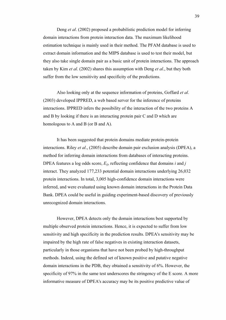
39

Deng et al. (2002) proposed a probabilistic prediction model for inferring

domain interactions from protein interaction data. The maximum likelihood

estimation technique is mainly used in their method. The PFAM database is used to

extract domain information and the MIPS database is used to test their model, but

they also take single domain pair as a basic unit of protein interactions. The approach

taken by Kim et al. (2002) shares this assumption with Deng et al., but they both

suffer from the low sensitivity and specificity of the predictions.

Also looking only at the sequence information of proteins, Goffard et al.

(2003) developed IPPRED, a web based server for the inference of proteins

interactions. IPPRED infers the possibility of the interaction of the two proteins A

and B by looking if there is an interacting protein pair C and D which are

homologous to A and B (or B and A).

It has been suggested that protein domains mediate protein-protein

interactions. Riley et al., (2005) describe domain pair exclusion analysis (DPEA), a

method for inferring domain interactions from databases of interacting proteins.

DPEA features a log odds score, Eij, reflecting confidence that domains i and j

interact. They analyzed 177,233 potential domain interactions underlying 26,032

protein interactions. In total, 3,005 high-confidence domain interactions were

inferred, and were evaluated using known domain interactions in the Protein Data

Bank. DPEA could be useful in guiding experiment-based discovery of previously

unrecognized domain interactions.

However, DPEA detects only the domain interactions best supported by

multiple observed protein interactions. Hence, it is expected to suffer from low

sensitivity and high specificity in the prediction results. DPEA's sensitivity may be

impaired by the high rate of false negatives in existing interaction datasets,

particularly in those organisms that have not been probed by high-throughput

methods. Indeed, using the defined set of known positive and putative negative

domain interactions in the PDB, they obtained a sensitivity of 6%. However, the

specificity of 97% in the same test underscores the stringency of the E score. A more

informative measure of DPEA's accuracy may be its positive predictive value of

40

70%, implying that roughly 2/3 of the high-confidence domain interactions inferred

by DPEA are true positives; the remaining 1/3 are likely false positives.

Based on the currently available protein-protein interaction and domain data,

(Huang et al., 2007) described Maximum Specificity Set Cover (MSSC) method for

the prediction of protein-protein interactions. In this approach, they mapped the

relationship between interactions of proteins and their corresponding domain

architectures to a generalized weighted set cover problem. The application of a

greedy algorithm provides sets of domain interactions which explain the presence of

protein interactions to the largest degree of specificity.

Utilizing domain and protein interaction data of S. cerevisiae, MSSC enables

prediction of previously unknown protein interactions, links that are well supported

by a high tendency of coexpression and functional homogeneity of the corresponding

proteins. Focusing on concrete examples, they showed that MSSC reliably predicts

protein interactions in well-studied molecular systems, such as the 26S proteasome

and RNA polymerase II of S. cerevisiae.

However, MSSC algorithm only allows predictions between proteins with

well-known domain structure as well as known interactions among the respective

domains. In this approach, other sequence information is not included but only

inferring potential domain interactions by counting the occurrence of all possible

domain pairs that the domain structure of interacting proteins. This implies a method

that risks an elevated level of noise in the determination of potential domain

interactions. Accordingly, the error proneness of protein interactions in the respective

training sets is another source of potential noise, impacting the quality of predictions.

In addition to these approaches, several different methods that rely on

multiple sequence alignment and exploit conserved residues or correlated mutations

to detect protein-protein interaction sites have been proposed (Lichtarge et al., 1996;

Pazos et al., 1997). More recently, methods using a support vector machine (SVM)

based on primary sequence and associated physicochemical properties have been

developed to predict protein-protein interactions (Bock and Gough, 2001; Dohkan et

41

al., 2003). The use of SVM for predicting protein-protein interactions will be

discussed in the next section.

3.4 Support Vector Machines

The Support Vector Machine (SVM) is a binary classification algorithm. As

such it is well suited for the task of discriminating between interacting and non-

interacting protein pairs. SVMs have demonstrated high classification ability in the

field of prediction of protein-protein interaction, functional classification of proteins,

protein fold recognition, and prediction of subcellular location. SVMs have

previously been used in the prediction of protein-protein interaction (Bock and

Gough, 2001) (Dohkan et al., 2003) (Koike et al., 2003) (Chung et al., 2004).

The SVM is based on the idea of constructing the maximal margin

hyperplane in the feature space (Vapnik, 1995). Suppose we have a set of labeled

training data {xi, yi}, i = 1,…, n, yi∈{1,-1}, xi ∈ Rd, and have the separating

hyperplane (w . x) + b = 0, where feature vector: x ∈ Rd, w∈ Rd and b∈ R. In the

linear separable case the SVM simply looks for the separating hyperplane that

maximizes the margin by minimizing ||w||2/2 subject to the following constraint:

yi(w . xi + b) ≥ 1 ∀i (2.2)

In the linear non-separable case, the optimal separating hyperplane can be

found by introducing slack variables ξi, i = 1,…, n and user-adjustable parameter C

and then minimizing ||w||2/ 2 + C Σi ξi , subject to the following constraints:

yi(w . xi + b) ≥ 1 - ξi

ξi ≥ 0 ∀ (2.3) .,...,1 ni =

The dual optimization is solved here by introducing the Lagrange multipliers

αi for the non-separable case. Because linear function classes are not sufficient in

42

many cases, we can substitute Φ(xi) for each example xi and use the kernel function

K(xi,xj) such that Φ(xi).Φ(xj). We thus get the following optimization problem:

),(21max

1,1jijij

n

jii

n

ii xxKyyααα

α ∑∑==

− (2.4)

subject to ,0 Ci ≤≤α .,...,1 ni =

and (2.5) 01

=∑=

i

n

ii yα

SVM has the following advantages to process biological data (Bock and

Gough, 2001): (1) SVM is computationally efficient and it is characterized by fast

training which is essential for high-throughput screening of large protein datasets. (2)

SVM is readily adaptable to new data, allowing for continuous model updates in

parallel with the continuing growth of biological databases. (3) SVM provides a

principled means to estimate generalization performance via an analytic upper bound

on the generalization error. This means that a confidence level may be assigned to

the prediction, and avoids problems with overfitting inherent in neural network

function approximation.

Recently, SVM has been used to predict protein-protein interactions. For

example, Bock and Gough (2001) used SVM and physicochemical properties of

residues such as hydrophobicity and surface tension to predict protein-protein

interactions. The prediction methodology reported in their paper generates a binary

decision about potential protein–protein interactions, based only on primary structure

and associated physicochemical properties. Their results suggest the possibility of

proceeding directly from the automated identification of a cell’s gene products to

inference of the protein interaction pairs, facilitating protein function and cellular

signaling pathway identification. As they mention in their paper, their research

represents only an initial step in the automated prediction of protein interactions.

With experimental validation, further development along these lines may produce a

robust computational screening technique that narrows the range of putative

43

candidate proteins to those exceeding a prescribed threshold probability of

interaction.

In a recent paper, Dohkan et al. (2003) have proposed a new method to

predict protein-protein interactions using Support Vector Machines. In their method,

multiple domain effects and the physicochemical features can be considered all at

once. They mentioned that the prediction accuracy was clearly improved by adding

protein features such as amino acid composition and/or localization. Furthermore,

consideration of combined features domain, amino acid composition, and subcellular

localization resulted in the best prediction performance: an F-measure of 79%. The

present predictions seem to be more accurate than those reported previously.

Moreover they applied their method to the unknown protein pairs, and fount

that high scoring protein pairs were likely to have similar GO annotations. These

results indicate that the present method is useful inferring likely interactions between

unknown protein pairs and/or detect reliable protein interaction from high-throughput

data. Further, the similar GO annotation tendencies indicate the possibility of that the

biological function may be predicted by the prediction of protein interaction pairs.

They also evaluated the effects of using only the physicochemical features on the

prediction of protein-protein interactions. They retrained the SVM without using

domain information. The results imply that only the use of these physicochemical

properties is not sufficient to predict interactions accurately, and domain information

is quite informative.

3.5 Bayesian Networks

A Bayesian Network (BN) is a graphical model that encodes probabilistic

relationships among variables of interest. When used in conjunction with statistical

techniques, the graphical model has several advantages for data analysis (Jensen,

1996). One, because the model encodes dependencies among all variables, it readily

handles situations where some data entries are missing. Two, a Bayesian network can

be used to learn causal relationships, and hence can be used to gain understanding

44

about a problem domain and to predict the consequences of intervention. Three,

because the model has both a causal and probabilistic semantics, it is an ideal

representation for combining prior knowledge (which often comes in causal form)

and data. Four, Bayesian statistical methods in conjunction with Bayesian networks

offer an efficient and principled approach for avoiding the over fitting of data.

Given a set of variables D = {X1, X2…XN}, where each variable Xi could take

values from a set Val(Xi), a Bayesian Network describes the probability distribution

over this set of variables. The capital letters as X,Y are used to denote variables and

lower case letters as x,y to denote values taken by these variables. Formally, a BN is

an annotated directed acyclic graph (DAG) that encodes a joint probability

distribution. A network B can be denoted as a pair B = <G, Θ>, where G is a DAG

whose nodes symbolize the variables of D, and Θ refers to the set of parameters that

quantifies the network. G embeds the following conditional independence

assumption:

Each variable Xi is independent of its non-descendants given its parents.

Θ includes information about the probability distribution of a value xi of a

variable Xi, given the values of its immediate predecessors. The unique joint

probability distribution over {X1, X2…XN} that a network B describes can be

computed using:

))(|()...(1

1 ∏=

=N

iiiNB XparentsxPXXP (2.6)

Since large-scale data sets of protein interactions can be very noisy and can

lead to inaccuracies when trying to identify protein interactions on a genome-wide

scale and the data in the literature can be incomplete and contradictory, the Bayesian

Networks can be considered as a candidate approach to cope with this problem.

Jansen et al. (2003) have developed a Bayesian approach for integrating

weakly predictive genomic features into reliable predictions of protein-protein

interactions. They constructed protein interaction network for the yeast genome. In

45

this network, they combined four large-scale, highthroughput data sets of protein

interactions from the literature. This network is known as probabilistic interactome

experimental (PIE).

PIE is simply taking the existing but noisy interaction data sets and trying to

integrate them to create an optimal experimental interactome. In constructing the

network, each source of information is assessed by comparing it against a set of

“gold standards” of known positive and negative protein interactions. The positives

are taken from the Munich Information Center for Protein Sequences catalog of

known protein complexes. The negative protein interactions include proteins that are

known to be separated in different subcellular compartments. When the network is

compared to the gold standards, the predicted network turns out to be more accurate

than the existing experimental data sets. One of the main achievements of their

research is to predict protein interactions to a well-defined level of accuracy from

non-interaction information and show that these predictions are essentially as

accurate, if not more accurate, as directly getting the highthroughput interaction data.

Another research group has conducted an assessment study based on the

genomic features used in a Bayesian network, random forest and logistic regression

to predict protein-protein interactions genome-wide in yeast (Lin et al., 2004). The

non-Bayesian methods do not require prior information needed for the Bayesian

approach, and can fully utilize the raw data without discretization. They reported that

the logistic model performs similarly as the Bayesian method in terms of

classifications and, like the Bayesian method, produces estimated probabilities that

two proteins interact. As a dichotomous classifier, the random forest method

outperforms the other methods considered and efficiently uses the information,

although it is computationally more expensive. In particular, its importance measure

provides a more objective assessment of different genomic features on predicting

protein-protein interactions than simply considering contributions to model fitting.

46

3.6 Summary

This chapter has discussed the literature in the field of protein function

prediction problem. It has showed that it is possible to infer and protein function

from protein-protein interactions data. Many researchers have used the available

experimental data of protein-protein interactions to infer and predict protein function

of the unannotated proteins. However, according to the literature, the experimental

data is suffering from many false positive and has many discrepancies between

different experiments results. In the meantime there are many research have been

proposed to predict the protein-protein interaction using computational methods from

protein primary structure and associated features. Therefore, it would possible to

combine and validate the computationally predicted and the experimental protein

interactions data to construct more reliable dataset for predicting proteins function.

Hence, this research focuses on predicting protein-protein interactions from protein

sequence information using the support vector machines and Bayesian approach.

CHAPTER 4

THE RESEARCH METHODOLOGY

Based on the literature review discussed in Chapter 3, the main requirement is

to develop a machine learning technique that is capable to infer and predict protein-

protein interactions data. Basically, this chapter describes the research methodology

needed to fulfill the research objective. The datasets that is used in the experiments

of this research is presented and discussed as well as the evaluation measures of the

system performance are also discussed. In addition to the methodology, the expected

outcome at each stage of the investigation will be presented as well. At the end of

this chapter the assumptions and the limitations of this research will be presented.

4.1 Research Design

This research is an applied, scientific research using the problem oriented

approach. It involves several important issues: protein-protein interactions, Support

Vector Machines and Bayesian Methods. In this work, a machine learning method

based on a support vector machine (SVM) combined with a kernel function was

developed for the prediction of protein-protein interactions based only on the primary

sequences of proteins. The general research framework is presented in the next

section.

48

4.2 General Research Framework

Applying the conventional methods of machine learning approaches

including support vector machines without augmentation, to biological data bases

does not achieve good performance. This is due to the nature of the biological data

which is dynamic rather than static data conventionally used in patter recognition

problem solving. In this research, examining and studying different protein sequence

feature is carried out in order to identify the best feature that can be used to

accurately predict protein-protein interactions from protein sequences information.

Including biological information represented in the feature selection is essential for

successful machine learning approach.

Hence, this research framework is initiated by studying and comparing

different sequence features for the prediction of protein-protein interactions using the

support vector machines. Positive and negative datasets are required for training the

support vector machines. Although, constructing a positive dataset (i.e. pairs of

interacting proteins) is relatively an easy task by using one of the available databases

of interacting proteins, there is no data on experimentally confirmed non-interacting

protein pairs have been made available. To cope with this problem, some researchers

created an artificial negative protein interaction dataset for Saccharomyces cerevisiae

by randomly generating protein pairs from this organism that are not described as

interacting in the Database of Interacting Proteins (DIP) without putting any further

restrictions on such pairs, as in (Deane et al., 2002; Chung et al., 2004).

One problem with this approach is that in many cases selected non-interacting

protein pairs will possess features that are substantially different from those typically

found in the positive interaction set. This effect may simplify the learning task and

artificially raise classification accuracy for training data. There is no guarantee,

however, that the generalized classification accuracy will not degrade if the predictor

is presented with new, previously unseen data which are hard to classify. However,

this approach could be used for comparing different features or algorithms since the

error will be uniform among all features or algorithms.

49

Due to the unavailability of experimentally confirmed non-interacting

protein pairs, the problem of predicting protein-protein interactions is essentially

one-class classification problem. Accordingly, the One-Class SVM is proposed in

this research framework. Different kernels with different parameters are to be studied

and compared.

In the mean time, several high-throughput experimental methods have been

developed in efforts to map the interactions among all of the proteins encoded by a

genome. While the data from these studies has been useful to biologist, it also has

several shortcomings. In particular, the results from high-throughput interaction

mappings have low accuracy and suffer from high false positive rate. Estimated error

rates of high-throughput interaction results range from 41 to 90% (Deane et al.,

2001; von Mering et al., 2002). Therefore, designing and implementing knowledge-

based kernel that incorporate the probabilistic biological information could improve

the performance of the SVM. In this research framework, a Bayesian kernel is

proposed.

The general framework for this work is presented in Figure 4.1. The general

research framework can be divided into four main phases as following:

Phase 1: The development of domain model where the current and previous

research will be reviewed in order to identify protein sequence features for protein-

protein interactions prediction.

Phase 2: The development of support vector machines to predict protein-

protein interactions from protein sequence information using different features.

Phase 3: The development of the One-Class SVM to predict protein-protein

interactions using only positive data for training phase.

Phase 4: The development of a Bayesian kernel for SVM to predict protein-

protein interactions by incorporating probabilistic information of the existing

interactions. It also provides probabilistic output as the likelihood of the interaction.

50

Start

Figure 4.1: The general research operational framework.

Studying Kernel methods for SVM

Literature review on protein-protein interactions prediction

Develop and implement a Bayesian kernel for SVM

Experimenting the One-Class SVM with different kernel and parameters

Analyzing and identifying the protein sequence features

Studying and comparing different sequence features

Predicting protein-protein interactions in the yeast genome using SVM

Test and evaluate the Bayesian kernel based prediction system

Phase 1: The Development of Domain Model

Phase 2: The Development of SVM for Protein-Protein Interaction Prediction

Phase 3: The Development of One-Class SVM for Protein-Protein Interactions Prediction

Phase 4: The Development of Bayesian Kernel for SVM for Protein-Protein Interactions Prediction

Report writing and documentation

End

51

The motivation behind using Bayesian approach is that they readily

accommodate missing data and they naturally weight each information source

according its reliability (Jansen et al., 2003). This will be useful for protein

interaction data because the overlapped data between different experiments are

relatively small (Table 4.1).

Table 4.1: The protein interactions of yeast Saccharomyces cerevisiae identified by

wet lab experiments.

Proteins Interactions Number of Experiments

Number of Interactions

1 13653

2 1278

3 407

4 167

5 84

4749 15675

6+ 101

The feature vector for each protein will be constructed by representing the

domain structure and the physicochemical features of the protein. An interaction

between two proteins will represented by the concatenation of these feature vectors

of each protein, and was then labeled with +1 for positives and -1 for negatives.

Further details on feature vector representation will be discussed in Chapter 5.

4.3 Protein Data Sets

Physical interactions between two proteins of Saccharomyces cerevisiae have

been obtained from the Database of Interacting Protein (DIP) (Xenarios et al., 2002).

Among them, interactions identified by only high-throughput methods (defined here

as ones that resulted in more than 100 interactions being reported in a single article,

52

as is described in Deane et al., 2001) will be only considered if they appear in the

DIP core dataset. The DIP core dataset contains 2609 yeast proteins that are involved

in 6355 interactions which have been found with more than one different

experimental method. This procedure will yield 4178 interactions as candidate of

positive training sets. Negative data will be generated by compiling all possible

protein pairs that were not recognized as positive (including high-throughput results)

in the DIP databases. Also all protein pairs that are part of a complex comprising

more than two proteins will be removed from negative sets, since those pairs have

the possibility interacting physically each other.

The number of positive protein pairs is quite small compared to that of

potentially negative pairs. The excessive potentially negative examples in the

training set lead to yield many false negatives because many of the positive examples

are ambiguously discriminative from the negative examples in the feature space. On

the other hand, the insufficient negative examples yield many false positives and lead

to the fluctuation in the prediction performance, since the number of the training

samples becomes small.

The Database of Interacting Proteins (DIP) was initially developed to store

and organize information on binary protein-protein interactions that was retrieved

from individual research articles (Xenarios et al., 2002). Over the course of the last 4

years the progress in genome-scale experimental methods has resulted in rapid

identification of binary protein-protein interactions (Ito et al., 2000) (Uetz et al.,

2000) and multi-protein complexes (Gavin et al., 2002). On one hand, it prompted

enhancements to the database schema that allow the capture, with increased level of

detail, of information on the molecular interactions. On the other hand, questions

about the reliability of the experiments conducted on a genome-wide scale stimulated

development of data quality assessment methods (Deane et al., 2001).

The DIP database is implemented as a relational database using an open

source PostgreSQL database management system (http://www.postgresql.org). The

simplified version of the current database schema is shown in Figure 4.2. The key

tables - PROTEIN, SOURCE and EVIDENCE - store, respectively, information on

individual proteins, sources of experimental information and information on

53

individual experiments. The information on protein-protein interactions is stored in

two tables - INTERACTION and INT_PRT. Such arrangement of the tables enables

description of binary interactions (two entries in the INT_PRT table for each

INTERACTION entry) but also of multi-protein complexes (more than two entries in

INT_PRT for each INTERACTION entry).

The METHOD table provides a list of controlled vocabulary terms, together

with references to the corresponding PSI ontology entries (Hermjakob et al., 2004),

which are used to annotate the experiments. When available, information on the

details of the topology of a molecular complex that was inferred from each

experiment is stored in the TOPOLOGY and LOCATION tables. The LOCATION

table describes regions of proteins participating in interactions whereas the

TOPOLOGY table pairs them into records that describe observed binary interactions.

It also specifies the type of interaction inferred from each experiment as one of

aggregate (both partners shown to be present in the same complex but not necessarily

in direct contact), contact or covalent bond.

Figure 4.2: A simplified entity-relationship diagram of the DIP database (Xenarios

et al., 2002).

54

4.4 Evaluation Measures of the System Performance

The performance of the protein-protein interactions system is measured by

how well the system can accurately predict protein-protein interactions using only

sequence information. A system can make errors by identifying protein pairs as

interacting pairs while they are known to be non-interacting or identifying protein

pairs as non-interacting while they are known to be interacting. For a binary

classification problem there are two classes {+1,−1}= {interacting, non-interaction}.

In order to analyze evaluation measures in family classification, we first explain the

contingency table (Table 4.2).

Table 4.2: The contingency table.

Interacting Pairs Non-interacting Pairs

Predicted Interacting True Positive (TP) False Positive (FP)

Predicted Non-interacting True Negative (FN) True Negative (TN)

The entries of the four cells of the contingency table and a number n are

described as follows:

TP = number of interacting pairs predicted interacting

FP = number of non-interacting pairs predicted interacting

TN = number of non-interacting pairs predicted non-interacting

FN = number of interacting pairs predicted non interacting

n = TP + FP + TN + FN = Total number of protein pairs

The information encoded in the contingency table is enough to calculate not

only the protein-protein interactions prediction evaluation measures, but also the

evaluation measures for general classification problems. Accordingly, the general

and widely used evaluation measures for classification problem such as sensitivity,

specificity, precision, false positive rate (FPR) and receiver operating characteristic

55

(ROC) can be applied in this research to evaluate the performance of the prediction

system. These measures can be defines as follows.

Sensitivity (Recall) is the probability that the classifier result is positive

(interacting protein pairs) when the protein pairs are interacting. It can be calculated

as following:

T PSensitivity RecallTP FN

= =+

(4.1)

Specificity is the probability that the classifier result is negative (non-

interacting protein pairs) when the protein pairs are non-interacting. It can be

calculated as following:

T NSpecificityT N FP

=+

(4.2)

Precision is the probability that the protein pairs are interacting when the

classifier result is positive (interacting protein pairs). It can be calculated as

following:

T PPrecisionT P FP

=+

(4.3)

False-positive rate is the probability that the classifier result is positive when

the protein pairs are non-interacting. It can be calculated as following:

1FPFPR S pecif icityT N FP

= = −+

(4.4)

The ROC is a plot of the true positive rate (sensitivity) against the false

positive rate (1-specificity) for a binary classifier system as its discrimination

threshold is varied.

56

4.5 Summary

This chapter explains a detailed framework of the methodology adopted in

this research in an attempt to accurately predict protein-protein interactions from

protein sequence information. It is assumed in this research that the yeast proteins

sequences and protein interactions data are available publicly via the internet as

reported in the literature. However, in the following chapters, we are going to present

more details methods for feature representation of the protein sequence, followed by

details description of the SVM, One-Class SVM and Bayesian kernel.

CHAPTER 5

COMPARISON OF PROTEIN SEQUENC FEATURES FOR THE

PREDICTION OF PROTEIN-PROTEIN INTERACTIONS USING SUPPORT

VECTOR MACHINES

This chapter describes and discusses the method and implementation used to

study and compare protein sequence features for predicting protein-protein

interactions using support vector machines. These features are protein domain

structures and hydrophobicity. The framework of these experiments and the data

preparation is also discussed in this chapter. At the end of this chapter, the results of

studying and comparing these features are presented

5.1 Related Work

Over the past few years, several computational approaches to predict protein-

protein interaction have been proposed. Some of the earliest techniques were based

on the similarity of expression profiles to predict interacting proteins (Marcotte et

al., 1999), coordinatation of occurrence of gene products in genomes, description of

similarity of phylogenetic profiles (Pellegrini et al., 1999) or trees (Pazos and

Valencia, 2001), and studying the patterns of domain fusion (Enright et al., 1999).

However, it has been noted that these methods predict protein–protein interactions in

a general sense, meaning joint involvement in a certain biological process, and not

necessarily actual physical interaction (Eisenberg et al., 2000).

58

Another recent method has been introduced based on the assumption that

protein–protein interactions are evolutionary conserved. It involves the use of high-

quality protein interaction map with interaction domain information as input to

predict an interaction map in another organism (Wojcik and Schachter, 2001).

These methods which are based on genomic information are not universal

because the accuracy and reliability of these methods depend on information of

protein homology or interaction marks of the protein partners.

For instance, computational methods such as phylogenetic profiles, predict

protein-protein interactions by accounting for the pattern of the presence or absence

of a given gene in a set of genomes (Marcotte et al., 2000; Craig and Liao, 2007).

The main limitation of these approaches is that they can be applied only to

completely sequenced genomes, which is the precondition to rule out the absence of

a given gene. Similarly, they cannot be used with the essential proteins that are

common to most organisms (Shen et al., 2007). The prediction of functional

relationships between two proteins according to their corresponding adjacency of

genes is another popular approach. This method is directly applicable only to

bacteria, in which the genome order is relatively more relevant (Wojcik and

Schachter, 2001).

Consequently, predicting protein-protein interactions based only on protein

sequence features has a significant importance for computational methods. The

advantage of such a method is that it is much more universal. This is can be done by

developing computation methods that predict protein-protein interactions by

associating experimental data on interacting proteins with annotated features of

protein sequences using machine learning approaches, such as support vector

machines (SVM) (Bock and Gough, 2001; Chung et al., 2004) and data mining

techniques, such as association rule mining (Oyama et al., 2002).

The most common sequence feature used for this purpose is the protein

domains structure. The motivation for this choice is that molecular interactions are

typically mediated by a great variety of interacting domains (Pawson and Nash,

59

2003). It is thus logical to assume that the patterns of domain occurrence in

interacting proteins provide useful information for training PPI prediction methods.

In a recent study, the notion of potentially interacting domain pair (PID) was

introduced to describe domain pairs that occur in interacting proteins more

frequently than would be expected by chance (Kim et al., 2002). Assuming that each

protein in the training set may contain different combinations of multiple domains,

the tendency of two proteins to interact is then calculated as a sum over log odd

ratios over all possible domain pairs in the interacting proteins. Using cross-

validation, the authors demonstrated 50% sensitivity and 98% specificity in

reconstructing the training data set. In a similar approach, (Ng et al., 2003)

developed a scoring scheme which takes into account both experimental protein-

protein interactions data and interaction pairs derived computationally based on

domain fusion analysis.

Different approach based on domain-domain interactions information has

been presented in (Gomez et al., 2003). They developed a probabilistic model to

predict protein interactions in the context of regulatory networks. A biological

network is represented as a directed graph with proteins as vertices and interactions

as edges. A probability is assigned to every edge and non-edge, where the probability

for each edge depends on how domains in two corresponding proteins “attract” and

“repel” each other. The regulatory network is predicted as the one with the largest

probability for its network topology. Using the Database of Interacting Proteins

(DIP) (Xenarios et al., 2002), as the standard of truth and the Protein Families

Database (PFAM) domains as sequence features, the authors built a probabilistic

network of yeast interactions and reported an ROC score of 0.818.

Another sequence feature that has been used to computationally predict

protein-protein interactions is the hydrophobicity properties of the amino acid

residues. Chung et al., (2004) used SVM learning system to recognize and predict

protein-protein interactions in the yeast Saccharomyces cerevisiae. They selected

only the hydrophobicity properties as sequence feature to represent the amino acid

sequence of interacting proteins. They reported 94% accuracy, 99% precision, and

90% recall in average.

60

Although they achieved better results than the previous work using only

hydrophobicity feature, their method of generating a negative dataset (i.e. non-

interacting proteins pairs) is different from the previous work. They constructed the

negative interaction set by replacing each value of the concatenated amino acid

sequence with a random feature value. As they mention in their conclusion, this

approach simplify the learning task and artificially raise classification accuracy for

training data. However, there is no guarantee that the generalized classification

accuracy will not degrade if the predictor is presented with new, previously unseen

data which are hard to classify.

Therefore, in this research we proposed a better and more realistic method to

construct the negative interaction set. Then we compared the use of domain structure

and hydrophobicity properties as the protein features for the learning system. The

choice of these two features is motivated by the above discussed literature.

5.2 Comparison Experiment Framework

In order to compare two protein sequence features for the prediction of

protein-protein interactions, we applied the same process on both features, as shown

in Figure 5.1. This process starts by generating a dataset of interacting and non-

interacting proteins pairs. For the interacting pair, it is simply obtained from the

Database of Interacting Protein (DIP). But, there is no dataset of experimentally

identified non-interacting proteins. Therefore we use a random method to generate

proteins pairs, and then delete all pairs that appear in the DIP. This is acceptable for

the purposes of comparing the feature representation since the resulting inaccuracy

will be approximately uniform with respect to each feature representation. The

Support Vector Machines have been used as the learning system. It has been trained

to distinguish between interacting and non-interacting protein pairs using domain

and hydrophobicity training sets. The following sections give some details about the

methods that were used in this work.

61

Download DIP database of interacting protein

Generate Random protein pairs

Delete pairs that appears in DIP

Figure 5.1: The framework of comparing protein sequence features.

Interacting and Non-interacting protein pairs

Protein sequence

representation using amino

acid hydrophobicit

Domain features training data

Hydrophobicity features training data

Protein sequence

representation using Domain

Structure

SVM

62

5.3 he Support Vector Machines

he support vector machine (SVM) is a binary classification algorithm. Thus,

it is we

in

is the

⋅ ⟩ + = (5.1)

corresponding to decision function:

T

T

ll suited for the task of discriminating between interacting and non-interacting

protein pairs. The support vector machine was proposed by Boser et al., (1992). A

detailed analysis of SVMs can be found in (Vapnik, 1995; Cristianini and Shawe-

Taylor, 2000; Schölkopf and Smola, 2002). The SVM is based on the idea of

constructing the maximal margin hyperplane in the feature space. This unique

hyperplane separates the data into two categories {−1,+1} with maximum marg

(hard margin). It is also known as the optimal hyperplane. Figure 5.2 shows a

maximal margin hyperplane, where w is perpendicular to the hyperplane and b

distance of the hyperplane from the origin. A better generalization capability is

expected from (b). A maximal margin hyperplane is given by:

0w x b⟨

f ( ) sgn( )x w x b= ⟨ ⋅ ⟩ + (5.2)

hyperplane with larger margin.

Figure 5.2: (a) A separating hyperplane with small margin. (b)A separating

(a) (b)

0w x b⟨ ⋅ ⟩ + =

63

To find a maximal margin hyperplane, one has to solve a Convex Quadratic

Optimization Problem (CQOP). CQOP is usually decomposed to reduce the training

cost (O

es

Figure 5.2 illustrates a binary classification problem

being s a threshold b such that

ly to

suna et al., 1997; Hsu and Lin, 2002).

Given a set of linearly separable instanc 1 1 2 2{( , ),( , ), , ( , )},n nx y x y x y…

. Provided that the problem

eparable, there exists a weight vector w and

( ) 0,iy w x b⋅ ⟨ ⋅ ⟩ + > ( 1, , ).i n= … Note that the margin measured perpendicular

the hyperplane, equals 21w

. This can be seen by considering two points x and 2x

on the opposite side of the margin.

The value of the margin can

be derived as follows:

(5.3)

⋅ ⟩ + = − (5.4)

r anyx x w

1 1w x b⟨ ⋅ ⟩ + = +

2 1w x b⟨

(5.5)1 2 , foλ λ= +

From Equation (5.3)

1

2( ( ))w x w bλ⋅ + + = +

2( )w x w w b 1λ⋅ + ⋅ + =

1

⇒

2( )w x b w wλ⇒ ⋅ + + ⋅ =

2w w

λ⇒ =⋅

(5.6)

The margin can be calculated as:

(5.7)1 2Mar x x= −

64

From Equations (5.6) and (5.7), we get:

2 2( )Mar x w xλ= + −

Mar w w wλ λ= = ⋅ ⇒

2 2Mar w ww w w

⇒ = ⋅ =⋅

(5.8)

To construct this optimal hyperplane (Figure 5.2), one has to solve the

following optimization problem:

12

Minimize w w⋅ (5.9)

Subject to:

1 1,iif y≥ + = + iw x b⋅ +

1 1i iw x b if y⋅ + ≤ − = − ,

1, , .for all i n= …

Putting the above two constraints together, we can write

( ) 1 1,2, .i iy w x b for i n⋅ + ≥ = … (5.10)

o obtain a solution, we need to introduce the Lagrangian L and Lagrange

multipliers .

T

iα

( )( )1

1( ,L w , ) 12

n

i i ii

b w w y w x bα α=

= ⋅ − ⋅ ⋅ + −∑ (5.11)

Minimization of a convex quadratic optimization problem is equivalent

maximization of its dual. The dual of the above equation is found by taking the

to

65

derivate of Lagrangian L with respect to the primal variables w and b. At the solution

point (s nt

mber λ is an eigenvalue of X if and only if, for some nonzero n ×1 matrix É

(5.12)

ow,

addle point) these derivatives vanish. Saddle point is defined as a fixed poi

for which the stability matrix has eigenvalue. The eigenvalue can be defined as

follows:

Let Ą be a n × n matrix of real or complex numbers. A real or complex

nu

Ą É = λ É

N

1

( , , ) 0,n

i i ii

L w b w y x∂ α α=

= − =∑ (5.13)w∂

1

( , , ) 0,n

i ii

L w b yb

α α=

∂= =

∂ ∑ (5.14)

Before substituting these relations into the Lagrangian L, we will analyze

them in detail. The following conditions must be satisfied

The solution vector w is given by

xα=∑ (5.16)

It is clear that the weight vector is a linear combination of the training

instances. Karush-Kuhn-Tucker (Kuhn and Tucker, 1951) conditions state that the

solution must satisfy the following:

10, 0 1, ,

n

i i ii

y and for i nα α=

= ≥ =∑ … (5.15)

n

1i i i

i =w y

66

( )( )1 0i i iy w x bα ⋅ ⋅ + − =

(5.17)

ces for which The instan 0iα ≠ are known as support vectors and have

margin 1. The removal of all other instances does not affect the solution. In other

words, iα is a measure of the importance of an instance for the solution.

(5.11 L ,

By substituting Equations ), (5.13), and (5.16) into the Lagrangian

we obtain

( ) ( )( )2

12 i i ii =

1 1n

y w x bα αL w= − ⋅ ⋅ + −∑

( )2

1

1 12

n

i i i ii

w y w x yα=

b= − ⋅ ⋅ +∑ −

2

1 1

12

n n

i i i i i ii i

w y w x y b1

n

iα α α

= =

= − ⋅ ⋅ + −∑ ∑ =∑ (5.18)

A B C D= − + −

From Equations (5.13) and (5.14), B = 0 and C = 0. Simplifying, we have,

( )1 , 1

12

n n

i i j i j ii i j

L yα α α α= =

jy x x= − ⋅∑ ∑ (5.19)

other words, the problem that must be solved is

In

1 , 1

12

n n

i i j i j ii i j

jMaximize y y x xα α α= =

− ⋅∑ ∑ (5.20)

,ubject to i n

S : 0, 1,iα ≥ = …

10

n

i ii

yα=

=∑

67

The equivalent kernel version is as follows:

1 , 1

12

n n

i i j i j ii i j

jMaximize y y k x xα α α= =

− ⋅∑ ∑ (5.21)

,ubject to i n

S : 0, 1,iα ≥ = …

10

n

i ii

yα=

=∑

By replacing the value of w from Equation (5.16), we can write the

classification function in Equation (5.2) as

1( ) sgn i i i

i

n

f x y x x b=

α⎛ ⎞= ⋅ + (5.22)

he equivalent kernel version is given by

⎜ ⎟⎝ ⎠∑

T

1( ) sgn

n

i i ii

f x y k x xα=

⎛ ⎞b= ⋅ +⎜ ⎟⎝ ⎠∑ (5.23)

The only unknown value here is b which can be calculated using

( )( )1 0, 0.i i iy w x b for some i withα⋅ + − = ≠ (5.24)

5.3.1 Soft Margin Optimal Hyperplane

he maximal margin hyperplane fails to generalize well when there is a high

level of oise in the data. The presence of noise is not uncommon in real world

hyperplane may be hard to achieve in

T

n

classification problems. The maximal margin

68

the presence of noise. The constraints ( ) 1,i iy w x b⋅ + ≥ become too restrictive.

Figure 5.3 shows the hard margin and soft margin solution when the data contain

noise.

s

cing

(a) (b)

Figure 5.3: (a) Hard margin solution when data contain noise. (b) Soft margin

solution when data contain noise.

In order to overcome this problem, the constraints are relaxed by introdu

some non-negative variables iζ known as the slack variables (Cortes and Vapnik,

1995). In other words, some margin errors are allowed, hence achieving a soft

margin instead of a hard margin (no margin errors).

1 1i i iw x b if yζ⋅ + ≥ + − = +

(5.25)

1 1i i ib if yζ⋅ + ≥ − + = − (5.26)w x

0, 1, ,ifor i nζ ≥ = …

These two equations can be put together as:

( ) 1 , 1, ,i i iy w x b i nζ⋅ + ≥ − = … (5.27)

69

The generalization performance is imp aintaining the right ba

between the capacity (soft-margin parameter) and error. There exist bounds on

general

roved by m lance

ization errors which minimize the selected (1 or 2) norm of the slack

variables (Cristianini and Shawe-Taylor, 2000). The objective function is therefore

changed to,

1

1 w2

np

ii

w C ζ=

⋅ + ∑ (5.28)

where p n integer. For p = 1, we get the 1-norm soft margin optimization problem

and for = 2, we get the 2-norm soft margin optimization problem. C is a trade-off

is a

p

parameter. A right value of C produces a classier with good generalization. A

hyperplane which tolerates training errors is known as a generalized optimal

hyperplane. The corresponding optimization problem is: Given a set of training

instances 1 1 2 2{( , ),( , ), , ( , )},n nx y x y x y…

1

12

n

ii

inimize w w C ζ=

⋅ + ∑M (5.29)

Subject to:

( ) 1

0, 1, ,i i i

i

y w x b

for all i n

ζ

ζ

⋅ + ≥ −

≥ = …

The corresponding dual is given by

1 , 1

12

n n

i i j i j i ji i j

Maximize yα α α−∑ ∑ y x x= =

⋅ (5.30)

Subject to:

, ,1

0

0 1

n

i ii

i

y

C for all i n

α

α=

=

≤ ≤ =

∑…

70

It is similar to the optimal hyperplane except there is an upper bound on the

value of We can give the general kernel version: .iα

1 , 1

12

n n

i i j i j ii i j

jMax x (5.30)

Subject to:

, ,

Note that the threshold b is related to the constraint We will

describe a simple on-line SVM algorithm (Friess et al

equal toi =

imize y y k xα α α= =

− ⋅∑ ∑

10

0 1

n

i ii

i

y

C for all i n

α

α=

=

≤ ≤ =

∑…

10.

n

i ii

yα=

=∑

., 1998) by fixing the threshold

zero in the case the constraint 0n

i iyα1

=∑ is not ne

eded.

5.4 eatures Representation

he construction of an appropriate feature space that describes the training

machine learning system. In the context of

protein-protein interactions, it is believed that the likelihood of two proteins to

interact

e

and

)

otein

F

T

data is essential for any supervised

with each other is associated with their structural domain composition (Kim

et al., 2003; Pawson and Nash, 2003; Ng et al., 2003). It is also assumed that th

hydrophobic effects drive protein-protein interactions (Chung et al., 2004; Uetz

Vollert, 2005). For these reasons, this study investigates the applicability of the

domain structure and hydrophobicity properties as protein features to facilitate the

prediction of protein-protein interactions using the support vector machines.

The domain data was retrieved from the database of protein families (PFAM

database. PFAM is a reliable collection of multiple sequence alignments of pr

71

families and profile hidden Markov models (Bateman et al., 2004). The current

version

d

red in all the yeast proteins. The

feature vector for each protein was thus formulated as:

10.0 contains 6190 fully annotated PFAM-A families. PFAM-B provides

additional PRODOM-generated alignments of sequence clusters in SWISSPROT an

TrEMBL that are not modeled in PFAM-A.

When the domain information is used, the dimension size of the feature

vector becomes the number of domains appea

( ) { }1 2, , , , ,i nx p d d d d= … …

(5.31)

where when the protein p has m pieces of domain , and otherwise.

his formula allows the effect of multiple domains to be taken into account.

lc

ase can be calculated as following:

(5.32)

where is the score of he domain i in the location j, and k is the number of the

occurrence of domain i in the protein p. In order to scale the feature value to the

terval [-1,1], we use the following formula.

In the same manner, the amino acid hydrophobicity properties can be used to

construct the feature vectors for SVM. The amino acids hydrophobicity properties

are obt icity features can be

represe

id m= id 0id =

T

Another representation is by using domain scores that is ca ulated by PFAM. In this

id

,1

k

i i jj

d S=

= ∑

c

,i jS t

in

,1

(6 (ln ( 0 .1))k

i i jj

d S=

= − +∑ (5.33)

ained from (Hopp and Woods, 1981). The hydrophob

nted in feature vector as:

72

( ) { }1 2, , , , ,i rx p h h h h= … … (5

.34)

where r s the number of amino acid in the protein p i , 1ih = when the amino acid is

hydrophobic and when the amino acid is hydrophilic. We also consider the

case where the hydrophobicity scale can be included in the feature vector by

four

hobicity with

ale). Each training example is a pair of interacting proteins (positive example) or a

pair of

5.5 aterials and Implementations

he performance of our technique will be tested on dataset obtained from the

arios et al., 2002). In the following

subsections, we will describe in details this dataset used in this research as well as

the exp

5.5.1 ata Sets

he DIP database was developed to store and organize information on binary

eractions that was retrieved from individual research articles. The

DIP database provides sets of manually curated protein-protein interactions in

Saccha

e

1ih =

replacing the amino acid with its correspondent hydrophobicity value.

Using the above described four feature representations, we constructed

training set (domains, domains with scores, hydrophobicity, and hydrop

sc

proteins known or presumed not to interact (negative example).

M

T

database of interacting proteins (DIP) (Xen

eriment data preparation processes.

D

T

protein–protein int

romyces cerevisiae. It combines information from a variety of sources to

create a single, consistent set of protein-protein interactions. The data stored within

the DIP database were curated, both, manually by expert curators and also

automatically using computational approaches that utilize the knowledge about th

73

protein-protein interaction networks extracted from the most reliable, core s

the DIP data.

At the

ubset of

time of experiments, DIP contains 4749 proteins involved in 15675

interactions for which there is domain information. DIP also provides a high quality

core se

protein pairs. The first column gives the DIP ID of the first protein pair. The letter N

at the e

h

t of 2609 yeast proteins that are involved in 6355 interactions which have

been determined by at least one small-scale experiment or at least two independent

experiments and predicted as positive by a scoring system (Deane et al., 2002).

The data format is shown in Figure 5.4. It describes the interactions between

nd of the ID is refereeing to “node” where the proteins in the interactions

network are the nodes. It is followed by the protein standard and systematic name.

Then the other protein in the pair is described similarly in the followed three

columns. The last column represents the DIP ID for this interactions and it ends wit

the letter E, referring to “edge” in the interactions network.

Figure 5.4: Part of the protein-protein interactions list from DIP.

74

Using a Perl program, this file was transformed to a format of interacting

protein as shown in Figure 5.5 The first column is the sequence name for the first

protein in the interactions pair and the second column is the sequence name for the

second protein in the interactions pair.

Figure 5.5: Part of the protein-protein interactions list with sequences name only.

he proteins sequence information is needed in this research in order to

elucidate the domain structure of the proteins involved in the interaction and to

represe

tabase

t was

T

nt the amino acid hydrophobicity in the feature vectors. The proteins

sequences files were obtained for the Saccharomyces Genome Database (SGD)

(Hong et al., 2005). The SGD project collects information and maintains a da

of the molecular biology of the yeast Saccharomyces cerevisiae. This database

includes a variety of genomic and biological information and is maintained and

updated by SGD curators. Figure 5.6 shows part of the protein sequence file tha

obtained from SGD. It uses the FASTA format. FASTA format is a text-based

75

format for representing either nucleic acid sequences or protein sequences, in which

base pairs or protein residues are represented using single-letter codes. The form

also allows for sequence names and comments to precede the sequences.

at

Figure 5.6: Part of the protein sequence file.

5.5.2 ata Preprocessing

s are highly informative for the protein-protein

interaction, we used the domain structure of a protein as the main feature of the

sequen ch is a

e

s

03)

D

Since proteins domain

ce. We focused on domain data retrieved from the PFAM database whi

reliable collection of multiple sequence alignments of protein families and profil

hidden Markov models (Bateman et al., 2004). In order to elucidate the PFAM

domain structure in the yeast proteins, we first obtain all sequences of yeast protein

from SGD. Given that sequence file, we then run InterProScan (Mulder et al., 20

to examine which PFAM domains appear in each protein. We used the stand-alone

version of InterProScan. Part of the result file is shown in Figure 5.7.

76

Figure 5.7: Part of the protein domains file.

rom the output file of InterProScan, we list up all PFAM domains that

appear

d

t

he next step is to construct a feature vector for each protein. For example, if

a prote

sed

y 1 if

<protein id="Q0065" length="544" crc64="A77CD9ADBDCA6465" >

ref="IPR004677"/>

1" dbname="PFAM"> "

"IPR001982" name="Homing endonuclease, LAGLIDADG/HNH"

<interpro id="IPR000883" name="Cytochrome c oxidase, subunit I" type="Family"> <child_list>

r_ <rel_ref ip </child_list>

F00115" name="COX <match id="P <location start="5" end="339" score="8.2e-67" status="Tevidence="HMMPfam" /> </match> </interpro> <interpro id=type="Domain"> <match id="PF00961" name="LAGLIDADG_1" dbname="PFAM"> <location start="316" end="403" score="6.4e-22" status="T" evidence="HMMPfam" /> <location start="422" end="515" score="3.2e-11" status="T" evidence="HMMPfam" /> </match> </interpro> </protein>

F

in yeast proteins and index them. The order of this list is not important as

long we keep it through the whole procedure. The number of all domains listed an

indexed in this way is considered the dimension size of the feature vector, and the

index of each PFAM domain within the list now indicates one of the elements in a

feature vector. Figure 5.8 shows an example of protein domains that appears in yeas

genome. The first column represents a protein whereas the following columns

represent the domains that appear in the protein.

T

in has domain A and B which happened to be indexed 12 and 56 respectively

in the above step, then we assign "1" to the 12th and 56th elements in the feature

vector, and "0" to all the other elements. Next we focus on the protein pair to be u

for SVM training and testing. The assembling of feature vector for each protein pair

can be done by concatenating the feature vectors of proteins constructed in the

previous step. When hydrophobicity is used, each amino acid will be replaced b

77

it is hydrophobic and 0 if it is hydrophilic. Two separate training sets for domain and

hydrophobicity features have been constructed. Figure 5.9 shows part of the final

file where the feature vectors are in SVM format.

Figure 5.8: Part of the protein domains structure for the yeast genome.

Figure 5.9: Part of the training data file.

78

5.6 esults and Discussion

e developed programs using Perl for parsing the DIP databases, control of

random

e

using

onstructing a negative interaction set is not an easy task. This is due to the

fact tha

by

his random approach can generate as many as 20202318 potentially

negativ

e

of

t for

R

W

ization and sampling of records and sequences, and replacing amino acid

sequences of interacting proteins with its corresponding feature. To make a positiv

interaction set, we represent an interaction pair by concatenating feature vectors of

each proteins pair that are listed in the DIP-CORE as interacting proteins. For the

domain feature we include only the proteins that have structure domains. The

resulting positive set for domain feature contains 1879 protein pairs. But when

hydrophobicity feature, all protein in DIP-CORE were included which yielded 3002

protein pairs.

C

t there are no experimental data in which protein pairs have confirmed to be

non-interacting pairs. As a result, using a random approach to construct the negative

data set is an avoidable at this moment. Furthermore, for the purposes of comparing

prediction algorithms or feature representation, the resulting inaccuracy will be

approximately uniform with respect to each computational method or feature

representation. For these reasons, the negative interaction set was constructed

generating random protein pairs. Then, all protein pairs that exist in DIP were

eliminated.

T

e candidates. Hence, the number of positive protein pairs is quite small

compared to that of potentially negative pairs. The excessive potentially negativ

examples in the training set may lead to yield many false negatives because many

the positive examples are ambiguously discriminative from the negative examples in

the feature space. For this reason, a negative interaction set was constructed

containing the same number of protein pairs as for the positive interaction se

domain and hydrophobicity features.

79

In this study, we used the LIBSVM software developed by Chang and Lin,

(2001) as a classification tool. The standard radial basis function (RBF) as available

in LIBSVM was selected as a kernel function. The RBF kernel is stated as following:

2

( )( , ) , 0i jx xi jK x x e γ γ−= > . (5.35)

We choose the RBF kernel because it nonlinearly maps samples into a higher

dimensional space, so it, unlike the linear kernel, can handle the case when the

relation between class labels and attributes is nonlinear (Keerthi and Lin 2003). In

addition, the RBF kernel has less numerical difficulties (Chang and Lin, 2001).

Different values of γ in the RBF were systematically tested to optimize the

balance between sensitivity and specificity of the prediction. Ten-fold cross-

validation was used to obtain the training accuracy. The entire set of training pairs

was split into 10 folds so that each fold contained approximately equal number of

positive and negative pairs. Each trial involved selecting one fold as a test set,

utilizing the remaining nine folds for training our model, and then applying the

trained model to the test set. Then the cross-validation accuracy is calculated as in

Equation 5.36. Then the average is calculated for the 10 folds.

TP TNAccuracyTP FP TN FN

+=

+ + + (5.36)

From Table 5.1 to Table 5.4, the performance of the SVM classifier is

presented in respect to a variant threshold. The shadowed row represents the best

performance achieved in terms of cross-validation accuracy. The sensitivity and

specificity was calculated using Equations (4.1) and (4.2) respectively.

80

Table 5.1: The classifier performance on domain structure feature using 10-fold

cross validation with variant threshold.

Threshold Sensitivity Specificity Cross-Validation Accuracy

0.1 0.13 0.98 0.47

0.2 0.23 0.95 0.57

0.3 0.39 0.91 0.69

0.4 0.51 0.87 0.75

0.5 0.74 0.81 0.79

0.6 0.83 0.73 0.77

0.7 0.89 0.56 0.73

0.8 0.94 0.43 0.70

0.9 0.97 0.23 0.61

Table 5.2: The classifier performance on domain structure with scores feature using

10-fold cross validation with variant threshold.

Threshold Sensitivity Specificity Cross-Validation Accuracy

0.1 0.12 0.93 0.52

0.2 0.25 0.88 0.55

0.3 0.38 0.85 0.61

0.4 0.53 0.83 0.69

0.5 0.68 0.76 0.72

0.6 0.81 0.72 0.76

0.7 0.83 0.61 0.73

0.8 0.87 0.53 0.70

0.9 0.89 0.33 0.61

81

Table 5.3: The classifier performance on hydrophobicity feature using 10-fold cross

validation with variant threshold.

Threshold Sensitivity Specificity Cross-Validation Accuracy

0.1 0.15 0.94 0.52

0.2 0.27 0.89 0.55

0.3 0.41 0.83 0.61

0.4 0.55 0.81 0.69

0.5 0.67 0.77 0.72

0.6 0.82 0.75 0.78

0.7 0.85 0.61 0.73

0.8 0.89 0.55 0.72

0.9 0.92 0.43 0.67

Table 5.4: The classifier performance on hydrophobicity with scale feature using 10-

fold cross validation with variant threshold.

Threshold Sensitivity Specificity Cross-Validation Accuracy

0.1 0.27 0.94 0.60

0.2 0.38 0.91 0.64

0.3 0.51 0.87 0.69

0.4 0.63 0.85 0.74

0.5 0.77 0.83 0.79

0.6 0.80 0.75 0.77

0.7 0.85 0.66 0.75

0.8 0.88 0.57 0.72

0.9 0.92 0.38 0.65

The receiver operating characteristic (ROC) is also used to evaluate the

results of our experiments. It is a graphical plot of the sensitivity (true positives rate -

TPR) vs. 1-specificity (false positives rate- FPR) for a binary classifier system as its

discrimination threshold is varied. The area under the ROC curve is called ROC

score.

82

The results of the experiments are summarized in Table 5.5. All experiments

reported in this work, run in Redhat Enterprise Linux AS release 3.2 on 1.8 GHz

SMP CPUs with 2 GB of memory.

Table 5.5: The overall performance of SVM for predicting PPI using domain and

hydrophobicity features.

Feature Accuracy ROC score Running time

Domain 79.4372 % 0.8480 34 seconds

Domain Scores 76.397 % 0.8190 38 seconds

Hydrophobicity 78.6214 % 0.8159 20,571 seconds (5.7 hours)

Hydrophobicity Scales 79.1375 % 0.7716 34,602 seconds (9.6 hours)

When only domain structure was considered as the protein feature without

information on domain appearance score, the cross-validation accuracy and ROC

score were respectively 79.4372% and 0.8480. When domain scores were included

the cross-validation accuracy and ROC score were decreased to 76.397% and 0.8190

respectively. These results indicate that it is not significant to include the domains

score information to the feature representation of the protein pairs. It is informative

enough to consider only the existence of domains structure in the protein pairs. It is

important here to note that the performance of the prediction algorithm is far better

than an absolute random approach which has ROC score of 0.5. This indicates that

the difference between interacting and non-interacting protein pairs can be learned

from the available data.

In the case of hydrophobicity dataset, the cross-validation and ROC score

were respectively 78.6214% and 0.8159. We can see from these results that both

domain dataset and hydrophobicity dataset have little difference in terms of cross-

validation accuracy. On the other hand, ROC score indicates that domain structure is

noticeably better than hydrophobic properties (see Figure. 5.10). Another aspect is

83

the running time for both features. Clearly, when domain structure used, the data set

is much smaller than the data set for the hydrophobic properties. Consequently, the

running time required for domain structure training data is much less than the

running time required for the hydrophobic training data as shown in Table 5.1.

Figure 5.10: The ROC curves and scores for predicting protein-protein interactions.

These results are better and came aligned with the results that have been

obtained by Gomez et al., (2006) who reported ROC score of 0.818. Whereas our

predictor achieved ROC score of 0.848 for domains feature dataset. However, Chung

et al. (2004) reported accuracy of 94% using hydrophobicity as the protein feature.

The reason behind this big difference between our result and their results lies in the

approach of constructing the negative interaction dataset. They assign random value

to each amino acid in the protein pair sequence. This leads to get new pairs that

considered negative interacting pairs and greatly different from the pairs in the

84

positive interaction set. This leads to simplify the learning task and artificially raise

classification accuracy for training data. There is no guarantee, however, that the

generalized classification accuracy will not degrade if the predictor is presented with

new, previously unseen data which are hard to classify. In our work we constructed

the negative interactions set by randomly generating non-interacting protein pairs

which would be more difficult to distinguish from the positive set than entirely

randomizing features values. This makes the learning problem more realistic and

ensures that our training accuracy better reflects generalized classification accuracy.

5.7 Summary

The prediction approach explained in this chapter generates a binary decision

regarding potential protein-protein interactions based on the domain structure or

hydrophobicity properties of the interacting proteins. One difficult challenge in this

research as discussed in this chapter is to find negative examples of interacting

proteins, i.e., to find non-interacting protein pairs. For negative examples of SVM

training and testing, we use a randomizing method. However, finding proper non-

interacting protein pairs is important to ensure that prediction system reflects the real

world. In conclusion the result in this chapter suggests that protein-protein

interactions can be predicted from domain structure with reliable accuracy and

acceptable running time. Consequently, these results show the possibility of

proceeding directly from the automated identification of a cell’s gene products to

inference of the protein interaction pairs, facilitating protein function and cellular

signaling pathway identification.

CHAPTER 6

ONE-CLASS SUPPORT VECTOR MACHINES FOR PROTEIN-

PROTEIN INTERACTIONS PREDICTION

The One-Class Support Vector Machines is proposed in this chapter for the

prediction of protein-protein interactions from protein sequence information. Based

on the fact that there are no experimentally confirmed non-interacting proteins data,

the problem is essentially a one class classification problem. Only one class of data is

available and sampled well which is the positive data (interacting proteins). Details

on the implementation of the one-class SVM to predict protein-protein interactions

are presented in this chapter. At the end of this chapter, the performance of the one-

class SVM is presented and discussed.

6.1 Related Work

The completion of the Human Genome Project (HGP) (1990-2003) brought a

revolution in biological and bioinformatics research. Currently, researchers have in

hand the complete DNA sequences of genomes for many organisms—from microbes

to plants to humans. Proteomics research is emerging as the “next step” of genomics.

The proteomics research is extensively concerned with the elucidation of the

structure, interactions, and functions of proteins that constitute cells and organisms.

Genomics research has already produced a massive quantity of molecular interaction

data, contributing to maps of specific cellular networks. In fact, large-scale attempts

86

have explored the complex network of protein interactions in the Saccharomyces

cerevisiae (Ito et al., 2000; Uetz et al., 2000; Newman et al., 2000).

In the last few years, the problem of computationally predicting protein-

protein interactions has gain a lot of attention. Methods based on the machine

learning theory have been proposed (Bock and Gough, 2001; Chung et al., 2004;

Dohkan et al., 2004). Most of these methods address this problem as a binary

classification problem. Although, constructing a positive dataset (i.e. pairs of

interacting proteins) is relatively an easy task by using one of the available databases

of interacting proteins, there is no data on experimentally confirmed non-interacting

protein pairs have been made available.

To cope with the unavailability of non-interacting protein pairs, researchers

create an artificial negative protein interaction dataset for Saccharomyces cerevisiae

by randomly generating protein pairs from this organism (Bock and Gough, 2001;

Huang et al., 2004; Chung et al., 2004). The problem with this approach is that in

many cases selected “non-interacting” protein pairs will possess features that are

substantially different from those typically found in the positive interaction set. This

effect may simplify the learning task and artificially raise classification accuracy for

training data. There is no guarantee, however, that the generalized classification

accuracy will not degrade if the predictor is presented with new, previously unseen

data which are hard to classify. This effect is clearly observed in Chung et al., (2004)

work. Using negative dataset that was generated randomly by altering amino acid

sequences, they reported 94% prediction accuracy. While Bock and Gough, (2002)

and Huang et al., (2004) using different random approach to generate negative

dataset, reported 80% and 79% respectively. This shows that constructing the

negative dataset is a critical problem to be addressed in order to get an accuracy that

reflects the reality and does not degrade when presented with unknown data.

Recently, other researchers started to recognize this problem and proposed

several solutions to cope with it. Dohkan et al., (2004) suggested generating the

negative dataset by compiling all possible protein pairs that were not recognized as

positive including high-throughput results. All protein pairs that were part of a

complex comprising more than two proteins were removed from negative sets, since

87

those pairs have the possibility interacting physically each other. This filtering

yielded 20202318 potentially negative candidates. The number of positive protein

pairs is small compared to that of potentially negative pairs. The excessive

potentially negative examples in the training set lead to yield many false negatives

because many of the positive examples are ambiguously discriminative from the

negative examples in the feature space. On the other hand, the insufficient negative

examples may yield many false positives and lead to the fluctuation in the prediction

performance, since the number of the training samples becomes small. Several data

sets positive/negative ration were tried, and finally randomly sampled negative

examples that were four times as positive data were used.

Two more requirements to the negative data have been suggested by Huang

et al. (2004). One of the requirements is that both proteins in each pair should be

known to participate in at least one interaction. This requirement was motivated by

the assumption that a negative training example where proteins are not known to

interact with each other but are both involved in other interactions is harder to

separate from positive examples because the proteins in question do possess some

sequence or structure features relevant for protein-protein interactions. By contrast,

randomly generated protein pairs where one or both proteins are not known to be

involved in any interaction have a high chance to lack such features and thus be

easier to distinguish from true interactions. The second requirement is that for every

positive training example, with high probability, there should be a negative training

example possessing the same number of non-zero components in its feature vectors.

This is achieved by finding one negative training example (Pi, Pk) for each positive

training example (Pi, Pj) where Pk is a randomly chosen interacting protein selected

among the proteins with the same number of properties as Pj. If such Pk cannot be

found then there will be no negative training example corresponding to (Pi, Pj).

However, all the suggested solution to cope with the unavailability of

experimentally non-interacting proteins still needs the artificially random generated

negative dataset. In this research, we proposed to deal with problem of predicting

protein-protein interactions as a one-class classification problem. This is due to the

fact that only data of interacting proteins pairs (positive data) are available and

88

sampled well. In this respect, we propose a recent method, the one-class support

vector machines for the prediction of protein-protein interactions.

6.2 One-Class Classification Problem

The one-class classification problem is a special case from the binary

classification problem where only data from one class are available and sampled

well. This class is called the target class. The other class which is called the outlier

class, can be sampled very sparsely, or can be totally absent. It might be that the

outlier class is very hard to measure, or it might be very expensive to do the

measurements on these types of objects. For example, in a machine monitoring

system where the current condition of a machine is examined, an alarm is raised

when the machine shows a problem. Measurements on the normal working

conditions of a machine are very cheap and easy to obtain. On the other hand,

measurements of outliers would require the destruction of the machine in all possible

ways. It is very expensive, if not impossible, to generate all faulty situations (Shin

2005). Only a method trained on just the target data can solve the monitoring

problem.

Although the problem of classification is far from solved in practice, the

problem of data description or one-class classification is also of interest. The

problem in one-class classification is to make a description of a target set of objects

and to detect which (new) objects resemble this training set. The boundary between

the two classes has to be estimated from data of only the normal, genuine class. The

task is to define a boundary around the target class, such that it accepts as much of

the target objects as possible, while it minimizes the chance of accepting outlier

objects. Figure 6.1 shows an illustration of the target and outlier classes in the one-

class classification problem.

89

Target Class

Outlier Class

Figure 6.1: Target and outlier classes in the one-class classification problem.

Different terms have been used for the one-class classification problem in the

literature. The term one-class classification originates from Moya et al., (1993).

However, other terms such as outlier detection (Ritter and Gallegos, 1997), novelty

detection (Bishop, 1994) or concept learning (Japkowicz, 1999) were used. The

reason behind the use of different terms originates from the different applications to

which the one-class classification can be applied.

An obvious application for data description is outlier detection, to detect

uncharacteristic objects from a dataset, examples which do not resemble the bulk of

the dataset in some way (Ritter and Gallegos, 1997). These outliers in the data can be

caused by errors in the measurement of feature values, resulting in an exceptionally

large or small feature value in comparison with other training objects. In these cases

outlier detection should first be used to detect and reject outliers to avoid unfounded

confident classifications.

Another application for data description is for a classification problem where

one of the classes is sampled very well, while the other class is severely

90

undersampled. The measurements on the undersampled class might be very

expensive or difficult to obtain. For instance, in a machine monitoring system where

the current condition of a machine is examined, an alarm is raised when the machine

shows a problem. Measurements on the normal working conditions of a machine are

very cheap and easy to obtain. On the other hand, measurements of outliers would

require the destruction of the machine in all possible ways. It is very expensive, if not

impossible, to generate all faulty situations (Japkowicz, 1995). Only a method

trained on just the target data can solve the monitoring problem.

The problem of predicting protein-protein interactions exhibit the

characteristics of the one-class classification problem. Several small scale and high-

throughput experiments have been developed to detect and identify protein-protein

interactions. As a result data on interacting protein are available and sampled well.

On the other hand, there are no experiments have been designed to identify proteins

that do not interact. This is due to the fact that biologist are not interested in

identifying non-interacting proteins because they do not have significant effect on

biological processes. Consequently, the data of interacting proteins can be considered

the target class and the data of non-interacting proteins can be considered the outlier

class.

6.3 One-Class Support Vector Machines

The support vector machines (SVM), which can perform binary

classification, has been commonly used as a binary classifier to predict protein-

protein interactions. A description of SVM has been presented earlier in Chapter 5. A

particular advantage of SVM over other learning algorithms is that it can be analyzed

theoretically using concepts from computational learning theory and at the same time

can achieve good performance when applied to real problems (Schölkopf and Smola,

2002). SVM has been widely used for several classification problems in the field of

computation biology.

91

The goal of the SVM is to find optimal hyperplane by minimizing an upper

bound of the generalization error through maximizing the margin between the

separating hyperplane and the data. SVM uses the preprocessing strategy in learning

by mapping input space, X to a high-dimensional feature space, F via a mapping

function ( i )xφ . By this mapping, more flexible classifications are obtained. A

separating hyperplane is found which maximizes the margin between the separating

hyperplane and the nearest training points.

The aim of feature mapping is to find a way of computing the inner product

( ) ( )i jx xφ φ⋅ in feature space directly as a function of the original input points

(Cristianini and Shawe-Taylor, 2000). The feature space is very high-dimensional

space where linear separation becomes much easier than input space.

In general, a pattern classifier uses a hyperplane to separate two classes of

patterns based on given examples:

( ){ } { }1

, , 1n

i i iiS x y y

== ∈ , 1− + (6.1)

The hyperplane is defined by ( ),w b , where w is a weight vector and b a bias.

The SVMs solution is obtained through maximizing the margin between the

separating hyperplane and the data. The linear function of hyperplane can be written

as:

( )1

n

i ii

f x w x b w x=

= ⋅ + = +∑ b (6.2)

Using a Lagrangian, this optimization problem can be converted into a dual

form that is a quadratic programming (QP) problem where the objective function is

solely dependent on a set of Lagrange multipliers .iα The optimization problem is as

follows:

92

212

Minimize w (6.3)

Subject to: ( )T 1 1,2i i iy w x b for i n+ ≥ = …, . (6.4)

We can get the maximal margin hyperplane with geometric margin. And then

the Lagrangian is as follows:

( )1 , 1

12

n n

i i j i j ii i j

L yα α α α= =

= − ⋅∑ ∑ jy x x

,

(6.5)

: 0, 1,iSubject to i nα ≥ = … (6.6)

10

n

i ii

yα=

=∑ (6.7)

The Lagrangian is has to be maximized with respect to .iα The iα is Lagrange

multiplier and the support vectors lie only close to the hyperplane that have 0iα > .

All others points have 0iα = . These support vectors contribute the computing of

objective function.

Unlike the standard binary SVM, the one-class SVM treats the origin as the

only member of the outlier class (see Figure 6.2). Then using relaxation parameters,

it separates the members of the target class from the origin. Then the standard binary

SVM techniques are employed.

93

Outlier Class

Figure 6.2: Classification in the one-class SVM.

The one-class SVM algorithm works similarly to SVM by mapping input data

into a high dimensional feature space (via a kernel) and iteratively finds the maximal

margin hyperplane which best separates the training data from the origin.

The feature space points ( ) ( ),i nx xφ φ… are all separable. The distance of

the hyperplane is ( )iw xφ ρ⋅ ≥ and 0ρ > . The solution of

212w FMinimize w∈ (6.8)

( ): ,iSubject to w x i nφ ρ⋅ ≥ = …1, , (6.9)

gives the unique hyperplane such that it is closer to the origin than all data and its

distance to the origin is maximal among all such hyperplanes. However, not all

datasets are linearly separable and it is too difficult to find a canonical hyperplanes

quickly. There may be no hyperplane that splits the positive examples from negative

examples.

Therefore, error limits ν is to be introduced before the preprocessing of input

data. Although this is not canonical hyperplane, it gives acceptable solutions very

quickly. In the formulation above, the nonseparable case would correspond to an

Target Class

Input space Target Class

Outlier Class

Feature space

The Origin

( )ixφ

94

infinite solution. By solving for a given constraint ( ]0,1ν ∈ with slack variable ,iζ

most of the data should be separated from the origin by a large margin. Then the new

optimization problem can be stated as:

( )2

, , 1

12

n

iw iMinimize w

ζ ρζ νρ

=

+ −∑ (6.10)

( ): ,i iSubject to w x i nφ ρ ζ⋅ ≥ − = …1, , (6.11)

Equation (6.11) can be incorporated into Equation (6.10) by introducing

Lagrange multipliers and constructing the Lagrangian with the Lagrange multipliers

0iα ≥ and 0iη ≥ .

( ) ( ) ( )( )2

1 1

1, ,2

n n n

i i i ii i i

L w w w x1

i iζ ρ ζ νρ α ρ ζ φ= = =

= + − + − − ⋅ −∑ ∑ ∑η ζ (6.12)

For optimality, we have to compute the partial derivatives of L with respect

to w, ζ , and ρ .

( )1

0n

i ii

L w xw

α φ=

∂= ⇒ =

∂ ∑ (6.13)

0 1i ii

L α ηζ∂

= ⇒ = −∂

(6.14)

10

n

ii

L nν αρ =

∂= ⇒ =

∂ ∑ (6.15)

Then substitute Equations (6.13) and (6.14) into L and using kernel function

, we obtain the dual problem of Equation (6.10). ( ) ( ) (,i j i jK x x x xφ φ= ⋅ )

95

( ), 1

1 ,2

n

i j i ji j

Minimize K x xα α=∑ (6.16)

: 0 1, 1, ,iSubject to i nα≤ ≤ = … (6.17)

1

n

ii

nα ν=

=∑ (6.18)

The upper bound in the inequality, Equation (17) limits the influence of

objects on the final solution. From the above description the outliers are points ix

which fall on the wrong side of the hyperplane and support vectors are points with

0.iα > Consequently, ν has two properties. Firstly, at least nν points stay on or

beyond the margin and at most ( )1n ν− points stay on the right side of the margin.

Secondly, the fraction of outliers is equal to the fraction of support vectors.

6.4 Datasets and Implementation

The construction of an appropriate feature space that describes the training

data is essential for any supervised machine learning system. In the context of

protein-protein interactions, it is believed that the likelihood of two proteins to

interact with each other is associated with their structural domain composition (Kim

et al., 2002; Pawson et al., 2003; Ng et al., 2003). It is also believed that

hydrophobicity properties of the protein sequence play an important role in

mediating protein-protein interactions (Chung et al., 2004; Uetz and Vollert, 2005).

For these reasons, the implementation of the feature vectors is made using the two

features separately. The domain data was retrieved from the PFAM database. The

description of the PFAM database is given in Chapter 5 as well as the preparation of

domain and hydrophobicity feature vector.

An overview of the implementation framework of the one-class SVM

classifier for predicting protein–protein interaction is shown in Figure 6.3. The figure

96

shows the implementation framework for domain feature, however, similar

framework is used for the hydrophobicity feature. Experimentally found protein

interactions obtained from Database of Interacting Proteins (DIP) are used for

training the one-class SVM classifier. Interaction partners, ‘protein A’ and ‘protein

B’, are converted to feature vectors based on domain structure or hydrophobicity

properties. Then, predicting if two proteins can interact is done by passing their

feature vectors into the one-class SVM classifier which generates the prediction

output .

Protein Protein Sequence 'A' Sequence ' B'

Domain Structure Domain Structure Feature extraction Feature extraction

Figure 6.3: The implementation framework for the one-class SVM.

The majority of DIP entries are obtained from combined, non-overlapping

data mostly obtained by systematic two-hybrid analyses. More details of DIP

datasets is given in Chapter 5. The proteins sequences files were obtained for the

Saccharomyces Genome Database (SGD). The SGD project collects information and

Concatenation

One -Class Support Vector Machine

Classifier

Output: +1 interacting proteins -1 non -interacting proteins

97

maintains a database of the molecular biology of the yeast Saccharomyces

cerevisiae. The proteins sequence information is needed in this research in order to

elucidate the domain structure of the proteins involved in the interaction and to

represent the amino acid hydrophobicity in the feature vectors .

The feature vectors files for the domain feature and hydrophobicity feature

was developed as described in Section 5.5. In the case of one-class SVM, only

positive data was used in the training phase. The classifier should then be used to

predict protein-protein interactions from a set of unknown protein pairs. However for

testing purpose, we separated a part of the training data to be considered unknown to

the classifier. This testing data was also combined with a similar number of random

protein pairs that are not included in the DIP.

6.5 Results using Domain Feature

We developed programs using Perl for parsing the DIP databases, sampling

of records and sequences, and replacing amino acid sequences of interacting proteins

with its corresponding feature. To make a positive interaction set, we represent an

interaction pair by concatenating feature vectors of each proteins pair that are listed

in the DIP-CORE as interacting proteins. Since we use domain feature we include

only the proteins that have structure domains. The resulting positive set for domain

feature contains 1879 protein pairs .

In our computational experiment, we employed the LIBSVM (Chang and

Lin, 2001) (version 2.5) software and modified it to train and test the one-class SVM

proposed in this chapter. This is an integrated software tool for support vector

classification, regression, and distribution estimation, which can handle one-class

SVM. In order to train the one-class SVM, we examine out the following four

standard kernels finding appropriate parameter values:

• Linear Kernel:

98

T( , )i j i jK x x x x= (6.19)

• Polynomial Kernel T( , ) ( ) , 0d

i j i jK x x x x rγ γ .= + > (6.20)

• Radial Basis Function (RBF) Kernel: 2

( )( , ) , 0i jx xi jK x x e γ γ−= > .

)

(6.21)

• Sigmoid : T( , ) (i j i jK x x tahn x x rγ= + (6.22)

where γ (gama), r, and d are kernel parameters to be set for a specific problem. We

carried out our experiments using the above mentioned kernels.

The results of these experiments are given in Figures 6.4 - 6.7. These results

indicate that it is informative enough to consider the existence of domains feature in

the protein pairs to facilitate the prediction of protein-protein interactions. These

results also indicate that the difference between interacting and non-interacting

protein pairs can be learned from the available positive data using one-class classifier

where no negative data to be randomly generated for the training phase. It is also

important to note that the choice of the parameters has a clear impact on the classifier

performance. Varying the parameters gives very different predictions accuracy. This

suggests that the one-class SVM is very sensitive to the choice of kernel parameters

and the error parameter ν (Nu). In addition, the performance on the RBF kernel with

=64γ achieved the best performance and it is steadier than the other kernel

99

Domain Feature with Linear Kernel

70.00%71.00%72.00%73.00%74.00%75.00%76.00%77.00%

0.1 0.2 0.3 0.4 0.5 0.6 0.7 0.8 0.9 1

Nu

Acc

urac

y

Figure 6.4: The one-class SVM performance using domain feature with the linear

kernel.

Domain Feature with Polynomial Kernel

66.00%68.00%70.00%72.00%74.00%76.00%78.00%80.00%82.00%

0.1 0.2 0.3 0.4 0.5 0.6 0.7 0.8 0.9

Nu

Acc

urac

y

gama = 1024gama = 64gama = 4gama = 0.25gama = 0.03125

Figure 6.5: The one-class SVM performance using domain feature with the

polynomial kernel.

100

Domain Feature with RBF Kernel

20.00%

30.00%

40.00%

50.00%

60.00%

70.00%

80.00%

90.00%

0.1 0.2 0.3 0.4 0.5 0.6 0.7 0.8 0.9

Nu

Acc

urac

ygama = 1024gama = 64gam = 4gama = 0.25gma = 0.03125

Figure 6.6: The one-class SVM performance using domain feature with the RBF

kernel.

Domain Feature with Sigmoid Kernel

60.00%

65.00%

70.00%

75.00%

80.00%

85.00%

90.00%

0.1 0.2 0.3 0.4 0.5 0.6 0.7 0.8 0.9

Nu

Acc

urac

y

gama = 1024

gama = 64

gama = 4

gama = 0.25

gama = 0.03125

Figure 6.7: The one-class SVM performance using domain feature with the sigmoid

kernel.

101

The results are also summarized in Table 6.1. The results show that the best

performance is achieved by the RBF kernel for the domain feature.

Table 6.1: One-Class performance using different kernel with the domain feature.

Sensitivity Specificity Prediction Accuracy

Linear Kernel 0.67 0.83 0.76

Polynomial Kernel 0.71 0.86 0.79

RBF Kernel 0.79 0.80 0.80

Sigmoid Kernel 0.76 0.73 0.74

6.6 Results using Hydrophobicity Feature

We developed programs using Perl for parsing the DIP databases, sampling

of records and sequences, and replacing amino acid sequences of interacting proteins

with its corresponding hydrophobicity feature. To make a positive interaction set, we

represent an interaction pair by concatenating feature vectors of each proteins pair

that are listed in the DIP-CORE as interacting proteins. Since we use hydrophobicity

feature all protein pairs that is listed in the DIP-CORE is included. The resulting

positive set for domain feature contains 3003 protein pairs .

In our computational experiment, we employed the LIBSVM (version 2.5)

software as in the previous experiment and modified it to train and test the one-class

SVM proposed in this chapter. In order to train the one-class SVM, we examine out

the four standard kernels as described in the previous section and the finding

appropriate parameter values.

102

The results of these experiments that use hydrophobicity feature are given in

Figures 6.8 - 6.11. These results indicate that protein-protein interactions can be

predicted using one-class SVM from hydrophobicity feature with acceptable

prediction accuracy. These results also indicate that the difference between

interacting and non-interacting protein pairs can be learned from the available

positive data using one-class classifier where no negative data to be randomly

generated for the training phase. It is also important to note that the choice of the

parameters has a clear impact on the classifier performance. Varying the parameters

gives very different predictions accuracy. This suggests that the one-class SVM is

very sensitive to the choice of kernel parameters and the error parameter ν (Nu).

Hydrophobicity Feature with Linear Kernel

20.00%

30.00%

40.00%

50.00%

60.00%

70.00%

0.1 0.2 0.3 0.4 0.5 0.6 0.7 0.8 0.9

Nu

Acc

urac

y

Figure 6.8: The one-class SVM performance using hydrophobicity feature with the

linear kernel.

103

Hydrophobicity Feature with Polynomial Kernel

20.00%

30.00%

40.00%

50.00%

60.00%

70.00%

80.00%

0.1 0.2 0.3 0.4 0.5 0.6 0.7 0.8 0.9

Nu

Acc

urac

y gama = 256gama = 4gama = 0.25gama = 0.0078125

Figure 6.9: The one-class SVM performance using hydrophobicity feature with the

polynomial kernel.

Hydrophobicity Feature with RBF Kernel

71.35%

71.40%

71.45%

71.50%

71.55%

71.60%

71.65%

0.1 0.2 0.3 0.4 0.5 0.6 0.7 0.8 0.9

Nu

Acc

urac

y gama = 256

gama = 4

gama = 0.25

gama = 0.0078125

Figure 6.10: The one-class SVM performance using hydrophobicity feature with the

RBF kernel.

104

Hydrophobicity Feature with Sigmoid Kernel

20.00%

30.00%

40.00%

50.00%

60.00%

70.00%

80.00%

0.1 0.2 0.3 0.4 0.5 0.6 0.7 0.8 0.9

Nu

Acc

urac

y gama = 256

gama = 4

gama = 0.25

gama = 0.0078125

Figure 6.11: The one-class SVM performance using hydrophobicity feature with the

sigmoid kernel.

The results of the hydrophobicity feature are also summarized in Table 6.2.

The results show that the best prediction accuracy for the hydrophobicity feature was

achieved by the polynomial, RBF and sigmoid kernels.

Table 6.2: One-Class performance using different kernel with the domain feature.

Sensitivity Specificity Prediction Accuracy

Linear Kernel 0.55 0.72 0.66

Polynomial Kernel 0.69 0.72 0.71

RBF Kernel 0.70 0.71 0.71

Sigmoid Kernel 0.72 0.69 0.71

105

6.7 Discussion

Appropriate parameters for one-class SVM with different four kernels are set

by the cross-validation process. We can see from this validation process that it is

important to choose the appropriate parameters. As shown in Figures 6.4 -6.7, the

one-class SVM is very sensitive to the choice of parameters. However, since one-

class SVM with linear kernel does not have the parameter γ (gama), we executed the

cross-validation process only for parameter ν (Nu). Then the cross-validation

accuracy is calculated in each run as the number of corrected prediction divided by

the total number of data ((TP+TN)/(TP+FP+TN+FP)). Then the average is calculated

for the 10 folds.

The best results were achieved by the RBF kernel (Figure 6.6). Even though,

RBF kernel could give as low accuracy as 29% with unsuitable choice of parameters,

it achieves around 80% with proper choice of parameters. These results are

comparable to the results that have been obtained by Bock and Gough, (2001) and

Dohkan et al., (2004) with slightly better accuracy.

However, (Chung et al., 2004) reported accuracy of 94% using

hydrophobicity as the protein feature. The reason behind this big difference between

our result and their results lies in the approach of constructing the negative

interaction dataset. They assign random value to each amino acid in the protein pair

sequence. This leads to get new pairs that considered negative interacting pairs and

greatly different from the pairs in the positive interaction set. Consequently, this

leads to simplify the learning task and artificially raise classification accuracy for

training data. There is no guarantee, however, that the generalized classification

accuracy will not degrade if the predictor is presented with new, previously unseen

data which are hard to classify. In our work we used only positive data in the training

set. In this case we don’t need any artificially generated negative data for the training

phase. We believe this approach will make the learning problem more realistic and

ensure that our training accuracy better reflects generalized classification accuracy.

In general, good classification of the training objects is not the main goal, but good

classification of new and unseen data is.

106

6.8 Summary

The problem of predicting protein-protein interactions possesses the features

of one-class classification problem where only data from target class (i.e. interacting

proteins) are available and sampled well. In this chapter, we have presented the one-

class SVM for solving the problem of predicting protein-protein interactions using

protein sequence information. Experiments performed on real dataset show that the

performance of this method is comparable to standard binary SVM using artificially

generated negative set. Of course, the absence of negative information entails a price,

and one should not expect as good results as when they are available.

CHAPTER 7

BAYESIAN KERNEL FOR PROTEIN-PROTEIN INTERACTIONS

PREDICTION

Kernel functions play an important role for a successful machine learning

technique. Choosing the appropriate kernel function can lead to a better accuracy in a

binary classifier such as the support vector machines. In this chapter we describe a

Bayesian kernel for the support vector machine to predict protein-protein

interactions. The use of Bayesian kernel can improve the classifier performance by

incorporated the probability characteristic of the available experimental protein-

protein interactions data. As shown in this chapter the accuracy of the classifier has

been improved using the Bayesian kernel compared to the standard SVM kernels.

7.1 Related Work

Several recent studies have investigated the applicability of Bayesian

approaches for the prediction of protein-protein interactions. The Bayesian networks

have been successfully applied to predict proteins that are in the same protein

complex (Jansen et al., 2003). This means that their goal is to predict whether two

proteins are in the same complex, not whether they necessarily had direct physical

interaction. Having the problem of protein-protein interactions simplified to protein

complexes prediction, the construction of gold standard data is feasible by taking the

positives from the MIPS catalog of known protein complexes and building the

negatives from proteins that are known to be separated in different subcellular

compartments. However, to apply Bayesian networks on predicting physical protein-

108

protein interactions in genome-wide scale, a time complexity and negative examples

unavailability will be arisen.

In an attempt to resolve the issues in Bayesian networks approach to predict

protein-protein interaction, Yu et al., (2005) proposed combining decision trees and

Bayesian networks. Their results show that Gene Ontology (GO) annotations can be

a useful predictor for protein-protein interactions and that prediction performance

can be improved by combining results from both decision trees and Bayesian

networks. However, to get a higher quality and more complete interaction map, more

types of data have to be combined, including gene expression, phenotype, and

protein domains.

In another recent study a method based on the concept of Bayesian inference

and implemented via the sum-product algorithm is applied for predicting domain-

domain and protein-protein interactions by computing their probabilities conditioned

on the measurement results (Sikora et al., 2007). The task of calculating these

conditional probabilities are formulated as a functional marginalization problem,

where the multivariates function to be marginalized naturally factors into simpler

local functions. This framework enables the building of probabilistic domain-domain

interactions to predict new potential protein-protein interactions based on that

information. However, the Bayesian inference approach performance in real data is

characterized by low specificity rate. The reason for this limitation of the Bayesian

inference with sum-product algorithm, as mentioned by the author, is the higher

sensitivity to assumed values of false positive rate (FPR), false negative rate (FNR),

and a priori domain-domain interactions probability.

Although Bayesian networks have been applied successfully in a variety of

applications, they are an unsuitable representation for complex domains involving

many entities that interact with each other (Koller, 1999). Bayesian networks for a

given domain involves a pre-specified set of random variables, whose relationship to

each other is fixed in advance. Hence, Bayesian networks cannot be used to deal with

domains where we might encounter several entities in a variety of configurations.

109

In order to incorporate the advantages of Bayesian approach in predicting

protein-protein interactions and to avoid its time complexity drawback, Bayesian

kernel is introduced in the literature. In the following sections, a discussion on

Bayesian approaches and kernel methods is presented.

7.2 Bayesian Approach

To understand Bayesian kernel and Bayesian related learning techniques, it is

important to understand the Bayesian approach to probability and statistics. In this

section, we present a brief introduction to the Bayesian approach to probability and

Bayesian learning techniques.

7.2.1 Bayesian Probability

Bayesian probability is an interpretation of probability suggested by Bayesian

theory, which holds that the concept of probability can be defined as the degree to

which a person believes a proposition. Bayesian theory also suggests that Bayes’

theorem can be used as a rule to infer or update the degree of belief in light of new

information

In brief, the Bayesian probability of an event A is a person’s degree of belief

in that event. Whereas a classical probability is a physical property of the world (e.g.,

the probability that a coin will land heads), a Bayesian probability is a property of the

person who assigns the probability (e.g., person’s degree of belief that the coin will

land heads) (Heckerman, 1998).

The Bayesians probability essentially considers conditional probabilities as

more basic than joint probabilities. It is easy to define P(A|B) without reference to the

joint probability P(A,B). To see this, the joint and conditional probability formulas

can be written as following:

110

( , ) ( | ) ( ) ( | ) ( )P A B P A B P B P B A P A= = (7.1)

It follows that:

( | ) ( )( | )( )

P B A P AP A BP B

= (7.2)

Equation (7.2) represents the Bayes’ Rule. It is common to think of Bayes

rule in terms of updating our belief about a hypothesis A in the light of new evidence

B. Specifically, our posterior belief P(A|B) is calculated by multiplying our prior

belief P(A) by the likelihood P(B|A) that B will occur if A is true.

7.2.2 Bayesian Networks

Bayesian inference is a statistical inference in which evidence or observations

are used to update or to newly infer the probability that a hypothesis may be true.

One of the most common techniques to perform Bayesian inference is the Bayesian

Networks.

The Bayesian network is a directed acyclic graph which represents

independencies embodied in a given joint probability distribution over a set of

variables. Nodes can represent any kind of variable such as measured parameters,

latent variables or hypothesis. In the Bayesian network graph, nodes correspond to

variables of interest and edges between two nodes correspond to a possible

dependence between variables.

Over the last decade, the Bayesian network has become a popular

representation for encoding uncertain expert knowledge in expert systems (Larrañaga

et al., 1997). Recently, researchers started to develop methods for learning Bayesian

networks from data. The techniques that have been developed are new and still

111

evolving, but they have been shown to be remarkably effective for some data

analysis problems (Niculescu and Mitchell, 2006).

The Bayesian Networks can be represented by a set of variables

1{ , , }2X x x= that encodes a set of conditional independence between these

variables. A set P of local probability distributions associated with each variable

should be defined. The conditional independence and the local probability define the

joint probability distribution for X. The variable and its corresponding node in the

network are denoted by ix and the parents of node ix are denoted by .ipa Given

these notations, the joint probability distribution for X is given by

1

( ) ( | )n

i ii

P x P x pa=

=∏ (7.3)

The probabilities set by a Bayesian networks can be a Bayesian or physical.

When prior knowledge is used alone, then the probabilities will be Bayesian. But

when learning these networks from data, the probabilities will be physical.

7.3 Kernel Methods

Kernel methods in general and support vector machines in particular have

been successfully applied to a number of real-world problems and are now

increasingly used to solve various problems in computational biology. They offer

different tools to process, analyze, and compare many types of data, and offer state-

of-the-art performance in many cases (Vert et al., 2004).

During recent years, the machine learning community has shown great

interest in Kernel-Based Methods (KM). These methods give state-of-the-art

performance by offering an alternative solution by projecting the data into a high

dimensional feature space to increase the computational power of the linear learning

machines. The support vector machine (SVM) (Vapnik, 1995; Cristianini and

112

Shawe-Taylor, 2000) is a well known example. However, kernel method is not

restricted to SVM. Indeed, it has been pointed out that it can be used to develop

nonlinear generalizations of any algorithm that can be cast in terms of dot products,

such as principal component analysis (PCA) (Schölkopf et al., 1999).

The kernel methods provide a unified framework for machine learning

algorithms that enables them to act on different type of data (e.g. strings, vectors,

text, etc.) and search for different type of relations (e.g. classifications, regressions,

rankings, clusters, etc.). Any kernel method solution comprises two parts: a module

that performs the mapping into the embedding or feature space and a learning

algorithm designed to discover linear patterns in that space (Shawe-Taylor &

Cristianini, 2004).

The building block of these methods is the kernel. The non-dependence of

these methods on the dimensionality of the feature space and the flexibility of using

any kernel make them a good choice for different classification tasks especially for

bioinformatics applications. The learning process of these methods consists of the

following stages:

• Map the input data into some higher dimensional space through a

nonlinear mappingφ . The mapped space is known as the feature space an

its denoted by F and the mapping is given by:

: X Fφ → (7.4)

• The mapping φ may not be known explicitly but can be accessed via the

kernel function described later in this chapter.

Figure 7.1, shows the basic idea of kernel methods in which it maps the

training data nonlinearly into a higher-dimensional feature space throughφ , and

construct a separating hyperplane with maximum margin there. This yields a

nonlinear decision boundary in the input space. The use of a kernel function, allows

113

the computing of the separating hyperplane without explicitly carrying out the map

into the feature space.

φ

Input Space Feature Space (Separable datasets) (Non-separable datasets)

Figure 7.1: Illustration of mapping input data to a feature space.

• Construct a linear classier f in the feature space as given by

( ) ( )f x w xφ b= ⋅ + (7.5)

Here w is the weight vector learned during the training phase and b is a bias

term. The weight vector is a linear combination of training instances. In other words

( )1

n

i i ii

w yα φ=

=∑ x (7.6)

where α is a Lagrange multiplier. Substituting the value of w yields,

( ) ( ) ( )1

n

i i ii

f x y x xα φ φ=

b= ⋅ +∑ (7.7)

Hence the classifier is constructed only using the inner products between the

mapped instances. The kernel trick provides an efficient way to construct such a

114

classier by providing an efficient method of computing the inner product between

mapped instances in the feature space. One does not need to represent the input

instances explicitly in the feature space. The kernel function computes the inner

product by implicitly mapping the instances to the feature space.

Kernel functions are the basic component shared by all kernel methods. They

provide a general framework to represent data. The kernel functions also define how

the learning algorithm deals with the data. The kernel function is defined in (Vert et

al., 2004) as following:

A function is called a positive definite kernel iff it is

symmetric, that is,

:k X X× →

),(),( xxkxxk ′=′ for any two objects ,, Xxx ∈′ and positive

definite, that is,

∑∑= =

≥n

i

n

jjiji xxkcc

1 10),( (7.8)

for any any choice of n objects ,0>n ,,...,1 Xxx n ∈ and any choice of real numbers

1,..., .nc c ∈

In particular, the kernel function have been widely viewed as a function that

calculates the inner product between the mapped examples into a feature space is a

kernel function that is for any mapping

: X Fφ → ,

( , ) ( ) ( )i j i jk x x x xφ φ= ⟨ ⋅ ⟩ (7.9)

where ,i j ,x x X∈ and F is any feature space. It can be noted that the kernel

computes this inner product by implicitly mapping the examples to the feature space.

115

The n n× matrix with entries of the form , ( , )i j i jk k x x= is known as the

Kernel Matrix (KM). Each entry of this matrix represents the inner product between

the pairs of the mapped examples. This matrix contains all the information required

by the kernel methods. For example, given a kernel k and set of n vectors the

polynomial construction is given by

T( , ) ( ) , 0d

poly i j i jk x x x x rγ γ= + .> (7.10)

where d is the positive integer and γ is a constant. In this case, the feature space

corresponding to a degree d polynomial kernel includes all products of at most d

input features. Hence, create images of examples in feature spaces

having huge numbers of dimensions.

( ,poly i jk x x )

Furthermore, Gaussian kernels defined feature space with finite number of

dimensions and it is given by:

( )2

2

, exp2i j

gauss i j

x xk x x

σ

⎛ ⎞− −⎜ ⎟=⎜ ⎟⎝ ⎠

(7.11)

where σ is scaling parameter.

A Gaussian kernel allows an algorithm to learn a linear classifier in an

infinite dimensional feature space. Defining a kernel function for an input space is

frequently more natural than creating a complicated feature space. Before this route

can be followed, however, one must first determine what properties of a function

are necessary to ensure that it is a kernel for some feature space. In fact,

any function that creates a symmetric, positive definite kernel matrix

is a valid kernel. In other words, the following Mercer’s condition

has to be satisfied (Cristianini and Shawe-Taylor, 2000; Schölkopf and Smola,

2002):

( , )i jk x x

( , )i jk x x

, ( , )i j i jk k x x=

116

( , ) ( ) ( )i ii

k x y x yφ φ=∑ (7.12)

if and only if, for any ( )g x such that

( )2 is finiteg x dx∫ (7.13)

then,

( ) ( ) ( ), 0k x y g x g y dxdy ≥∫ (7.14)

New kernels can be designed from given kernel functions. This is because

kernel functions are closed under addition and multiplication with a positive

constant. The process of designing new kernels by combining simple kernels

(Cristianini & Shawe-Taylor, 2000) can be illustrated as following:

Let and be kernels over1k 2k , ,nX X X c +× ⊆ ∈

′

. Then the following

functions are kernels:

• 1 2( , ) ( , ) ( , )k x x k x x k x x′ ′ ′= + (7.15)

• 1( , ) ( , )k x x ck x x′ ′= (7.16)

• 1 2( , ) ( , ) ( , )k x x k x x k x x′ ′= (7.17)

Two points can be drawn from the above discussion. Firstly, the

representation of the data as an inner product square matrix does not depend on the

nature of the objects to be analyzed. They can be images, molecules, or sequences,

and the representation of a data set is always a real-valued square matrix. This

suggests that an algorithm developed to process such a matrix can analyze images as

well as molecules or sequences, as long as valid kernel functions k can be defined.

117

Secondly, a complete modularity exists between the design of a function k to

represent data on the one hand, and the design of an algorithm to process the data

representations on the other hand. These properties turn out to be of utmost

importance in fields like computational biology, where data of different nature need

to be integrated and analyzed in a unified framework.

7.4 Bayesian Kernels

The Bayesian kernel exhibits some differences with respect to the standard

kernels of SVM. Firstly, in the Bayesian kernel, the prior knowledge can be

incorporated into the process of estimation. Secondly, in contrast to the standart

kernels of SVM, which simply returns a binary decision, yes or no, a Bayesian kernel

returns the probability, , that an object x belongs to the class of interest

indicated by the binary variable y. The probability result is more desirable than a

simple binary decision as it provides additional information about the certainty of the

prediction.

( 1|P y x= )

The Relevance Vector Machines (RVM) has been introduced by Tipping

(2000) which is a probabilistic sparse kernel method identical in functionality to the

SVM. In RVM, a Bayesian approach to learning is adopted. The RVM does not

suffer from significant limitations of the SVM. These limitations of the SVM are:

• Predictions are not probabilistic.

• It is necessary to estimate the error or margin trade-off parameter ‘C’.

This generally entails a cross-validation procedure, which is wasteful

both of data and computation

However, the main disadvantage of RVM is in the complexity of the training

phase (Tipping, 2000). For large datasets, this makes training considerably slower

than for the SVM. Given this fact, designing Bayesian kernel for the SVM would

118

exhibit the advantages of the Bayesian approach and at the same time avoids the

complexity problem of the RVM.

Recently, a Bayesian kernel for the prediction of neuron properties from

binary gene profiles has been developed by Fleuret and Gerstner (2005). They

provided an analysis of the probabilistic model of the gene amplification process.

This analysis yields a similarity measure between two strings of amplified genes that

takes the asymmetry of the amplification process into account. This similarity

measure was implemented in the form of Bayesian kernel.

This kernel was designed based on the probability of the expressed genes to

be the same in both neurons. Given two strings ix and jx of amplified gene, the

similarity between the strings is quantified as the probability for the expressed genes

to be the same in both neurons and it is expressed as following:

( ) ( ), | ,i j i j i i j jk x x P Z Z X x X x= = = = (7.18)

Here, X refers to the random variables on { }0,1 N standing for the string of

amplified genes (measurement), and Z the string of expressed genes (hidden truth).

The value 1 stands for “expressed” or “amplified” while 0 stands for “non expressed”

or “non amplified”. The only information available here is the value of X, and it is

required to infer some property of Z from the stochastic relation between X and Z.

The value of Equation (7.18) can be evaluated with the Bayesian rule. It is

given that iX and jX are independent, and that iZ and jZ are independent too.

Also, according to amplification model in (Fleuret and Gerstner, 2005), the ( )liX are

conditionally independent. Then:

( ) ( ) ( )( )1

, ,N

l li j l i j

l

k x x x xκ=

=∏ (7.19)

with,

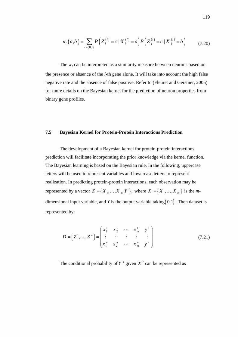
119

( ) ( ) ( )( ) ( ) ( )( ){ }0,1

, | |l l l ll i i j

ca b P Z c X a P Z c X bκ

∈

= = = =∑ j = (7.20)

The can be interpreted as a similarity measure between neurons based on

the presence or absence of the l-th gene alone. It will take into account the high false

negative rate and the absence of false positive. Refer to (Fleuret and Gerstner, 2005)

for more details on the Bayesian kernel for the prediction of neuron properties from

binary gene profiles.

lκ

7.5 Bayesian Kernel for Protein-Protein Interactions Prediction

The development of a Bayesian kernel for protein-protein interactions

prediction will facilitate incorporating the prior knowledge via the kernel function.

The Bayesian learning is based on the Bayesian rule. In the following, uppercase

letters will be used to represent variables and lowercase letters to represent

realization. In predicting protein-protein interactions, each observation may be

represented by a vector { }1, , ,m ,Z X X Y= … where { }1, , mX X X= … is the m-

dimensional input variable, and Y is the output variable taking{ }0,1 . Then dataset is

represented by:

{ }1 1 1 11 2

1

1 2

, ,m

n

n n n nm

x x xD Z Z

y

x x x

⎛ ⎞⎜ ⎟

= = ⎜⎜ ⎟⎝ ⎠

…y

⎟ (7.21)

The conditional probability of given iY iX can be represented as

120

( ) ( )( )

1 11 1

1 1

1, , ,1| , ,

, ,

i i i im ji i i i i

m m i i i ij m

P Y X x X xP Y X x X x

P X x X x

= = == = = =

= =

i

( ) ( )( ){ } ( )1 1

1 10,1

, , | 1 1

, , |

i i i i i im m

i i i i i im my

P X x X x Y P Y

P X x X x Y y P Y y=

= = = ==

= = =∑ = (7.22)

and

( ) ( )10 | , , 1 1| , ,i i i i im mP Y X X P Y X X= = − = 1

i

)

(7.23)

where is the prior probability of taking value and the distribution

for the conditional probability

( i iP Y y= iY iy

( )1 , , |i imP X X Y i

i

can be estimated from the

dataset.

Assuming that the input variables are independent for protein-protein

interactions dataset, Equation (7.22) can be described as follows:

( )1 11| , ,i i i im mP Y X x X x= = =

( ) ( ) ( )( ) ( ) ({ } )1 1

1 10,1

| 1 | 1 1

| |

i i i i i i im m

i i i i i i im my

P X x Y P X x Y P Y

P X x Y y P X x Y y P Y y=

= = = = ==

= = = = =∑ (7.24)

In a similar approach to (Fleuret and Gerstner, 2005) as described in

Equations (7.19) and (7.20), we define a Bayesian kernel for protein-protein

interactions prediction as:

( ) ( )1

, ,m

i j i jl l l

l

k x x x xκ=

=∏ (7.25)

with,

121

( ) ( ) ( ){ }0,1

, | |i j i i i j j jl l l l l l l

yx x P Y y X x P Y y Xκ

∈

= = = =∑ x= (7.26)

The can be interpreted as a similarity measure between protein pairs based

on the l-th position of the feature vector. In this experiment we used the domain

structure as the protein feature for the representation of the feature vector. For the

prior and conditional probability of domains features to facilitate the protein-protein

interactions we used the Appearance Probability matrix that was introduced in (Han

et al., 2004).

lκ

The domain combinations and the appearance frequency information of

domain combinations are obtained from the interacting and non-interacting sets of

protein pairs. The obtained information is stored in the form of a matrix called the

Appearance Probability (AP) matrix. When there are n different proteins

{ }1 2, , , np p p… in a given set of protein pairs and the union of domain combinations

of proteins contains m different domain combinations, { }1 2, , , md d d… , and then the

AP matrix is constructed. The element A in the matrix represents the

appearance probability of domain combination

m m× Pij

,i jd d< > in the given set of protein

pairs. Then the conditional probability in Equation (7.26) can be obtained by:

( )1| APi i il lP Y X x= = = il (7.26)

7.6 Results and Discussion

In this section, the performance of the SVM classifier with the Bayesian

kernel is discussed. The dataset and materials used in this experiment are the same as

described earlier in Section 5.5 but only for domain feature.

122

For constructing the positive interaction set, we represent an interaction pair

by concatenating feature vectors of each proteins pair that are listed in the DIP-

CORE as interacting proteins. Since we use domain feature we include only the

proteins that have structure domains. The resulting positive set for domain feature

contains 1879 protein pairs.

As described in Section 5.6, constructing a negative interaction set using a

random approach to construct the negative data set is an avoidable at this moment.

Furthermore, for the purposes of comparing different kernel methods, the resulting

inaccuracy will be approximately uniform with respect to each kernel method. For

these reasons, the negative interaction set was constructed by generating random

protein pairs. Then, all protein pairs that exist in DIP were eliminated. A negative

interaction set was constructed containing the same number of protein pairs.

In our computational experiment, we employed the LIBSVM (version 2.5)

software and modified it to use the Bayesian kernel defined in Section 7.5. The

performance of the SVM with the Bayesian kernel is compared to the other four

standard kernels described in Section 6.5.

Table 7.1 shows the performance of the SVM with Bayesian kernel using

domain feature with varied threshold. It shows that there is always a trade off

between the sensitivity and specificity. The best cross-validation accuracy is

achieved with threshold of 0.5. The specificity is higher than the sensitivity when

choosing to have best cross-validation accuracy. This means that the Bayesian kernel

can detect the non-interacting protein pairs with a reliable accuracy.

123

Table 7.1: Bayesian Kernel performance with varied threshold using domain feature.

Threshold Sensitivity Specificity Cross-Validation Accuracy

0.1 0.044 0.991 0.5175

0.2 0.243 0.967 0.605

0.3 0.459 0.941 0.7

0.4 0.621 0.899 0.76

0.5 0.774 0.839 0.8065

0.6 0.844 0.727 0.7855

0.7 0.906 0.596 0.751

0.8 0.954 0.461 0.7075

0.9 0.989 0.253 0.621

The performance of the Bayesian kernel compared to the other four standard

kernels is presented in Table 7.2. The Bayesian kernel has significantly improved the

prediction accuracy compared to the linear and polynomial kernel. It also has slightly

improved the prediction accuracy compared to the RBF and sigmoid kernel.

However, it is important to note the Bayesian kernel has the advantage of the

probabilistic output over the RBF and sigmoid kernel. It help biologist to conduct

further analysis on the predicted interacting proteins pairs with high probability.

124

Table 7.2: Bayesian Kernel performance compared to the standard kernels using

domain feature.

Kernel Sensitivity Specificity Cross-Validation accuracy

Linear Kernel 0.726 0.764 0.768

Polynomial Kernel 0.731 0.787 0.772

RBF Kernel 0.742 0.811 0.793

Sigmoid Kernel 0.751 0.805 0.791

Bayesian Kernel 0.774 0.839 0.8065

The ROC curve is also used to compare the performance of the Bayesian

kernel against the standard kernel. Figure 7.2 shows the ROC curve with ROC score

for each kernel. The Bayesian kernel perform better than the standard kernels and has

higher ROC score.

Figure 7.2: The ROC curve for the Bayesian kernel and the standards kernel.

125

The distribution of the probabilistic output for the Bayesian kernel is shown

in Figure 7.3. The Bayesian kernel output a scalar value showing its belief in

classification decision. Each protein pair that was predicted either interacting pair or

non-interacting pair is assigned a likelihood of the predicted value.

Distribution of the Prediction Probabilities

0

100

200

300

400

500

600

700

<10% 10-19%

20-29%

30-39%

40-49%

50-59%

60-69%

70-79%

80-89%

>89%

The Percentage

Num

ber o

f Pro

tein

Pai

rs

Figure 7.3: The distribution of the probabilistic output for the Bayesian kernel

From Figure 7.3, we can see that the number of protein pairs that have been

predicted as interacting pairs with likelihood bigger than 89% is less than 100 pairs

which is very small number compared to number interacting protein in the training

dataset (1879). However, biologist can carry out experiments to validate the results

for the protein pairs that were predicted as interacting pairs with high likelihood. It is

time-consuming and costly to carry out experiments to validate the results of all

predicted protein pairs.

Comparing protein-protein interaction prediction systems with the other

existing systems is always a difficult task. The reason is that, most of the authors

used different type of data, experimental setup, and evaluation measures.

126

Several research studies in the literature reported higher accuracy than it is

achieved in this research. The main reason behind these different performances is the

construction of the negative dataset for protein-protein interactions. There is no

experimentally confirmed non-interacting protein pairs made available by biologist.

This contributes to the unavailability of benchmark data that facilitate the

comparison of different algorithms. For instance, Chung et al. (2004) reported

accuracy of 94% by using hydrophobicity as the protein feature. The reason for this

high accuracy lies in the approach of constructing the negative interaction dataset.

They assign random value to each amino acid in the protein pair sequence. This leads

to get new pairs that considered negative interacting pairs and greatly different from

the positive interacting pairs in the training dataset. This effect leads to simplify the

learning task and artificially raise classification accuracy for training data. There is

no guarantee, however, that the generalized classification accuracy will not degrade

if the predictor is presented with new, previously unseen data which are hard to

classify.

In Table 7.3 we compare the performance of the Bayesian kernel developed

in this study with some of cited literature that use same datasets and use similar

approach in constructing the negative interactions.

Table 7.3: Performance comparison with the cited literature.

Reference Method Accuracy ROC score

Bock & Gough, (2001) SVM 0.8096 —

Gomez et al., (2003) attraction-repulsion model — 0.818

Dohkan et al., (2004) SVM 0.788 —

Huang et al., (2004) SVM 0.7957 —

Our Approach Bayesian Kernel 0.8065 0.8670

127

As shown in Table 7.3, the Bayesian kernel outperforms most of the related

cited literature in terms of ROC score. However, it should be noted that some of the

cited literature did not report an ROC score for their method performance. Also in

term of prediction accuracy the Bayesian kernel achieve a comparable and slightly

better accuracy than most of the cited work.

7.7 Summary

This chapter reports the development and application performance of the

Bayesian kernel for the prediction of protein-protein interactions. The Bayesian

kernel was developed based on the Bayes’ Rule. The performance results of the

Bayesian kernel outperformed most of the cited related work with ROC score of

0.8670. However, the comparison with some other works is not feasible due to the

fact that different datasets were used. In addition, constructing negative set of non-

interacting proteins is still the source of the varied reported accuracy. This is

because, until now there is no experimentally confirmed non-interacting proteins

dataset. Different cited work use different random method to generate non-

interacting protein pairs. In conclusion, the Bayesian kernel provide a better

performance as well as probabilistic output that could help biologist to carry out

further analysis.

CHAPTER 8

CONCLUSION AND FUTURE WORK

This chapter draws general conclusion of the review of literature,

methodology, experimental work, analysis, and the discussion of this research work.

The output and results of the developed methods for protein-protein interactions

prediction are concluded and summarized in this chapter. This chapter also presents

the findings and the contributions of this research. In addition, potential future work

is suggested and presented in this chapter.

8.1 Conclusion

It has been established that the rapid development of molecular biology and

achievements of modern technology have raised many questions of great

bioinformatics interest and there is a growing need to develop, apply and analyze

effective and efficient learning methods to improve managing and annotating the

novel biological sequences.

Predicting protein-protein interactions is one of the key topics in the post-

genomic era. The interactions between proteins are important for many biological

functions. Almost all processes in of molecular biology are affected by protein-

protein interactions. Therefore, useful methodologies and algorithms for prediction

of protein-protein interactions have to be developed and implement. In this thesis

several problems of protein-protein interactions prediction have been investigated.

129

The first objective of this research is to study and investigate different protein

sequence feature for the prediction of protein-protein interactions using the support

vector machines. In chapter 5 we compare the use of the domain structure and

hydrophobicity properties as protein sequence features. This is motivated by several

related work in the literature as discussed in chapter 5. In this experiment we

consider four features, namely: domain, domain with score, hydrophobicity, and

hydrophobicity with scale. The results show that domain feature achieves cross-

validation accuracy of 79.4372% and ROC score of 0.8480. This is slightly better

accuracy than when using hydrophobicity scale feature. However, domain feature

prediction performance is much better in terms ROC score and running time. For

domain feature only around 34 seconds is need for the cross-validation experiment

while hydrophobicity scale feature takes around 9.6 hours. Other results show that

domain score is not important and it is informative enough to consider only the

existence of domains structure in the protein pairs. However, hydrophobicity scale

feature achieve slightly better accuracy than the hydrophobicity feature but with

more running time. It is important here to note that the performance of the prediction

system is far better than an absolute random approach which has ROC score of 0.5.

This indicates that the difference between interacting and non-interacting protein

pairs can be learned from the available data.

The prediction approach reported in Chapter 5 generates a binary decision

regarding potential protein-protein interactions based on training set consists of

positive dataset (interacting proteins) and negative dataset (non-interacting proteins).

Based on the fact that information about protein-protein interactions has been

accumulated by various experimental techniques, constructing a dataset of

interacting protein is feasible and straight forward. However, there are no

experimentally confirmed non-interacting protein pairs. Hence, constructing non-

interacting pairs for training the learning system is a challenge. In Chapter 5

experiment, we use a randomizing method to generate negative dataset. This is

acceptable for comparing features or algorithms since the error will be uniform on

the different features or algorithms.

130

Given the fact that only information about interacting proteins (positive

dataset) are available and sampled well, the problem of predicting protein-protein

interaction is essentially one-class classification problem. In Chapter 6, using only

positive examples (interacting protein pairs) in training phase, the one-class SVM

was implemented and applied. It achieves accuracy of about 80% using the domain

features with the RBF kernel. These results indicate that the difference between

interacting and non-interacting protein pairs can be learned from the available

positive data using one-class classifier. It is also important to note that the choice of

the parameters has a clear impact on the classifier performance.

Appropriate parameters for the one-class SVM with the standard four kernels

are set by the cross-validation process. The results show that the one-class SVM is

very sensitive to the choice of parameters. Even though, the best results were found

by the RBF kernel, it could give as low accuracy as 29% with unsuitable choice of

parameters.

The results of applying the one-class SVM imply that protein-protein

interaction can be predicted using one-class classifier with comparable accuracy to

the binary classifiers that use artificially constructed negative dataset. When using

randomly generated negative dataset, there is no guarantee that the generalized

classification accuracy will not degrade if the predictor is presented with new,

previously unseen data which are hard to classify. In our work we used only positive

data in the training set. In this case we don’t need any artificially generated negative

data for the training phase. We believe this approach makes the learning problem

more realistic and ensure that our training accuracy better reflects generalized

classification accuracy.

SVM gives its classification output as a binary decision. However, it is

desirable to have a probabilistic approach that output a scalar value showing its belief

in the classification decision. The Bayesian kernel for SVM gives its output as

probabilities. Besides, the Bayesian kernel can improve the classifier performance by

incorporated the probability characteristic of the available experimental protein-

protein interactions data. Each protein pair that was predicted either interacting pair

or non-interacting pair is assigned a likelihood of the predicted value.

131

The development and implementation of the Bayesian kernel for the SVM

was presented in Chapter 7. The Bayesian kernel performs better than the standard

kernels and has higher ROC score of 0.8670. The Bayesian kernel outperforms most

of the related cited literature in terms of ROC score. However, it should be noted that

some of the cited literature did not report an ROC score for their method

performance. Also in term of prediction accuracy the Bayesian kernel achieve a

comparable and better accuracy compared to most of the cited work.

The overall results indicate that it is informative enough to consider the

existence of domains structure in the protein pairs to facilitate the prediction of

protein-protein interactions. The Bayesian kernel results with probabilistic output

could help biologist to conduct further analysis on the predicted interacting proteins

pairs with high likelihood score.

In conclusion the result of this research suggests that protein-protein

interactions can be predicted from domain structure and hydrophobicity properties as

protein sequence features. Consequently, these results show the possibility of

proceeding directly from the automated identification of a cell’s gene products to

inference of the protein interaction pairs, facilitating protein function and cellular

signaling pathway identification.

8.2 Research Contributions

This research focuses on predicting protein-protein interactions with reliable

accuracy. The contributions of this research are summarized as follows:

• Investigating and comparing the two main protein sequence features for

the prediction of protein-protein interactions using the support vector

machines.

132

• Modeling and solving the problem protein-protein interactions a one-class

classification problem using the one-class support vector machines.

• Developing and implementing the Bayesian kernel for SVM to

incorporate the probabilistic information about the protein-protein

interaction and provide a probabilistic output in the classification

decision.

8.3 Future Work

Hopefully, the output of the research can be a motivation for further

investigation in the field of protein-protein interactions predictions. In this thesis,

protein-protein interactions prediction task successfully performed. In this research

some new directions and some important and useful contributions to the efforts to

predict protein-protein interactions have been presented. In this section we will

outline some of the possible future work directions.

Based on the important issue of feature selection in machine learning,

automated methods have to be developed. Suitable features would not only be

computationally efficient for the techniques presented in this thesis but will also be a

useful contribution in general classification problems. For the sequence features

presented and compared in Chapter 5, further investigation of the other possible

sequence features is significantly important.

The issue of constructing negative dataset (non-interacting proteins) is a

difficult task. This is due to the fact that there are no experimentally confirmed non-

interacting proteins have been made available. Hence, investigating different

approach to construct the negative set for binary classifiers represent a big challenge.

Several methods have been recently investigated in the literature. However, a reliable

assessment of the classifiers performance using different approaches for negative

dataset construction is needed.

133

It is also important to note that the available protein-protein interactions data

are collected using different experimental techniques. The overlaps between these

data are very small. Therefore there is a need for a development of computation

techniques that validate the experimental results and assess the reliability of the

experimental techniques.

Similar methods of prediction and classification in fields rather than

Bioinformatics can successfully utilize variety of techniques and tools used in this

research such as the one-class SVM and the Bayesian kernel approach.

Since the research in Bioinformatics field in general and the protein

secondary structure prediction domain in particular is increasing rapidly, the need for

a “utility and statistical package for Bioinformatics” that successfully arranges data

for input and helps in the analysis and assessment of the output becomes crucial. This

will save considerable time for the research in Bioinformatics.

8.4 Closing

This chapter concludes and summarizes the research work discussed in this

thesis. The chapter also presents and highlights the contributions and findings of this

research. Recommendations for further work and future research directions in the

domain of this work are also coined and proposed in this chapter. Hopefully this

research gives an idea and spreading knowledge in the research field, especially in

bioinformatics.

134

RELATED PUBLICATIONS

Hany Alashwal, Safaai Deris and M. Razib Othman. (2006). One-Class Support

Vector Machines for Protein-Protein Interactions Prediction. The International

Journal of Biomedical Sciences, 1(2):120-127.

Nazar Zaki, Safaai Deris and Hany Alashwal. (2006). Protein-Protein Interaction

Detection Based on Substring Sensitivity Measure. The International Journal of

Biomedical Sciences, 1(2):148-154.

Hany Alashwal, Safaai Deris and M. Razib Othman. (2006). Comparison of Domain

and Hydrophobicity Features for the Prediction of Protein-Protein Interactions

using Support Vector Machines. The International Journal of Information

Technology, 3(1):18-24.

Hany Alashwal, Safaai Deris, M. Razib Othman and Mohd Saberi Mohamad. (2006).

One-Class Classifier to Predict Protein-Protein Interactions based on

Hydrophobicity Properties. In the International Symposium on Biomedical

Engineering (ISBME’06), November 8-10. Bangkok, Thailand.

Hany Alashwal, Safaai Deris and M. Razib Othman. (2006). Predicting Proteins

Interactions from Protein Sequence Features using Support Vector Machines. In

the International Conference on Bioinformatics & Computational Biology

(BioComp’06), June 26-29. Las Vegas, Nevada, USA.

Hany Alashwal, Safaai Deris and M. Razib Othman. (2006). Support Vector

Machines for Predicting Protein-Protein Interactions using Domains and

Hydrophobicity Features. In the International Conference on Computing and

Informatics (ICOCI 2006), June 6-8. Kuala Lumpur, Malaysia.

Hany Alashwal, Safaai Deris and M. Razib Othman. (2006). Predicting Protein-

Protein Interactions as a One-Class Classification Problem. In FSKSM

Postgraduate Annual Research Seminar, May 24-25. Skudai, Johor, Malaysia.

135

Safaai Deris, Hany Alashwal, Mohd Saberi , Yeo Lee Chin, Muhammad Razib

Othman, Yuslina Zakaria, Suhaila Zainudin, Nazar Zaki, Saad Othman, and

Satya Arjunan. (2005). Bioinformatics: A Tool for Bio-Knowledge Generation.

In the International Conference on Information Technology and Multimedia

(ICIMU 2005), November 22-24. Kuala Lumpur, Malaysia.

Hany Alashwal and Safaai Deris. (2005). Computational Prediction of Protein-

Protein Interactions Based on Protein Domain Structure and Hydrophobic

Properties. In the International Symposium on Bio-Inspired Computing (BIC05).

September 5-7. Johor, Malaysia

Hany Alashwal, Safaai Deris, M. Razib Othman, Azmee Awang and Zalmiyah

Zakaria. (2004). Predicting Protein-Protein Interactions from Primary Structure

using Support Vector Machines. In the International Conference on

Bioinofromatics (InCoB2004), September 5-8. Aotea Centre, Auckland, New

Zealand.

136

REFERENCES

Abascal, F. and Valencia, A. (2003). Automatic annotation of protein function based

on family identification. Proteins. 50:683-692.

Alberts, B., Johnson, A., Lewis, J., Raff, M., Roberts, K., and Walter, P. (2002).

Molecular Biology of the Cell (4th edition). Garland Science.

Altschul, S.F., Madden, T.L., Schaffer, A.A., Zhang, J., Zhang, Z., Miller, W. and

Lipman, D.J. (1997). Gapped BLAST and PSI-BLAST: a new generation of

protein database search programs. Nucleic Acids Research. 25: 3389-3402.

Attwood, T. K. and Miller, C. J. (2001). Which craft is best in bioinformatics?

Computers and Chemistry. 25:327{337.

Bairoch, A. (2000). The ENZYME database in 2000. Nucleic Acids Res 28:304-305.

Bartel, P.L. and Fields, S. (eds) (1997). The yeast two-hybrid system. In Advances in

Molecular Biology. Oxford University Press, New York.

Bateman A., Coin, L., Durbin, R., Finn, R.D., Hollich, V., Griffiths-Jones, Khanna,

S., Marshall, A., Moxon, S.E., Sonnhammer, L.L., Studholme, D.J., Yeats, C.

and Eddy S.R. (2004). The Pfam: Protein Families Database. Nucleic Acids

Research Database Issue. 32:D138-D141

Ben-Hur, A. and Noble, W.S. (2005). Kernel methods for predicting protein-protein

interactions. Bioinformatics. 21:i38–i46.

Bishop, C. (1994). Novelty detection and neural network validation. IEE Proceedings

on Vision, Image and Signal Processing. Special Issue on Applications of Neural

Networks. 141(4):217–222.

Bock, J.R. and Gough, D.A. (2001). Predicting protein-protein interactions from

primary structure. Bioinformatics. 17(5):455-60.

Bork, P., Jensen, L.J., von Mering, C., Ramani, A.K., Lee, I. and Marcotte, E.M.

(2004). Protein interaction networks from yeast to human. Current Opinion

Structural Biology. 14:292–299.

137

Boser, B.E., Guyon, I.M., and Vapnik, V.N. (1992). A training algorithm for optimal

margin classifiers. In Haussler, D.(editor) Proceedings of the 5th Annual ACM

Workshop on Computational Learning Theory. Pittsburgh, PA, ACM:144-152.

Boulton, S.J., Gartner, A., Reboul, J., Vaglio, P., Dyson, N., Hill, D.E. and Vidal, M.

(2002). Combined functional genomic maps of the C elegans DNA damage

response. Science. 295:127-131.

Brown, M. P., Grundy, W. N., Lin, D., Cristianini, N., Sugnet, C. W., Furey, T. S.,

Ares, M. JR.and Haussler, D. (2000). Knowledge-based analysis of microarray

gene expression data by using support vector machines. Proceedings of National

Academy of Sciences USE. 97:262-267.

Chang, C.C. and Lin, C.J. (2001). LIBSVM: a library for support vector machines.

Software available at http://www.csie.ntu.edu.tw/~cjlin/libsvm. (24/3/2005).

Chung, Y., Kim, G., Hwang, Y. and Park, H. (2004). Predicting Protein-Protein

Interactions from One Feature Using SVM. In IEA/AIE’04 Conf. Proc. May 17-

20. Ottawa, Canada.

Clare, A. and King, R.D. (2002). Machine learning of functional class from phenotype

data. Bioinformatics. 18: 160-166.

Cortes, C. and Vapnik, V. (1995). Support vector networks. Machine Learning.

20:273-297.

Costanzo, M.C., Crawford, M.E., Hirschman, J.E., Kranz, J.E., Olsen, P., Robertson,

L.S., Skrzypek, M.S., Braun, B.R., Hopkins, K.L., Kondu, P., Lengieza, C., Lew-

Smith, J.E., Tillberg, M. and Garrels, J.I. (2001). YPD™, PombePD™, and

WormPD™: model organism volumes of the BioKnowledge library, an integrated

resource for protein information. Nucleic Acids Research. 29: 75 79.

Craig, R.A. and Liao, L. (2007). Phylogenetic tree information aids supervised

learning for predicting protein-protein interaction based on distance matrices.

BMC Bioinformatics. 8:6.

Cramer, P., Bushnell, D.A., and Kornberg, R.D. (2001). Structural basis of

transcription: RNA polymerase II at 2.8 angstrom resolution. Science. 292:1863–

1876.

Deane, C.M., Salwinski, L., Xenarios, I. and Eisenberg, D. (2001). Protein

interactions: Two methods for assessment of the reliability of high throughput

observations. Molecular & Cellular Proteomics. 15: 349-356.

138

Deng, M., Zhang, K., Mehta, S., Chen, T. and Sun, F.Z. (2002). Prediction of protein

function using protein-protein interaction data. The first IEEE bioinformatics

conference, Stanford University. CSB2002:197-206.

Dohkan, S., Koike, A. and Takagi, T. (2003). Support Vector Machines for Predicting

Protein-Protein Interactions. Genome Informatics. 14:502–503

Dohkan, S., Koike, A. and Takagi, T. (2004). Prediction of protein-protein

interactions using Support Vector Machines. In Proceedings of the Fourth IEEE

Symposium on BioInformatics and BioEngineering (BIBE2004). Taitung, Taiwan.

576-584.

Dohkan, S., Koike, A. and Takagi, T. (2006). Improving the Performance of an SVM-

Based Method for Predicting Protein-Protein Interactions. In Silico Biology.

6(6):515 – 529.

Donaldson, I., Martin, J., de Bruijn, B., Wolting, C., Lay, V., Tuekam, B., Zhang, S.,

Baskin, B., Bader, G.D., Michalickova, K., Pawson, T., and Hogue, C.W. (2003).

PreBIND and Textomy--mining the biomedical literature for protein-protein

interactions using a support vector machine. BMC Bioinformatics. 4:11.

Eisen, M., Spellman, P., Brown, P. and Botstein, D. (1998). Cluster analysis and

display of genome-wide expression patterns. PNAS. 95:14863-14868.

Eisenberg, D., Marcotte, E. M., Xenarios, I. and Yeates, T.O. (2000). Protein function

in the post-genomic era. Nature. 405: 823-826.

Eisenberg, D., Schwarz, E., Komaromy, M. and Wall, R. (1984). Analysis of

membrane and surface protein sequences with the hydrophobic moment plot. J.

Mol. Biol. 179:125-142.

Enright, A.J., Iliopoulos, I., Kyrpides, N.C., and Ouzounis, C.A. (1999). Protein

interaction maps for complete genomes based on gene fusion events. Nature.

402:86–90.

Fleuret, F. and Gerstner, W. (2005). A Bayesian Kernel for the Prediction of Neuron

Properties from Binary Gene Profiles. Proceedings of the IEEE International

Conference on Machine Learning and Applications. Special session Applications

of Machine Learning in Medicine and Biology (ICMLA):129–134.

Friess, T., Cristianini, N. and Campbell, C. (1998). The kernel-adatron a fast and

simple training procedure for support vector machines. In Shavlik, J.(editor)

Proceedings of the 15th International Conference on Machine Learning. July 24-

27. Madison, Wisconsin USA.

139

Gallet, X., Charloteaux, B., Thomas, A. and Brasseur, R. (2000). A fast method to

predict protein interaction sites from sequences. J. Mol. Biol. 302:917-926.

Gavin, A.C., Bosche, M., Krause, R., Grandi, P., Marzioch, M., Bauer, A., Schultz, J.,

Rick, J.M., Michon, A.M., Cruciat, C.M. et al . (2002). Functional organization of

the yeast proteome by systematic analysis of protein complexes. Nature. 415:141-

147

Gharakhanian, E., Takahashi, J., Clever, J., and Kasamatsu, H. (1998). In vitro Assay

for Protein-Protein Interaction: Carboxyl-Terminal 40 Residues of Simian Virus

40 Structural Protein VP3 Contain a Determinant for Interaction with VP1. PNAS

85(18):6607-6611.

Goffard, N., Garcia,V., Iragne, F., Groppi, A. and De Daruvar,A. (2003). IPPRED:

Server for proteins interactions inference. Bioinformatics. 19:903–904

Gomez, S. M., Noble, W.S. and Rzhetsky, A. (2003). Learning to predict protein-

protein interactions from protein sequences. Bioinformatics.19(15):1875-1881.

Han, D.S., Kim,H.S., Jang, W.H. and Lee, S.D. (2004). PreSPI: A Domain

Combination Based Prediction System for Protein-Protein Interaction. Nucleic

Acids Research. 32(21): 6312-6320.

Harrington, H.C., Rosenow, C. and Retief, J. (2000). Monitoring gene expression

using DNA microarrays. Curr. Opin. Microbiol. 3:285-291.

Heckerman, D., Geiger, D., and Chickering, D. (1995). Learning Bayesian networks:

The combination of knowledge and statistical data. Machine Learning. 20:197-

243.

Henikoff, S. and Henikoff J.G., (1994). Protein family classification based on

searching a database of blocks. Genomics. 19:97-107.

Hermjakob, H., Montecchi-Palazzi, L., Bader, G., Wojcik, J., Salwinski, L., Ceol, A.,

Moore, S., Orchard, S., Sarkans, U., von Mering, C., et al. (2004). The HUPO

PSI's Molecular Interaction format - A community standard for the representation

of protein interaction data. Nature Biotechnology. 22:177-183.

Hishigaki, H., Nakai, K., Ono, T., Tanigami, A. and Takagi, T. (2001). Assessment of

prediction accuracy of protein function from protein-protein interaction data.

Yeast. 18:523-531.

Ho, Y., Gruhler, A., Heilbut, A., Bader, G.D., Moore, L., Adams, S., Millar, A.,

Taylor, P., Bennett, K., Boutilier, K. et al. (2002). Systematic identification of

140

protein complexes in Saccharomyces cerevisiae by mass spectrometry. Nature.

415:180 183.

Hodgman, T. C. (2000). A historical perspective on gene/protein functional

assignment. Bioinformatics. 16:10-15

Hong, E.L., Balakrishnan, R., Christie, K.R., Costanzo, M.C., Dwight, S.S., Engel,

S.R., Fisk, D.G., Hirschman, J.E., Livstone, M.S., Nash, R., Oughtred, R., Park,

J., et al., (2005). Saccharomyces Genome Database.

http://www.yeastgenome.org/ (16/2/2005).

Hopp, T.P. and Woods, K.R. (1981). Predicting of protein antigenic determinants

from amino acid sequences. Proc. Natl Acad. Sci. USA. 7 8(6): 3824-3828 .

Hsu, C.W. and Lin, C. J. (2002). A simple decomposition method for support vector

machines. Machine Learning. 46:291-314.

Huang, C., Morcos, F., Kanaan, S.P., Wuchty, S., Chen, D.Z., and Izaguirre, J.A.

(2007). Predicting Protein-Protein Interactions from Protein Domains Using a Set

Cover Approach. EEE/ACM Transactions on Computational Biology and

Bioinformatics (TCBB). 4(1):78-87.

Huang, Y., Frishman, D., Muchnik, I. (2004). Predicting Protein-Protein Interactions

by a Supervised Learning Classifier. Computational Biology and Chemistry , 28,

4, 291-301.

Ito, T., Tashiro, K., Muta, S., Ozawa, R., Chiba, T., Nishizawa, M., Yamamoto, K.,

Kuhara, S. and Sakaki, Y. (2000). Toward a protein-protein interaction map of the

budding yeast: a comprehensive system to examine two-hybrid interactions in all

possible combinations between the yeast proteins. Proc. Natl. Acad. Sci. USA.

97: 1143-1147.

Jansen, R., Yu, H., Greenbaum, D., Kluger,Y., Krogan, N.J., Chung, S., Emili, A.,

Snyder, M., Greenblatt, J.F. and Gerstein, M. (2003). A Bayesian networks

approach for predicting protein-protein interactions from genomic data. Science.

302: 449-53.

Japkowicz, N. (1999). Concept-Learning in the absence of counterexamples: an

autoassociation-based approach to classification. PhD thesis, New Brunswick

Rutgers, The State University of New Jersey.

Jensen, F. (1996). An Introduction to Bayesian Networks. UCL Press, London.

Jones, S. and Thornton J. M. (1997). Prediction of protein-protein interaction sites

using patch analysis. J. Mol. Biol. 272:133-143.

141

Karplus, K., Kimmen, S., Barrett, C., Cline, M., Haussler, D., Hughey, R., Holm, L.

and Sander, C. (1997). Predicting protein structure using hidden Markov models.

Proteins: Structure, Function, and Genetics, Suppl. 1:134-139.

Keerthi, S.S. and C.J. Lin (2003). Asymptotic behaviors of support vector machines

with Gaussian kernel. Neural Computation. 15(7):1667–1689.

Kim, W.K., Park, J., and Suh, J.K. (2002). Large scale statistical prediction of protein-

protein interaction by potentially interacting domain (PID) pair. Genome

Informatics. 13:42-50.

King, R.D., Karwath, A., Clare, A. and Dehaspe, L. (2001). The utility of different

representations of protein sequence for predicting functional class.

Bioinformatics. 17: 445-454.

Kini, R.M. and Evans, H.J. (1996). Prediction of potential protein-protein interaction

sites from amino acid sequence identification of a fibrin polymerization site.

FEBS letters. 385: 81-86.

Koike, A. and Takagi, T. (2003). Prediction of Protein Interaction Sites and Protein-

Protein Interaction Pairs Using Support Vector Machines. Genome Informatics.

14:500-501.

Koller, D. (1999). Probabilistic Relational Models Source. Lecture Notes In Computer

Science. 1634: 3 - 13

Korf, I., Yandell, M., and Bedell, J. (2003). BLAST: Basic Local Alignment Search

Tool. O’Reilly & Associates.

Kuhn, H. W. and Tucker, A. W. (1951). Nonlinear programming. In Proceedings of

2nd Berkeley Symposium on Mathematical Statistics and Probabilistic. Berkeley,

University of California:481-492.

Larrañaga,P., Gallego, M.Y. Sierra, B. Urkola,L., and Michelena, M.J. (1997).

Bayesian networks, rule induction and logistic regression in the prediction of the

survival of women suffering from breast cancer. Lecture Notes in Artificial

Intelligence. 1323. E. Costa, A. Cardoso (eds.):303-308. Springer-Verlag.

Legrain, P., Wojcik, J., and Gauthier, J. (2001) Protein-protein interaction maps: a

lead towards cellular functions. Trends in Genet. 17:346-352.

Letovsky, S., and Kasif, S. (2003). Predicting protein function from protein-protein

interaction data: a probabilistic approach. Bioinformatics Vol. 19 Suppl. 1:i197–

i204.

142

Lichtarge, O., Bourne, H.R. and Cohen, F.E. (1996). An evolutionary trace method

defines binding surfaces common to protein families. J. Mol. Biol. 257:342-358.

Lin, N., Wu, B., Jansen, R., Gerstein, M., and Zhao H. (2004). Information

assessment on predicting protein-protein interactions. BMC Bioinformatics.

5:154.

Lodish, H., Berk, A., Matsudaira, P., Kaiser, C.A., Krieger, M., Scott, M.P., Zipurksy,

S.L., and Darnell, J. (2004). Molecular Cell Biology 5th ed. WH Freeman and

Company: New York, NY.

Lu, L., Lu, H., and Skolnick, J. (2002). MULTIPROSPECTOR: An algorithm for the

prediction of protein-protein interactions by multimeric threading. Proteins. 49:

350-364.

Marcotte, E.M., Pellegrini, M., Ng, H., Rice, D.W., Yeates, T.O., and Eisenberg, D.

(1999). Detecting Protein Function and Protein-Protein Interactions from Genome

Sequences. Science. 285(5428):751–753.

Marcotte, E.M., Xenarios, I., van Der Bliek, A.M. and Eisenberg, D. (2000).

Localizing proteins in the cell from their phylogenetic profiles, Proc. Natl. Acad.

Sci. USA 97:12,115–12,120

Moya, M., Koch, M., and Hostetler, L. (1993). One-class classifier networks for target

recognition applications. In Proceedings world congress on neural networks.

Portland, OR. International Neural Network Society, INNS:797–801.

Mulder, N.J., Apweiler, R., Attwood, T. K., Bairoch, A., Barrell, D., Bateman, A.,

Binns, D., et al., (2003). The InterPro Database brings increased coverage and

new features. Nucleic Acids Research. 31:315-318.

Müller, K. R., Mika, S., Ratsch, G., Tsuda, K., & Schölkopf, B. (2001). An

introduction to kernel-based learning algorithms. IEEE Transactions on Neural

Networks. 12(2):181–201.

Newman, J. R., Wolf, E., and Kim, P. S. (2000). A computationally directed screen

identifying interacting coiled coils from Saccharomyces cerevisiae. Proc. Natl.

Acad. Sci. U.S.A. 97:13203–13208

Ng, S., Zhang, Z. and Tan, S. (2003). Integrative approach for computationally

inferring protein domaininteractions. Bioinformatics. 19:923-929.

Niculescu, R., and Mitchell, T. (2006). Bayesian network learning with parameter

constraints. Journal of Machine Learning Research. 7:1357–1383.

143

Norin, M. and Sundstrom, M. (2002). Structural proteomics: developments in

structure-to-function predictions. Trends in Biotechnology. 20:79-84.

Ofran, Y. and Rost, B. (2003). Predict protein–protein interaction sites from local

sequence information. FEBS Letters. 544:236–239.

Osuna, E., Freund, R., and Girosi, F. (1997). An improved training algorithm for

support vector machines. In Proc of IEEE NNSP’97. Amelia Island:24-26.

Oyama, T., Kitano, K., Satou, K. and Ito, T. (2000). Mining association rules related

to protein-protein interactions. Genome Informatics. 11:358–359.

Palsson, B. (2000). The challenges of in silico biology. Nature Biotechnology.

18:1147-1150.

Pawson, T. and Nash, P. (2003). Assembly of cell regulatory systems through protein

interaction domains. Science. 300:445–452.

Pazos, F., Helmer-Citterich, M., Ausiello, G. and Valencia, A. (1997). Correlated

mutations contain information about protein-protein interaction. J. Mol. Biol.

271:511-523.

Pearson,W.R. (2000). Flexible sequence similarity searching with the FASTA3

program package. Methods Mol. Biol. 132:185-219.

Pellegrini, M., Marcotte, E., Thompsom, M.J., Eisemberg, D. and Yeates, T.O.

(1999). Assigning protein functions by comparative genome analysis: Protein

phylogenetic profiles. Proc. Nat. Acad. Sci. 96:4285-4288.

Phizicky, E.M. and Fields, S. (1995). Protein-Protein Interactions: Methods for

Detection and Analysis. Microbiological Reviews (Mar.):94-123.

Punta, M. and Rost, B. (2005). PROFcon: novel prediction of long-range contacts.

Bioinformatics. 21:2960–2968.

Rigaut, G., Shevchenko, A., Rutz, B., Wilm, M., Mann, M., and Seraphin, B. (1999).

A generic protein purification method for protein complex characterization and

proteome exploration. Nature Biotechnology. 17(10):1030-1032.

Riley, R., Lee, C., Sabatti, C., and Eisenberg , D. (2005). Inferring protein domain

interactions from databases of interacting proteins. Genome Biology. 6:R89

Ritter, G. and Gallegos, M. (1997). Outliers in statistical pattern recognition and an

application to automatic chromosome classification. Pattern Recognition Letters,

18:525–539.

144

Salamov, A.A. and Solovyev, V.V. (1995). Prediction of protein secondary structure

by combining nearest- neighbor algorithms and multiple sequence alignments. J.

Mol. Biol. 247:11-15.

Salwinski, L. and Eisenberg, D. (2003) Computational methods of analysis of

protein–protein interactions. Curr. Opin. Struct. Biol. 13:377–382.

Schölkopf, B. Smola, A., and Muller K.R. (1999). Kernel principal component

analysis. MIT Press.

Schölkopf, B., and Smola, A. (2002). Learning with kernels—support vector

machines, regularization, optimization and beyond. Cambridge, MA: MIT Press.

Schwikowski, B., Uetz, P. and Fields, S. (2000). A network of protein-protein

interactions in yeast. Nature Biotechnology 18:1257-1261.

Selbach, M. and Mann, M. (2006). Protein interaction screening by quantitative

immunoprecipitation combined with knockdown (QUICK). Nature Methods.

3:981-983.

Shawe-Taylor, J. and Cristianini, N. (2000). An Introduction to Support Vector

Machines and Other Kernel-based Learning Methods. Cambridge University

Press.

Shawe-Taylor, J. and Cristianini, N. (2004). Kernel Methods for Pattern Analysis.

Cambridge University Press.

Shen, J., Zhang, J., Luo, X., Zhu, W., Yu, K., Chen, K., Li, Y., and Jiang, H. (2007).

Predicting protein–protein interactions based only on sequences information.

PNAS. 104:4337-4341.

Shin, H.J., Eom D.H. and Kim S.S. (2005). One-class support vector machines: an

application in machine fault detection and classification. Computers and

Industrial Engineering. 48(2):395–408.

Sikora, M., Morcos, F., Costello, D.J., and Izaguirre J.A. (2007). Bayesian Inference

of Protein and Domain Interactions Using the Sum-Product Algorithm. Proc.

Information Theory and Applications Workshop, San Diego, Jan. 29.

Sonnhammer, E.L.L. and Kahn, D. (1994). Modular arrangement of proteins as

inferred from analysis of homology. Protein Science. 3:482-492.

Tipping, M. (1999). The relevance vector machine. In Advances in Neural

Information Processing Systems. 12.

Tong, A.H, Drees, B., Nardelli, G., Bader G.D., Brannetti, B., Castagnoli, L.,

Evangelista, M., Ferracuti, S., Nelson, B., Paoluzi, S., et al. (2002). A combined

145

experimental and computational strategy to define protein interaction networks

for peptide recognition modules. Science. 295:321-324.

Tong, A.H., Evangelista, M., Parsons, A.B., Xu, H., Bader, G.D., Page, N., et al.

(2001). Systematic genetic analysis with ordered arrays of yeast deletion mutants.

Science. 294:2364–2368.

Uetz, P. and Vollert, C.S. (2005). Protein-Protein Interactions. Encyclopedic

Reference of Genomics and Proteomics in Molecular Medicine (ERGPMM),

Springer Verlag. 16:1548-1552.

Uetz, P., Giot, L., Cagney, G., Mansfield, T.A., Judson, R.S., Knight, J.R., Lockshon,

D., Narayan, V., Srinivasan, M., Pochart, et al. (2000). A Comprehensive analysis

of protein-protein interactions in Saccharomyces cerevisiae. Nature 403:623 627.

Vapnik V.N. (1995). The Nature of Statistical Learning Theory. Springer.

Vazquez A., Flammini, A., Maritan, A., and Vespignani, A. (2003). Global protein

function prediction in protein-protein interaction networks. Nature Biothech.

21:697-702.

Vert, J.P., Tsuda, K., and Schölkopf, B. (2004). A Primer on Kernel Methods

In: Kernel Methods in Computational Biology. MIT Press.

Voet, D. and Voet, J.G. (2004). Biochemistry. Vol 1 3rd ed. Wiley: Hoboken, NJ.

von Mering, C., Krause, R., Snel, B., Cornell, M., Oliver, S.G., Fields, S., and Bork,

P. (2002). Comparative assessment of large-scale data sets of protein–protein

interactions. Nature. 417(6887):399–403.

Walhout, A. and Vidal, M. (2001). Protein interaction maps for model organisms.

Nature Reviews Molecular Cell Biology. 2:55-62.

Walhout, A.J., Reboul, J., Shtanko, O., Bertin, N., Vaglio, P., Ge, H., Lee, H.,

Doucette-Stamm, L., Gunsalus, K.C., Schetter, A.J., Morton, D.G., Kemphues,

K.J., Reinke, V., Kim, S.K., Piano, F., Vidal, M., (2002). Integrating interactome,

phenome, and transcriptome mapping data for the C. elegans germline. Current

Biology. 12:1952–1958.

Wojcik, J. and Schachter, V. (2001) Protein-protein interaction map inference using

interacting domain profile pairs. Bioinformatics. 17:296–305.

Wu, X., Zhu, L., Guo, J., Zhang D., and Lin K. (2006). Prediction of yeast protein–

protein interaction network: insights from the Gene Ontology and annotations.

Nucleic Acids Research. 34(7):2137-2150.

146

Xenarios, I., Salwinski, L., Duan, X.J., Higney, P., Kim, S.M., and Eisenberg, D.,

(2002). DIP: the Database of Interacting Proteins: a research tool for studying

cellular networks of protein interactions. Nucl. Acids. Res. 30(1):303- 305.

Young, L., Jernigan, R.L., and Covell, D.G. (1994). A role for surface hydrophobicity

in protein-protein recognition. Protein Science. 3:717–729.

Yu, J., Fotouhi, F., and Finley, R.L. (2005). Combining Bayesian Networks and

Decision Trees to Predict Drosophila melanogaster Protein-Protein Interactions.

In the 21st International Conference on Data Engineering Workshops. April 5-8.

Tokyo, Japan.

Zhou, H.X. and Shan, Y. (2001). Prediction of protein interaction sites from sequence

profile and residue neighbor list. Proteins. 44(3):336-343.

Zhu, H., Bilgin, M., Bangham, R., Hall, D., Casamayor, A., Bertone, P., Lan, N.,

Jansen, R., Bidlingmaier, S., Houfek, T., et al. (2001). Global analysis of protein

activities using proteome chips. Science. 293:2101-2105.