Vorticity Boundary Condition and Related Issues for Finite ...weinan/s/vorticity.pdf · Vorticity...
15
JOURNAL OF COMPUTATIONAL PHYSICS 124, 368–382 (1996) ARTICLE NO. 0066 Vorticity Boundary Condition and Related Issues for Finite Difference Schemes WEINAN E* AND JIAN-GUO LIU² School of Mathematics, Institute for Advanced Study, Princeton, New Jersey 08540 Received May 6, 1994; revised September 11, 1995 context of finite difference schemes in vorticity formulation has a long history, going back at least to the 1930s when This paper discusses three basic issues related to the design of finite difference schemes for unsteady viscous incompressible Thom’s formula (see (2.4)) was derived [20]. Thom’s for- flows using vorticity formulations: the boundary condition for mula is generally referred to as being local since vorticity vorticity, an efficient time-stepping procedure, and the relation at the boundary is given by a local relation which does not between these schemes and the ones based on velocity–pressure involve coupling to other points at the boundary. There formulation. We show that many of the newly developed global vorticity boundary conditions can actually be written as some was a resurgence of interest in the 1960s and early 1970s local formulas derived earlier. We also show that if we couple a when many variants of Thom’s formula were derived (see standard centered difference scheme with third- or fourth-order Section 2 and [18]). But the application of these formulas explicit Runge–Kutta methods, the resulting schemes have no in actual computations met with only limited success. It cell Reynolds number constraints. For high Reynolds number flows, these schemes are stable under the CFL condition given was not clear, for example, whether high order formulas by the convective terms. Finally, we show that the classical MAC such as Pearson’s were actually better than lower order scheme is the same as Thom’s formula coupled with second- ones. Since most of the computations at the time were order centered differences in the interior, in the sense that one steady state calculations, these formulas were used in an can define discrete vorticity in a natural way for the MAC scheme iterative procedure, and choosing the right relaxation pa- and get the same values as the ones computed from Thom’s formula. We use this to derive an efficient fourth-order Runge– rameter for the iteration was an issue that caused a great Kutta time discretization for the MAC scheme from the one for deal of confusion. The status as of 1974 was summarized Thom’s formula. We present numerical results for driven cavity in the review article of Orszag and Israeli [12]. flow at high Reynolds number (10 5 ). Q 1996 Academic Press, Inc. The point of view that has been heavily favored in the last decade is that the vorticity boundary condition has to be global; i.e., one has to solve a system of equations 1. INTRODUCTION coupling all points on the boundary together to be able to get the boundary value of vorticity. Several ways of In this paper we discuss three basic issues related to the obtaining such global vorticity boundary conditions were design of finite difference schemes for unsteady viscous proposed, most notably the methods of Quartapelle et al. incompressible flows using vorticity formulation: the [15] and Anderson [1]. A comprehensive review of all these boundary condition for vorticity, an efficient time-stepping issues can be found in [8]. procedure, and the relation between these schemes and the The main purpose of Section 2 is to show that in the ones based on velocity–pressure formulation. Our interest context of finite difference schemes, many of these newly will be mainly in the unsteady and possibly turbulent be- developed global vorticity boundary conditions can actu- havior at intermediate time scales, not the ultralong time ally be written as some local formulas such as Thom’s. As behavior at low Reynolds number. Therefore most of our examples we will look at Quartapelle’s vorticity boundary discussion will not be relevant to steady state calculations. condition and several versions of Anderson’s. We show Although throughout this paper we will use mostly forward that the simplest form of Quartapelle’s vorticity boundary Euler to illustrate our point, extension to Runge–Kutta condition is the same as Thom’s formula. The one given schemes is straightforward. by Anderson in [1] is the same as Fromm’s formula. We The subject of the vorticity boundary condition in the also give a general recipe for converting a discrete form of Anderson’s global vorticity boundary condition into local * Current address: Courant Institute of Mathematical Sciences, New ones. This raises serious doubt on the usefulness of these York University, New York, NY 10012. Email: [email protected]. global boundary conditions since they are much more com- ² On leave from Department of Mathematics, Temple University, Phil- adelphia, PA 19122. Email: [email protected]. plicated to implement than the local ones. 368 0021-9991/96 $18.00 Copyright 1996 by Academic Press, Inc. All rights of reproduction in any form reserved.
Transcript of Vorticity Boundary Condition and Related Issues for Finite ...weinan/s/vorticity.pdf · Vorticity...
JOURNAL OF COMPUTATIONAL PHYSICS 124, 368–382 (1996)ARTICLE NO. 0066
Vorticity Boundary Condition and Related Issues for FiniteDifference Schemes
WEINAN E* AND JIAN-GUO LIU†
School of Mathematics, Institute for Advanced Study, Princeton, New Jersey 08540
Received May 6, 1994; revised September 11, 1995
context of finite difference schemes in vorticity formulationhas a long history, going back at least to the 1930s whenThis paper discusses three basic issues related to the design of
finite difference schemes for unsteady viscous incompressible Thom’s formula (see (2.4)) was derived [20]. Thom’s for-flows using vorticity formulations: the boundary condition for mula is generally referred to as being local since vorticityvorticity, an efficient time-stepping procedure, and the relation
at the boundary is given by a local relation which does notbetween these schemes and the ones based on velocity–pressureinvolve coupling to other points at the boundary. Thereformulation. We show that many of the newly developed global
vorticity boundary conditions can actually be written as some was a resurgence of interest in the 1960s and early 1970slocal formulas derived earlier. We also show that if we couple a when many variants of Thom’s formula were derived (seestandard centered difference scheme with third- or fourth-order
Section 2 and [18]). But the application of these formulasexplicit Runge–Kutta methods, the resulting schemes have noin actual computations met with only limited success. Itcell Reynolds number constraints. For high Reynolds number
flows, these schemes are stable under the CFL condition given was not clear, for example, whether high order formulasby the convective terms. Finally, we show that the classical MAC such as Pearson’s were actually better than lower orderscheme is the same as Thom’s formula coupled with second- ones. Since most of the computations at the time wereorder centered differences in the interior, in the sense that one
steady state calculations, these formulas were used in ancan define discrete vorticity in a natural way for the MAC schemeiterative procedure, and choosing the right relaxation pa-and get the same values as the ones computed from Thom’s
formula. We use this to derive an efficient fourth-order Runge– rameter for the iteration was an issue that caused a greatKutta time discretization for the MAC scheme from the one for deal of confusion. The status as of 1974 was summarizedThom’s formula. We present numerical results for driven cavity in the review article of Orszag and Israeli [12].flow at high Reynolds number (105). Q 1996 Academic Press, Inc.
The point of view that has been heavily favored in thelast decade is that the vorticity boundary condition has tobe global; i.e., one has to solve a system of equations1. INTRODUCTIONcoupling all points on the boundary together to be ableto get the boundary value of vorticity. Several ways ofIn this paper we discuss three basic issues related to theobtaining such global vorticity boundary conditions weredesign of finite difference schemes for unsteady viscousproposed, most notably the methods of Quartapelle et al.incompressible flows using vorticity formulation: the[15] and Anderson [1]. A comprehensive review of all theseboundary condition for vorticity, an efficient time-steppingissues can be found in [8].procedure, and the relation between these schemes and the
The main purpose of Section 2 is to show that in theones based on velocity–pressure formulation. Our interestcontext of finite difference schemes, many of these newlywill be mainly in the unsteady and possibly turbulent be-developed global vorticity boundary conditions can actu-havior at intermediate time scales, not the ultralong timeally be written as some local formulas such as Thom’s. Asbehavior at low Reynolds number. Therefore most of ourexamples we will look at Quartapelle’s vorticity boundarydiscussion will not be relevant to steady state calculations.condition and several versions of Anderson’s. We showAlthough throughout this paper we will use mostly forwardthat the simplest form of Quartapelle’s vorticity boundaryEuler to illustrate our point, extension to Runge–Kuttacondition is the same as Thom’s formula. The one givenschemes is straightforward.by Anderson in [1] is the same as Fromm’s formula. WeThe subject of the vorticity boundary condition in thealso give a general recipe for converting a discrete form ofAnderson’s global vorticity boundary condition into local
* Current address: Courant Institute of Mathematical Sciences, Newones. This raises serious doubt on the usefulness of theseYork University, New York, NY 10012. Email: [email protected] boundary conditions since they are much more com-† On leave from Department of Mathematics, Temple University, Phil-
adelphia, PA 19122. Email: [email protected]. plicated to implement than the local ones.
3680021-9991/96 $18.00Copyright 1996 by Academic Press, Inc.All rights of reproduction in any form reserved.

VORTICITY BOUNDARY CONDITION FOR FINITE DIFFERENCE SCHEMES 369
Although in Quartapelle’s method vorticity at the accurate and have good stability properties. These will bepresented in subsequent papers [4, 5].boundary is given by a local formula in terms of the stream
function, the effect is still global since the viscous termmust be treated implicitly. Consequently at each time step 2. GLOBAL VS LOCAL VORTICITYa coupled system involving vorticity and the stream func- BOUNDARY CONDITIONStion has to be solved. Much of the confusion and complex-
2.1. Local Vorticity Boundary Conditionsity in this subject comes from solving this coupled system.We will discuss this briefly in Section 2. For more details, The 2D Navier–Stokes equation in vorticity-streamwe refer the reader to the review articles [12, 8] for early function formulation reads: (u 5 (u, v))work which resulted in a great deal of confusion and [8,15] for the more recent treatment which overcomes theseearlier problems at the expense of introducing complicatedmethods. It is remarkable that all these confusions and com-
tg 1 (u ? =)g 5 n Dg,
Dc 5 g,
u 5 2yf, v 5 xf
(2.1)plications can be avoided entirely by treating the viscousterm explicitly.
In Section 3 we discuss the issue of the cell Reynoldswith the boundary conditionnumber constraint in connection with a centered difference
scheme. It is well known that for the simple advectionequation, centered difference in space and forward Euler c 5 0,
c
n5 0.
in time result in an unconditionally unstable scheme. Al-though a diffusion term stabilizes the scheme, the cell
Here we used the no-slip boundary condition. Adding in-Reynolds number has to be less than 2 to avoid stabilityhomogeneous terms to the boundary condition onlyconstraints even more severe than the diffusive one. Thisamounts to minor changes in what follows. At the gridhas often been used as an argument against using centeredpoints, (2.1) is discretized using standard centered differ-difference and explicit methods. We show in Section 3 thatence formulas:these problems can be overcome simply by resorting to
third- and fourth-order explicit Runge–Kutta methods.This way we avoid all cell Reynolds number constraint dg
dt2 Dyc Dxg 1 Dxc Dyg 5 v Dhg,
(2.2)caused by stability. For high Reynolds number flows, theseschemes are stable under the standard CFL condition given
Dhc 5 g,by the convection term. Indeed in the calculations pre-sented in Section 4 and [4] the cell Reynolds number was
where Dx , Dy are the standard centered differences andas high as 102 and even 103.Dh is the standard 5-point Laplacian. We will use i and jIn Section 4 we make a few remarks on the relationto number the grid lines in the x and y directions, respec-between the methods discussed here and the MAC typetively, with i 5 0 at the boundary Gy and j 5 0 at Gx . Theof schemes using primitive variables. We show that Thom’sno penetration boundary condition c 5 0 is imposed onformula coupled with standard second-order centered dif-G in the solution of the discrete Poisson equation. The no-ference scheme in the vorticity-stream function formula-slip condition is imposed (say on Gx) viation is the same method as the classical MAC scheme in
the sense that there is a natural way to define the discretevorticity in the MAC scheme, which will have the same ci,1 2 ci,21
2 Dy5 0, (2.3)
values as the ones computed using this centered schemecoupled with Thom’s formula in the absence of roundingerror. We explore this equivalence between different for- where (i, 21) refers to the ‘‘ghost’’ grid point outside ofmulations by translating a straightforward Runge–Kutta the computational domain. Since ci,0 5 ci21,0 5 ci11,0 5 0,method in the vorticity-stream function formulation to an (2.3) impliesexplicit Runge–Kutta procedure for the MAC scheme.
Before ending this introduction let us remark that thegi,0 5 (Dhc)i,0 5
ci11,0 2 2ci,0 1 ci21,0
Dx2
(2.4)main obstacles for designing efficient finite differencemethods using the vorticity variable have been the globalvorticity boundary condition and the implicit time-step- 1
ci,1 2 2ci,0 1 ci,21
Dy2 52
Dy2 ci,1ping, both introduce complicated coupling at the boundary.Once these are cleared, we can design very simple andefficient methods for both 2D and 3D that are high order which is the well-known Thom’s formula.

370 E AND LIU
TABLE I
Summary of Variants of Thom’s Formula
Reference g 2 c formulation MAC scheme
g0, j 52
Dx2 c1, jThom, 1933 v21/2, j 5 2v1/2, j
c21, j 5 c1, j
g0, j 53
Dx2 c1, j 212
g1, j v21/2, j 5 252
v1/2, j 112
v3/2, j 21
2 Dy(u1, j11/2 2 u1, j21/2)Woods, 1954
g0, j 51
Dx2 c1, jFromm, 1963 v21/2, j 5 0
c21, j 5 0
g0, j 51
2 Dx2 (8c1, j 2 c2, j) v21/2, j 5 252
v1/2, j 112
v3/2, jWilkes, 1963
c21, j 5 3 c1, j 212
c2, jPearson, 1965
g0, j 51
3 Dx2 (10c1, j 2 c2, j) v21/2, j 5 22v1/2, j 113
v3/2, jOrszag and Israeli, 1974
c21, j 573
c1, j 213
c2, j
g0, j 51
13 Dx2 (35c1, j 2 c3, j) v21/2, j 5 22113
v1/2, j 11
13v3/2, j 1
113
v5/2, jOrszag and Israeli, 1974
c21, j 52213
c1, j 21
13c3, j
Many variants of Thom’s formulas have been proposed. g0, j 5 (2xc)0, j
For later reference we summarize them here in Table I.In the spirit of Section 4, we will list the equivalent formulas 5
112 Dx2 (11c21, j 1 6c1, j 1 4c2, j 2 c3, j) 1 O(h4).
in the velocity variable when the MAC scheme is usedin the interior. To understand how these formulas were
The combination givesderived, we also provide the interpretation of these formu-las in terms of the boundary condition c/n 5 0. Thevorticity boundary conditions are obtained from the Neu- g0, j 5
118 Dx2 (108c1, j 2 27c2, j 1 4c3, j),
mann boundary condition for c, together with the second-order formula: g0, j 5 (Dhc)0, j . Woods’ formula appears
This formula was derived in Briley [2].special in this table since it involves interior values of vor-We implemented these formulas for the unsteady Stokesticity.
equation on the domain [21, 1] 3 [0, 2f] with no-slipHigh order formulas can also be found in the literature.boundary condition in the x-direction and periodic bound-For example, a fourth-order accurate formula can be ob-ary condition in the y-direction. An exact solution of thistained by using the one-sided difference approximation forproblem is given by [13]:the Neumann boundary condition for c,
u(x, y, t) 5 u(x)eiy1st, v(x, y, t) 5 v(x)eiy1st,c21, j 5 6c1, j 2 2c2, j 1 Adc3, j ,
p(x, y, t) 5 p(x)eiy1st,
wheretogether with the one-sided formula
VORTICITY BOUNDARY CONDITION FOR FINITE DIFFERENCE SCHEMES 371
Gris [16], is the following: (2.5) has a solution if and onlyif g is orthogonal (with respect to the standard L2 innerproduct) to H , the space of harmonic functions on V.
Quartapelle and co-workers have suggested several waysof implementing this idea, with the viscous term treatedimplicitly. One attractive feature of this formulation is theflexibility of spatial discretization: finite difference, finiteelement, and spectral methods can all be used. In the con-text of finite difference schemes, the simplest implementa-tion of Quartapelle’s method amounts to the following:
gn11 2 gn
Dt1 (un ? =h)gn 5 n Dhgn11 for i, j $ 1,
Dhc n11 5 gn11 for i, j $ 1,
c n11uG 5 0,
Dnc n11uG 5 0.
(2.6)
FIG. 1. Relative error in v for the Fromm’s formula (solid line),Thom’s formula (dashed line), Wilkes–Pearson’s formula (dotted line),and Orszag–Israeli’s formula (dot-dashed line). Time is discretized using
(Dn is a finite difference approximation to /n.) The keymid-point rule. The errors for Thom’s formula, Wilkes–Pearson’s for-mula, and Orszag–Israeli’s formula are too small to be seen on this graph. here is that at the time step n 1 1, both boundary conditionsParameters: viscosity 5 0.01, Dt 5 0.001, Dx 5 0.01. on c n11 are satisfied. Quartapelle et al. suggested the fol-
lowing procedure to implement this [15]:
Step 1. Form a system of the formu(x) 5 cos ex 2 cos e
cosh xcosh 1
,
Agn11b 5 b (2.7)
v(x) 5ei
sin ex 11i
cos esinh xcosh 1
,for the boundary values of vorticity at the new time stepby requiring that gn11 be orthogonal to all the discrete
p(x) 5 s cos esinh xcosh 1
, harmonic functions.
Step 2. Solve (2.7) to obtain the boundary value ofe 5 2.8833556585893, s 5 2n(e2 1 1). The time step was gn11, gn11
b .chosen to be sufficiently small so that the error in timediscretization is negligible. The relative error for n at timet 5 1 with n 5 0.01, Dx 5 0.01 is given in Figs. 1 and 2for Fromm’s, Thom’s, Wilkes–Pearson’s, and Orszag andIsraeli’s (the first of the two) formulas. As expected,Fromm’s formula performs poorly since it is only first-order accurate. The other three give more or less compara-ble results. Orszag and Israeli’s formula does slightly betterat the boundary.
2.2. Quartapelle’s Vorticity Boundary Condition
In the spatially continuous form we can state the con-straint on vorticity as follows: g is such that the over-determined problem
Dc 5 g,(2.5)
c u G 5 0,c
nUG
5 0,FIG. 2. Relative error in v for the Thom’s formula (dashed line),
Wilkes–Pearson’s formula (dotted line), and Orszag–Israeli’s formula(solid line). Parameters: viscosity 5 0.01, Dt 5 0.001, Dx 5 0.01.has a solution. The key idea, due to Quartapelle and Valz-

372 E AND LIU
Step 3. Solve the first equation in (2.6) to get gn11. until convergence is reached. As it turns out, this is notsuch a good method for solving the coupled system (2.6).This method requires knowing all the discrete harmonicIt may even diverge [12] and some kind of relaxation isfunctions and/or discrete Green’s function at all boundarynecessary to get convergence. Furthermore, it appears thatpoints. These are linear spaces with dimension N equal tofor higher order formulas such as Pearson’s, convergencethe number of grid points at the boundary. This might notis more difficult to reach. This is the main reason for thebe too bad for 2D but it is prohibitively expensive fordifficulties described in [12].3D. Knowing all the discrete harmonic functions, one can
In the last decade or so, new approaches such as theconstruct the matrix A (which is a full matrix) at the prepro-influence matrix techniques are developed to solve (2.6).cessing stage. Then forming (2.7) at each time step onlyTypically a key step in these new methods is to form andrequires the computation of b. This is still quite expensive,solve (2.7) for the boundary value of vorticity. While over-though, since it requires the evaluation of N volume inte-coming the difficulties mentioned earlier, these new meth-grals. For the details see [15].ods are troubled by their complexity, overhead, and storageIf Dn is approximated by the centered difference, thenrequirement. We refer to [8, 15] for details of these newit follows from the derivation presented in the beginningmethods.of this section that
In contrast, if we had treated the viscous term explicitly,i.e., replacing (2.6) by
gn11i,0 5
2Dy2 c n11
i,1 , gn110, j 5
2Dx2 c n11
1, j , i, j $ 0. (2.8)
which is the same as Thom’s formula.If, on the other hand, Dn is approximated by first-order
one-sided difference, i.e.,
gn11 2 gn
Dt1 (un ? =h)gn 5 n Dhgn for i, j $ 1,
Dhc n11 5 gn11 for i, j $ 1,
c n11uG 5 0,
Dnc n11uG 5 0,
(2.12)
(Dnc)i,0 5ci,1 2 ci,0
Dyon Gx , (2.9)
then a similar derivation givesthen the resulting scheme can be realized by a simple three-step marching procedure. Given hgn
i, jj, hgn11i, j j is com-
gn11i,0 5
1Dy2 c n11
i,1 , gn110, j 5
1Dx2 c n11
1, j , i, j $ 0, (2.10) puted by:
Step 1. Update the vorticity at the interior gridwhich is Fromm’s formula.points by
Remark. Although (2.8) and (2.10) seem local, theyare not truly local since c n11 is affected by gn11 everywhere,due to the implicit treatment of the viscous term. Since c n11 gn11 2 gn
Dt2 Dyc
n Dxgn 1 Dxcn Dygn 5 n Dhgn. (2.13)
and gn11 are coupled together by the boundary condition, acoupled system (2.6) has to be solved at each time step.This is where difficulties arise. Step 2. Solve
The old approach, widely used in the 1960s, is to solve(2.6) using an iterative procedure. A simple example is the Dhc n11 5 gn11, (2.14)following: Set gn11,0 5 gn and for m 5 0, 1, 2, ... use
with the boundary condition c n11uG 5 0.
Step 3. Update the vorticity at the boundary using
gn11i,0 5
2Dy2 c n11
i,1 , gn110, j 5
2Dx2 c n11
1, j . (2.15)
gn11,m11 2 gn
Dt2 Dyc
n Dxgn
1 Dxc n Dygn 5 n Dhgn11,m,
Dhc n11,m11 5 gn11,m11,
c n11,m11uG 5 0,
gn11,m11i,0 5
2Dy2 c n11,m11
i,1 ,
gn11,m110, j 5
2Dx2 c n11,m11
1, j ,
(2.11)It is important that (2.14) can be solved without knowingthe boundary value of gn11. Hence there is no need toiterate between c n11 and the boundary value of gn11. Atevery time step, only one standard Poisson solve is re-quired.
VORTICITY BOUNDARY CONDITION FOR FINITE DIFFERENCE SCHEMES 373
2.3. Anderson’s Vorticity Boundary Condition Step 3. Compute
At the continuous level, Anderson’s method can be for-gn11 5 gn 1 Dt(2(un ? =h)gn 1 n Dhgn) (2.20)mulated as follows: If DncuG 5 0 at t 5 0, then DncuG 5 0
is equivalent to Dn(c/t)uG 5 0. Sinceat all the interior mesh points, where the boundary valueof gn is taken as gn
b .c
t5 D21
0gt
5 D210 (2(u ? =)g 1 n Dg)
The effect of Steps 1 and 2 is to ensure that
(the subscript 0 means the homogeneous Dirichlet bound- Dnc n11 5 0, c n11 5 D21h,0gn11 (2.21)
ary condition is taken), we can write the boundary condi-tion DncuG 5 0 as when gn11 is computed from (2.20). In particular, we have
c n11 5 0 not only on G but also at the grid points next toDnD21
0 (2(u ? =)g 1 n Dg) 5 0. (2.16) G. We can write Anderson’s method as
When a spatial discretization is taken, this becomes
DnD21h,0(2(u ? =h)g 1 n Dhg) 5 0. (2.17)
gn11 2 gn
Dt1 (un ? =)gn 5 n Dhgn
at interior grid points,
Dh,0cn11 5 gn11,
Dnc n11 5 0 at Gx , Gy .
(2.22)
Writing g 5 gin 1 gbd , where gbd vanishes at the interiorgrid points and gin vanishes at boundary grid points, we get
DnD21h,0(2(u ? =h)gbd 1 n Dhgbd)
(2.18)Anderson’s three-step formulation can be stated as: Givenhgn
i, jji, j$1 , there exists a unique gnb 5 gnuG , namely the solu-
5 2DnD21h,0(2(u ? =h)gin 1 n Dhgin).
tion of (2.19), such that (2.22) has a unique set of solutionshgn11
i, j ji, j$1 , hc n11i, j ji, j$0 . Notice that gn
b is just an auxiliaryThis is Anderson’s formulation of the vorticity boundary variable used to obtain hgn11
i, j ji, j$1 , hc n11i, j ji, j$0 .
condition. There is a much simpler way of implementing (2.22),In the following, we present several examples of imple- without even thinking about gn
b 5 gnuG . In this formulation,menting (2.18) in a fully discrete scheme and show that in it is helpful to think of the lines G9h 5 hi 5 1j < h j 5 1j asall these cases, (2.18) can be written as local formulas. the numerical boundary, even though the method is exactly
The first example is the original Anderson’s method the same as (2.22).presented in [1]. Here Dh is the standard 5-point Laplacian. Initialization. Given hg0
i, jji, j$1 , define c 0uG 5 0 and solveLet Dh,0g be the discrete Laplacian of g using zero as theboundary value of g. Given hgn
i, jji, j$1 , Anderson’s methodfor computing hgn11
i, j ji, j$1 consists of the following threeDhc 0 5 g0, i, j $ 2,
c 0uG9h5 0.steps [1]. The purpose of the first and second steps is to
compute the boundary value of gn, gnb .
Modify g0uG9hsuch thatStep 1. Solve Dh,0c
n 5 gn, compute un 5 (2Dycn,
Dxcn) at the interior mesh points, and then compute F 5
(un ? =h)gn 2 n Dh,0gn at the interior mesh points. At the g0i,1 5
1Dy2 c 0
i,2 , g01, j 5
1Dx2 c 0
2, j .boundary the nonlinear convective term is computed usingthe one-sided difference. Therefore this step does not in-volve the boundary value of gn. This is to ensure that c 0 is a solution of
Step 2. Determine the boundary value of gn by solvingDhc 0 5 g0, i, j $ 1,
c 0uG 5 0.(2.23)
DnD21h,0(n Dhgn
b) 5 Dn D21h,0F. (2.19)
Here gnb is identified as it has been extended to all the In other words, the solution of (2.23) actually satisfies
c 0uG9h5 0, i.e., Dnc 0uG 5 0.interior mesh points with the value zero; Dn is a finite
difference approximation of /n on G. In [1], Anderson Time-stepping procedure. Given hgni, jji, j$1 , such that c n 5
D21h,0gn also satisfies Dnc nuG 5 0, i.e., c nuG9h
5 0.chose the first-order one-sided formula (2.9).

374 E AND LIU
Step 1. Compute(Dnc)i,0 5
4ci,1 2 ci,2 2 3ci,0
2 Dy, (2.25)
gn11 2 gn
Dt1 (un ? =)gn 5 n Dhgn for i, j $ 2. (2.24)
we can still write Anderson’s method as (2.22) with Dn
replaced by Dn . To understand the connection with localformulas in this case we breakStep 2. Let c n11uG 5 0 and solve
Dh,0cn11 5 gn11,
Dnc n11 5 0 at Gx , Gy
(2.26)Dhc n11 5 gn11, i, j $ 2,
c n11uG9h5 0,
into several pieces:and set1. Set c n11
i,0 5 0, c n110, j 5 0, i, j $ 0.
2. Solvegn11i,1 5
1Dy2 c n11
i,2 , gn111, j 5
1Dx2 c n11
2, j , i, j $ 1,
which is Fromm’s formula. This last step has the effect ofDhc n11 5 gn11,
4c n11i,1 2 c n11
i,2
2 Dy5 0,
4c n111, j 2 c n11
2, j
2 Dx5 0
(2.27)ensuring that c n11 is also a solution of
for hc n11i, j ji, j$1 .
Dhc n11 5 gn11, i, j $ 1,
c n11uG 5 0,3. Compute
i.e., c n11 5 D21h,0gn11 satisfies both the Dirichlet and Neu- gn11
i,1 5 (Dhc n11)i,1 , gn111, j 5 (Dhc n11)1, j . (2.28)
mann boundary conditions:
As before, this is just a different way of implementingc n11uG 5 0, Dnc n11uG 5 0.
(2.26). Using (2.27) and (2.28), we get
The Neumann boundary condition is the same asc n11uG9h
5 0. gn11i,1 5 (Dhc n11)i,1 5
1h2 (c n11
i,2 1 c n11i11,1 1 c n11
i21,1 2 4c n11i,1 )
It is obvious that the numerical solutions obtainedthrough this procedure satisfy (2.22). Therefore this is ex- 5
14h2 (c n11
i11,2 1 c n11i21,2) (2.29)
actly the same method as Anderson’s. The global vorticityboundary condition (2.19) is replaced by Fromm’s formula.
514
gn11i,2 1
1516h2 c n11
i,2 21
4h2 c n11i,3 .In other words, the effect of implementing Anderson’s
global boundary condition on G is exactly the same as imple-menting Fromm’s formula on G9h . To make the connection This can be viewed asmore transparent, let us remark that after obtaininghgn11
i, j ji, j$1 , one can find gnb by requiring that (2.19) also
gi,0 514
gi,1 115
16h2 ci,1 21
4h2 ci,2 (2.30)hold for i or j 5 1, i.e., on G9h . This gives the solution ofgn
b . However, it is important to realize that the methodcan be implemented without using gn
b . imposed on G9. Equation (2.30) is analogous to Woods’In the method discussed above, it is straightforward to formula but is slightly more complicated.
replace the forward Euler by the higher order explicitThis can be formulated as a general recipe for convertingRunge–Kutta and require that the no-slip boundary condi-
Anderson’s vorticity boundary condition into local for-tion be satisfied at each stage of the Runge–Kutta method.mulas. To explain this, let us take the example of a fourth-A second-order time discretization was presented in [17].order spatial discretization in which 2/x2 is approximatedThe same argument as we presented above can then beby the standard five-point fourth-order formula D2
x(1 2applied to each stage, proving that in this case Anderson’svorticity boundary condition is still the same as Fromm’s (h2/12)D2
x), and the boundary condition DncuG 5 0 is usedtwice at the boundary with one-sided fourth-order approxi-formula.
If we replace the first-order accurate formula (2.9) by a mation for Dn . In [17], a fourth-order implementation ofAnderson’s method was outlined but no details were given.second-order one-sided difference:

VORTICITY BOUNDARY CONDITION FOR FINITE DIFFERENCE SCHEMES 375
The above strategy is the closest we can think of to fit the ut 1 aux 5 nuxx , (3.2)outline. Again we will use forward Euler as an illustrationsince extension to the high order explicit Runge–Kutta is this scheme is stable only under the constraintstraightforward.
Because of the wide stencil used, vorticity boundaryDt Sa2
2n1
2nDx2D, 1. (3.3)conditions are needed at the two rows of grid points near
the boundary. Written in terms of g 5 gin 1 gbd , Ander-son’s vorticity boundary conditions are
Therefore, we must have
Dn(D21h,0gn11) 5 0, Dn(D21
h,0gn11) 5 0, (2.31)n
DtDx2 ,
12
, Dt ,2na2 . (3.4)
where Dn and Dn are two one-sided (fourth-order) approx-imations to Dn , Dh 5 D2
x(1 2 (h2/12)D2x) 1 D2
y(1 2The first condition in (3.4) is the standard diffusive con-(h2/12)D2
y), except at i, or j 5 1, where it has to be modifiedstraint on time steps. The second one reflects the fact thatto make it slightly one-sided. To obtain the equivalentthe scheme is unstable if n 5 0.local formulas, we can proceed as follows. For concreteness
We can rewrite this second condition aswe concentrate on Gx :We split (2.31) into several pieces:
a DtL
,2
Re, (3.5)(1) Set c n11
i,0 ; 0.
(2) Solve
where L is the size of the computational domain and Re 5Dhc n11 5 gn11 for i $ 3, La/n is the Reynolds number. The spatial resolution should
be chosen to resolve the smallest active scale in the flow.This means that at high Reynolds number we should takeusing Dnc n11uG 5 0, Dnc n11uG 5 0 as boundary conditionsDx/L 5 O(Re21/2) for 2D, and Dx/L 5 O(Re23/4) for 3D.for hc n11
i,1 , c n11i,2 j.
Consequently we have from (3.5)(3) Define
gn11i,1 5 (Dhc n11)i,1 , gn11
i,2 5 (Dhc n11)i,2 . (2.32) a DtDx
, O(Re21/2),a DtDx
, O(Re21/4) (3.6)
(1)–(3) is equivalent tofor 2D and 3D, respectively. This is a severe constraint,since ideally we want a Dt/Dx 5 O(1) for Re @ 1.
From a slightly different point of view, if we demandDh,0cn11 5 gn11
Dnc n11uG 5 0, Dnc n11uG 5 0, the second condition in (3.4) to be less restrictive than thestandard diffusive condition, we should take
which is the same as (2.31).Equations (2.32) are the local formula we are looking 2n
a2 .Dx2
2n, i.e., Rc 5
a Dxn
, 2; (3.7)for. This seems to be far more complicated than Briley’sformula mentioned earlier which is also fourth-order ac-
Rc is called the cell Reynolds number. Inequality (3.3) andcurate.this stability-caused cell Reynolds number constraint hasoften been used as an argument against using centered3. CELL REYNOLDS NUMBER CONSTRAINT ANDdifferencing for the convection term at high ReynoldsHIGH ORDER RUNGE–KUTTA METHODSnumber.
It is well known that if we use second-order centered It is important to realize that these constraints still re-difference in space and forward Euler in time for the simple main even if we discretize the diffusion term implicitly,advection equation, keeping the advection term explicit. Since the problem
comes from the advection term, at high Reynolds numberut 1 aux 5 0, (3.1) the diffusion term is of very little help. Although such
constraints do disappear if we discretize the advection termalso implicitly, this is far too expensive. As we show below,the resulting scheme is unconditionally unstable. This has
the consequence that for the advection-diffusion equation, there is a much simpler solution to this problem.

376 E AND LIU
What causes this instability and the subsequent cellReynolds number constraint is the fact that the stabilityregion of the forward Euler method does not contain anypart of the imaginary axis. The same is true for the second-order explicit Runge–Kutta methods, but not for third- andfourth-order ones. The Fourier symbol for the centereddifference operator 2aDx 1 nD2
x is C(j) 5 ia sin(j/Dx) 2(4n/Dx2) sin2(j/2). Therefore if we use the fourth-orderRunge–Kutta in time, the two stability conditions are
a DtDx
# C1 , 4nDt
Dx2 # C2 , (3.8)
where C1 and C2 are some constants (for example, theycan be taken as 1.5). There is no cell Reynolds numberconstraint imposed by stability considerations. The sameconclusions can be drawn for the third-order Runge–Kuttamethod. From the point of view of accuracy, for Re @ 1,Rc 5 Re(Dx/L) 5 O(Re1/2) for 2D and O(Re1/4) for 3D.This does not present a constraint on the cell Reynolds FIG. 3. Staggered grid in the interior and at the boundary.number either. Indeed in the calculations presented inSection 4 and [4], the cell Reynolds number is as high as102 and even 103. In particular, for Rc 5 a Dx/n . C1/4C2 ,
and similarly for Dyu, Eyu, Dyu, Eyu; andthe size of Dt is controlled only by the CFL conditioncoming from the convection terms.
Dhu 5 (D2x 1 D2
y)u,
4. MAC SCHEME AND THOM’S FORMULA we can write the MAC scheme as
4.1. MAC Scheme
The MAC scheme [14] uses the velocity–pressure formu-lation of the incompressible Navier–Stokes equation,
dudt
1 u Dxu 1 ExEyv Dyu 1 Dx p 5 n Dhu, at ‘‘n’’ points,
dvdt
1 ExEyu Dxv 1 v Dyv 1 Dy p 5 n Dhv, at ‘‘s’’ points,
Dxu 1 Dyv 5 0, at ‘‘h’’ points.tu 1 (u ? =)u 1 =p 5 n Du,
= ? u 5 0,(4.1)
(4.2)where u 5 (u, v). A special feature of the MAC scheme
The simplest way of treating the boundary is to use theis the use of the staggered grid (Fig. 3). One such grid isreflection technique. On the segment Gx (see Fig. 3), thedisplayed in Fig. 3, where the pressure variable p is definedboundary condition v 5 0 is imposed exactly at the ‘‘s’’at ‘‘h’’ points, the first and second component of the veloc-points: vi21/2,0 5 0; the boundary condition u 5 0 is imposedity u and v are defined at ‘‘n’’ and ‘‘s’’ points, respec-approximately at the ‘‘d’’ points by lettingtively. Define
ui,21/2 5 2ui,1/2 . (4.3)Dxu(x, y) 5
u(x 1 Dx, y) 2 u(x 2 Dx, y)2 Dx
,Similarly on Gy , we have
Dxu(x, y) 5u(x 1 Dx/2, y) 2 u(x 2 Dx/2, y)
Dx,
v21/2, j 5 2v1/2, j , u0, j21/2 5 0.
Exu(x, y) 5u(x 1 Dx, y) 1 u(x 2 Dx, y)
2, Some doubts on the consistency of the reflection technique
near the boundary were expressed in [14]. We show inAppendix 2 that while a naive truncation error analysisExu(x, y) 5
u(x 1 Dx/2, y) 1 u(x 2 Dx/2, y)2
,does seem to suggest that (4.3) leads to inconsistency near
VORTICITY BOUNDARY CONDITION FOR FINITE DIFFERENCE SCHEMES 377
the boundary, a more careful analysis shows that there isci,0 5 0, ui, j21/2 5 2
ci, j 2 ci, j21
Dy, j $ 1, (4.8)still overall second-order accuracy, even at the boundary.
The fully discrete MAC scheme, with the viscous termtreated explicitly, is given by
then from (4.2), we have
vi21/2, j 5ci, j 2 ci21, j
Dx, c0, j 5 0, (4.9)
and
un11 2 un
Dt1 un Dxun 1 ExEyvn Dyun
1 Dx pn 5 n Dhun,
at ‘‘D’’ points,
vn11 2 vn
Dt1 ExEyun Dxvn 1 vn Dyvn
1 Dy pn 5 n Dhvn,
at ‘‘s’’ points,
Dxun11 1 Dyvn11 5 0,
at ‘‘h’’ points.
(4.4)Dhc 5 g, at ‘‘d’’ points.
Therefore we have c 5 c. Going back to (4.6), we get
gi,0 52
Dy2 ci,1
Applying the discrete divergence operator on the momen-which is Thom’s formula. This shows that for the unsteadytum equations, we obtain an equation for pn in the formStokes equation, the MAC scheme and Thom’s formula,coupled with the standard centered difference for the
Dh pn 5 terms involve un. (4.5) stream function–vorticity formulation are the samemethod. The same is true for the fully discrete schemes.
There are other ways of treating the boundary for theThe boundary condition is already included in (4.5). WeMAC scheme. For convenience, we summarized these indenote the solution of this equation by pn 5 F (un).Table I in Section 2 and listed the equivalent vorticityboundary conditions. In particular, we note that the im-4.2. The MAC Scheme and Thom’s Formulaproved formula of Peyret and Taylor [14, (6.2.20a)] corre-
Let us first examine the MAC scheme in the linear case sponds to the first formula of Orszag and Israeli.and return to the mesh in Fig. 3. Define the discrete vortic- When the nonlinear terms are taken into account, (2.2)ity at ‘‘d’’ points as and (4.2) are not exactly the same any longer. They differ
by a quantity of O(Dx2 1 Dy2). However, a tedious calcula-tion shows that (4.2) is the same as
gi, j 5 (=h 3 u)i, j 5 2ui, j11/2 2 ui, j21/2
Dy1
vi11/2, j 2 vi21/2, j
Dx.
(4.6)dgdt
212
[Dyc Dxg 1 Dx(Dyc g)]
Applying the discrete curl operator to (4.2) (dropping the 112
[Dxc Dyg 1 Dy(Dxc g)] 5 n Dhg, (4.10)nonlinear terms), we get
Dhc 5 g,dgdt
5 n Dhg, at ‘‘d’’ points.at the ‘‘d’’ points. The details of that calculation is pre-sented in Appendix 1. There is also an obvious analogousstatement for the fully discrete schemes.On Gx , we have
It is instructive to further explore this equivalence be-tween vorticity-stream function and primitive variable for-mulations with the forward Euler replaced by the classicalgi,0 5 2
2Dy
ui,1/2 . (4.7)Runge–Kutta method. In the vorticity-stream function for-mulation the resulting method is the following: Given hgn,cnji, j$0 , compute hgn11, cn11ji, j$0 byOn the other hand, if we define c at the ‘‘d’’ points by

378 E AND LIU
g1 2 gn
As Dt1 (un ? =h)gn 5 n Dhgn, c1 5 D21
h,0g1 ,
g2 2 gn
As Dt1 (u1 ? =h)g1 5 n Dhg1 , c2 5 D21
h,0g2 ,
g3 2 gn
Dt1 (u2 ? =h)g2 5 n Dhg2 , c3 5 D21
h,0g3 ,
k4 5 2Dt((u3 ? =h)g3 2 n Dhg3)
gn11 5 Ad(2gn 1 g1 1 2g2 1 g3) 1 Ahk4 , cn11 5 D21h,0gn11
At every stage, the boundary value of vorticity is given byThom’s formula. The corresponding fully discrete MACscheme is then
FIG. 4. Driven cavity flow with ub(x) 5 1 at Reynolds number 104,t 5 100, computed with the explicit MAC scheme with fourth-order
u1 2 un
As Dt1 (un ? =h)un 1 =h pn 5 n Dhun, p1 5 F (u1)
u2 2 un
As Dt1 (u1 ? =h)u1 1 =h p1 5 n Dhu1 , p2 5 F (u2)
u3 2 un
Dt1 (u2 ? =h)u2 1 =h p2 5 n Dhu2 , p3 5 F (u3)
Runge–Kutta in time. Shown here is the contour plot of stream function.Parameters: viscosity 5 1024, CFL 5 1.25, Dx 5 a!sk.
ber 105. These were computed on a 10242 grid with viscosityk4 5 2Dt((u3 ? =h)u3 1 =h p3 2 n Dhu3) n 5 1025. We verified these numerical results using the
fourth-order scheme designed in [4] on 5122 and 10242un11 5 Ad(2un 1 u1 1 2u2 1 u3) 1 Ahk4 , pn11 5 F (un11).
grids. Notice the extremely unsteady turbulent behavioras a result of the boundary layer separations.Here we have written the nonlinear terms loosely as
(u ? =h)u. The full expression should be the one in (4.2).Of course, for these two methods to be exactly the same,we have to use the more complicated discretization forthe convection term as in (4.10).
This time-stepping procedure is very similar to the oneproposed by Johansson [11].
To illustrate the efficiency of these methods and theimportance of the high order Runge–Kutta procedure, wepresent some numerical results for a canonical problem:the driven cavity flow. The flow domain is [0, 1] 3 [0, 1].We impose the no-slip condition. The upper boundarymoves with the velocity: ub(x) 5 1 or 16x2(1 2 x2). Theinitial data is chosen to be: c0(x, y) 5 (y2 2 y3)ub(x).
First in Fig. 4 we show the numerical results for the caseub(x) 5 1 at Reynolds number 104, t 5 100. This is astandard test problem. There is a vast amount of numericalwork on this. Most of them, however, solve the steady stateequation directly [6, 19]. Although the methods presentedabove should not be advertised for steady state calcula-tions, they perform reasonably well for this problem. Att 5 100, the flow has all the characteristic features of thesteady state [6]. However, at this point it is not entirely
FIG. 5. The driven cavity problem at t 5 5 and Reynolds numberclear whether the flow eventually reaches steady state in105 computed using the explicit Thom’s formula with fourth-order Runge–
such an unsteady calculation. Kutta in time. Shown here is the contour plot of vorticity. Vortices areIn Figs. 5–8 we show our numerical results with the shed at the lower right corner as a result of the boundary layer separation.
Parameters: viscosity 5 1025, CFL 5 1.25, Dx 5 a;Qsf.boundary condition ub(x) 5 16x2(1 2 x2) at Reynolds num-

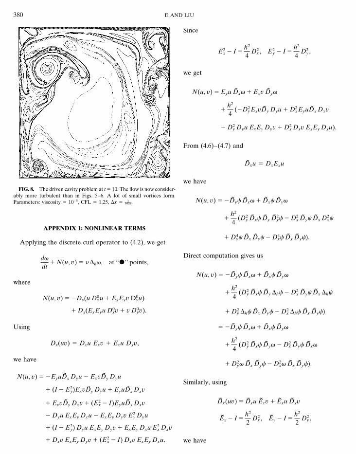
VORTICITY BOUNDARY CONDITION FOR FINITE DIFFERENCE SCHEMES 379
FIG. 7. The driven cavity problem at t 5 8. Plotted here is the vorticityFIG. 6. Same as Fig. 5, but for the stream function. At the lower rightat the lower left quadrant. The contour lines are severely stretched. Aand upper left corners, the primary vortex has induced two generations ofmushroom-like structure forms as a result of the collision of vortices.secondary vortices.Parameters: viscosity 5 1025, CFL 5 1.25, Dx 5 a;Qsf.
The calculation reported here took approximately 2tion terms are treated using centered differences. We ex-h on the C-90 machine with a single processor at theplained that while there is a severe constraint on the cellPittsburgh Supercomputing Center. A similar calculationReynolds number given by stability when first- and second-on a smaller mesh 5122 with a smaller Reynolds numberorder Runge–Kutta methods are used in time, such con-(n 5 3 3 1025) was done on a SPARC-10 work-station,traints disappear for higher order Runge–Kutta methods.and that took about three days. Obviously there is a lotThis is a significant fact with regard to the efficiency ofof room for improvement. We will return to this in acentered schemes.separate paper [4].
The third issue we discussed is the relation between theMAC scheme and the second-order centered difference
5. CONCLUSIONS schemes in the vorticity-stream function formulation, cou-pled with various local formulas for the vorticity boundarycondition. We showed that the MAC scheme is the sameLet us summarize the issues discussed in this paper.
The first issue we discussed was the local and global as the standard second-order centered difference schemein the vorticity-stream function formulation, and the localvorticity boundary conditions. We showed that Anderson’s
global vorticity boundary condition can always be realized formulas for the vorticity boundary condition can be trans-lated into local formulas for the velocity boundary condi-by local formulas, the simplest case being Fromm’s for-
mula. The non-locality of Quartapelle’s vorticity boundary tion and vice versa. In particular, Thom’s formula trans-lates to the reflection boundary condition for the MACcondition comes from the fact that the viscous term is
insisted to be treated implicitly. Therefore even the seem- scheme.From these discussions we arrive at the following basicingly local vorticity boundary condition turns out to be
global. design principles: (1) The viscous term should be treatedexplicitly for finite difference schemes in the vorticity-A majority of the discussions in the literature on global
vorticity boundary conditions resemble Quartapelle’s, so stream function formulation. If one insists on treating theviscous terms implicitly, then it is much better to use thethe global nature of the vorticity boundary condition is
really a result of the implicit treatment of the viscous projection method [3]. (2) One should use at least third-order Runge–Kutta methods in time in connection withterm.
The second issue we discussed is the cell Reynolds num- centered differences in space for high Reynolds numberflows.ber constraint in connection with the fact that the convec-
380 E AND LIU
Since
E2x 2 I 5
h2
4D2
x , E2y 2 I 5
h2
4D2
y ,
we get
N(u, v) 5 Eyu Dxg 1 Exv Dyg
1h2
4(2D2
y ExvDy Dyu 1 D2x EyuDx Dxv
2 D2y Dyu ExEy Dyv 1 D2
x Dxv ExEy Dxu).
From (4.6)–(4.7) and
Dxu 5 DxExu
we haveFIG. 8. The driven cavity problem at t 5 10. The flow is now consider-
ably more turbulent than in Figs. 5–6. A lot of small vortices form.N(u, v) 5 2Dyc Dxg 1 Dxc DygParameters: viscosity 5 1025, CFL 5 1.25, Dx 5 a;Qsf.
1h2
4(D2
y Dxc Dy D2yc 2 D2
x Dyc Dx D2xc
APPENDIX 1: NONLINEAR TERMS
1 D4yc Dx Dyc 2 D4
xc Dx Dyc).Applying the discrete curl operator to (4.2), we get
Direct computation gives usdgdt
1 N(u, v) 5 n Dhg, at ‘‘d’’ points,
N(u, v) 5 2Dyc Dxg 1 Dxc Dygwhere
1h2
4(D2
y Dxc Dy Dhc 2 D2x Dyc Dx Dhc
N(u, v) 5 2Dy(u D0x u 1 ExEyv D0
yu)
1 Dx(ExEyu D0xv 1 v D0
yv). 1 D2y Dhc Dx Dyc 2 D2
x Dhc Dx Dyc)
5 2Dyc Dxg 1 Dxc DygUsing
Dx(uv) 5 Dxu Exv 1 Exu Dxv, 1h2
4(D2
y Dxc Dyg 2 D2x Dyc Dxg
we have1 D2
yg Dx Dyc 2 D2xg Dx Dyc).
N(u, v) 5 2EyuDx Dyu 2 ExvDy DyuSimilarly, using
1 (I 2 E2y)ExvDy Dyu 1 EyuDx Dxv
Dx(uv) 5 Dxu Exv 1 Exu Dxv1 ExvDy Dxv 1 (E2x 2 I)EyuDx Dxv
2 Dyu ExEy Dxu 2 ExEy Dyv E2y Dyu Ex 2 I 5
h2
2D2
x , Ey 2 I 5h2
2D2
y ,1 (I 2 E2
y) Dyu ExEy Dyv 1 ExEy Dxu E2x Dxv
1 Dxv ExEy Dyv 1 (E2x 2 I) Dxv ExEy Dxu. we have

VORTICITY BOUNDARY CONDITION FOR FINITE DIFFERENCE SCHEMES 381
u21/2 5 2u1/2 , un11/2 5 2un21/2 .2Dx(Dyc g) 1 Dy(Dxc g)
5 2Dyc Dxg 1 Dxc Dyg 1 (I 2 Ex) Dyc Dxg Clearly,
1 (Ey 2 I) Dxc Dyg 1 (I 2 Ex)g Dx Dyc D2xui11/2 5 u0(xi11/2) 1 O(h2) for i 5 1, ..., n 2 2.
1 (Ey 2 I)g Dy DxcAt x1/2 ,
5 2Dyc Dxg 1 Dxc Dyg
D2xu1/2 5
u3/2 2 3u3/2
h2 5u(x3/2) 2 3u(x3/2)
h2 114
u0(0)1h2
2(2D2
x Dyc Dxg 1 D2y Dxc Dyg
2 D2xg Dx Dyc 1 D2
yg Dy Dxc).5
34
u0(x1/2) 1h8
u-(0) 214
u0(0) 1 O(h2)
Therefore,5 u0(x1/2) 1 O(h2).
N(u, v) 5 2Dyc Dxg Similarly, we have
1 Dxc Dyg 1 As[Dyc Dxg 2 Dx(Dyc g)]
D2xun21/2 5
u(xn23/2) 2 3u(xn23/2)h2 1
14
u0(1)2 As[Dxc Dyg 2 Dy(Dxc g)]
5 2As[Dyc Dxg 1 Dx(Dyc g)] 5 u0(xn21/2) 1 O(h2).
1 As[Dxc Dyg 1 Dy(Dxc g)].This gives
APPENDIX 2: CONSISTENCY NEAR THE BOUNDARY u(xi11/2) 2 ui11/2 5 O(h2).
FOR THE REFLECTION TECHNIQUEThe boundary condition mentioned in [14],
If we use the reflection boundary condition ui,21/2 1u21/2 5 Ad(u3/2 2 6u1/2 1 8uG),ui,1/2 5 0 in the MAC scheme, a simple truncation error
analysis at x1/2 givescorresponds to the first formula of Orszag and Israeli (seeTable I in Section 2).
D2xu(x1/2 5
34
u0(x1/2) 1h8
u-(0) 1 O(h2),
ACKNOWLEDGMENTS
suggesting that the operator D2x is not consistent with the We are very grateful to Gretar Tryggvason for his suggestions which
Laplacian near the boundary. This issue has been raised greatly improved the presentation of this paper. We also thank AlexanderChorin for very helpful discussions. The work of Weinan E was supportedin several places, including [14]. We show here that a moreby the NEC Research Institute Inc., the Sloan Foundation under Grantsophisticated error analysis reveals that the overall scheme93-6-6, a Sloan Foundation Fellowship, and NSF Grant DMS-9303779.still has second-order accuracy. We explain this by a sim-The work of J.-G. Liu was supported in part by NSF Grants DMS-9505275
ple example and DMS-9304580. The computations were done at the Pittsburgh Super-computing Center.
u0 5 f, u(0) 5 (1) 5 0REFERENCES
with the standard centered difference applied to the grid1. C. R. Anderson, J. Comput. Phys. 80, 72 (1989).points xi11/2 5 (i 1 As) Dx, i 5 0, 1, ..., n 2 1 and the2. W. R. Briley, J. Fluid Mech. 47, 713 (1971).boundary condition u21/2 1 u1/2 5 0, un11/2 1 un21/2 5 0. Let3. A. J. Chorin, Math. Comput. 22, 745 (1968).
4. W. E and J.-G. Liu, J. Comput. Phys., submitted.ui11/2 5 u(xi11/2) 2
h2
8[u0(0) 1 (u0(1) 2 u0(0))xi11/2] 5. W. E and J.-G. Liu, preprint.
6. U. Ghia, K. N. Ghia, and C. T. Shin, J. Comput. Phys. 48, 387 (1982).for i 5 0, 1, ..., n 2 1 7. P. M. Gresho, Annu. Rev. Fluid Mech. 23, 413 (1991).
8. P. M. Gresho, Adv. Appl. Mech. 28, 45 (1992).
9. F. H. Harlow and J. E. Welch, Phys. Fluids 8, 2182 (1965).and

382 E AND LIU
10. H. D. Henshaw, H.-O. Kreiss, and L. G. M. Reyna, Comput. & Fluids, 16. L. Quartapelle and F. Valz-Gris, Int. J. Numer. Methods Fluids 1,129 (1993).to appear.
11. B. C. Johansson, J. Comput. Phys. 105, 233 (1993). 17. M. Reider, Ph.D. dissertation, UCLA, 1992 (unpublished).
18. P. J. Roache, Computational Fluid Dynamics (Hermosa, Albuquer-12. S. A. Orszag and M. Israeli, Annu. Rev. Fluid Mech. 6, 281 (1974).que, NM, 1982).13. S. A. Orszag, M. Israeli, and M. O. Deville, J. Sci. Comput. 1, 75
(1986). 19. R. Schreiber and H. B. Keller, J. Comput. Phys. 49, 310(1983).14. R. Peyret and T. Taylor, Computational Methods for Fluid Flow
(Springer-Verlag, New York/Berlin, 1983). 20. A. Thom, Proc. Roy. Soc. London Sect. A 141, 651 (1933).
21. D. C. Thoman and A. A. Szewczyk, Phys. Fluids 12 (1969), II-15. L. Quartapelle, Numerical Solution of the Incompressible Navier–Stokes Equations (Birkhauser, Berlin, 1983). 76–II-87.