Volume Visualization Presented by Zhao, hai. What’ volume visualization Volume visualization is...
33
Volume Visualization Presented by Zhao, hai
-
Upload
neal-harper -
Category
Documents
-
view
233 -
download
3
Transcript of Volume Visualization Presented by Zhao, hai. What’ volume visualization Volume visualization is...

Volume Visualization
Presented by
Zhao, hai

What’ volume visualization
• Volume visualization is the creation of graphical representations of data sets that are defined on three-dimensional grids. Volume data sets are characterized by multidimensional arrays of scalar or vector data. These data are typically defined on lattice structures representing values sampled in 3-D space.
• many objects and natural phenomena are 3D volumes of data.

Contd..
• Volume visualization can be traced back to the beginning of the 1970s.
• Recently, volume visualization has matured as a primary field of computer graphics.

• Volume visualization is concerned with the representation, manipulation, and rendering of volumetric data.

Application Domains
• Spinal Cord/Neurology
• Earth and Atmospheric

• Visual human/medical images
• Molecular science

• Paleontology
• Aeronautics

• Joint simulation/ Engineering mechanical
• Oceanography

Taxonomy of Volume visualization

Volume Visualization Pipeline

Basic Concept
• A voxel is the 3D counterpart of the 2D pixel. Each voxel is a quantum unit of volume and has a numeric value associate with it that represents some measurable properties or independent variables of the real objects, i.e., color, density, time.

• volume rendering
To visualize the volume dataset, primitives can be directly projected into 2D pixel space and stored as a raster image in a frame buffer. It involves both the viewing and the shading of the volume image.
Basic Concept

• the volume data can be first converted into geometric primitives in a process called isosurfacing, isocontouring, and surface extraction.
Basic Concept

• surface rendering
the geometric primitives are rendered to the screen (I.e., conventional geometric rendering). It involves the isosurfacing, the viewing, and the shading stages
Basic Concept


• data acquisition.
The sources of volume data are sampled data of real objects. Sampled data are acquired by 2D or 3D multi-channel scanners that measure the real world object and usually produce a sequence of 2D cross sections of the object.
Enhancement
Is to change them into a form that is more informative, filtered and uniform.
Reconstruction
The missing data between slices or between scattered points are interpolated.

• Manipulation stage includes geometrics, domain transformations.
• Classification stage is either a thresholding step or a material classification step. Thresholding is used primarily in the surface-rending approach, i.e., all values below it are assigned “0”, while all those above are set to “1”.

• Mapping stage maps the 3D voxel data into geometric or display primitives.
The choice of display primitive depends on whether volume rendering or surface rendering is used.
• Volume viewing
Determines the parts of the 3D scene that are visible
• Volume shading
Shading techniques compute the intensity/color value that reaches the viewer’s eye from each point of the visible surface.
It has two goals: one is provide optimal visual recognition for discernment of the displayed objects. The other goal is show the natural appearance of real objects.

representation
• The binary-array representation
Scene is digitized that the density must be one of the integers between a lower limit L and an upper limit U. If L =0 and U =1, then we say that scene is binary scene.

• Segment Endpoint Representation
J, Sj, i1L, i1
R,i2L, i2
R, … ijL, ij
R

Directed contour representation

Display
• Ensuring only that part of the object that is visible from the given view is displayed
• Assigning a shade to the visible surface to impart a 3D illusion.

Display from the binary-array representation
• Back-to-front method
For any 3D scene, there is a 3*4 transformation matrix T
U = T11x + T12y + T13z + T14
V = T21x + T22y + T23z + T24
W = T31x + T32y + T33z + T34
Eliminationg x and y
W = a + bz

Earth models

The procedure of earth model

1. Contouring by Triangulation
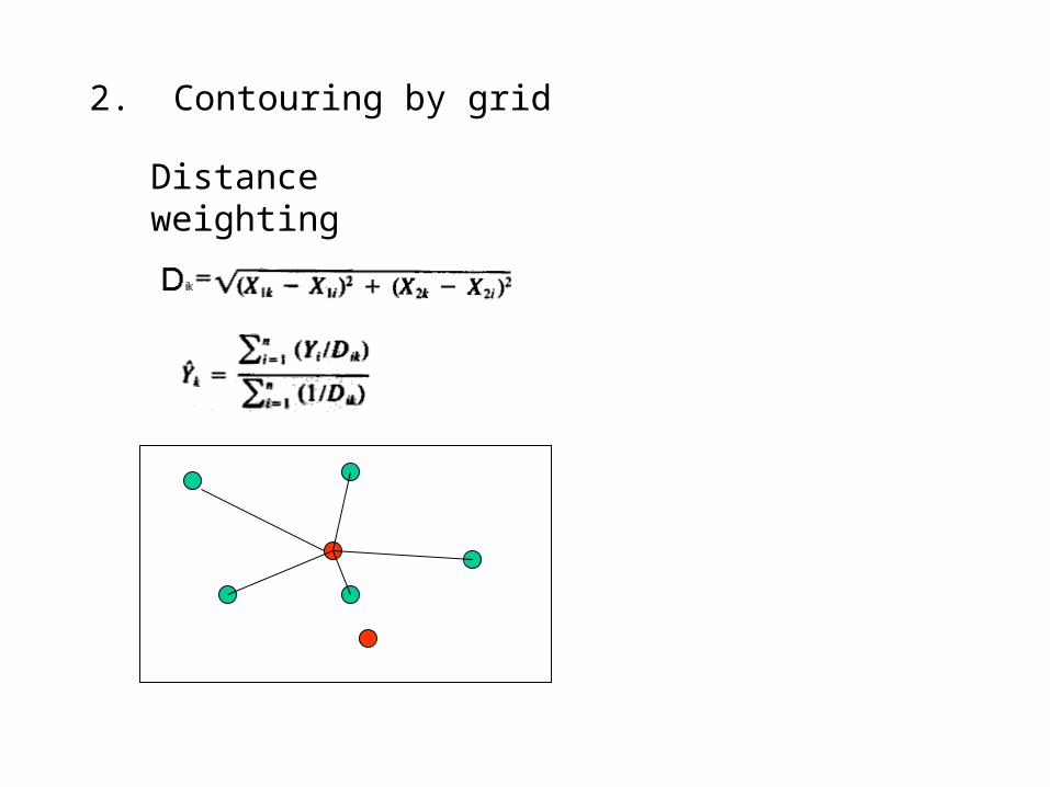
2. Contouring by grid
Distance weighting

Tread surface Models:
Y = b1X1 + b2X2 +…+b0
Where the b’s are coefficients
And X’s are some combination of the coordinates.
Kriging:
Y = Wi Yi

• Trace contour line
• Line smooth
Another algorithm
Application
• Interactive Surgical Planning
• Earthvision
• Rendering Volumetric data in molecular system
• Animated 3D CT imaging

Reference
• Volume visualizationArie kaufman
IEEE computer Society Press 1991
• Statistics and data analysis in GeologyJohn C. Davis
John Wiley and Sons, inc 1986
• www.dgi.com